Validating Commonly Used Indicators for Community Resilience Measurement
Abstract
This study quantitatively examines indicators frequently used to estimate community resilience and proposes a method for assessing the validity of indicators used in community resilience measurement. An array of 18 indicators and related measures were identified as being common to existing methodologies. A comprehensive and replicable method that can evaluate the reliability and validity of community resilience indicators was then employed to explore the appropriateness of indicator selection by comparing different sets of measures. Multiple internal consistency test methods, such as Cronbach’s alpha, correlation analysis, cluster analysis, and classification tree, were conducted to address varying aspects of community resilience and to estimate commonalities in indicator selections. Structural equation modeling (SEM) provided a system to investigate indicators’ validity and overall performance in a hypothetical construct of community resilience predicting a proxy of community resilience outcomes. In exploring internal consistency and external validation of indicators, the importance of conducting validation studies is highlighted. To ensure indicators are ready for use among practitioners and policymakers, the quality of indicators needs to be tested and clearly stated in the context of other indicators and empirical outcomes of community resilience.
Introduction
The concept of resilience has gained an incredible amount of attention over the past two decades and has been increasingly applied in fields of study focused on climate change, natural hazards, and disasters (Klein et al. 2003; Manyena 2006; Zhou et al. 2010). In particular, achieving community resilience—which this study defines as “the ability to prepare for anticipated hazards, adapt to changing conditions, and withstand and recover rapidly from disruptions” (The White House 2013)—has been a long-sought goal of governmental officials, disaster response professionals, and academic researchers. Effective implementation of policy or governance for achieving community resilience has been hindered by a variety of factors, one of which is that there is no agreed upon process for measuring progress (CARRI 2013; Ostadtaghizadeh et al. 2015; Asadzadeh et al. 2017; Patel et al. 2017; Edgemon et al. 2020). The ability to track baseline resilience of a community and the effect of any intervention is a key step for formulating options, communicating progress, and if needed, adapting policy (Linkov and Trump 2019).
The challenges in community resilience measurement arise from several factors including the disparate disciplines and fields using the concept, numerous definitions, vast number of potential indicators, and lack of agreement on how indicators should be assessed for validation testing (Linkov and Trump 2019). Overcoming difficulties in validation testing can be especially important because doing so can establish that any chosen set of indicators is predictive of resilience, thereby increasing indicator credibility—an important factor in generating usable science for planning, policy making, and other impactful decision-making purposes (Cash et al. 2003; Wilson et al. 2021). However, establishing the predictive relationship of concepts like social capital, which cannot be directly observed, to community resilience, which also cannot be directly observed, introduces considerable technical and data challenges. As a result, most community resilience indicator studies focus on a subset of steps in the validation process, such as the internal consistency of indicators, and prediction of observed variables, such as property damage. Whereas the latter can provide some information about the credibility of a set of indicators, it falls short of fully establishing their relation to community resilience, which is an emergent multidimensional concept.
Handling unobserved, or latent, variables is a common problem in other disciplines, especially in psychology, education, and health care systems analysis, where indicators also play an important role in management. This paper argues that methods commonly used in these disciplines can be a useful addition to current practice. In particular, the following presents a case study using structural equation modeling (SEM), a method that allows for measuring the relationship between unobserved variables, as measured by sets of indicators. Whereas adopting this method introduces its own technical and data challenges, this study argues it provides a comprehensive set of tools for establishing validity.
Background
Part of the challenge of indicator validation is that validation is a multipart concept and process and the relative importance of each part of the process is dependent on the specific scientific discipline or field of application. Not all community resilience indicator frameworks fully acknowledge and engage with the multidimensional nature of validation. Thus, as a starting point for background, this case study begins with scientific fields, such as psychology and program evaluation, where measurement models are more consistently developed and tested. For example, psychometrics has a long tradition of conceptualizing validation of measurement scales and models in four areas: predictive, concurrent, content, and construct validity. Predictive validity presents the ability of the model or scale to estimate scores on a criterion outcome. Similarly, concurrent validity compares the results of the model or scale with other established scales or measures that have been validated previously. Content validity relates to the ability of the measure to holistically capture the multiple aspects of the phenomenon being measured (for example, the social, economic, and built environment components of community resilience). Last, and arguably most importantly, construct validity relates to the relationships between a model and what it purports to be measuring (Cronbach 1951; Strauss and Smith 2009). Each of these types of validity, among others, has recommended best practices for testing. For example, construct validity is often assessed through a series of rigorous hypothesis tests to determine whether or not dependent variables meet a set of assumptions based on previous findings and theory. The appropriateness of the dependent variable(s) is then determined by the expected strength and direction of these relationships (Cronbach 1951; Strauss and Smith 2009). Much of the modern discourse around model validation revolves around construct validity—validation as part of an evaluation process that determines to what degree a model is adequate or fit for its purpose (Parker 2020).
Validation Approaches in Community Resilience Frameworks
Community resilience, as a concept indicating the capacity to recover and adapt in a timely manner following acute stressors, can be revealed after a disruptive event through failure (Galaitsi et al. 2021); however, its presence during nondisruptive moments is harder to recognize and therefore, to measure. This is because community resilience is a latent variable or a variable that cannot be directly observed. Bollen (2001) noted that indicators help recognize and fill the gaps between social science concepts and measures. Latent variables can represent concepts; measurement models relate latent variables to reflective indicators, and causal models represent structural effects of formative indicators on latent variables (Bollen and Bauldry 2011). When concerns have appeared in previous studies, the focus has been on either internal consistency of measurement models or external validation of causal models to assess reliability and validity of a composite indicator.
For the assessment of internal consistency of the measurement model itself, many community resilience frameworks have used similar approaches, such as correlation analysis, Cronbach’s alpha, principal component analysis, and exploratory factor analysis. However, there is less consensus in methods used to validate the causal models proposed within the indicator frameworks. For example, in a review of community resilience models (Loerzel and Dillard 2021; Walpole et al. 2021), only two community resilience frameworks have presented external validation assessments: Community Disaster Resilience Index (CDRI) (Peacock et al. 2010) and National Oceanic and Atmospheric Administration (NOAA) composite indicators of community well-being and environmental condition (Dillard et al. 2013). The multivariate regression models presented as part of the development and testing of these frameworks largely adhere to an approach where a series of hypotheses about the construct validity are tested using selected dependent variables.
Previous quantitative resilience analyses primarily focused on physical impacts of natural hazards like damage itself or the outcomes of damage as a notion of resilience—more damage equates to lower resilience and less damage to higher resilience. Several journal articles report on testing community resilience indicators using dependent variables related to disaster impacts. Multivariate regression models have been frequently used with a selection of dependent variables, such as decreased population, representing postdisaster outmigration (Myers et al. 2008), damage assessment by remote sensing (Burton 2010), Hazard US Multi-Hazard (HAZUS-MH) modeled expected earthquake damage (Schmidtlein et al. 2011), changes in mail deliveries (i.e., actively receiving residential mail) as an estimate of repopulation and recovery (Finch et al. 2010), observed property losses, fatalities, and frequency of disaster declarations (Bakkensen et al. 2017), Individual assistance program applicants, affected renters, flood-damaged applicants, property losses, and water depths (Rufat et al. 2019), and postdisaster emergency, food, and shelter needs (Crowley 2021). The primary difference between these analyses and the comprehensive validity assessment approach proposed here is one of scope. The population of emphasis for the proposed method for validity testing encompasses all counties in the United States and is intended for relevance to all disasters and to counties (and time periods) with no disasters. The case-study-oriented approaches, such as cross-sectional study designs with dependent variables and indicators relying on a specific disaster event in a designated study area, are not independently adequate, though they are instructive. In addition to using multivariate regression models, another approach to validation assessments is to compare findings from frameworks and consensus indicators, which can contribute to establishing content validity. Cutter et al. (2014), Bakkensen et al. (2017), and Cutter and Derakhshan (2019) have compared outcomes of several consensus indicators, such as baseline resilience index for communities (BRIC), CDRI, social vulnerability index (SoVI) (Cutter et al. 2003; HVRI 2014), resilience capacity index (RCI) (Foster 2012), and social vulnerability index (SVI) (Flanagan et al. 2011). Bakkensen et al. (2017) highlighted the gaps between frameworks’ objectives, selected indicators, and community resilience outcomes; not all frameworks were statistically significant across dependent variables (e.g., property damage, fatalities, and disaster declarations), and some of them performed the opposite of what was expected. In conjunction with the lack of consensus in selections of dependent variables and indicators, the mismatches between estimated indices and dependent variables raise questions about the validity of existing community resilience frameworks.
Selection of Indicators for Validation Study
Among the challenges of community resilience measurement is the vast number of potential indicators. To develop and apply a method for validation testing, this study relied on foundational work conducted by NIST researchers to identify a suite of commonly used indicators along with sets of practically obtained measures. Whereas the process for identifying the commonly used indicators was systematic, there is no proposition that this suite forms an ideal framework for community resilience. Instead, the commonly used indicators are ripe for testing and serve as the ideal proving grounds for the validation methods proposed here.
NIST researchers have been examining community resilience frameworks and methodologies since 2015. This work began with a small review of nine frameworks (Lavelle et al. 2015) and has since expanded to include a compilation of nearly 4,000 indicators across 56 frameworks and the development of methods for comparing dissimilar framework components (Loerzel and Dillard 2021; Walpole et al. 2021). The intent was to develop a set of commonly used indicators that should be further evaluated for theoretical evidence of the linkage of these indicators to the concept of community resilience and for statistical evidence of a relationship to community resilience that fits expectations. The analysis began by narrowing the scope from a search for consensus among the nearly 4,000 indicators to a search among 330 indicators in seven frameworks. After developing and applying a coding scheme using system types and system attributes, the study identified 18 indicators that could be internally and externally justified as common through the coding of the frameworks and a comparison with seven reviews of resilience. Table 1 lists these 18 indicators, the related measures, and data source. Seven additional measures were selected to assess the consistency of commonly used indicators with a subset of less common indicators in the community resilience frameworks, such as race, female life expectancy, children in poverty, Supplemental Nutrition Assistance Program (SNAP) participants, and housing unit statistics: value, mobile home type, and vacancy.
| Indicator | Measure | Source |
|---|---|---|
| Voting | • Turnout of registered voters | Leip (2016) |
| • Registered voters | ||
| Educational attainment | • No high school diploma/GED | US Census Bureau (2016) |
| • GED or higher | ||
| • Bachelor’s degree or higher | ||
| • Ratio of GED to bachelor’s degree or higher | ||
| Health system labor force | • Employment: health care and social assistance sector | US Bureau of Labor Statistics (2016) |
| Civic organizations | • Arts and humanities organizations | NCCS (2016) |
| • Human services organizations | ||
| • Religious organizations | ||
| Regional economic vulnerability | • Employment: service sectors | US Bureau of Labor Statistics (2016) |
| Housing tenure | • Households: owner occupied | US Census Bureau (2016) |
| Healthcare infrastructure | • Establishments: sector 622 (hospitals) | US Bureau of Labor Statistics (2016) |
| • Number of hospital beds | CMS (2016) | |
| Housing cost | • Households: median monthly costs of housing | US Census Bureau (2016) |
| • Households: median rent | ||
| Age-based susceptibility | • Population: under 18 | US Census Bureau (2016) |
| • Population: 65 years and older | ||
| Vehicle access | • Households: no vehicle available | US Census Bureau (2016) |
| Unemployment | • Civilian labor force unemployment rate | US Census Bureau (2016) |
| Labor force participation | • Population: in labor force | US Census Bureau (2016) |
| Poverty | • Population: individuals in poverty | US Census Bureau (2016) |
| • Households: poverty | ||
| Income | • Median household income | US Census Bureau (2016) |
| • Per capita income | ||
| Inequality | • Gini index | US Census Bureau (2016) |
| • Households: income more than $200k | ||
| Telephone service | • Households: without telephone service | US Census Bureau (2016) |
| Flood exposure | • Expected annual loss | Zuzak et al. (2021) |
| • Number of events | NOAA (2021) | |
| • Property damage per capita | Center for Emergency Management and Homeland Security (2018) | |
| Health insurance | • Population: no health insurance | US Census Bureau (2016) |
| Test measures | • Race: White | US Census Bureau (2016) |
| • Female life expectancy | ||
| • Population: under 18 in poverty | ||
| • Households: participating in SNAP | ||
| • Housing units: median value | ||
| • Housing units: mobile home | ||
| • Housing units: vacant |
Various measures were used to operationalize these indicators, depending on the framework, definitions applied, and approach to measurement. The same indicator was often quantified by multiple measures across frameworks. For example, the indicator healthcare infrastructure was captured by measures including number of hospital beds, number of physicians, number of healthcare establishments, and number of hospital establishments. Instead of testing composite indices of existing frameworks, this study focused on measures as the baseline elements for developing the criteria for the consistency and validity of community resilience measurement. These common indicators and alternative operationalizations using various measures are the basis of the validation testing approach developed and applied in this paper.
To investigate the validity of the 18 indicators and various sets of measures, the NIST Tracking Community Resilience (TraCR) database served as a toolbox for the data needed. TraCR was developed to support the testing and refinement of analytical methods and for evaluating community resilience indicators. It presently contains more than 100 county-level variables representing social, economic, and physical systems, spans the years of 2000–2016, and includes more than 25 unique sources. The data cover 3,230 US counties in all 50 states. TraCR is continually updated to reflect new data, geographies, and time points; this database will ultimately be made available to the public and will contain tools for indicator calculation, and data visualization (NIST 2022).
Previous community resilience frameworks and related studies have used counties or census tracts as a contextual unit to represent a community. Counties allow for better statistical comparisons, especially for indicators conceptually rooted in larger geographic areas, such as regional economic vulnerability, and healthcare infrastructure. Mean values of measures with multiple years of data were used to mitigate annual fluctuations instead of selecting a specific year of the data. To control for varying county sizes, proportional measures were calculated based on county population or number of households followed by standardization using a z-score.
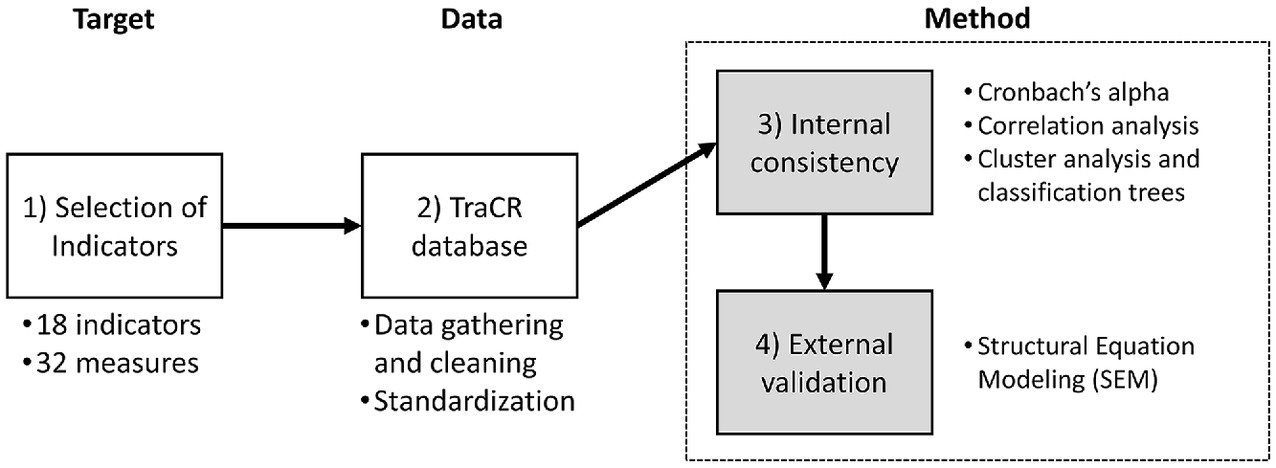
Methods
This study offers an example of a comprehensive internal consistency and external validation assessment method that can be applied to the entire United States for designing community resilience frameworks and consensus indicators at the county level. Fig. 1 shows the overarching research process after: (1) selection of commonly used indicators, and (2) development of dataset(s) in the TraCR database. These two steps are illustrated in the selection of indicators for validation study section. This study focuses on (3) internal consistency, and (4) external validation of commonly used community resilience indicators and the measures used to operationalize such indicators.
Previous frameworks have suggested theoretical backgrounds for selecting indicators and identifying commonalities across indicators. Then, a handful of dependent variables were tested in journal articles related to disaster impacts. The consistency between indicators and the overarching empirical aspects of community resilience regarding indicators and dependent variables remains in question. The main contributions of this study are comparing several internal consistency test methods used in previous frameworks, proposing an indicator validation method to overcome the research gaps in the literature, and finally, identifying indicators with remaining consistency and validation issues.
Internal Consistency Assessments
The first phase of this study is internal consistency assessments to explore the reliability of indicator selections. The motivating questions are: (1) does internal consistency exist within the indicators chosen for this study, (2) does the selection of indicators change estimates of county characteristics, and if so, and (3) which indicator drives the estimates? Importantly, this study explores consistency of both indicators and measures, which is an extra step that is needed when more than one measure can be used for an indicator. Whereas prior works acknowledge this issue, it is rarely operationalized in the internal consistency phase. The extra analysis is needed because if measures for the same indicator are in fact measuring different constructs, then each measure could result in inconsistent or unreliable estimation of shared community characteristics.
To solve these questions, this study conducts several test methods that complement each other: (1) Cronbach’s alpha analysis to check the overall consistency of all 18 indicators and consistency within each indicator for indicators with multiple measures, (2) correlation analysis to compare relationships between each pair of measures, (3) cluster analysis to identify expected differences between the estimations of community resilience, and (4) a classification tree to indicate the key drivers of cluster outcomes.
Cronbach’s alpha (Cronbach 1951) and correlation analysis are conventional testing methods of internal consistency (Peacock et al. 2010). The acceptable alpha values showing internal consistency range from 0.70 to more than 0.95 (Tavakol and Dennick 2011). However, offering an alpha is not sufficient to qualify the internal consistency of measures because a high alpha can also be achieved simply by increasing the number of items (Acock 2013). To mitigate this issue, correlation coefficients were used to compare the level of internal consistency for each measure. Instead of presenting a correlation table showing pairs of relationships, this study listed the number of correlation coefficients with an absolute value higher than 0.3 (weak relationship and higher) for each measure as a way to summarize their internal consistency regardless of the signs of the coefficients. Both analyses were based on 3,009 counties in the conterminous United States due to missing observations and listwise deletion (a 93.1% coverage based on the total of 3,230 counties).
The next question is whether the selection of measures causes inconsistency in community resilience estimates. Cluster outcomes are compared with identify patterns of community resilience characterization with different arrays of measures. If cluster outcomes are sensitive to measure choices, then theoretical validation efforts on indicator selections may not be enough to guarantee coherent estimations of community resilience. Table 2 lists the selected arrays of measures for three sets. These sets represent a hypothesized selection of measures when estimating community resilience. Sets 1 and 2 consist of one measure for each indicator. Specifically, set 1 contains measures with the highest internal consistency based on the correlation coefficients. Similarly, set 2 contains measures with the second-highest internal consistency. Set 3 contains seven test measures (under the indicator Test measures in Table 1) in addition to eight commonly used measures that are used for both sets 1 and 2 (highlighted text in bold). In this way, the estimated cluster outcomes represent the results by the measures within the structure of 18 commonly used indicators (sets 1 and 2), and by the not commonly used measures (set 3). Due to the missing observations in each indicator, 3,049, 3,016, and 3,103 counties in the conterminous United States were included in sets 1, 2, and 3, respectively (94.4%, 93.4%, and 96.1% coverages based on the total of 3,230 counties).
| Indicator | Set 1 measure | Set 2 measure | Set 3 measure |
|---|---|---|---|
| Voting | Turnout of registered voters | Registered voters | — |
| Educational attainment | No high school diploma | Bachelor’s degree or higher | — |
| Health system labor force | Employment: health care and social assistance | ||
| Civic organizations | Human services org. | Arts and humanities org. | — |
| Regional economic vulnerability | Employment: service sectors | ||
| Housing tenure | Owner occupied | ||
| Healthcare infrastructure | Est.: sector 622 (hospitals) | Number of hospital beds | — |
| Housing cost | Median rent | Median monthly costs of housing | — |
| Age-based susceptibility | Pop.: 65 years and older | Pop.: under 18 | — |
| Vehicle access | Households: no vehicle available | ||
| Unemployment | Civilian labor force unemployment rate | ||
| Labor force participation | Population: in labor force | ||
| Poverty | Housing: poverty | Pop.: individuals in poverty | — |
| Income | Med. household income | Per capita income | — |
| Inequality | Hh.: income more than $200k | Gini index | — |
| Telephone service | Households: without telephone service | ||
| Flood exposure | Property damage per capita | Expected annual loss | — |
| Health insurance | Population: no health insurance | ||
| Test measures (for set 3) | — | — | Race: White |
| Female life expectancy | |||
| Pop.: under 18 in poverty | |||
| Hh.: participating in SNAP | |||
| Housing units: median value | |||
| Housing units: mobile home | |||
| Housing units: vacant | |||
Note: Highlighted measures in bold indicate the measures that are used for all three sets; Est.: establishments; Med.: median; Org.: organizations; Pop.: population; and Hh.: households.
A two-stage clustering procedure is conducted: first, Ward’s hierarchical method to find group centroids (Ward 1963), and second, using these centroids as the initial seed points, a k-means cluster analysis (Lloyd 1982) estimates the formation of the clusters. The cluster outcomes can represent several county groups of similar characteristics by minimizing the distances from the nearest cluster center. This procedure is advocated in many studies because it tends to produce clusters with roughly the same number of observations with improved globally optimal formations (Rovan and Sambt 2003). For each cluster analysis, four groups of clusters were estimated because the scree plots of the within sum of squares (WSS) and proportional reduction of error (PRE) coefficients indicated four to six groups, and cluster outcomes with five or more groups generated underused groups.
A classification tree is a tree-structured predictive model of binary decisions (Breiman et al. 1984). Classification tree analysis identifies measures that are most strongly associated with the outcome groups by minimizing the variability within each group. The classification tree algorithm is applied to the cluster outcomes to identify key measures dividing cluster groups by utilizing the Stata and R modules (Gareth et al. 2013; Cerulli 2019). Three classification trees were derived by each set of indicators based on the optimal pruning method after testing specified sizes and mean square errors. The measures selected for the first and second nodes play a decisive role in dividing the cluster groups. For the external validation assessment, the selected measures in sets 1 and 2 were employed to generate the latent community resilience variable grounded in the perspective of commonly used indicators.
External Validation Using Structural Equation Modeling
The second phase of this study is external validation. Validity assessments need to be tested by examining how well the indicators and measures estimate observed community resilience outcomes as dependent variables. Structural equation modeling (SEM) can combine indicators and measures as a hypothetical construct—a latent variable—and test causal assumptions and interrelationships through a system of equations (Ullman and Bentler 2012).
The overarching goal of this study is to develop a simplified example of a validation assessment method with respect to commonly used indicators in the form of multiple observed covariations. Commonly used indicators and measures can be both a cause and effect of community resilience. However, for an SEM solution, including complex interrelationships between the indicators and the dependent variables will dilute the validation analysis. Furthermore, whereas a crucial aspect of resilience is the ability of systems to mitigate and recover from impacts of stressors, there is a lack of empirical evidence and systematic measures suggesting causal mechanisms between indicators and longitudinal behaviors associated with community resilience. Therefore, this study employs a straightforward modeling design with: (1) one latent variable representing an estimated community resilience by a construct of commonly used indicators, and (2) another latent variable representing an outcome of community resilience by a construct of proxy dependent variables. This analysis is aimed at assessing construct and predictive validity for test sets of community resilience indicators and measures. Construct validity is assessed by examining whether and how each indicator is related to the latent variable. Predictive validity is assessed by the equation-level goodness-of-fit measure, r-squared, to illustrate how much variance this model can explain between two latent variables. Fig. 3 in the results section shows the structure of these latent variables and related measurements.
The SEM utilizes the indicators highlighted by the classification tree analysis to construct a latent independent variable. Seven indicators were included in the classification trees by sets 1 and 2 (poverty, income, regional economic vulnerability, housing cost, education, inequality, and age-based susceptibility); therefore, corresponding seven measures were selected for the latent variable (a), estimated community resilience (household poverty, median household income, service sector employment, median rent, no high school diploma/GED, Gini index, and population 65 years and older). The number of observations is 3,107 counties in the conterminous United States (a 96.2% coverage based on the total of 3,230 counties).
On the other side, a set of proxy dependent variables can serve as the latent variable (b), outcomes of community resilience. Previous validation studies have utilized a multivariate research design estimating a single disaster-oriented dependent variable at a time by employing several measures of community resilience that are related to acute stressors following disaster events [e.g., property damage (Burton 2010), estimated losses (Schmidtlein et al. 2011), disaster-related death rates (Peacock et al. 2010), and food and shelter needs (Crowley 2021)]. In these previous studies, the community resilience dependent variables were primarily focusing on the robustness aspects of community resilience for disaster-impacted communities after major disaster events. Accordingly, these dependent variables were more suitable for a relatively small geographic area, an adjacent group of communities sharing local contexts with comparable levels and types of disaster records.
This study aims to develop validated indicators and measures to account for community-scale resilience outcomes that can include impacts of both acute and chronic stressors over time. Using a disaster-oriented dependent variable for a national-level study can mislead the estimation of community resilience due to the geographically unbalanced frequency and intensity of major disaster events. For example, the flood exposure measures have skewed distributions due to the many counties with zero or very low aggregated values from 2000 to 2016.
The assessment methodology is intended to be applicable to communities during blue skies and after hazard events. Several proxy measures can be considered as an example of comprehensive dependent variables. Variables related to overall county characteristics, such as disease related morbidity (Dillard et al. 2013), life expectancy (Gall 2007), and changes in population and occupancy (Myers et al. 2008; Finch et al. 2010), offer an extended view of community resilience that can address both acute and chronic stressors within each county’s longitudinal trend. These types of variables are suited for illustrating levels of community resilience regardless of the types and intensities of previous or expected disaster events or even without considering disaster events.
This study focuses on the population and life expectancy as quantity and quality measures of community resilience outcomes. The first proxy measure is population change. Many cities in the United States have faced urban depopulation since the 1950s as a consequence of deindustrialization and subsequent job loss and outmigration (Hollander et al. 2009). In general, for a local municipality, loss of population has been reported as a signal or a causal factor of an undergoing structural crisis rooted in economic transformations (Wiechmann and Pallagst 2012). Myers et al. (2008) and Finch et al. (2010) have utilized changes in population and housing vacancy/occupancy as an outcome of social vulnerability after disaster events. Regarding the resource allocation or prioritization for community planning and development, population is also a criterion for distributing federal and state-level entitlement programs competitively. For example, Community Development Block Grant (CDBG) uses two formulas, including the population and population growth rate variables for funding allocations (Jaroscak 2021), and the distribution of Surface Transportation Block Grant Program (STBG) is based on the relative share of local municipalities’ population (Kalla 2022).
The second and third proxy measures are female life expectancy (FLE) and change in FLE. Before the 1950s, reductions in the death rate at young ages prompted the rise in life expectancy. On the other hand, after the 1950s, most of the gain in life expectancy was due to improvements in mortality after age 65 (Oeppen and Vaupel 2002). The gain is related to advances in many interrelated social systems, such as income, education, crime, diet and nutrition, access to health care, hygiene, and medicine (Oeppen and Vaupel 2002; Riley 2001). Accordingly, life expectancy can offer information about the well-being of a county in the United States (Kulkarni et al. 2011; Correia et al. 2013; Dwyer-Lindgren et al. 2017), describing the geographic variation of health outcomes related to overall socioeconomic and race-ethnicity characteristics. In the fields of health science and sociology, life expectancy has served as one of the fundamental topics of interest for understanding biological and especially, social determinants, which are principal sources shaping the diverging health needs rooted in social inequality (Gutin and Hummer 2021). In terms of community resilience, Gall (2007) tested female and male life expectancies that account for health and quality of life to assess social vulnerability indices.
The latent dependent variable (b) consists of percent changes in population, female life expectancy, and percent changes in female life expectancy from 2000 to 2016 (US Census Bureau 2016). In this period, population growth amounts to 6.3% per county on average. The average female life expectancy is 79.7 years, and it has increased by 1.4% in the same period.
Using the SEM, a more comprehensive assessment of indicators can be conducted. Unlike multivariate regression models in the previous literature, the SEM allows for testing hypothesized patterns between latent variables, offering an option to control multicollinearity, and addressing differential importance on the aspects of the indicators and dependent variables. In addition, the latent structures mitigate the imperfect nature of each measure by taking into account measurement errors. The SEM utilized an intercept-suppressed option for each measure to reflect the zero mean values of the z-score standardized variables.
Results
Internal Consistency of Indicators and Measures
Internal consistency reflects the reliability of indicators and measures. In Table 3, Cronbach’s alpha coefficient () illustrates the internal consistency of indicators with two or more measures. The alpha coefficient for all measures () suggests a relatively high degree of internal consistency, taken as a whole. However, for the internal consistency of each indicator, the result shows the relative low alphas for voting (), inequality (), and flood exposure (). Low alpha values imply that the measures within these indicators capture different dimensions of their indicator, may not consistently provide compatible outcomes, and may not be used interchangeably.
| Indicator | Measure | Cronbach’s alpha coefficient | No. of correlation coefficient (absolute value ) |
|---|---|---|---|
| Total | All measures | 0.88 | — |
| Voting | • Turnout of registered voters | 0.33 | • 18 |
| • Registered voters | |||
| • 0 | |||
| Educational attainment | • No high school diploma/GED | 0.84 | • 26 |
| • GED or higher | • 23 | ||
| • Bachelor’s degree or higher | • 24 | ||
| • Ratio of GED to bachelor’s degree | • 22 | ||
| Health system labor force | • Employ.: health care and social assist. | — | • 5 |
| Civic organizations | • Arts and humanities organizations | 0.78 | • 11 |
| • Human services organizations | • 16 | ||
| • Religious organizations | • 7 | ||
| Regional economic vulnerability | • Employment: service sectors | — | • 11 |
| Housing tenure | • Owner occupied | — | • 10 |
| Healthcare infrastructure | • Establishments: sector 622 (hospitals) | 0.69 | • 6 |
| • Number of hospital beds | • 3 | ||
| Housing cost | • Median monthly costs of housing | 0.82 | • 19 |
| • Median rent | • 20 | ||
| Age-based susceptibility | • Population: under 18 | 0.63 | • 6 |
| • Population: 65 years and older | • 14 | ||
| Vehicle access | • Households: no vehicle available | — | • 13 |
| Unemployment | • Civilian labor force unemployment rate | — | • 18 |
| Labor force participation | • Population: in labor force | — | • 22 |
| Poverty | • Population: individuals in poverty | 0.94 | • 25 |
| • Households: poverty | • 26 | ||
| Income | • Median household income | 0.94 | • 24 |
| • Per capita income | • 22 | ||
| Inequality | • Gini index | 0.19 | • 14 |
| • 19 | |||
| • Households: income more than $200k | |||
| Telephone service | • Households: without telephone service | — | • 15 |
| Flood exposure | • Expected annual loss | 0.35 | • 1 |
| • Number of events | • 0 | ||
| • Property damage per capita | • 1 | ||
| Health insurance | • Population: no health insurance | — | • 19 |
| Test measures | • Race: White | 0.79 | • 16 |
| • Female life expectancy | • 26 | ||
| • Population: under 18 in poverty | • 26 | ||
| • Households: participating in SNAP | • 26 | ||
| • Housing units: median value | • 18 | ||
| • Housing units: mobile home | • 23 | ||
| • Housing units: vacant | • 7 |
Note: Highlighted values in bold indicate relative higher levels of inconsistency: less than 0.7 for Cronbach’s alpha and less than or equal to 5 for the number of correlation coefficients.
For each indicator, a relative comparison of measures is conducted through correlation analysis, shown in Table 3. The number of correlation coefficients (how many coefficients having an absolute value greater than 0.3) illustrates the overall consistency for each measure, presenting the number of at least weak or higher relationships with the other measures. There are 39 measures, and a measure has a total of 38 pairs of correlation coefficients. For example, the turnout of registered voters measure has 18 correlation coefficients higher than an absolute value of 0.3. In Table 3, highlighted values in bold indicate relative higher levels of inconsistency: less than 0.7 for Cronbach’s alpha and less than or equal to 5 for the number of correlation coefficients. These cutoff values are a conservative approach compared with the previous studies (Tavakol and Dennick 2011) and a convenient cutoff value for highlighting 20% of the measures with potential issues.
Several examples are provided to show internal consistency issues. The first example is the voting indicator. Whereas the turnout of registered voters measure has 18 weak or higher correlation coefficients, the measure of registered voters appears not to be internally consistent. In addition, the drastic difference between the numbers of correlation coefficients implies that these measures may not operationalize the shared aspects of the indicator.
In contrast to the voting indicator, both measures in the inequality indicator (Gini index and households with income more than $200k) are reasonably correlated to the other measures (14 and 19 weak or higher relationships, respectively). However, the low alpha coefficient for the inequality indicator () suggests that they are not measuring the same indicator concept; both measures may represent different dimensions of inequality because the household income more than $200k measure only reflects the upper side of the inequality distribution.
The measures representing flood exposure encompass inconsistency issues rooted in the multiple dimensions within the indicator. The low alpha coefficient value () and number of correlation coefficients for each measure (one, zero, and one) imply that the measures of expected losses, number of events, and damage assessments are not consistent within the flood exposure indicator and with the other measures. Similarly, measures related to the health system labor force and healthcare infrastructure indicators show potential issues regarding the number of correlation coefficients.
A cluster analysis was performed on the three sets of measures shown in Table 2. The cluster outcomes assigned counties with similar characteristics to four groups using the 18 commonly used indicators as a baseline structure (the set 1 and set 2 measures) and using seven test measures and eight commonly used measures (the set 3 measures). Cronbach’s alpha results are more than the 0.70 minimum value standard for the three sets of measures (0.80, 0.78, and 0.82, respectively).
Fig. 2 shows the cluster outcomes for the three sets of measures with the county boundaries and OpenStreetMap background (US Census Bureau 2010; OpenStreetMap Contributors 2022) made with QGIS (QGIS Development Team 2022). The first three maps—Sets 1, 2 and 3—indicate that the selection of measures can alter assessed commonalities among the counties. The last map—Differences—compares the three cluster outcomes. The cluster outcomes are relatively stable when selecting similar measures within the structure of commonly used indicators. Between the cluster outcomes generated by the set 1 and set 2 measures, the overall geographical patterns resemble each other; 83% of the counties have the same cluster outcomes (36% in turquoise and 47% in light gray counties in the Differences map).
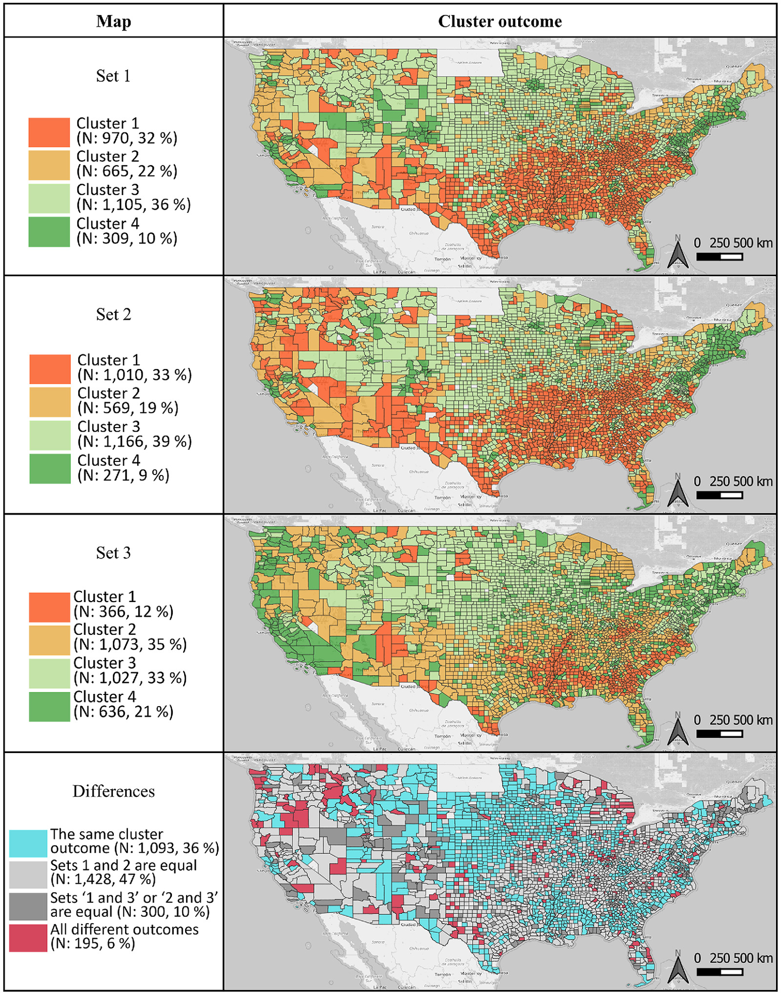
In contrast, the cluster solutions based on the set 3 measures yielded a dissimilar result; only one out of two counties maintained their cluster outcomes compared with the set 1 and set 2. Consequently, only 36% of the counties have equal cluster outcomes for all three sets. This points to a potential limitation for using different arrays of indicators and measures to evaluate community resilience. A framework with a subset of indicators and measures may risk having inconsistent or unstable community resilience estimations, depending on the selection of measures. Given that indicators are often proposed without measures specified, the differences between the three sets of measures represent a challenge in community resilience measurement.
Fig. 5 in the appendix, the classification tree diagrams illustrate the core structure of the selected measurement sets that inform the cluster outcomes. Whereas the cluster outcomes show uncertain patterns, especially for the set 3 measures, the classification tree analyses indicate relatively coherent results in understanding the major drivers of commonalities for the indicators in the three sets. All the classification trees highlight the poverty indicator, or measures of poverty, as the key determining factor. The lengths of the branches attached to the first nodes indicate that these first nodes accounted for a considerable amount of variations. Both set 1 and set 2 classification trees selected the households in poverty and individuals in poverty measures for their first nodes. For set 3, the Supplemental Nutrition Assistance Program (SNAP) participants measure stands out; it is interpreted as a combined measure of poverty and income. The indicators identified as the first and second nodes in set 1 and 2 (i.e., poverty, income, regional economic vulnerability, housing cost, education, inequality, and age-based susceptibility) are selected to form the latent variable (a) in the SEM.
External Validation of Community Resilience
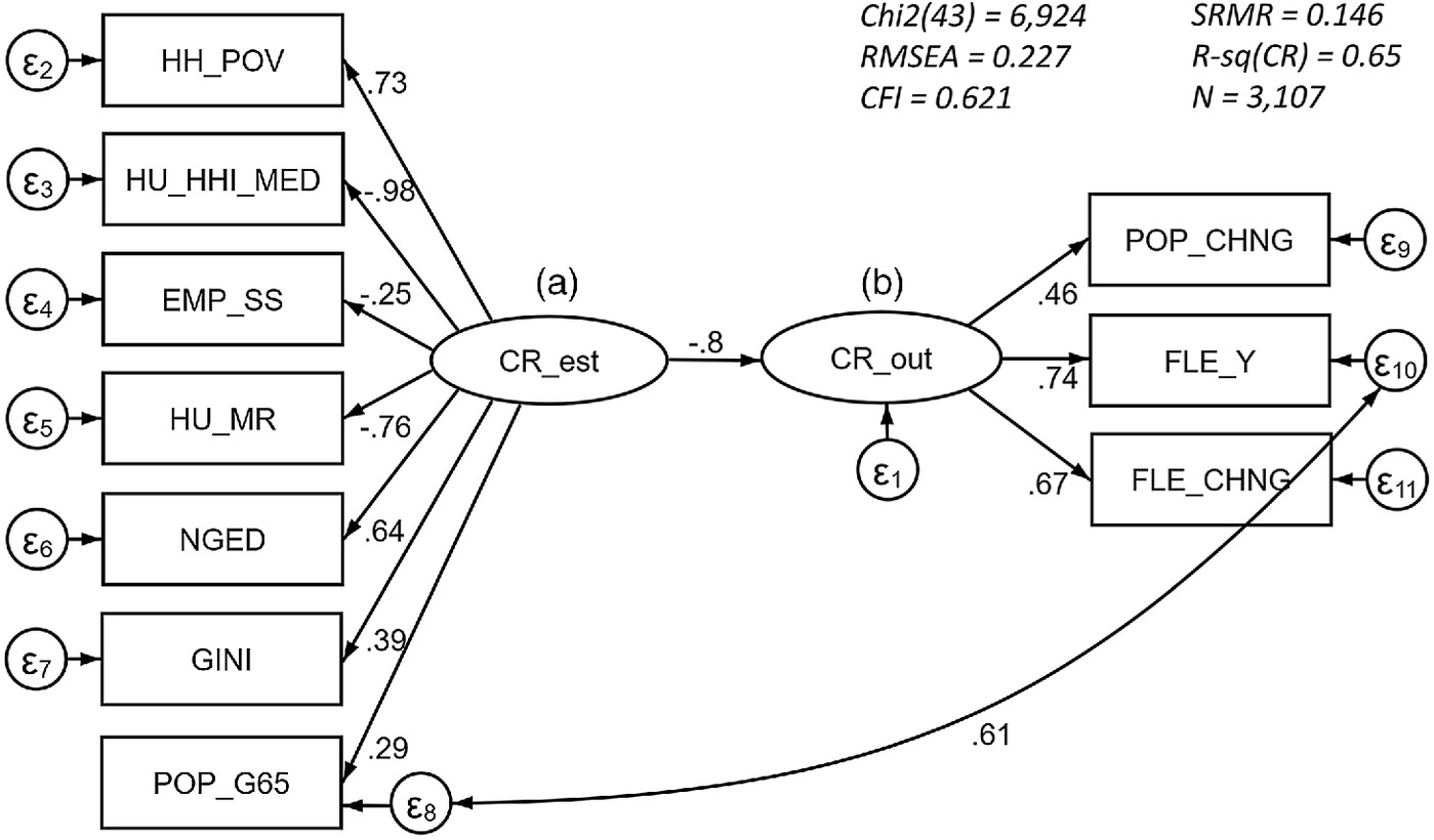
Fig. 3 graphically illustrates the structure of SEM with two latent variables. The latent variable “CR_est” (stands for estimated community resilience) is intended to reflect one dimension of community resilience (with an assumption that other dimensions exist and are not represented in this model), and the latent variable “CR_out” (stands for community resilience outcomes) reflects the construct of community resilience outcomes. Between the latent variables, the model used a correlated error term connecting the population more than 65 and female life expectancy because both items are rooted in the same aspect of mortality. The SEM result is displayed with the standardized coefficients (all variables were adjusted to have a variance of 1.0) and the goodness of fit statistics. Table 4 shows unstandardized coefficients (factor loadings with the fixed loading of the first variable at 1.0) indicating the form of the relationship and standardized coefficients () indicating the strength of an association (Acock 2013).
| Variable | Label | Unstandardized coefficient | Standardized coefficient () |
|---|---|---|---|
| Structural | |||
| CR_est (latent independent variable) to CR_out (latent dependent variable) | |||
| Measurement: CR_est | Latent independent variable | ||
| Poverty—households: poverty | 1 | 0.73 | |
| Income—median household income | |||
| Regional economic vulnerability—employment: service sectors | |||
| Housing cost—median rent | |||
| Educational attainment—no high school diploma | 0.88 | 0.64 | |
| Inequality—Gini index | 0.53 | 0.39 | |
| Age-based susceptibility—population: 65 years and older | 0.40 | 0.29 | |
| Measurement: CR_out | Latent dependent variable | ||
| % population change | 1 | 0.46 | |
| Female life expectancy | 1.63 | 0.74 | |
| % FLE change | 1.46 | 0.67 | |
| Covariance | POP_G65 and FLE_year | 0.40 | 0.61 |
Note: Highlighted categories in bold indicate the structural components of the model. All unstandardized and standardized coefficients are statistically significant with .
Overall, the fit statistics are less than ideal, falling short of the goodness of fit criteria (Peugh and Feldon 2020). For example, the comparative fit index (CFI) is lower than the acceptable value of 0.90 or 0.95, indicating that the model does 62.1% better than a baseline model, assuming no relationship among the variables. Although the model fit is not within the acceptable range, all variables, variances, and covariance are significant at the level.
Regarding the construct validity, most coefficients show anticipated connections with the latent variables, except the service sector employment measure (i.e., the regional economic vulnerability indicator) and the median rent measure (i.e., the housing cost indicator). The negative aspects of community resilience, such as poverty, no high school diploma, Gini index, and population more than 65, are positively related to the latent variable. The regional economic vulnerability and housing cost indicators should be related to these negative aspects. However, both indicators move together with the income indicator, which can be interpreted as a positive aspect of community resilience. In addition, the standardized coefficients () of the service sector employment, Gini index, and population more than 65 indicate relatively lower associations with the estimated community resilience.
The SEM equations are used to determine whether the selected measures provide a good estimate of community resilience. Within the CR_est latent variable, the income (), housing cost (), and poverty () indicators are strongly associated with the other indicators. The other latent variable, CR_out, shows that the cumulative proxy of community resilience is positively and significantly associated with all three dependent variables: Population change (), female life expectancy (), and female life expectancy change (). The relationship between two latent variables indicates that CR_est has a strong and significant relationship with CR_out: , , and . The r-squared value suggests that CR_est explains 65% of the variance of CR_out.
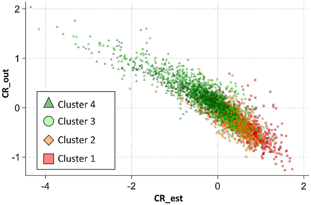
Fig. 4 illustrates the predicted factor scores of the latent variables for the cluster groups of the set 1 measures. The scatter plot shows how the indicators predict community resilience. As seen in the model, there is a negative relationship between CR_est and CR_out. Counties in cluster 1 and cluster 4 fall into two distinct groups, potentially representing low- and high-resilience counties determined by the latent variables. These two groups show a possibility of identifying high and low levels of community resilience by county clusters with a relatively smaller set of measures. On the other hand, counties in cluster 2 and cluster 3 are mixed and form a midrange community resilience group. The distribution of counties indicates a longer tail on the side of counties with higher CR_out factor scores and lower CR_est factor scores (i.e., cluster 4 counties or high-resilience counties have considerably more variance than the other county clusters).
Discussion
Given that the community resilience frameworks reviewed encompass both measurement models and causal models, they require specifying indicators’ purpose and having assessment criteria to gauge adequacy or fitness for internal consistency and external validity. Most resilience indicator frameworks are used in one of two ways. The first is to quantify resilience levels across communities for the purpose of identifying best practices in resilient communities and identifying communities that might need interventions. The second is to establish baseline resilience in a single community and track progress over time.
For either use, internal consistency is not enough to determine whether the indicators are adequate or fit for their purpose. Whereas establishing that a set of indicators reliably measures specific factors (latent variables) helps the interpretability of the resilience framework, it does not establish that it credibly predicts an aspect of resilience. This requires establishing how resilience concepts are represented by a latent variable. An approach to external validation of a resilience framework could consist of establishing outcomes, such as property losses, population decline, or a widespread decline in social capital, that are relevant for resilience as a latent variable, and establishing acceptable prediction errors for validation. If the indicator set meets the prediction error criteria for the specified outcomes, then the framework would be considered to meet the conditions for external validity.
In the external validation testing, three proxy dependent variables were proposed based on population and life expectancy. However, there is no agreement regarding dependent variables that best constitute an empirical proxy of community resilience outcomes. Previous multivariate modeling efforts relied on a single dependent variable at a time, and therefore, these models were not designed to estimate varying dimensions of community resilience outcomes as a whole. The SEM-based assessment approach suggests a baseline example of selecting and validating indicators that provide a comprehensive benchmark of community resilience. Such a benchmark could inform researchers and practitioners about how well the community resilience indicators perform for selected outcomes of community resilience.
There is still room for improvement in the development of approaches for validating resilience indicators. The commonly used indicators and related measures can help to emphasize the issues in operationalizing community resilience. However, articulating the frequency of indicators in a way that effectively illustrates the concept of community resilience is not always straightforward. For example, whereas these indicators have been used interchangeably between the selected frameworks, some indicators can include obviously different types of measures, such as registered voters and turnout of registered voters under the voting indicator and population under 18 and over 65 under the age-based susceptibility indicator. Accordingly, the content validity of each indicator is still in question. This study did not begin with an expectation of having identified the right indicators and measures for community resilience. Instead, it sought to demonstrate an approach to validity assessment that could be used with proposed frameworks and importantly, their components.
The comparative assessment of community resilience requires a way to assess the validity of indicators for longitudinal aspects of community resilience, which includes how communities cope with stressors over time. Instead, this study simplified the causal chain of indicators and dependent variables for the purpose of providing a concise example focusing on the multidimensional concept of community resilience by the latent variables. The SEM approach allows for testing hypothesized patterns between a proxy of community resilience outcomes and an unobserved conceptual sum of measures, addressing error terms to mitigate the imperfect nature of measures and dependent variables, and suggesting an option for handling multicollinearity.
In considering validation, it is important to understand the impacts of model misspecification and resultant outcome errors. For the cross-sectional use of indicators for community resilience planning and resource allocation or prioritization of investment, there may be consequences of false positives and negatives. For example, whereas identifying a community as being less resilient might attach some stigma, it may also attract investment, such as a poverty alleviation program or mitigation grant funding, which improves community well-being regardless of resilience level. In contrast, characterizing a highly resilient community as less resilient comes with an opportunity cost when resources limit the number of communities where interventions can be implemented.
Considering the diverse dimensions of community resilience that can be emphasized by local contexts, practitioners and decision-makers will face several barriers to understand, select, and utilize the existing community resilience indicators. This study highlights potential issues rooted in the selection of indicators and measures, such as: (1) a community resilience framework can include outdated, misguided, or unfounded measures undermining the validity of aggregated outcomes, (2) adding, removing, or switching indicators and measures can change estimated outcomes of community resilience considerably, and (3) instead of using a summative method, an unobserved latent variable approach can reveal underlying relationships between indicators and measures to understand the structure of community resilience. However, the analytical processes of the suggested validation methods are not ready for practical implementation due to the lack of consensus in selecting and operationalizing indicators and dependent variables, extensive data needs, and standardizing measures to reflect local and regional context. For further analyses, focusing on a shared portion of resilience definitions (Linkov and Trump 2019) and emphasizing both qualitative approaches and quantitative analyses (Fox-Lent et al. 2015) can help alleviate these issues in validating community resilience assessments.
Conclusions
The main contribution of this study lies in both the call for and demonstration of a comprehensive method to evaluate the quality of community resilience indicators in terms of internal consistency and external validity. Utilizing internal consistency assessments, such as Cronbach’s alpha and correlation analysis, this study sought to identify indicators and measures that exhibit adequate fit for their purpose. Whereas this study is based on the commonly used indicators, there were several signals indicating the lack of consistency. For example, three of the 10 indicators with at least two measures, such as voting, inequality, and flood exposure, demonstrated the potential need for internal consistency assessments, which should be substantiated by empirical evidence in addition to conceptual or theoretical sources. Cluster outcomes were then used to address the question of consistency in selecting indicators. Different sets of indicators could lead to inconsistent cluster outcomes due to the complexity of combined community characteristics. Finally, classification trees were used to highlight key indicators determining clusters of communities.
Following the assessment of internal consistency, the external validity was tested by investigating how well indicators estimate observed community resilience outcomes. Overall, the selected measures (as a latent variable) showed a strong and significant effect on the community resilience outcomes. Whereas all measures were significant in the model, two measures (i.e., the service sector employment and median rent measures) had opposite directions from those expected by theory, implying that these measures were not reflecting their indicators (i.e., the regional economic vulnerability and housing cost indicators) as designed. This demonstration of method highlights important issues and challenges in the assessment of indicators of community resilience and the findings call for greater attention to the process of indicator identification and selection.
In previous studies, external validation assessments relied on multivariate regression models with varying case-specific study designs; models were fit to existing datasets for a specific disaster event, study area, and selection of disaster-oriented dependent variables. This points to a fundamental challenge for validating the ability of indicators to broadly estimate outcomes of community resilience in the absence of a specific event or narrowly defined study area. Departing from prior work, this study provides an example of a comprehensive indicator validation procedure using a SEM based on all counties in the United States. The use of latent constructs allows this study to compare the differential importance of community resilience indicators and dependent variables better than traditional summative composite indices that test one dependent variable at a time. On the other hand, whereas the model utilized the changes in the selected set of dependent variables, the model was cross sectional and not designed to measure causality between the independent and dependent variables. Because community resilience is a mixture of diverse concepts and dimensions, further research is needed to investigate other proxy independent and dependent variables that can address causal concepts and longitudinal patterns of system performance as illustrated in Galaitsi et al. (2021).
Whereas it is often overlooked, testing the quality of community resilience indicators should be the first step in providing evidence-based guidance for both practitioners in local, state, and federal entities and research communities. The results of this study suggest that measures and their connections to indicators need to be clearly stated and empirically tested in the context of other indicators and community resilience outcomes. Future work includes exploring better ways of capturing the distributional differences of indicators across geographical units and evaluating causal assumptions of indicators informed by different frameworks’ conceptual models. With a more complete assessment of indicators, researchers, practitioners, and policy makers can build guidance to align indicators with community goals, investments, and decisions to enhance community resilience.
Appendix. Classification Tree Diagrams
In Fig. 5, the classification tree diagrams emphasize the key measures associated with the outcome clusters. There are three classification trees for each set of measures. The root node (the initial split) for each decision tree identifies the best split with the largest number of observations, and each subsequent node indicates a less representative split. The lengths of each branch indicate the amount of variations that the node addresses.

Data Availability Statement
Some data, models, or code that support the findings of this study are available from the corresponding author upon reasonable request: standardized measures from public data sources and Stata code.
Acknowledgments
Disclaimer
Certain commercial and free software (Stata and R) are identified in this paper to foster understanding. Such identification does not imply recommendation or endorsement by the National Institute of Standards and Technology, nor does it imply that the materials or equipment identified are necessarily the best available for the purpose.
References
Acock, A. C. 2013. Discovering structural equation modeling using stata. Revised ed. College Station, TX: Stata Press.
Asadzadeh, A., T. Kötter, P. Salehi, and J. Birkmann. 2017. “Operationalizing a concept: The systematic review of composite indicator building for measuring community disaster resilience.” Int. J. Disaster Risk Reduct. 25 (Oct): 147–162. https://doi.org/10.1016/j.ijdrr.2017.09.015.
Bakkensen, L. A., C. Fox-Lent, L. K. Read, and I. Linkov. 2017. “Validating resilience and vulnerability indices in the context of natural disasters.” Risk Anal. 37 (5): 982–1004. https://doi.org/10.1111/risa.12677.
Bollen, K. A. 2001. “Indicator: Methodology.” In Vol. 11 of International encyclopedia of the social & behavioral sciences, edited by N. J. Smelser and P. B. Baltes, 7282–7287. Amsterdam, Netherlands: Elsevier.
Bollen, K. A., and S. Bauldry. 2011. “Three Cs in measurement models: Causal indicators, composite indicators, and covariates.” Psychol. Methods 16 (3): 265. https://doi.org/10.1037/a0024448.
Breiman, L., J. H. Friedman, R. A. Olshen, and C. J. Stone. 1984. Classification and regression trees. New York: Routledge.
Burton, C. G. 2010. “Social vulnerability and hurricane impact modeling.” Nat. Hazard. Rev. 11 (2): 58–68. https://doi.org/10.1061/(ASCE)1527-6988(2010)11:2(58).
CARRI (Community and Regional Resilience Institute). 2013. Definitions of community resilience: An analysis. Washington, DC: Community and Regional Resilience Institute.
Cash, D. W., W. C. Clark, F. Alcock, N. M. Dickson, N. Eckley, D. H. Guston, J. Jäger, and R. B. Mitchell. 2003. “Knowledge systems for sustainable development.” Proc. Natl. Acad. Sci. U.S.A. 100 (14): 8086–8091. https://doi.org/10.1073/pnas.1231332100.
Center for Emergency Management and Homeland Security. 2018. The spatial hazard events and losses database for the United States (SHELDUS), Version 17.0 [Online Database]. Phoenix: Arizona State Univ.
Cerulli, G. 2019. SCTREE: Stata module to implement classification trees via optimal pruning, bagging, random forests, and boosting methods. Statistical Software Components S458645. Chestnut Hill, MA: Boston College Dept. of Economics.
CMS (Centers for Medicare and Medicaid Services). 2016. “Provider of Services (POS) current files.” Accessed May 25, 2018. https://www.cms.gov/Research-Statistics-Data-and-Systems/Downloadable-Public-Use-Files/Provider-of-Services.
Correia, A. W., C. A. Pope III, D. W. Dockery, Y. Wang, M. Ezzati, and F. Dominici. 2013. “The effect of air pollution control on life expectancy in the United States: An analysis of 545 US counties for the period 2000–2007.” Epidemiology 24 (1): 23. https://doi.org/10.1097/EDE.0b013e3182770237.
Cronbach, L. J. 1951. “Coefficient alpha and the internal structure of tests.” Psychometrika 16 (3): 297–334. https://doi.org/10.1007/BF02310555.
Crowley, J. 2021. “Social vulnerability factors and reported postdisaster needs in the aftermath of Hurricane Florence.” Int. J. Disaster Risk Sci. 12 (1): 13–23. https://doi.org/10.1007/s13753-020-00315-5.
Cutter, S. L., K. D. Ash, and C. T. Emrich. 2014. “The geographies of community disaster resilience.” Global Environ. Change 29 (Nov): 65–77. https://doi.org/10.1016/j.gloenvcha.2014.08.005.
Cutter, S. L., B. J. Boruff, and W. L. Shirley. 2003. “Social vulnerability to environmental hazards.” Social Sci. Q. 84 (2): 242–261. https://doi.org/10.1111/1540-6237.8402002.
Cutter, S. L., and S. Derakhshan. 2019. “Implementing disaster policy: Exploring scale and measurement schemes for disaster resilience.” J. Homeland Secur. Emergency Manage. 16 (3): 1–14. https://doi.org/10.1515/jhsem-2018-0029.
Dillard, M. K., T. L. Goedeke, S. Lovelace, and A. Orthmeyer. 2013. Monitoring well-being and changing environmental conditions in coastal communities: Development of an assessment method. Silver Spring, MD: National Oceanic and Atmospheric Administration.
Dwyer-Lindgren, L., A. Bertozzi-Villa, R. W. Stubbs, C. Morozoff, J. P. Mackenbach, F. J. van Lenthe, A. H. Mokdad, and C. J. Murray. 2017. “Inequalities in life expectancy among US counties, 1980–2014: Temporal trends and key drivers.” JAMA Internal Med. 177 (7): 1003–1011. https://doi.org/10.1001/jamainternmed.2017.0918.
Edgemon, L., C. Freeman, C. Burdi, J. Hutchison, K. Marsh, and K. Pfeiffer. 2020. Community resilience indicator analysis: County-level analysis of commonly used indicators from peer-reviewed research, 2020 update. Washington, DC: Argonne National Laboratory.
Finch, C., C. T. Emrich, and S. L. Cutter. 2010. “Disaster disparities and differential recovery in New Orleans.” Popul. Environ. 31 (4): 179–202. https://doi.org/10.1007/s11111-009-0099-8.
Flanagan, B. E., E. W. Gregory, E. J. Hallisey, J. L. Heitgerd, and B. Lewis. 2011. “A social vulnerability index for disaster management.” J. Homeland Secur. Emergency Manage. 8 (1): 1–22. https://doi.org/10.2202/1547-7355.1792.
Foster, K. A. 2012. “In search of regional resilience.” In Vol. 4 of Urban and regional policy and its effects: Building resilient regions, 24–59. Washington, DC: Brookings Institution Press.
Fox-Lent, C., M. E. Bates, and I. Linkov. 2015. “A matrix approach to community resilience assessment: An illustrative case at Rockaway Peninsula.” Environ. Syst. Dec. 35 (2): 209–218. https://doi.org/10.1007/s10669-015-9555-4.
Galaitsi, S. E., J. M. Keisler, B. D. Trump, and I. Linkov. 2021. “The need to reconcile concepts that characterize systems facing threats.” Risk Anal. 41 (1): 3–15. https://doi.org/10.1111/risa.13577.
Gall, M. 2007. “Indices of social vulnerability to natural hazards: A comparative evaluation.” Ph.D. dissertation, Dept. of Geography, Univ. of South Carolina.
Gareth, J., W. Daniela, H. Trevor, and T. Robert. 2013. An introduction to statistical learning: With applications in R. New York: Springer.
Gutin, I., and R. A. Hummer. 2021. “Social inequality and the future of US life expectancy.” Ann. Rev. Sociol. 47 (1): 501–520. https://doi.org/10.1146/annurev-soc-072320-100249.
Hollander, J. B., K. Pallagst, T. Schwarz, and F. J. Popper. 2009. “Planning shrinking cities.” Progress Plann. 72 (4): 223–232.
HVRI (Hazards and Vulnerability Research Institute). 2014. Social vulnerability index for the United States. Columbia, SC: Univ. of South Carolina.
Jaroscak, J. V. 2021. Community development block grants: Funding and allocation processes. Washington, DC: Congressional Research Service.
Kalla, H. 2022. INFORMATION: Implementation guidance for the surface transportation block grant program (STBG) as revised by the bipartisan infrastructure law [Memorandum]. Washington, DC: US DOT.
Klein, R. J., R. J. Nicholls, and F. Thomalla. 2003. “Resilience to natural hazards: How useful is this concept?” Global Environ. Change Part B: Environ. Hazards 5 (1): 35–45. https://doi.org/10.1016/j.hazards.2004.02.001.
Kulkarni, S. C., A. Levin-Rector, M. Ezzati, and C. J. Murray. 2011. “Falling behind: Life expectancy in US counties from 2000–2007 in an international context.” Popul. Health Metrics 9 (1): 1–12. https://doi.org/10.1186/1478-7954-9-16.
Lavelle, F. M., L. A. Ritchie, A. Kwasinski, and B. Wolshon. 2015. Critical assessment of existing methodologies for measuring or representing community resilience of social and physical systems. Gaithersburg, MD: National Institute of Standards and Technology.
Leip, D. 2016. “Dave Leip US presidential general county election results.” Accessed May 25, 2018. https://uselectionatlas.org.
Linkov, I., and B. D. Trump. 2019. The science and practice of resilience. Cham, Switzerland: Springer.
Lloyd, S. 1982. “Least squares quantization in PCM.” IEEE Trans. Inf. Theory 28 (2): 129–137. https://doi.org/10.1109/TIT.1982.1056489.
Loerzel, J., and M. Dillard. 2021. “An analysis of an inventory of community resilience frameworks.” J. Res. Natl. Inst. Stand. Technol. 126 (Oct): 1–13. https://doi.org/10.6028/jres.126.031.
Manyena, S. B. 2006. “The concept of resilience revisited.” Disasters 30 (4): 434–450. https://doi.org/10.1111/j.0361-3666.2006.00331.x.
Myers, C. A., T. Slack, and J. Singelmann. 2008. “Social vulnerability and migration in the wake of disaster: The case of Hurricanes Katrina and Rita.” Popul. Environ. 29 (6): 271–291. https://doi.org/10.1007/s11111-008-0072-y.
NCCS (National Center for Charitable Statistics). 2016. “NCCS data archive.” Accessed May 25, 2018. https://nccs-data.urban.org/index.php.
NIST (National Institute of Standards and Technology). 2022. “Community resilience assessment methodology products.” Accessed February 7, 2022. https://www.nist.gov/community-resilience/assessment-products.
NOAA (National Oceanic and Atmospheric Administration). 2021. “Storm events database.” Accessed May 25, 2018. https://www.ncdc.noaa.gov/stormevents.
Oeppen, J., and J. W. Vaupel. 2002. “Broken limits to life expectancy.” Science 296 (5570): 1029–1031. https://doi.org/10.1126/science.1069675.
OpenStreetMap Contributors. 2022. “Planet dump.” Accessed May 19, 2021. https://planet.osm.org.
Ostadtaghizadeh, A., A. Ardalan, D. Paton, H. Jabbari, and H. R. Khankeh. 2015. “Community disaster resilience: A systematic review on assessment models and tools.” PLoS Curr. 7 (Apr): 1–15. https://doi.org/10.1371/currents.dis.f224ef8efbdfcf1d508dd0de4d8210ed.
Parker, W. S. 2020. “Model evaluation: An adequacy-for-purpose view.” Philos. Sci. 87 (3): 457–477. https://doi.org/10.1086/708691.
Patel, S. S., M. B. Rogers, R. Amlôt, and G. J. Rubin. 2017. “What do we mean by ‘community resilience’? A systematic literature review of how it is defined in the literature.” PLoS Curr. 9 (Feb). https://doi.org/10.1371/currents.dis.db775aff25efc5ac4f0660ad9c9f7db2.
Peacock, W. G., S. D. Brody, W. A. Seitz, W. J. Merrell, A. Vedlitz, S. Zahran, R. C. Harriss, and R. Stickney. 2010. Advancing resilience of coastal localities: Developing, implementing, and sustaining the use of coastal resilience indicators: A final report. Hazard Reduction Recovery Center. College Station, TX: Texas A&M Univ.
Peugh, J., and D. F. Feldon. 2020. “‘How well does your structural equation model fit your data?’: Is Marcoulides and Yuan’s equivalence test the answer?” Life Sci. Educ. 19 (3): es5. https://doi.org/10.1187/cbe.20-01-0016.
QGIS Development Team. 2022. “QGIS geographic information system.” Accessed Feburary 25, 2021. http://qgis.osgeo.org.
Riley, J. C. 2001. Rising life expectancy: A global history. Cambridge, UK: Cambridge University Press.
Rovan, J., and J. Sambt. 2003. “Socio-economic differences among Slovenian municipalities: A cluster analysis approach.” In Developments in applied statistics, edited by A. Ferligoj, A. Mrvar, and M. Zvezki, 19. Ljubljana, Slovenia: FDV.
Rufat, S., E. Tate, C. T. Emrich, and F. Antolini. 2019. “How valid are social vulnerability models?” Ann. Am. Assoc. Geogr. 109 (4): 1131–1153. https://doi.org/10.1080/24694452.2018.1535887.
Schmidtlein, M. C., J. M. Shafer, M. Berry, and S. L. Cutter. 2011. “Modeled earthquake losses and social vulnerability in Charleston, South Carolina.” Appl. Geogr. 31 (1): 269–281. https://doi.org/10.1016/j.apgeog.2010.06.001.
Strauss, M. E., and G. T. Smith. 2009. “Construct validity: Advances in theory and methodology.” Annu. Rev. Clin. Psychol. 5 (Apr): 1–25. https://doi.org/10.1146/annurev.clinpsy.032408.153639.
Tavakol, M., and R. Dennick. 2011. “Making sense of Cronbach’s alpha.” Int. J. Med. Educ. 2: 53. https://doi.org/10.5116/ijme.4dfb.8dfd.
The White House. 2013. “Presidential policy directive: Critical infrastructure security and resilience.” Accessed August 1, 2011. https://obamawhitehouse.archives.gov/the-press-office/2013/02/12/presidential-policy-directive-critical-infrastructure-security-and-resil.
Ullman, J. B., and P. M. Bentler. 2012. “Structural equation modeling.” In Handbook of psychology. 2nd ed. Hoboken, NJ: John Wiley & Sons.
US Bureau of Labor Statistics. 2016. “U.S. Department of Labor.” Accessed May 25, 2018. https://www.bls.gov/lau/#cntyaa.
US Census Bureau. 2010. “TIGER, TIGER/Line and TIGER-related products [electronic resource]: TIGER, topologically integrated geographic encoding and referencing system.” Accessed May 19, 2021. https://www.census.gov/geographies/mapping-files/time-series/geo/tiger-line-file.html.
US Census Bureau. 2016. “American Community Survey (ACS) 1-year and 5-years estimates.” Accessed May 25, 2018. https://data.census.gov/.
Walpole, E., J. Loerzel, and M. Dillard. 2021. A review of community resilience frameworks and assessment tools: An annotated bibliography. Washington, DC: National Institute for Standards and Technology.
Ward, J. H. 1963. “Hierarchical grouping to optimize an objective function.” J. Am. Stat. Assoc. 58 (301): 236–244. https://doi.org/10.1080/01621459.1963.10500845.
Wiechmann, T., and K. M. Pallagst. 2012. “Urban shrinkage in Germany and the USA: A comparison of transformation patterns and local strategies.” Int. J. Urban Reg. Res. 36 (2): 261–280. https://doi.org/10.1111/j.1468-2427.2011.01095.x.
Wilson, C., C. Guivarch, E. Kriegler, B. van Ruijven, D. P. van Vuuren, V. Krey, V. J. Schwanitz, and E. L. Thompson. 2021. “Evaluating process-based integrated assessment models of climate change mitigation.” Clim. Change 166 (1): 1–22.
Zhou, H., J. A. Wang, J. Wan, and H. Jia. 2010. “Resilience to natural hazards: A geographic perspective.” Nat. Hazard. 53 (1): 21–41. https://doi.org/10.1007/s11069-009-9407-y.
Zuzak, C., E. Goodenough, C. Stanton, M. Mowrer, N. Ranalli, D. Kealey, and J. Rozelle. 2021. National risk index technical documentation. Washington, DC: Federal Emergency Management Agency.
Information & Authors
Information
Published In

Natural Hazards Review
Volume 24 • Issue 2 • May 2023
Copyright
This work is made available under the terms of the Creative Commons Attribution 4.0 International license, https://creativecommons.org/licenses/by/4.0/.
History
Received: Mar 12, 2022
Accepted: Nov 22, 2022
Published online: Jan 25, 2023
Published in print: May 1, 2023
Discussion open until: Jun 25, 2023
ASCE Technical Topics:
Authors
Metrics & Citations
Metrics
Citations
Download citation
If you have the appropriate software installed, you can download article citation data to the citation manager of your choice. Simply select your manager software from the list below and click Download.
Cited by
- Bikram Manandhar, Shenghui Cui, Lihong Wang, Sabita Shrestha, Post-Flood Resilience Assessment of July 2021 Flood in Western Germany and Henan, China, Land, 10.3390/land12030625, 12, 3, (625), (2023).
- Pegah Farshadmanesh, Joshua Bergerson, Jamshid Mohammadi, Validation of Compounding and Cascading Hazards: Pathway toward Enhancing Disaster Resilience Models, ASCE Inspire 2023, 10.1061/9780784485163.045, (378-387), (2023).