Conceptual Water Main Failure Risk: Self-Excitation, Pipe Age, and Statistical Modeling Performance
Publication: Journal of Water Resources Planning and Management
Volume 150, Issue 10
Abstract
Statistical water main failure models that improve our understanding of main breaks may help water utilities allocate resources more efficiently. A variety of statistical models have been developed, but few actively seek to replicate empirical main break behavior. Furthermore, the prevailing conceptual model of how failure risk changes over the lifetime of a water main, which includes self-excitation, is based on limited empirical evidence. We investigate self-excitation and pipe aging behavior using data describing a large cohort of water mains, present a statistical model that includes self-excitation, and compare the performance of several published models both with and without self-excitation. The failure data suggest that temporal clustering is occurring, which may be caused by self-excitation; however, the modeling results suggest that including self-excitation in failure models may not be worth the additional required resources. Researchers and practitioners should investigate their data and assess their specific goals and available resources to determine which modeling approach is most appropriate.
Introduction
Potable water distribution systems are indispensable for any modern society, yet this critical infrastructure is deteriorating in the United States (Folkman 2018). As a result, water utilities without adequate pipeline replacement programs may devote significant resources to responding to and repairing pipe breaks. In addition to inconveniencing the public, damaging other infrastructure, and incurring large repair costs, main breaks are responsible for significant water losses and may threaten public health by allowing contaminants to enter drinking water supplies (Folkman 2018; Shortridge and Guikema 2014). Thus, understanding and reducing the occurrence of main breaks is of great interest to both the general public and water utilities. Conventionally, utilities have relied on heuristics and expert judgment to estimate pipeline failure risk and guide preventive pipe replacement activities (Barton et al. 2022). However, statistical models provide a potentially more robust way to understand and predict pipe breaks. Statistical models can perform inference on covariates and produce both network-wide and pipe-specific failure forecasts that may increase the efficiency of resources spent on replacing pipelines.
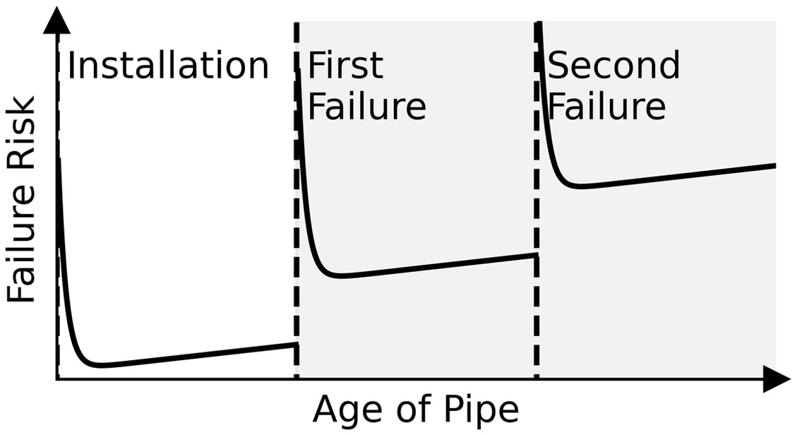
The wide variety of probabilistic pipe break models that have been developed are generally distinguishable by their treatment of how pipe failure risk changes as a function of age and the time between failures. For example, Watson et al. (2004) assumed that the failure risk was constant, while Scheidegger et al. (2013) assumed that the time to the first failure followed a Weibull distribution and that the intervals between all subsequent failures followed an exponential distribution (i.e., a constant risk of failure) (Scheidegger et al. 2015). However, the conceptual failure behavior assumed in each model is not necessarily representative of reality, and the degree to which a proposed theoretical failure model accurately represents the empirical failure behavior may impact the quality of the predictions. Scheidegger et al. (2015) proposed a conceptual model for pipeline failure risk based on expected behavior and previous studies (Fig. 1) but provided limited empirical evidence and mentioned that most statistical models only captured a small part of the expected failure behavior. Here we examine two major features of the proposed conceptual model: the presence of self-excitation and the increase in failure risk as pipes age. Owing to insufficient data, we do not address the initial high-risk so-called bathtub phase, as shown in the white panel in Fig. 1. The objectives of this research were to (1) demonstrate methods to assess whether temporal clustering may be present in water main failure data, (2) apply these methods to a large cohort of water mains, (3) evaluate failure risk as a function of pipe age, (4) introduce a statistical main break model that includes self-excitation, and (5) compare the performance of a variety of published models and investigate the effects of including self-excitation.
Methods
Conceptual Failure Model
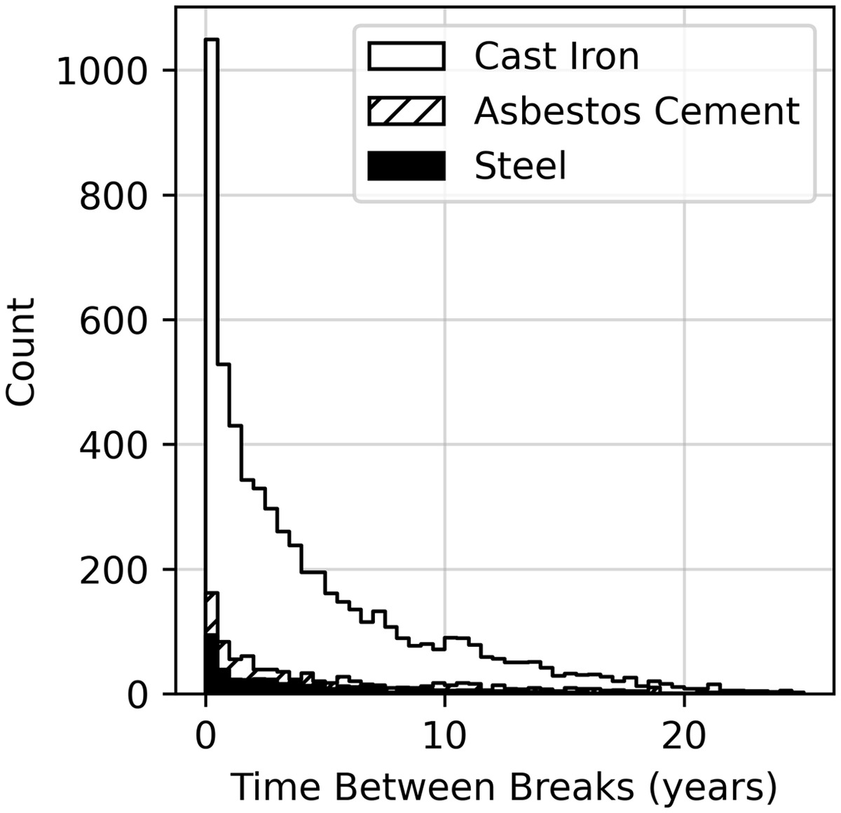
The statistical models considered here explicitly model the failure risk of each pipe segment over time. Conceptual models of failure risk qualitatively describe the expected failure risk experienced by each segment over its lifetime (Fig. 1). The primary conceptual model proposed in the literature is characterized by (1) an initial high-risk period that quickly decreases to a baseline risk level (known as the bathtub phase and shown in the white panel in Fig. 1), (2) a slow and constant increase in break risk with age, (3) an instantaneous increase in break risk with each subsequent failure that decays back to baseline (self-excitation), and (4) a permanent increase in risk following each repair (Scheidegger et al. 2015). Temporal clustering of main breaks may include the effects of self-excitation but may also be caused by other phenomena. Goulter and Kazemi (1988) encountered temporal clustering of main breaks in a water distribution system and quantified the behavior by calculating the marginal temporal failure rates as a function of time since each failure. Clark et al. (1982) also found temporal clustering among mains operated by two separate water utilities. Here we assess temporal clustering in two ways: first, by quantifying the time between breaks on individual pipe segments and visualizing the distribution of the results in a histogram and, second, by calculating the risk of failure as a function of time since the previous break. For each year after a given break, pipes that were not in active service in that year were removed from the cohort of pipes considered.
We evaluate break risk as a function of pipe age by determining the age of each active pipe in each year of the study period and standardize the total number of breaks at each age by the total length of active mains that experienced that age during the period. The results were then grouped into 5-year intervals and averaged. Two procedures were implemented to isolate the effects of aging: (1) only the first known failure on a pipe was considered, and (2) only data for failures occurring 8 years after the first breaks were recorded were used (for more information, see the Supplemental Materials). The bathtub portion of the conceptual failure risk model has been cited in the literature, but without supporting empirical evidence. The main justification for the bathtub portion of the pipe break risk curve is that there may be an initial period when a pipe is installed where defects in manufacturing and installation may lead to a quick failure. After this initial high-risk phase, the risk decreases to typical background levels and then increases with age. Empirical evaluation of this phenomenon is challenging because most water mains were installed long before break records began and because breaks on newly installed pipes are rare. This aspect of the conceptual failure model was not evaluated due to insufficient data.
Failure Modeling
Many different approaches to modeling main breaks have been proposed. The distinctions between models can generally be summarized by considering three characteristics: the smallest unit considered (e.g., individual pipe segments or network-wide), the modeled events (e.g., failure events or the end of pipe’s life), and the modeled process (e.g., physical or statistical) (Scheidegger et al. 2015). Here we restrict our analysis to statistical models, as physical models require intensive data collection that is often not feasible for all but the largest mains (Scheidegger et al. 2015). Scheidegger et al. (2015) noted that many early pipe break models focused on the aggregated behavior of the entire network. However, because pipe replacement strategies generally focus on pipe-level decision making, and because network characteristics can change over time at the pipe level, modeling individual pipes may be much more useful. Although subsections of a network could be modeled to increase the utility of results, performing analyses on spatiotemporal grid cells with aggregated data is vulnerable to a notorious issue known either as the ecological fallacy or the modifiable areal unit problem (MAUP). Reinhart (2018) noted that the MAUP is a serious problem because regression coefficients can depend heavily on the arbitrary boundaries chosen by the analyst. As a consequence, the results are not necessarily trustworthy, and incorrect conclusions might be drawn regarding individual units (Fotheringham and Wong 1991; Openshaw 1984).
Models that analyze individual pipes model either the lifespan or the failure rate of a pipe. According to Scheidegger et al. (2015), lifespan models suffer from inflexibility and are not as useful as failure rate models because the reasons for pipe replacement are not necessarily due to structural deterioration, and thus the results are not generalizable to either other networks or the future of the same network. Pipe failure rate models assume that the breaks experienced by each pipe are generated by a stochastic process based on the assumptions that a pipe can fail anytime while in service, repairs are effectively immediate, and pipes can age and break without limit until they are replaced (Scheidegger et al. 2015). Here we note an additional assumption that is implicit in many studies: the date on which the break is reported is assumed to be the date of failure. Unfortunately, it is difficult to quantify the time elapsed between the occurrence and reporting of a pipe failure.
Missing history is another inescapable aspect of modeling pipe breaks because most of the history takes place before break records were kept. Many models simply acknowledge the associated error, whereas Lin and Yuan (2019) simulated the missing history with data augmentation techniques combined with Markov chain Monte Carlo. One challenge associated with missing failure history is that the form of the log-likelihood typically used for maximum likelihood estimation of the model parameters assumes a complete history. Although the log-likelihood can be modified to account for missing history (Scheidegger et al. 2013), doing so may be impractical for real-world applications. However, the extent to which missing failure history affects the model depends on the model formulation. For example, if the number of previous breaks is included as a covariate, then the majority of pipes in a typical model will be missing key information. While simulating the missing history appears to provide a solution, the computational requirements are high. Alternatively, it may be reasonable to ignore the missing failure data under the working hypothesis that the influence of past failures decays relatively quickly. If this assumption is accurate, the error due to missing history would become negligible except for some small error at the boundary of when break records first began.
To include the self-excitation behavior illustrated in Fig. 1, a model must include a function describing the failure risk that immediately increases when a failure occurs and subsequently decays. For example, Lin and Yuan’s (2019) model raises the time since the last failure to an exponent determined through maximum likelihood estimation. If the exponent is negative, the behavior will be similar to that described in Fig. 1. Alternatively, a self-exciting point process (SPP) would include the increase in risk from all past breaks, not just the most recent. SPP models have been used to model earthquakes, crime, epidemics, and other phenomena where there is reason to believe that events trigger other events in space, time, or both (Reinhart 2018). While the models presented here do not explicitly consider spatial clustering, spatial information is included through a variety of covariates assigned to each pipe segment. Given both the acknowledgment in the literature and the evidence presented here of temporal clustering of main breaks, a SPP model appears to be suited to modeling these events while potentially minimizing error associated with missing break history.
Model Specification
SPPs can be characterized by their conditional intensity function, which estimates the event occurrence rate at any point in space and time. SPPs typically map to two-dimensional Euclidean space, although significant progress has been made recently in their application to linear networks (Baddeley et al. 2021). Because this model applies to a network of pipes whose composition is variable over time (pipes can be installed or abandoned/removed and occupy the same physical location at the same time), the spatial coordinates refer to each unique pipe (), with spatial information associated with each pipe included as covariates. Each unique pipe () consists of a continuous segment of pipe as found in the geospatial pipe data set provided by a water utility. The model presented here is a SPP with pipes , events on pipes with event times (where is the last time step in the study and 0 is the beginning of the study observation window, not the age of the pipe) with event number , time steps , and pipe history . The event times () consist of real numbers and are thus not restricted to the integer domain of the time steps for the time-varying covariates. For example, given a group of five pipes (), one might observe the sequence of breaks shown in Table 1.
| 0 | 2.23 | 0 | 0 |
| 0 | 4.02 | 1 | 4 |
| 2 | 0.40 | 0 | 0 |
| 2 | 2.30 | 1 | 2 |
| 2 | 3.67 | 2 | 3 |
| 4 | 6.91 | 0 | 6 |
| 4 | 7.42 | 1 | 7 |
| 4 | 9.09 | 2 | 9 |
| 4 | 11.34 | 3 | 11 |
The conditional intensity for pipe at time given its history takes the formwith implied hereafter. The background intensity function is shown in Eq. (2), where and are vectors of and parameters, respectively, and and are matrices of time-variant and time-invariant covariates, respectively.
(1)
(2)
The triggering function accounts for the self-excitation of breaks on the same pipe and is commonly specified in the exponential form, i.e., where controls the increase in intensity due to an event and controls the decay (Laub et al. 2015).
(3)
This model assumes a background intensity based on spatiotemporal covariates and a self-exciting triggering intensity that decays exponentially in time, a specification also assumed by Reinhart and Greenhouse (2018), although with the addition of a Gaussian spatial triggering term not considered here.
Parameter Estimation
The parameters of SPP models are estimated by maximizing the log-likelihood, which is adapted from Reinhart and Greenhouse (2018) aswhere ; is the first time step of the study in which pipe is active; and is the last time step of the study in which pipe is active. Maximization is performed using either sequential least-squares programming (SLSQP) or the modified Powell algorithm as implemented in the Python package SciPy (Virtanen et al. 2020). As noted earlier, the expression for the log-likelihood given by Eq. (4) assumes that the complete break history is known (Reinhart 2018). To improve problem solvability and for consistency with the conceptual model shown in Fig. 1, and were limited to positive nonzero values.
(4)
Parameter Inference
Confidence intervals for the fitted parameters were produced with the asymptotic covariance matrix estimatorwhere the list of all is the list of all failure events (with more than one entry per when a main has broken more than once); the value of is the pipe identification number; and the matrix-valued function has rows and columns (where and refer to a given parameter within ) and is given by
(5)
(6)
This method was suggested by Rathbun (1996) and used by Reinhart and Greenhouse (2018). There are two other options for obtaining confidence intervals: (1) calculating the Hessian of the log-likelihood and (2) a parametric bootstrap method. The bootstrap approach is computationally intractable for large data sets, and the Hessian method was not as robust as using Rathbun’s estimator in Reinhart’s analysis (Reinhart and Greenhouse 2018). The 95% confidence intervals for the parameter estimates are produced by multiplying the estimated standard errors by a critical value of 1.96 (Hazra 2017). We assume that regularity conditions apply: the true parameters must be interior to the parameter space, the log-likelihood function must be thrice differentiable, and the third derivatives must be bounded.
Model Selection
Model selection was performed by fitting the model with all available covariates and subsequently removing those covariates with the most uncertain coefficients based on a Wald test (Agresti 2007). Parameters whose estimates have -values less than 0.1 are included in the model.
Comparison Models
Several published models were evaluated and compared to the proposed SPP model using identical estimation and simulation procedures and covariates. The model given by Scheidegger et al. (2013) assumes the time to the first failure is Weibull distributed, while the subsequent failures are assumed to follow a single exponential distribution. The conditional intensity for this model, modified to include covariates following Scheidegger et al. (2015), is given bywhere is the previous number of breaks at time . Scheidegger et al. (2013) modified the maximum likelihood estimation to account for missing pipes; however, the same maximum likelihood estimation approach is used here for all models to ensure the comparisons are valid. While Scheidegger et al. (2013) used Bayesian methods, the data sets used here are sufficiently large to allay concerns over discrepancies between the two approaches. Unfortunately, significant missing failure history means that an assumption is required to implement Scheidegger et al.’s (2013) model: the first observed failure is assumed to be the first failure [i.e., ].
(7)
Kleiner and Rajani (2010) implemented a nonhomogeneous Poisson model that is essentially the same as the SPP model but with a constant parameter () and without the triggering function. Their model is given by
(8)
Lin and Yuan (2019) proposed a type of two-time-scale point process model that incorporates covariates, pipe age (included here in ), and time since the last break in a conditional intensity function similar in form to
(9)
We assume that if there are no previous breaks, then the term accounting for break history has a value of 1.
To evaluate the performance of the models with and without self-excitation, modifications were made as follows. Scheidegger et al.’s (2013) model was compared with and without the triggering function shown in Eq. (3). Kleiner and Rajani’s (2010) model was compared with the SPP model because they are nearly identical aside from the inclusion of self-excitation in the SPP model. Lin and Yuan’s (2019) model was compared with and without its original self-excitation function as shown in the right half of Eq. (9).
Performance Evaluation
Simulation and Forecast
Simulations of failure events were obtained by implementing the method outlined in Section 5 in Zhuang et al. (2004), which involves first generating a background catalog of events based on the specified background intensity () and subsequently generating the so-called children for each generation of events based on the specified triggering function’s () normalized probability density function. The background nonhomogeneous stationary Poisson process was generated using Lewis’s thinning algorithm (Lewis and Shedler 1979; Zhuang and Touati 2019). Rather than simulating the break behavior for all pipes over the entire study period in a single simulation, which could lead to error propagation, the method used here draws upon the approach given by Algorithm B in Section 3.3 of Zhuang (2011) and simulates breaks in a stepwise fashion, with the true break history used to simulate future breaks. For example, given the true break history up to, but not including, time , the break behavior for was simulated using the true break history and the method outlined earlier. The training period consisted of monthly stepwise simulations performed until January 2018. The rest of the study period (from January 2018 through December 2020) was used as a single forecasting period (i.e., the testing period). The same simulation procedure was used for all models. However, the algorithm used to generate the children was only implemented where the triggering function is additive [e.g., see Eq. (1)]. Further details regarding the simulation algorithm may be found in the Supplementary Information.
Pipe-Level Predictions
In addition to providing information on factors related to pipe breaks, the models presented here provide additional information in the form of pipe-level break probabilities. Each simulation based on a fitted model is a realization of the modeled stochastic process for each pipe segment. Whether or not a given pipe breaks in each simulation depends on its conditional intensity over the forecasting period (break probability) and the randomness of the simulation. Thus, when many simulations are run over a certain time period (i.e., a Monte Carlo simulation), the pipes that are simulated as breaking are likely to break only in some fraction of those simulations. If a pipe breaks in 60% of the simulations, it is assigned a break probability of 0.6. This value may be used to classify the pipe segment as either breaking or not breaking during the forecast interval, depending on the classification threshold. This information may be useful to water utilities seeking accurate, pipe-level predictions for pipeline replacement programs. The pipe break predictions from the training period were not used for this aspect of the analysis.
Classifiers are often evaluated using receiver operating characteristic (ROC) curves, which plot the true positive rate versus the false positive rate. However, ROC curves are flawed measures of classification performance when the data are highly imbalanced (i.e., a small number of positives versus negatives) (Lever et al. 2016). Because main breaks are rare when considering the total number of pipes that are active within a distribution system, precision-recall (PR) curves are more appropriate for measuring the performance of a main break classifier. In plots of precision versus recall, superior classifiers produce curves closer to the top right. The area under the PR curve (AUC-PR) is a way to quantify the relative performance of each classifier, with greater AUC-PR indicating better performance. A random classifier will result in an AUC-PR approximately equal to the positive rate in the sample (Sofaer et al. 2018). AUC-PR values were calculated using the trapezoidal rule as implemented in the Python package NumPy (Harris et al. 2020).
Data
Distribution Network and Main Breaks
The distribution network and main break data used for this analysis were provided by East Bay Municipal Utility District (EBMUD), a water agency serving 1.4 million customers in California, USA. Main break data were provided in the form of a geospatial data set containing the location and date reported for each break in addition to the attributes of the pipe on which the break occurred, the failure mode, comments by the maintenance crew, and other identifying information. Additionally, a geospatial pipeline database was provided that gives the location and attributes of each pipe, here defined as the unit of pipe assigned a unique identification number by EBMUD in the provided data sets, including material, diameter, length, installation year, life cycle status, life cycle status change date, pressure zone, and others. However, there is no direct link between the main break data set and the provided pipeline data set, meaning we cannot assign breaks to pipes with full certainty. This means that the two data sets, one for breaks and one for mains, must be combined to obtain the best available estimate of the break history for each pipe segment and to infer missing pipes.
To obtain the best available estimate of each pipe’s break history, an automated algorithm was used to match breaks to pipes and if necessary infer pipes based on the available evidence. EBMUD has confidence in the geospatial fidelity of the mains to within approximately , and the main breaks are associated with the nearest address. The laterals, which connect mains and service connections (with addresses), were used to adjust the locations of the main breaks to overlap the mains. The main breaks were then assigned to the most likely nearest pipe based on matching pipe characteristics, for example, the estimated installation year and pipe material. If no suitable pipe was found for a given main break, a main was inferred based on the estimated pipe characteristics found in the main break records.
Installation practices vary based on the type of cover (e.g., asphalt versus soil only) and the type of road (e.g., highway versus local street) under which the pipe is located. To reduce variability among the pipes considered for modeling, only pipes adjacent to or buried under local streets were used. Local streets were defined as roads bearing a Caltrans Functional Classification System value of 7. This group of pipes is the largest in EBMUD’s distribution network (76% by length). Additionally, only main breaks assigned the highest priority levels of 4 and 5 (91% of all main breaks) were modeled. EBMUD assigns priority from 1 to 5 to each break based on severity (with priority 5 breaks most severe). This is intended to mitigate the error associated with breaks that are reported long after they actually occur, which may be more likely for breaks of lower severity. For example, a catastrophic main break (likely priority five) is more likely to be immediately noticed and reported by the public than a very small leak (likely a much lower priority). The lag time between the date a break is reported and the date the break actually occurred is of great interest to utilities and could be included in the model by adjusting break times as necessary. However, this is a difficult problem to solve, and since no solution has been found, it must be accepted as contributing to the error of any pipe break model.
Missing Pipe and Break Data
Several common deficiencies of distribution network and break history data must be resolved for modeling to proceed. Two widespread issues are left truncation and survival bias (Scheidegger et al. 2015). The first consists of missing break history, which is an inescapable flaw of main break data collected by most water utilities that began operating long before the digital age. This is especially relevant for EBMUD given that pipes were installed in its service territory as early as 1866, while digital break records only go back to 1997. This means that of the approximately 155 years over which main breaks have occurred, records only exist for approximately 23 years, or 15%.
While Lin and Yuan (2019) simulated the missing history, pipe break modelers often choose to ignore this problem by assuming no dependence on past breaks or by including a variable accounting for the number of known breaks. The relevant question is whether or not the missing break history is important and, if so, to what extent. For the SPP model, instead of including the total number of breaks experienced by a pipe at any given time, the effect of past break history is described by the triggering function [Eq. (3)]. Problems arise when events are triggered by an event outside of the temporal boundary, but the magnitude of this problem can be assessed though the triggering parameters and estimating the duration that the temporary increase in risk due to a break is significant. The data shown in Fig. 2 suggest that the self-excitation effect is relatively short, on the order of approximately 5 to 15 years depending on the material. This suggests that the missing break history beyond a few years near the boundary will have minimal impact on the model and can be safely neglected. The error due to the missing break history near the temporal boundary is accepted as a minor source of error. This is a common approach in earthquake and crime modeling, where an additional assumption must also be made about events being triggered from outside the spatial boundaries.
The second issue (survival bias) is the absence of information about abandoned or replaced pipes in the database of pipes, which means that only pipes that have survived are observed. Because the surviving pipes may not be representative of the entire cohort, the results of analyses using only surviving pipes may not be generalizable. Fortunately, EBMUD’s records contain information on many abandoned or removed pipes. The remaining error due to this flaw in the data is partially mitigated by inferring the presence of missing pipes using the break data. The algorithm that assigns each break to a single pipe segment also flags breaks with no satisfactory pipe assignment. Using the pipe characteristics associated with the flagged break, the missing pipe is generated and is assumed to be collocated with the nearest pipe segment. However, this procedure does not mitigate the error associated with missing data on pipes that were abandoned before digital records began or pipes that were abandoned after digital records began but did not fail during that time period and were not kept in the pipe database. For more information on the break-pipe assignment algorithm, see the Supplementary Information.
Weather Data
Air temperature and precipitation data were obtained from the National Oceanic and Atmospheric Administration Global Historical Climatology Network (Menne et al. 2018) and the stations used for this analysis are all those within 16.1 km (10 mi) of the pressure zones operated by EBMUD. There are 15 temperature stations within 16.1 km (10 mi) of the service territory. Only nine of those have full coverage of the study period, and the others are fairly sparse. The missing data were filled with that station’s nearest neighbor data. The same approach was used for the 88 stations with precipitation data within 16.1 km (10 mi) of EBMUD’s service territory, many of which do not have complete records. Each pipe was assigned the weather data of the nearest station.
Traffic and Roadways
GIS data for California’s roads were obtained through the freely available Functional Classification data set published by Caltrans (2021). Each pipe was assigned the type of road to which it is nearest, which consists of a value of 1 (interstate), 2 (other freeway or expressway), 3 (principal arterial), 4 (minor arterial), 5 (major collector), 6 (minor collector), or 7 (local). Additionally, monthly geospatial traffic volume (estimated trip counts) data were obtained from StreetLight Data (San Francisco, California, USA) spanning from 2018-07-01 through 2020-01-31 (the date format used in this work is YYYY-MM-DD in accordance with ISO 8601). Owing to the number of pipe segments studied, obtaining unique traffic data for each pipe is not feasible. Thus, the traffic data were aggregated to spatiotemporal grid cells and normalized by the area of the cell. The cells were designed to minimize misrepresentation of the traffic experienced by each pipe by isolating high-traffic roads within their own polygons. The polygons were generated using Voronoi tessellation and manual modification as necessary to include all pipes and to meet the maximum polygon limit imposed by Streetlight. The traffic data contain distinctions for pass-through, end-in, and start-in traffic. The pass-through traffic is distinct from the other types and may be attributed to arterials and freeways rather than local roads. Accordingly, pipes under local roads were assigned the traffic volume values from the start-in and end-in categories. In addition to the time-varying traffic covariate, a per-pipe aggregated value was also included under the assumption that the value is valid beyond the dates for which traffic data are available. All traffic covariates are normalized by the area of the grid cell to which they belong.
Soil Data
Soil data were obtained from the USGS gNATSGO (Soil Survey Staff 2021) data set and assigned to each pipe using ArcMap (Esri, Redlands, California, USA). Unfortunately, soil properties cannot be assigned to all pipes due to the incomplete coverage of EBMUD’s service territory. Soil clay content, electrical conductivity, and pH are available for 95%, 71%, and 76% of the mains, respectively. When these variables were included, the pipes without data were ignored.
Water Demand Data
Monthly water demand data were provided by EBMUD for all of its customers from 2005-01-01 through 2021-01-31. The addresses were geolocated and used to assign a local demand surrogate for each pipe. To capture all pipes using this method, the 50 nearest customer taps within a 16.1 km (10 mi) radius of each pipe were used to calculate the time-varying demand surrogate. Additionally, a single, all-time average per-pipe surrogate demand value was included as a time-invariant covariate to characterize the general demand trends for each pipe and to isolate the fluctuations of demand over time. A very small group of pipes (0.34% of all pipes) has much greater surrogate water demand than most other pipes. These pipes are considered outliers or not representative and were excluded from modeling.
Results and Discussion
Descriptive Analysis
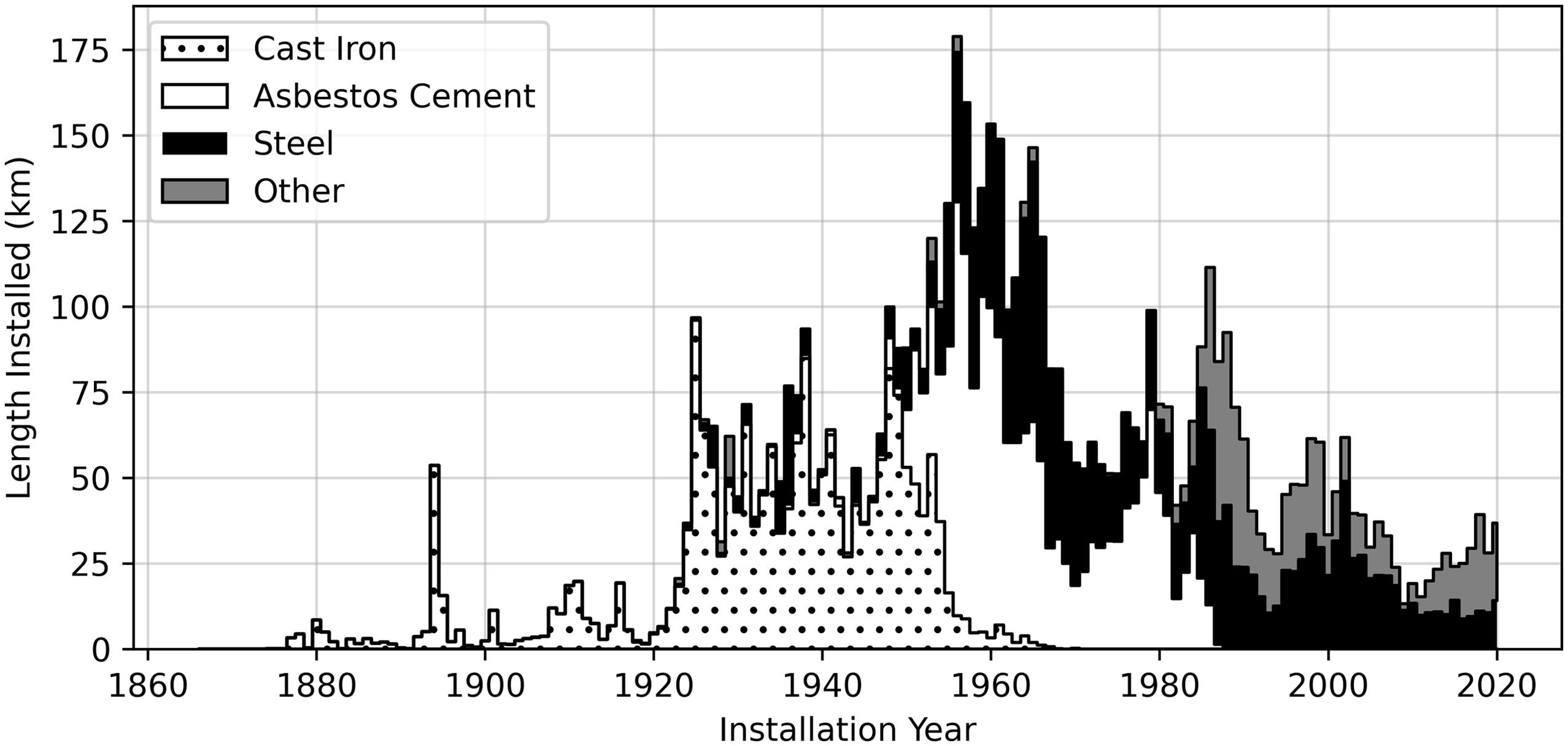
The active distribution network (as of 2020) consists of approximately 6,677 km (4,149 mi) of mains consisting of 30.2% cast iron (CI), 27.4% asbestos cement (AC), 31.1% steel (ST), and 11.3% other material types (by length), as shown in Fig. 3. Out of the total number of mains used for modeling (200,300 CI, AC, and ST mains, including both provided and inferred pipe segments) and considering the years 1997 through 2020, approximately 5% have experienced at least one break, 1.8% have experienced at least two breaks, and 0.8% have experienced three or more breaks. The highest number of breaks on any one pipe is 19. The average main pipe segment length is 36.9 m (121 ft), 38.7 m (127 ft), and 32.6 m (107 ft) for CI, AC, and ST, respectively. Diameters vary by pipe material type as shown in Fig. S1 . The network has experienced at least 25 main breaks per month since 1997, with a distinct bimodal seasonal distribution of breaks with a peak in the winter and a peak in late summer/fall, as shown in Fig. S2 , which suggests that there are underlying seasonal factors involved. To better characterize the seasonality of main breaks, it is essential to separate the breaks by pipe material and failure mode. The material properties of CI and ST are different than those of AC and accordingly we see differences in seasonal behavior. EBMUD records the failure mode of each break as a circumferential, longitudinal, blowout, or joint failure. The failure mode provides information on the types of stresses that may have caused the break. Fig. S3 shows how the main breaks studied here are allocated among different material types and failure modes. There were 17,433 main breaks from 1997-01-01 through 2021-07-31, with the most belonging to CI (73.4%), AC (18.2%), and ST (7.3%) mains. From 2013-01-01 through 2020-12-31, reported main breaks occurred at an average rate of 21 breaks per 161 km (100 mi) per year for all breaks, and 49, 16, and 4 breaks per 161 km (100 mi) per year for CI, AC, and ST mains, respectively. Separating the breaks by material reveals that CI maintains the bimodal seasonality while AC exhibits a single peak in the summer and ST shows only a slight increase in the winter, as shown in Fig. S4 .
Further separating the breaks by failure mode shows that CI’s bimodal seasonal pattern shown in Fig. S4 results from superimposing the unimodal seasonal patterns observed for circumferential breaks and longitudinal splits, as shown in Fig. S5 . The circumferential breaks account for most of the winter peak and are the most numerous. Longitudinal splits and blowouts are the next most common type of break, while joint failures are the least common. Longitudinal splits peak in the summer, while blowouts show a slight bimodal behavior with a larger peak in the summer and joint failures appear to peak only in summer. AC mains demonstrate a clear tendency to break more frequently during the summer months. This trend is primarily driven by circumferential breaks and blowouts, as shown in Fig. S6 , while longitudinal splits and joint failures display little to no seasonality. ST pipe breaks exhibit very little seasonality, as shown in Fig. S7 . For additional discussion on the seasonality of main breaks, see the Supplemental Materials.
Conceptual Model
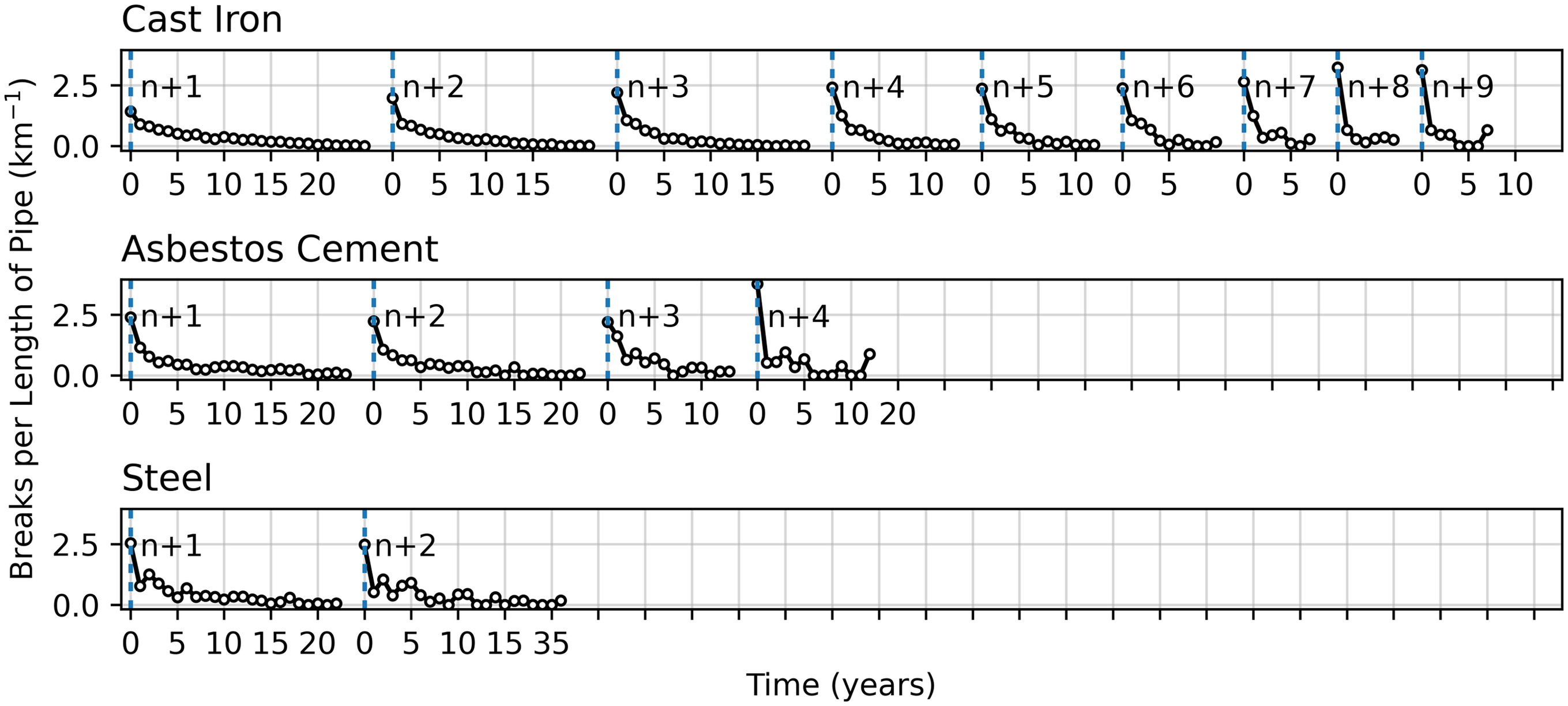
The distribution of interevent times for failures on individual pipes is shown in Fig. 2. If the risk of failure was constant, the histogram would resemble an exponential distribution. Because the histogram’s bars do not exhibit geometric decay (i.e., a constant ratio between adjacent bars), the distribution does not appear to be exponential. Thus, the strong positive skew shown in Fig. 2 appears to provide evidence of temporal clustering, which may include self-excitation. Another way to investigate temporal clustering is by estimating the risk of failure as a function of time. Fig. 4 shows how the break risk evolves as a function of time since the previous break and the number of breaks on each pipe. For CI it appears that with each subsequent break, the increase in break risk is greater than the previous increase. Fig. 4 also shows that the amount of time required for CI break risk to decay back to baseline becomes shorter as the number of breaks increases from the initial value of (where is the number of breaks experienced by the pipe before records began). The general trend is the same for AC mains, but less extreme. It appears that the difference in break risk between and breaks is not significant for AC or ST. A caveat of this analysis is that the value of is unknowable for the vast majority of pipes in the available database because they were installed before records began. However, the results suggest that models that include self-excitation may be appropriate for the data used here.
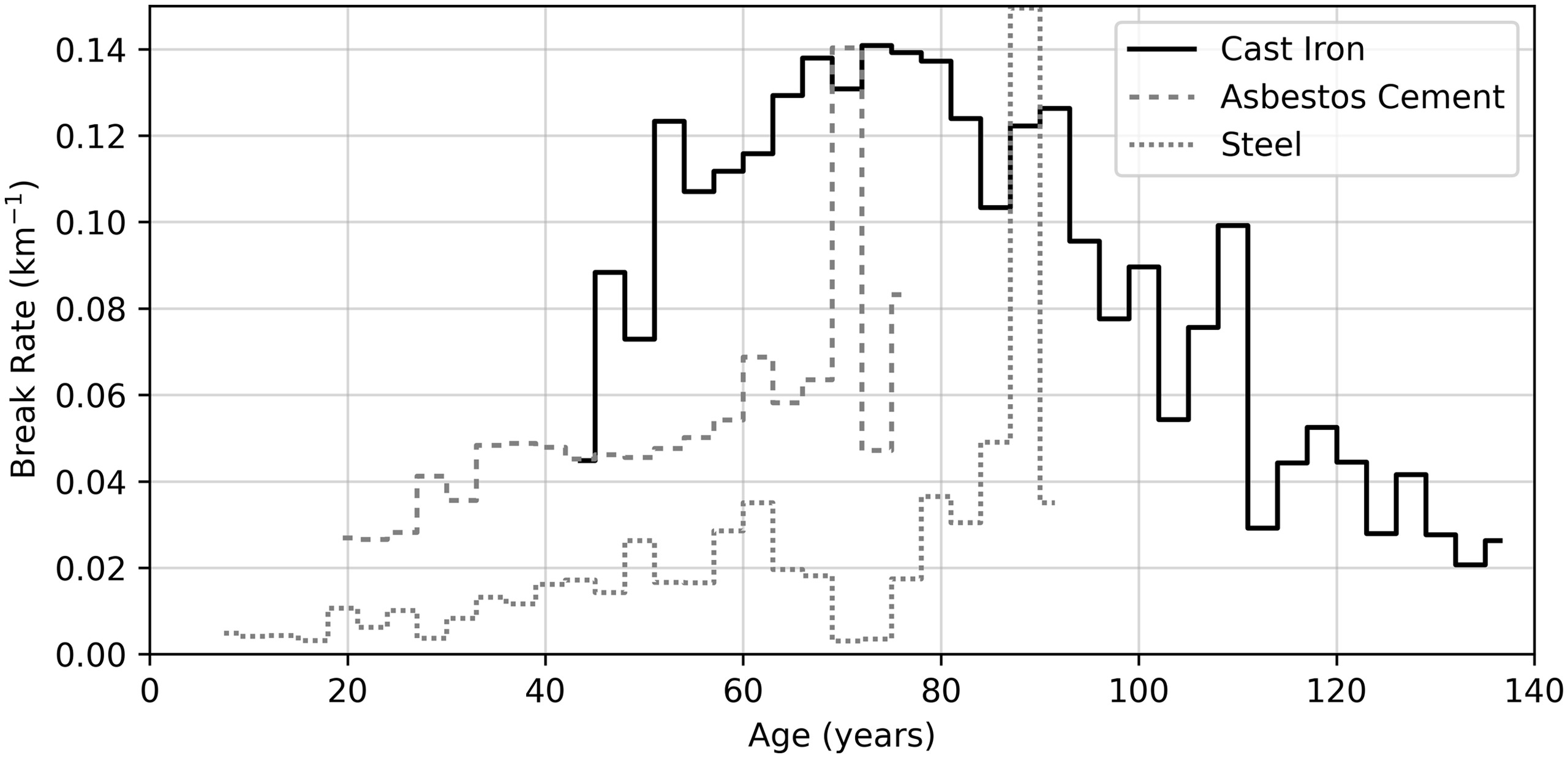
Another assumption of the conceptual model shown in Fig. 1 is that break risk increases monotonically with age. Intuition suggests that as pipes get older and experience adverse conditions and stressors, their risk of failure should increase. The empirical failure risks for CI, AC, and ST mains as a function of age are shown in Fig. 5. While the empirical failure risk does increase consistently for CI until approximately 70 years of age, the risk subsequently decreases significantly. Although the overall trends for both AC and ST indicate that break risk increases with age, both cohorts of pipes are much younger than the group of CI pipes, some of which reached nearly 140 years of age during the study period. As the AC and ST mains age, they may see decreases in failure rates similar to those of CI mains. Le Gat (2014) also investigated the empirical failure rate of a large cohort of pipes (steel core concrete pipes) and found that the failure rate did not increase monotonically. Le Gat (2014) did not observe a significant decrease in failure rate with extreme age, but the data were limited to only pipes younger than 80 years of age. This evidence suggests that assuming break risk increases monotonically with age may not be appropriate in all cases. However, the decrease in risk observed in CI mains may be due to a combination of both physical and artificial factors, including survival selection in the population of pipes, mild environmental conditions, and variability in the manufacturing process. The oldest CI pipes, those fabricated before 1920, were constructed using sand pit casting, which resulted in greater variations in wall thickness than found in more modern centrifugally spun CI pipes (Talbot 1926). Perhaps the CI mains still in use today are resilient due to variations in the manufacturing process that resulted in some pipes being more durable than others. Alternatively, the trend observed here may be an artifact of incomplete data and survival selection.
Statistical Modeling
Estimation and Inference
The estimated model parameters are shown in Table S7 . The coefficients may be interpreted relative to each other within each material type because the covariates were all scaled to the same range (between 1 and 2). The self-excitation parameters were statistically significant (95% confidence level) in all cases, suggesting that the observed temporal clustering could be described by self-excitation. Traffic volume was evaluated as a time-varying covariate to the extent permitted by data availability, which was limited to 2018-07-01 to 2020-01-31. Traffic volume failed to produce a significant parameter estimate at the 95% confidence level, with the exception of traffic for CI main breaks. Traffic appears to be significant for CI main breaks at the 95% confidence level, but the resulting coefficient is negative. This implies that increased traffic is associated with reduced break risk. Although unintuitive, this result is consistent with findings by Eisenbeis (1994). To facilitate comparison between material types and to take advantage of the longer time span available for other covariates, traffic was removed from consideration, and the study proceeded with the full set of covariates available from 2013-01-01 through 2020-12-31, as shown in Table S7 . Some results are intuitive, including the negative coefficients for diameter (larger-diameter pipes are stronger due to their larger area moment of inertia), positive coefficients for length (longer pipes present more opportunities to break), the positive coefficients for soil clay content (higher clay contents result in more extreme soil expansion and contraction), and the positive coefficient for air temperature for AC mains (in the study area, higher temperatures coincide with arid conditions in which differential soil settlement occurs due to variations in moisture content). Contrastingly, the negative coefficient for the age of the pipe for CI and AC mains is unintuitive when considering only the conceptual failure model described earlier. However, the empirical failure risk shown in Fig. 5 suggests that any single coefficient for age may be inadequate, as failure risk does not necessarily increase monotonically with age. For an extended discussion of the estimation and inference results, see the Supplemental Materials.
Network-Wide Forecasting
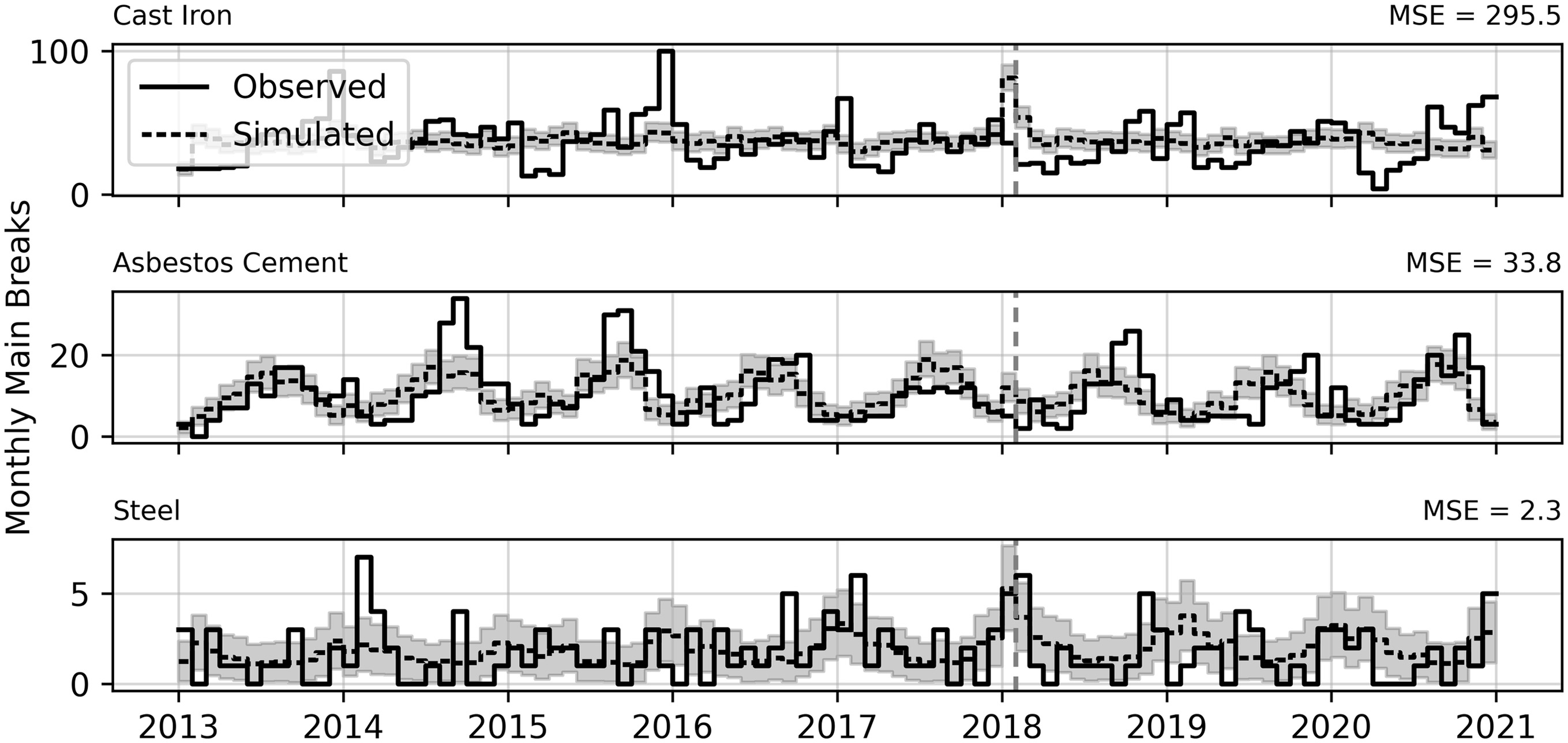
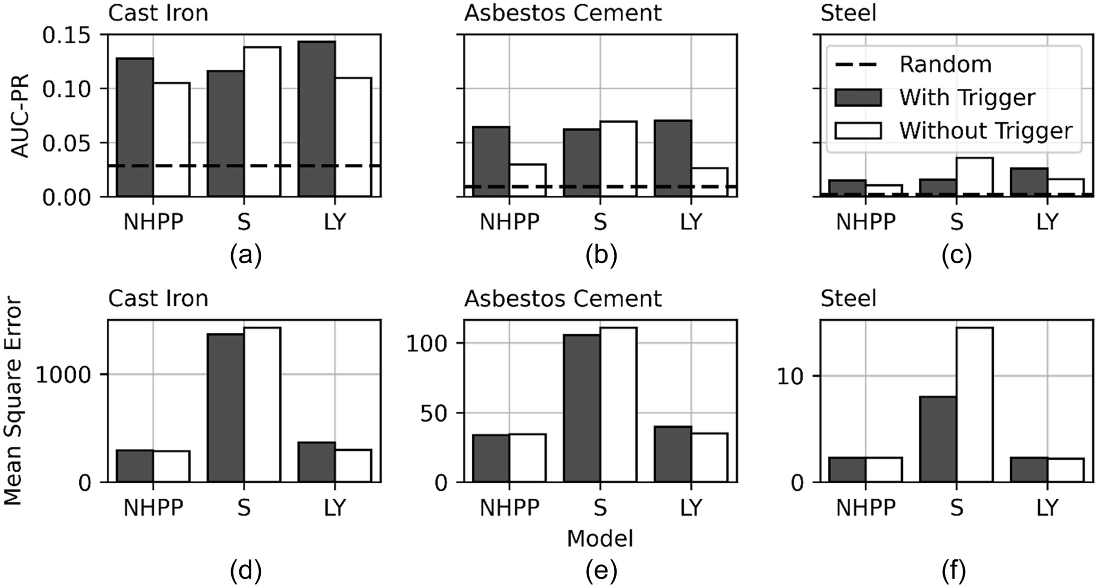
The network-wide predictions resulting from the SPP model fitted to CI, AC, and ST main breaks are compared to the observed data in Fig. 6. The models for CI and ST capture the average break behavior, while the model for AC better describes the seasonal variation in breaks. As suggested by the different seasonal trends shown in Fig. S5 , CI breaks are likely driven by many different factors. The models presented here do not distinguish between the failure modes, and thus the relationships between covariates and main breaks may be different for different types of breaks. This may explain why the simulated seasonal behavior is damped for the CI model. Conversely, the majority of AC main breaks appear to be correlated with a single seasonal variable, as shown in Fig. S6 . Accordingly, the simulations show good agreement with the observed seasonal patterns of AC main breaks. ST main breaks do not display obvious seasonal patterns and appear to be much more random than their CI or AC counterparts, and the fitted model for ST breaks reflects this lack of seasonality (Fig. S7 ). The network-wide main break predictions resulting from Scheidegger et al.’s (2013), Lin and Yuan’s (2019), and Kleiner and Rajani’s (2010) models are shown in Figs. S8 –S10 . Kleiner and Rajani’s (2010) model resulted in the lowest mean square error (MSE) for CI, followed closely by the SPP model and Lin and Yuan’s (2010) model. For AC, the SPP model provided the lowest MSE, while Lin and Yuan’s (2019) model provided the lowest MSE for ST. It appears that including self-excitation resulted in higher MSEs in some cases while reducing MSEs in others (Fig. 7).
Pipe-Level Predictions
The PR curves for all six models (three with and three without triggering functions to model self-excitation) are shown in Fig. S11 . The AUC-PR for all models are summarized in the top row of Fig. 7. A larger AUC-PR indicates better classification performance. The data suggest that only Scheidegger et al.’s (2013) model is superior without triggering and that predictions of CI main breaks are superior to predictions of AC and ST main breaks. It appears that although self-excitation is observed in the empirical data, including it in the model definition does not always improve failure predictions. Moreover, the second-highest performing model across all materials (based on Fig. 7), Scheidegger et al.’s (2013) original model (without self-excitation), performs nearly as well as Lin and Yuan’s (2019) model with self-excitation. The significant additional computational effort to include triggering may not be worth the small difference in classification performance between the two models. Interestingly, the models that proved superior at classifying individual failures were not necessarily better at predicting network-wide behavior. For example, as shown in Fig. 7, Scheidegger et al.’s (2013) model applied to CI, AC, and ST failures was nearly the best at classifying individual breaks (according to the AUC-PR) but in all cases produced larger MSEs for network-wide predictions compared to the other models.
Significance of This Work
Conceptual models of water main failure risk should be supported by empirical evidence, as they may play an important role in future model development. The data presented here suggest that self-excitation may occur in CI, AC, and ST water mains. Practitioners should investigate the cohort of pipes they wish to model to check for the validity of their modeling assumptions. However, this work also suggests that even if self-excitation may be present, adding self-excitation to an existing model may not improve the results. Furthermore, models that give good single-pipe failure classification results may not provide good network-wide simulations. Thus, because the effectiveness of the model will directly affect whether resources are used efficiently, a variety of models should be evaluated to determine which is most suitable for the desired outcome. This work also illustrates the observed seasonal variation of main breaks in a Mediterranean climate and provides statistical inference results for a variety of relevant covariates that may be of use to practitioners in guiding further investigations. Further research based on these results could include developing models that distinguish between failure modes, describe break risk as a function of age more accurately, and account for changes in self-excitation behavior over time.
Supplemental Materials
File (supplemental materials_jwrmd5.wreng-6432_hammond.pdf)
- Download
- 1018.71 KB
Data Availability Statement
Some or all data, models, and code that support the findings of this study are available from the corresponding author upon reasonable request.
Acknowledgments
Many thanks to Alex Reinhart, Adrian Baddeley, Ege Rubak, and Rolf Turner for advice regarding point process modeling. Thanks to Yoni Ackerman for providing technical assistance. Thanks to Nicholas Reseburg (EBMUD) for GIS data assistance. Jiancang Zhuang was partially supported by Grants-in-Aid No. 19H04073 for Scientific Research from the Japan Society for the Promotion of Science (JSPS). This study was funded by East Bay Municipal Utility District under Agreement 2017-450-D. Any opinions, findings, and conclusions expressed in this work are those of the authors and do not necessarily reflect the views of the funding agency.
References
Agresti, A. 2007. An introduction to categorical data analysis. 2nd ed. Hoboken, NJ: Wiley.
Baddeley, A., S. R. Gopalan Nair, G. McSwiggan, and T. M. Davies. 2021. “Analysing point patterns on networks—A review.” Spatial Stat. 42 (Apr): 100435. https://doi.org/10.1016/j.spasta.2020.100435.
Barton, N. A., S. H. Hallett, S. R. Jude, and T. H. Tran. 2022. “An evolution of statistical pipe failure models for drinking water networks: A targeted review.” Water Supply 22 (4): 3784–3813. https://doi.org/10.2166/ws.2022.019.
Caltrans. 2021. “CRS—Functional classification.” Accessed October 1, 2021. https://gisdata-caltrans.opendata.arcgis.com/datasets/cf4982ddf16c4c9ca7242364c94c7ad6_0/about.
Clark, R. M., C. L. Stafford, and J. A. Goodrich. 1982. “Water distribution systems: A spatial and cost evaluation.” J. Water Resour. Plann. Manage. Div. 108 (3): 243–256. https://doi.org/10.1061/JWRDDC.0000257.
Eisenbeis, P. 1994. “Modélisation statistique de la prévision des défaillances sur les conduits d’eau potable.” Doctoral dissertation, Dept. of Civil Engineering, Louis Pasteur Univ.
Folkman, S. 2018. “Water main break rates in the USA and Canada: A comprehensive study.” In Mechanical and aerospace engineering faculty publications. Logan, UT: Utah State Univ.
Fotheringham, A. S., and D. W. S. Wong. 1991. “The modifiable areal unit problem in multivariate statistical analysis.” Environ. Plann. A 23 (7): 1025–1044. https://doi.org/10.1068/a231025.
Goulter, I. C., and A. Kazemi. 1988. “Spatial and temporal groupings of water main pipe breakage in Winnipeg.” Can. J. Civ. Eng. 15 (1): 91–97. https://doi.org/10.1139/l88-010.
Harris, C. R., K. Jarrod Millman, S. J. van der Walt, P. V. Ralf Gommers, and E. W. David Cournapeau. 2020. “Array programming with NumPy.” Nature 585 (7825): 357–362. https://doi.org/10.1038/s41586-020-2649-2.
Hazra, A. 2017. “Using the confidence interval confidently.” J. Thorac. Dis. 9 (10): 4124–4129. https://doi.org/10.21037/jtd.2017.09.14.
Kleiner, Y., and B. Rajani. 2010. “I-WARP: Individual water main renewal planner.” Drinking Water Eng. Sci. 3 (1): 71–77. https://doi.org/10.5194/dwes-3-71-2010.
Laub, P. J., T. Taimre, and P. K. Pollett. 2015. “Hawkes processes.” Preprint, submitted July 10, 2015. https://arxiv.org/abs/1507.02822.
Le Gat, Y. 2014. “Extending the yule process to model recurrent pipe failures in water supply networks.” Urban Water J. 11 (8): 617–630. https://doi.org/10.1080/1573062X.2013.783088.
Lever, J., M. Krzywinski, and N. Altman. 2016. “Points of significance: Classification evaluation.” Nat. Methods 13 (8): 603–604. https://doi.org/10.1038/nmeth.3945.
Lewis, P. A. W., and G. S. Shedler. 1979. “Simulation of nonhomogeneous poisson processes by thinning.” Nav. Res. Logist. 26 (3): 403–413. https://doi.org/10.1002/nav.3800260304.
Lin, P., and X. X. Yuan. 2019. “A two-time-scale point process model of water main breaks for infrastructure asset management.” Water Res. 150 (Mar): 296–309. https://doi.org/10.1016/j.watres.2018.11.066.
Menne, M. J., C. N. Williams, B. E. Gleason, J. Jared Rennie, and J. H. Lawrimore. 2018. “The global historical climatology network monthly temperature dataset, version 4.” J. Clim. 31 (24): 9835–9854. https://doi.org/10.1175/JCLI-D-18-0094.1.
Openshaw, S. 1984. “Ecological fallacies and the analysis of areal census data.” Environ. Plann. A 16 (1): 17–31. https://doi.org/10.1068/a160017.
Rathbun, S. L. 1996. “Asymptotic properties of the maximum likelihood estimator for spatio-temporal point processes.” J. Stat. Plann. Inference 51 (1): 55–74. https://doi.org/10.1016/0378-3758(95)00070-4.
Reinhart, A. 2018. “A review of self-exciting spatio-temporal point processes and their applications.” Stat. Sci. 33 (3): 299–318. https://doi.org/10.1214/17-STS629.
Reinhart, A., and J. Greenhouse. 2018. “Self-exciting point processes with spatial covariates: Modelling the dynamics of crime.” J. R. Stat. Soc. Ser. C 67 (5): 1305–1329. https://doi.org/10.1111/rssc.12277.
Scheidegger, A., J. P. Leitão, and L. Scholten. 2015. “Statistical failure models for water distribution pipes—A review from a unified perspective.” Water Res. 83 (Oct): 237–247. https://doi.org/10.1016/j.watres.2015.06.027.
Scheidegger, A., L. Scholten, M. Maurer, and P. Reichert. 2013. “Extension of pipe failure models to consider the absence of data from replaced pipes.” Water Res. 47 (11): 3696–3705. https://doi.org/10.1016/j.watres.2013.04.017.
Shortridge, J. E., and S. D. Guikema. 2014. “Public health and pipe breaks in water distribution systems: Analysis with internet search volume as a proxy.” Water Res. 53 (Apr): 26–34. https://doi.org/10.1016/j.watres.2014.01.013.
Sofaer, H. R., J. A. Hoeting, and C. S. Jarnevich. 2018. “The area under the precision-recall curve as a performance metric for rare binary events.” Methods Ecol. Evol. 10 (4): 565–577. https://doi.org/10.1111/2041-210X.13140.
Soil Survey Staff. 2021. “Gridded national soil survey geographic (gNATSGO) database for California.” Accessed December 14, 2021. https://nrcs.app.box.com/v/soils.
Talbot, A. N. 1926. “Strength properties of cast iron pipe made by different processes as found by tests.” J. Am. Water Works Assoc. 16 (1): 1. https://doi.org/10.1002/j.1551-8833.1926.tb13414.x.
Virtanen, P., T. E. Ralf Gommers, M. H. Oliphant, D. C. Tyler Reddy, and E. Burovski. 2020. “SciPy 1.0: Fundamental algorithms for scientific computing in python.” Nat. Methods 17 (3): 261–272. https://doi.org/10.1038/s41592-019-0686-2.
Watson, T. G., C. D. Christian, A. J. Mason, M. H. Smith, and R. Meyer. 2004. “Bayesian-Based pipe failure model.” J. Hydroinf. 6 (4): 259–264. https://doi.org/10.2166/hydro.2004.0019.
Zhuang, J. 2011. “Next-day earthquake forecasts for the Japan region generated by the ETAS model.” Earth Planets Space 63 (3): 207–216. https://doi.org/10.5047/eps.2010.12.010.
Zhuang, J., Y. Ogata, and D. Vere-Jones. 2004. “Analyzing earthquake clustering features by using stochastic reconstruction.” J. Geophys. Res. 109 (May): 5. https://doi.org/10.1029/2003JB002879.
Zhuang, J., and S. Touati. 2019. Stochastic simulation of earthquake catalogs, community online resource for statistical seismicity analysis. Zürich, Switzerland: Corssa. https://doi.org/10.5078/corssa-43806322.
Information & Authors
Information
Published In

Journal of Water Resources Planning and Management
Volume 150 • Issue 10 • October 2024
Copyright
This work is made available under the terms of the Creative Commons Attribution 4.0 International license, https://creativecommons.org/licenses/by/4.0/.
History
Received: Oct 7, 2023
Accepted: Apr 3, 2024
Published online: Aug 6, 2024
Published in print: Oct 1, 2024
Discussion open until: Jan 6, 2025
ASCE Technical Topics:
Authors
Metrics & Citations
Metrics
Citations
Download citation
If you have the appropriate software installed, you can download article citation data to the citation manager of your choice. Simply select your manager software from the list below and click Download.