An Optimal Carrier-Phase Smoothing Code Algorithm for Low-Cost Single-Frequency Receivers
Publication: Journal of Surveying Engineering
Volume 149, Issue 4
Abstract
Carrier-phase smoothing code (CPSC) is a code-smoothing technology that uses carrier-phase changes to reduce code noise in Global Navigation Satellite System (GNSS) appliances. Although CPSC performs well in reducing noise and is easy to implement, it is a trade-off between the reduction of noise and the increase of the variation of ionospheric errors. The width of the smoothing window needs to be large to reduce noise. However, a wider smoothing window increases the variation of ionospheric errors. To circumvent this dilemma, the grid ionospheric model (GIM) was used to estimate the variation of ionospheric errors between consecutive epochs, and a noise estimation method is proposed for low-cost single-frequency receivers. Furthermore, an optimal carrier phase smoothing code (OCPSC) algorithm with an adaptive width smoothing window is proposed to reduce the noise of Global Positioning System (GPS) data. We found that the OCPSC is more robust and its positioning performance is better overall for low-cost single-frequency receivers than is the traditional CPSC. In a static mode, when applying the OCPSC algorithm, the positioning accuracy can be improved by 0.15 m (6%) and 0.06 m (6%) in the horizontal and vertical directions, respectively. These improvements are 0.08 (3%) m and 0.06 m (1%) when a kinematic mode is applied.
Practical Applications
The research presented here demonstrates that the OCPSC algorithm effectively addresses the trade-off between the reduction of noise and the increase of the variation of ionospheric errors. In the OCPSC algorithm, the grid ionospheric model is used to estimate the variation of ionospheric errors between consecutive epochs, and a noise estimation method is used to estimate noise for low-cost single-frequency receivers. The OCPSC algorithm was applied to static and dynamic experiments. All results in this paper show that, compared with traditional CPSC, the OCPSC algorithm provides more-accurate positioning results for low-cost single-frequency receivers. Because future smartphones will integrate GNSS chips, the proposed OCPSC algorithm has great potential to be applied widely to the market of multiconstellation single-frequency Precise Point Positioning with low-cost smartphones.
Introduction
The Global Navigation Satellite System (GNSS) provides three types of measurements, namely pseudocode, carrier phase, and Doppler observations. The pseudocode positioning is one of the most popular among GNSS users due to its quick and concise calculation without ambiguity. Although real-time kinematic (RTK) and differential GPS (DGPS) techniques can converge to centimeter-level accuracy in a short time after resolving the integer ambiguity (Abdel-Hafez et al. 2003), they are affected by the baseline length and ionosphere activity (Spoelstra and Kelder 1984). In the kinematic positioning mode, centimeter-level accuracy can be achieved by using Precise Point Positioning (PPP) only when accurate satellite orbits and satellite clocks are available (Gao and Chen 2004), which is particularly important for real-time PPP (Li et al. 2016). On the other hand, the positioning accuracy of single-point positioning (SPP), which provides meter-level accuracy in real-time mode, is sufficient in daily use for most GNSS users. Moreover, low-cost single-frequency (SF) receivers are more popular in the market because they are cheap and portable, although they are affected by multipath effects (Verhagen et al. 2010; Paziewski 2021).
In general, the ranging accuracy of code measurements is only at meter-level, whereas the ranging accuracy of carrier-phase observations can reach millimeter-level. To improve the positioning accuracy, carrier-phase smoothing code (CPSC) usually is used to reduce code noise (Hatch 1982) and it performs well only when there are no cycle slips in the carrier phase (Bahrami and Ziebart 2010). Although CPSC performs well in reducing noise and is easy to implement, it is a trade-off between the reduction of noise and the increase of the variation of ionospheric errors. The width of the smoothing window needs to be large to reduce noise. However, a wider smoothing window increases the variation of ionospheric errors. Therefore, the performance of the CPSC is related closely to the selection of smoothing widow width, which is a key parameter. Park et al. (2008) calculated this width based on the Klobuchar ionospheric model and noise model according to parameters of a dual-frequency Trimble 4,000 receiver. Zhang and Huang (2014) employed the Satellite-Based Augmentation System (SBAS) message to implement Park et al.’s method. Zhou and Li (2016) applied the CPSC algorithm to Doppler observations instead of carrier-phase observations, and obtained an adaptive smoothing window width. Park et al. (2017) introduced Kee’s noise model, which requires dual-frequency observations to obtain noise error, and used a SBAS message to reduce the ionospheric divergence. Thus, they proposed an optimal smoothing window width for single-frequency divergence-free Hatch filters. Geng et al. (2019) proposed varying the CPSC’s window width adaptively according to the three-threshold detection for ionospheric cumulative errors, cycle slips, and outliers.
Previous studies rarely presented the application of CPSC algorithm to single-frequency receiver measurements, and in previous applications, the filtering width of the CPSC algorithm usually was fixed (Zhou et al. 2020). In this paper, we propose an estimation method for noise errors and noise standard deviation (STD) of low-cost single-frequency receivers, and used the grid ionospheric model (GIM) to estimate the variation of ionospheric errors. Furthermore, we propose an optimal carrier phase smoothing code (OCPSC) algorithm in which the smoothing window width varies adaptively according to the estimated noise errors and variations of the ionospheric errors.
The structure of this paper is as follows. Firstly, the OCPSC algorithm is introduced in the section “The Optimal Carrier Phase Smoothing Code.” Secondly, the application of this algorithm to low-cost single-frequency is illustrated in the section “Performance Analysis of the Optimal Carrier Phase Smoothing Code.” Finally, conclusions and future work are presented in the section “Conclusions.”
The Optimal Carrier Phase Smoothing Code
Observation Model for GPS Single Point Positioning
The single-frequency pseudorange and carrier phase observations can be expressed as follows:where and = measured pseudorange and carrier phase, respectively, at th epoch at frequency; and = measured carrier phase at th epoch and wavelength, respectively (cycles); = speed of light in vacuum; and = receiver clock offset and satellite clock offset, respectively, at th epoch; = tropospheric delay at th epoch; = ionosphere delay at th epoch; and = time group delay (TGD) of measured pseudorange and carrier phase, respectively; and and are noise items for pseudorange and carrier phase observations, respectively, at th epoch.
(1a)
(1b)
The Principle of Carrier Phase Smoothing Code
This section introduces the principle of the CPSC. As mentioned previously, this method is used to reduce noise for pseudorange observations. The smoothing procedure can be described as follows (Hatch 1982):where = original pseudorange observation; and = smoothed code, where = number of smoothing epochs (i.e., width of smoothing window)
(2)
(3)
Because the carrier phase noise is much smaller than the code noise, the variance of the carrier phase can be ignored. The variance of the smoothed code noise can be expressed by the error propagation lawwhere and = variance of code noise and of smoothed code noise, respectively.
(5)
Because the influence of ionospheric error has the opposite sign to the code and carrier phase observations, the CPSC gradually diverges as the smoothing windows moves forward. Therefore, the ionospheric error difference between successive epochs can be estimated using
(6)
Because the variation of ionospheric error between two consecutive epochs can be estimated by GIM, it can be expressed as
(7)
Assuming that the variance of ionospheric error [] is , the variance of ionospheric error between two consecutive epochs can be expressed using the error propagation law as
(8)
Accumulations of ionospheric error and variance can be expressed as Eqs. (9) and (10), respectively
(9)
(10)
When , and increases monotonically [Eq. (10)]. Therefore, a wider smoothing window increases the variation of ionospheric errors, as described previously.
Therefore, the variance of the code is obtained as
(11)
The Algorithm of Optimal Carrier Phase Smoothing Code
According to Eq. (11), with a large smoothing window , the noise error largely can be reduced; however, the ionospheric error largely remains. In generally, we can only strike a balance between them. To achieve better performance, this trade-off can be optimized. To minimize , we take partial derivative of as follows:
(12)
Although the OCPSC algorithm can adjust the width smoothing window adaptively, in the quadratic Eq. (13), computation time is increased exponentially
(13)
We used only positive real roots to solve Eq. (13). Therefore, the solution () can be expressed as
(14)
Solution is the adaptive optimal solution to Eq. (11), and must be an integer value, so we rounded to the nearest integer.
Cycle Slip Detection
To reduce the impact of cycle slips on the CPSC and GNSS positioning, we used the relationship between the Doppler change rate and the phase change rate to detect cycle slips. When a cycle slip occurs in carrier phase observations, the OCPSC algorithm resmooths the pseudorange observations from the current epoch. The cycle slip detection and threshold are expressed as follows (Cannon et al. 1992):where = relationship between Doppler and phase change rate; and = carrier phase at th and ()th epochs; and = Doppler observations at the th and the ()th epochs; = sampling interval of observations; and is the threshold. Threshold is set to 1 cycle to detect cycle slips (Geng et al. 2019). However, low-cost single-frequency receivers have frequent cycle slips; therefore cycle in this paper.
(15)
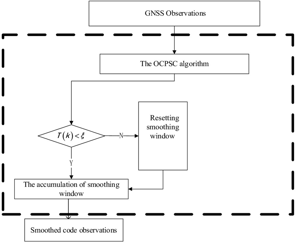
The processing steps of the OCPSC algorithm with the threshold detection for cycle slips (TDCS) are as follows (Fig. 1):
1.
Input GNSS observations.
2.
Use OCPSC algorithm to smooth GNSS code observations.
3.
Execute TDCS algorithm: while is less than the threshold for the cycle slip, the smoothing window width accumulates for positioning. Otherwise, the smoothing window is reset.
4.
Repeat Steps 1–3 to obtain the smoothed code observations for each satellite.
The Estimation of Ionospheric Slant Error
Since June 1998, the International GNSS Service (IGS) ionosphere working group has been maintaining the routine generation of the Global Ionospheric Maps (GIMs) (Li et al. 2019). GIM production is provided by the Center for Orbit Determination in Europe (CODE), which is an individual IGS analysis center. This paper applied the final GIM of the IGS, which is composed of GIM products. The Total Electron Content (TEC) message from the IGS final GIM is a grid data set in IONosphere map Exchange (IONEX) format (CDDIS 2021) with longitude ( resolution) and latitude ( resolution). GIMs provide the vertical delay at geographically defined ionospheric grid points (IGPs) (Park et al. 2017), which can be used to interpolate the ionospheric vertical error at an ionospheric pierce point (IPP).
When GNSS users obtain the ionospheric vertical error at the IPP, the ionospheric slant error can be obtained by the mapping function (Schaer 1999)where and = height of maximum electron density (450 km) on infinite thin spherical layer and approximate radius of Earth (6,378.1363 km), respectively; and = satellite elevation angle.
(16)
(17)
A Code Noise Estimation Method for Low-Cost Single-Frequency and Receivers
Because carrier-phase noise is much smaller than code noise, we assumed that carrier-phase noise can be neglected. Both the code noise and the carrier-phase noise obey a Gaussian distribution, in which the mean value is zero. According to Eq. (1), the code noise and multipath model can be expressed as the combination of dual-frequency (DF) measurements (Kee et al. 1997)where and = code noise and code observations, respectively, for-frequency ; = mean of ; and = carrier-phase observations for frequencies and , respectively; and = squared ratio of frequency to frequency .
(18)
(19)
These equations are not applicable to low-cost single-frequency receivers. In this study, we used ionospheric slant delay to calculate these values for single-frequency receivers [Eqs. (20) and (21)]. The ionospheric slant delay is estimated by using GIM and the ionospheric product provided by the IGSwhere = ionospheric slant delay estimated by using GIM.
(20)
(21)
Performance Analysis of the Optimal Carrier-Phase Smoothing Code
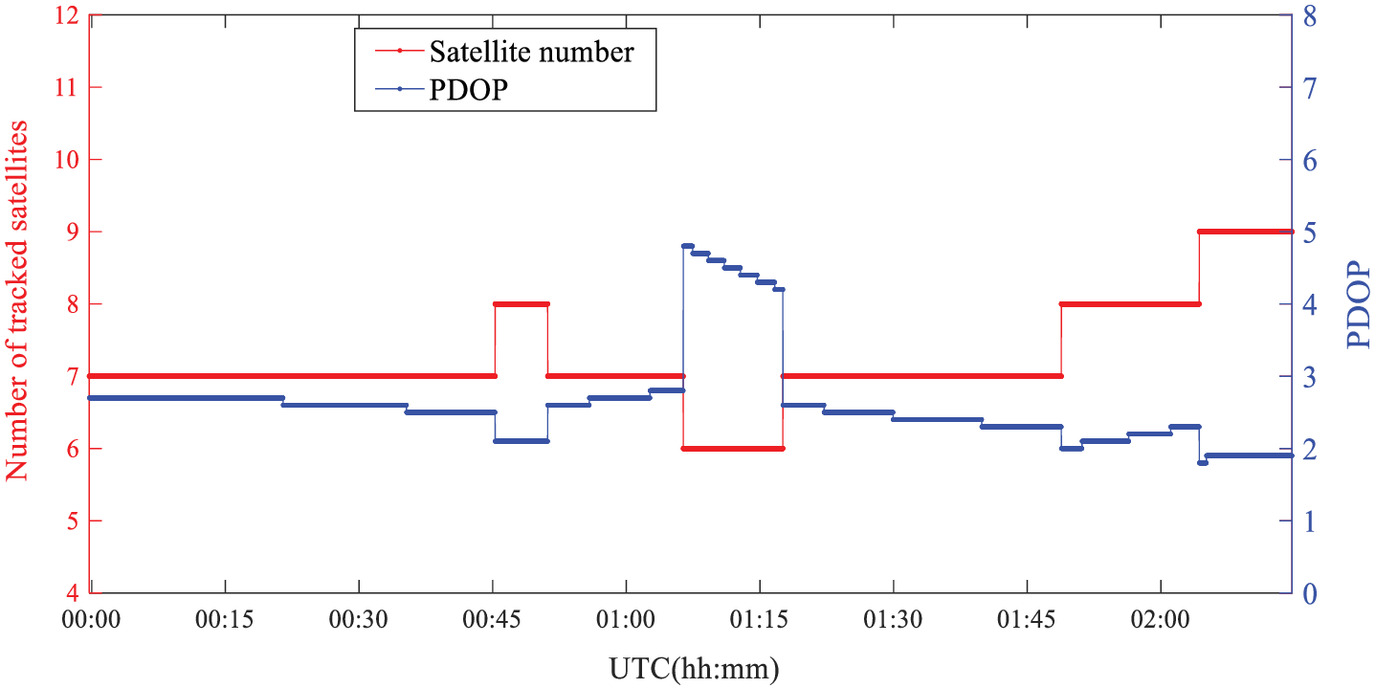
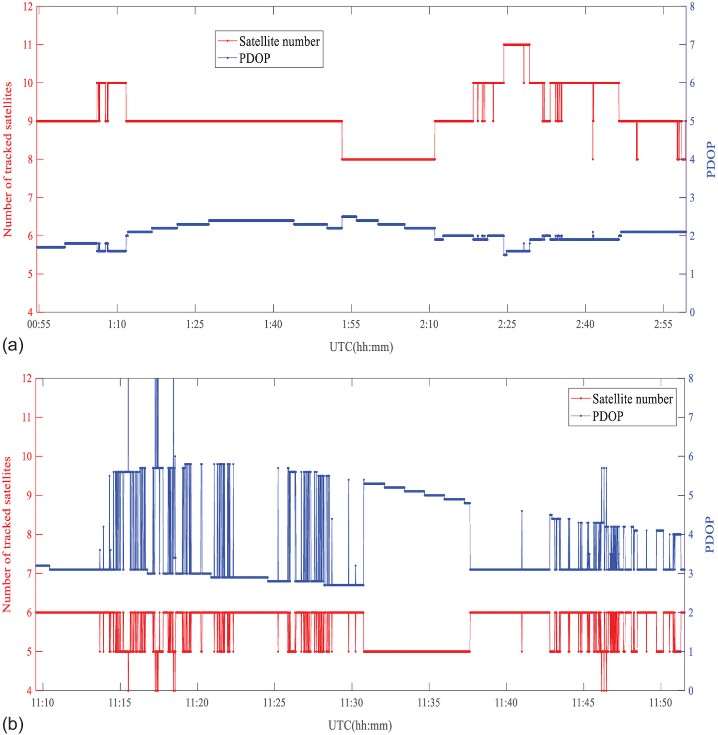
To verify the performance of the OCPSC, GNSS signals were received by a dual-frequency Trimble NetR9 receiver (Sunnyvale, California) at the JiuFeNG (JFNG) station. This receiver is a type of survey-grade receiver that is compatible with GPS, GLONASS, BeiDou, and Galileo constellations. Because GPS is a representative type of navigation system in GNSS, most researchers who study CPSC algorithms base their work on GPS observations. To verify the effectiveness of the OCPSC, this study used only GPS observations (Geng et al. 2019). GPS data from 00:00:00 to 2:15:00 on January 1, 2018 were collected and resampled at an interval of 1 s. The satellite elevation cutoff angle was set to 10°. Fig. 2 shows the period tracked by pseudorandom noise code (PRN) in the collected GPS data, and Fig. 3 shows the number of tracked satellites and the position dilution of precision (PDOP). There was a sudden decrease in the number of satellites between 0:44:16 and 1:17:42 Coordinated Universal Time (UTC) (Fig. 3). This was because GPS satellite G30 was not being tracked and G20 had not begun to be tracked during this time. Obviously, when the number of visible satellites increases, the PDOP value simultaneously decreases (Fig. 3).

Results of Cycle Slip Detection with Survey-Grade Receivers
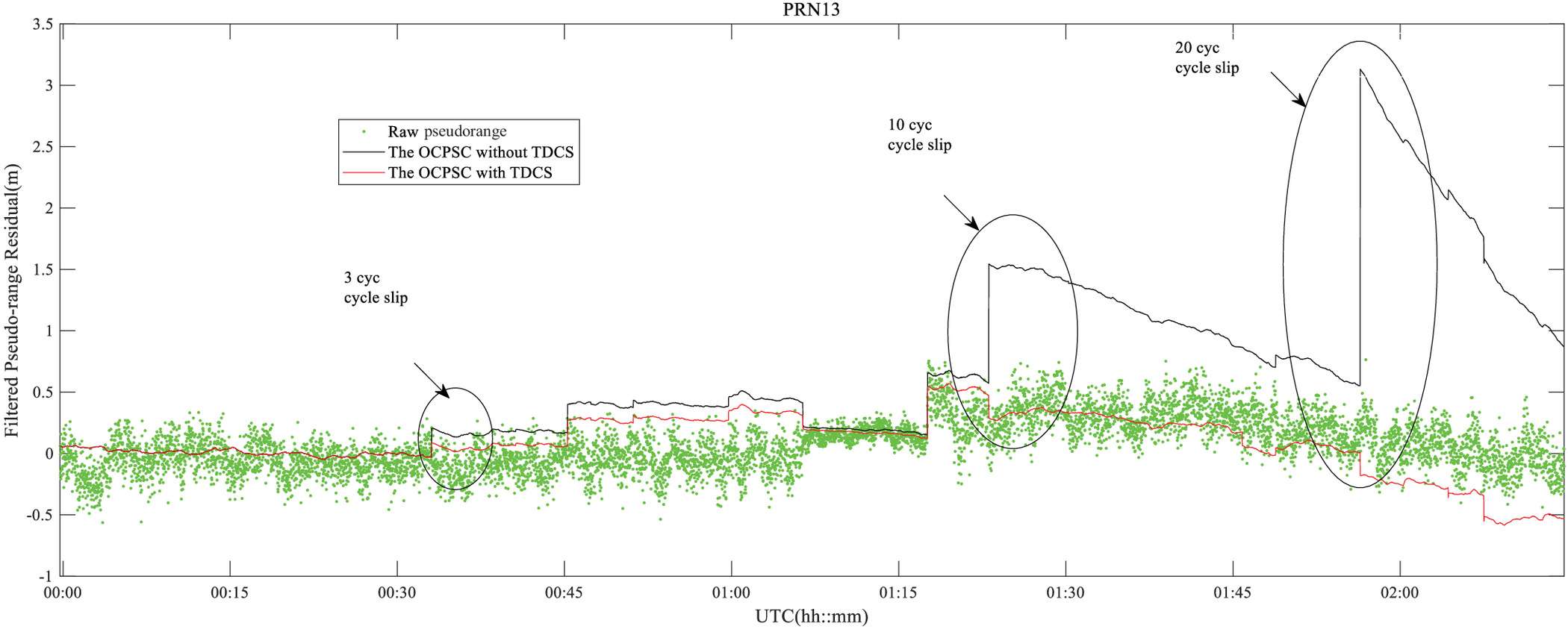
To verify the influence of the TDCS algorithm on suppressing the cycle slips, three instances of simulated cycle slips were added to the real measured GPS data. The ellipses in Fig. 4 indicate the 3 simulated cycle slip events, which included 3 cycles at UTC 00:33:01, 10 cycles at UTC 1:23:01, and 20 cycles at UTC 1:56:21. The OCPSC algorithm with TDCS and without TDCS effectively smoothed the pseudorange, and observation noise was reduced significantly (Fig. 4). However, when there are cycle slips in observations, a systematic bias, which is proportion to the magnitude of the cycle slips, will be introduced to the smoothed pseudorange until the smoothing window is reset (Chang et al. 2019). When a cycle slip of three cycles was added at UTC 00:33:01, the smoothed pseudorange residual was increased by about 0.5 m. When a cycle slip of 20 cycles was added at UTC 1:56:21, the smoothed pseudorange residual was increased by about 3.5 m. Unfortunately, the smoothed pseudorange residuals of the subsequent epochs will be affected until the smoothing window is reset. Therefore, it is necessary to integrate TDCS into the OCPSC algorithm to suppress the influence of cycle slips. Fortunately, our OCPSC algorithm with the TDCS can sensitively detect cycle slips at all epochs and automatically reset the smoothing window.
The Estimation of Variation of Ionospheric Error
Although CPSC performs well in noise reduction and is easy to implement, the variation of ionospheric error cannot be ignored. Dual-frequency (Kee et al. 1997) observations and single-frequency observations can be used to estimate the variation of ionosphere error between consecutive epochs [Eq. (10)]. The difference in ionosphere error between consecutive epochs can be calculated using Eqs. (22) and (23) for DF and SF observations, respectively
(22)
(23)
The performance of the traditional CPSC depends on the standard deviation of code noise and the variation of ionosphere error between consecutive epochs [Eq. (11)]. A small smoothing window is sensitive to the variation of ionosphere errors, but does not reduce noise sufficiently [Eq. (11)]. In contrast, a larger smoothing window is more effective in reducing noise, but cannot suppress the variation of ionosphere error, and may even lead to a divergence of the traditional CPSC. Therefore, the selection of smoothing window width is a kind of trade-off problem. Furthermore, we used dual-frequency observations from the JFNG site to analyze the variation of ionosphere error between consecutive epochs.
Fig. 5 shows the estimation of the variation of ionospheric error using the dual-frequency carrier phase and GIM for Satellite PRN02. The variation of ionospheric error calculated by GIM agreed well with average values calculated by the dual-frequency phase at all epochs, which verifies that the GIM performs well in estimating ionospheric error for single-frequency receivers (Fig. 5). Because the variation of ionospheric errors estimated using dual-frequency observations includes carrier-phase noise [Eq. (19)], it is much larger than the variation of ionospheric errors estimated using single-frequency observations
(24)

Code Noise Statistic for Single-Frequency Receivers
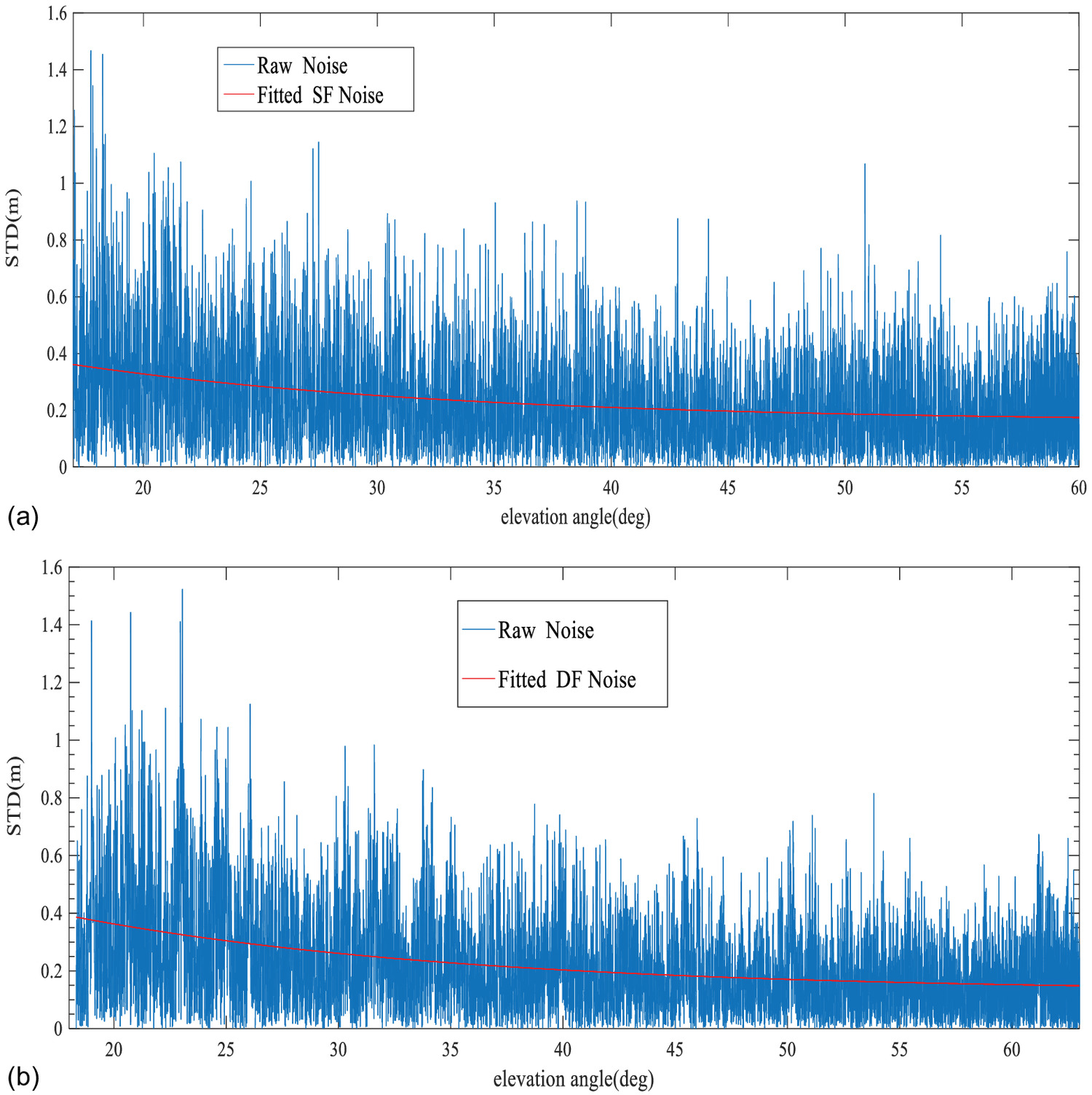
The measurement noise depends on the elevation angle and observation environment of the receiver antenna (Kee et al. 1997). We modeled the receivers’ code noise effects with the elevation angle () as follows:
(25)
To estimate the parameters , the standard deviation of the noise from dual-frequency observations and single-frequency observations were curve-fitted. When using and for curve fitting, is the mean value including the noise standard deviation of all observed satellites at the elevation angle. The parameters are listed in Table 1. There was almost no significant difference between the noise parameters of the dual-frequency observations and the single-frequency observations (Table 1). When the elevation angle decreased from 65° to 15°, the standard deviations of the observed noise for the single-frequency observations and the dual-frequency observations varied from 0 to 1.6 m, and the fitted standard deviations of noise varied from 0.2 to 0.4 m (Fig. 6). The results indicate that the fitting performance was the same for both the dual-frequency and the single-frequency observations.
| Frequency | Parameter | |||
|---|---|---|---|---|
| STD (m) | ||||
| DF | 0.0129 | 0.746 | 17.304 | 0.027 |
| SF | 0.164 | 0.789 | 15.013 | 0.031 |
The Optimal Smoothing Window Width for Carrier-Phase Smoothing Code
In the proposed OCPSC algorithm, the adaptive smoothing window width can be determined using the standard deviation of the code noise and the variation of ionospheric error between consecutive epochs [Eq. (11)]. The standard deviation of the code noise depends on the elevation angle in Eq. (25), and the variation of ionospheric error between consecutive epochs is estimated using the GIM in Eqs. (16) and (17).
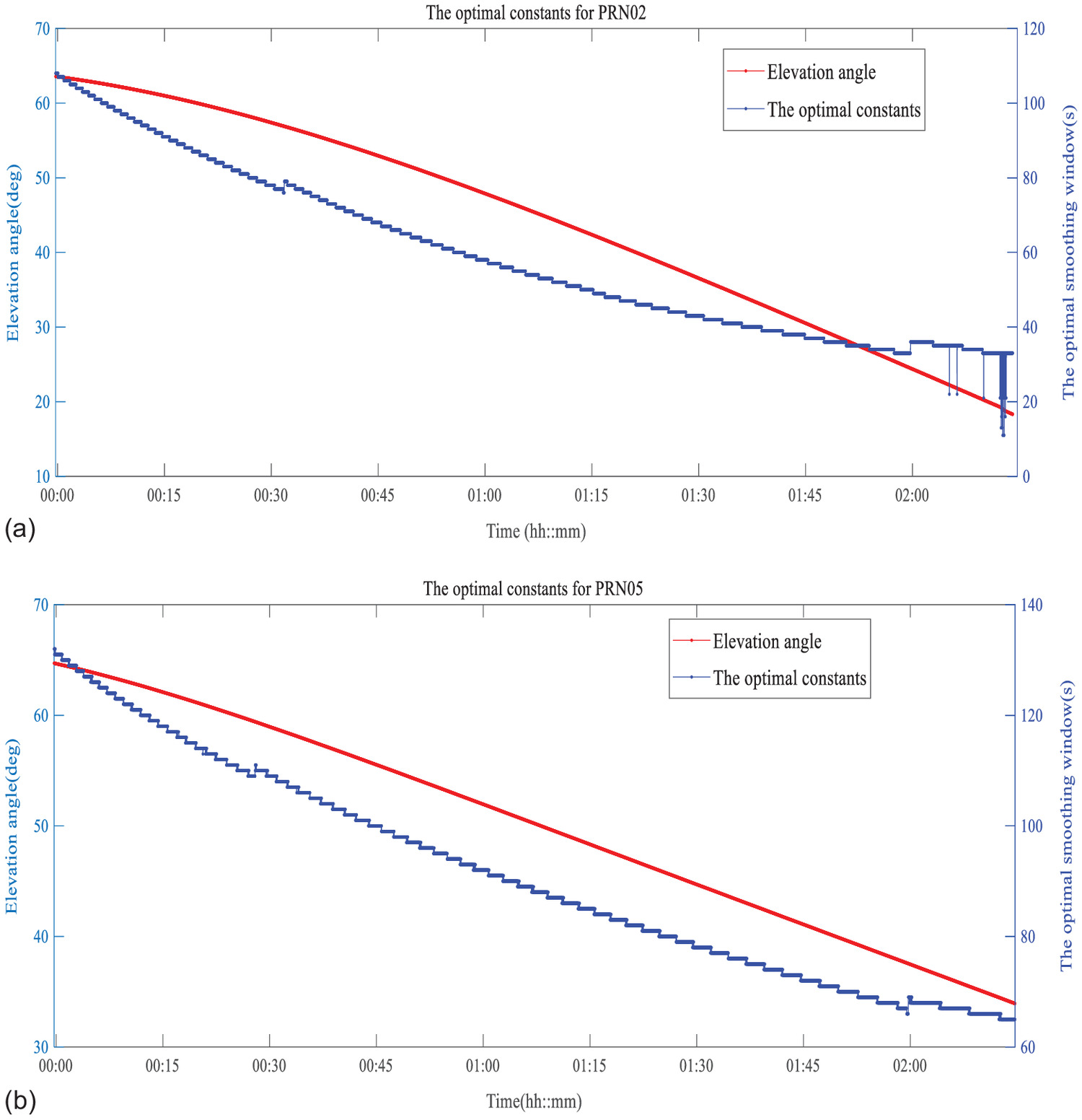
To prove that the optimal smoothing window width is flexible for each satellite and each epoch, we analyzed the relationship between the optimal smoothing window width and elevation angles of Satellites PRN02 and PRN05 (Fig. 7). The optimal smoothing window width varied from 110 to 15 s as the elevation angle varied from 65° to 15° for Satellite PRN02, which was similar to that for Satellite PRN05, but the optimal smoothing window width of Satellites PRN02 and PRN05 was different at the same epoch. In the Wullschleger et al. (2000), in the case of traditional CPSC, a smoothing window width greater than 100 s will reduce the noise level but simultaneously cause a large divergence error (Park et al. 2008). On the other hand, for some satellites at some epochs, when the smoothing window is as large as 1,000 s, the OCPSC algorithm can reduce the code noise without a serious divergence error.
Positioning Performance Analysis of the OCPSC Algorithm for Dual-Frequency Receiver
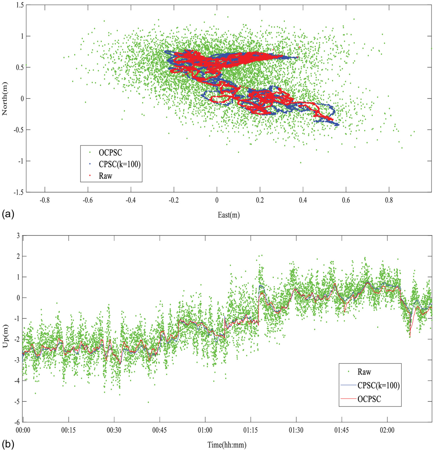
The dual-frequency observations were used to verify the OCPSC algorithm, and the true coordinates in the sinex file of the IGS product were used as reference values to assess the positioning performance of the raw code and the CPSC and OCPSC algorithms. In previous studies, the researchers proposed a fixed smoothing window of 100 s to obtain the best performance of traditional CPSC (Park et al. 2017). Therefore, the results derived using a fixed smoothing window of 100 s were used as a reference. A small cycle slip occurred in Satellite PRN13 at about UTC 00:44 (Fig. 4), which was not what we had simulated. This cycle slip had a serious impact on the performance of the traditional CPSC until the smoothing window was reset [Fig. 8(b)]. Our OCPSC algorithm can detect cycle slips in a timely and effective manner, and suppress the impact of cycle slips on positioning performance. Therefore, the OCPSC is more robust than traditional CPSC. Compared with the positioning accuracy of raw SPP, the horizontal positioning accuracy improved by about 0.04 m, and the vertical accuracy improved by about 0.1 m when applying the traditional CPSC with a smoothing window of 100 s (Fig. 8 and Table 2). The OCPSC algorithm with adaptive window width had better performance. It improved the horizontal accuracy and vertical accuracy by 0.05 and 0.3 m, respectively. Compared with the traditional CPSC, the positioning accuracy was not improved significantly by applying the OCPSC algorithm (Table 2). The horizontal positioning accuracy improved from 0.49 to only 0.48 m. This mainly was because the increase of the variation of ionospheric errors was not significant for traditional CPSC during the continuous observation period of about 2 h (Fig. 5).
| Method | JFNG | DAEJ | ||||
|---|---|---|---|---|---|---|
| Hor (m) | Ver (m) | Imp (hor, ver) (%) | Hor (m) | Ver (m) | Imp (hor, ver) (%) | |
| Raw code | 0.53 | 2.93 | 0, 0 | 0.76 | 1.50 | 0, 0 |
| CPSC () | 0.49 | 2.85 | 7.5, 2.7 | 0.75 | 1.44 | 2.3, 4.3 |
| OCPSC | 0.48 | 2.69 | 9.4, 8.2 | 0.67 | 1.38 | 12.6, 8.1 |
Note: Hor and Ver denote horizontal and vertical RMS, respectively; and Imp denotes Improvement rate compared with raw code.
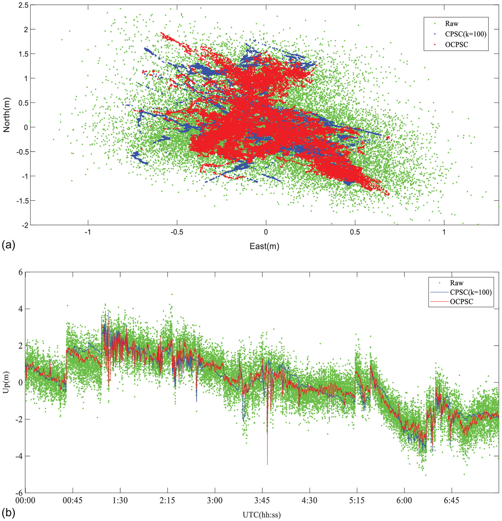
To illustrate more clearly that the OCPSC algorithm effectively can solve the problem between the reduction of noise and the increase of ionospheric error variation, a longer period of observation data were processed by the proposed algorithm. The DAEJeon (DAEJ) site data from GPS times 00:00:00 to 7:30:00 on March 1, 2022 were collected and resampled at an interval of 1 s. The positioning results of the DAEJ site are presented in Table 2 and Fig. 9. The CPSC with 100-s smoothing windows improved only 2.3% horizontally and 4.3% vertically compared with the raw SPP. Because the DAEJ site has longer observation times than Station JFNG, the increase of ionospheric error variation between consecutive epochs was larger for the DAEJ station than for the JFNG site. Therefore, when applying traditional CPSC with a smoothing window of 100 s, the improvement in horizontal positioning accuracy (2.3%) at the DAEJ site was smaller than that at the JFNG site (7.5%). Fortunately, the proposed OCPSC algorithm can reduce the ionospheric error variation between consecutive epochs that increases with the observation time. When applying the OCPSC, the improvement in horizontal positioning accuracy (12.6%) at the DAEJ site was larger than that at the JFNG site (9.4%).
Positioning Performance Analysis of the OCPSC Algorithm during Ionosphere Disturbances
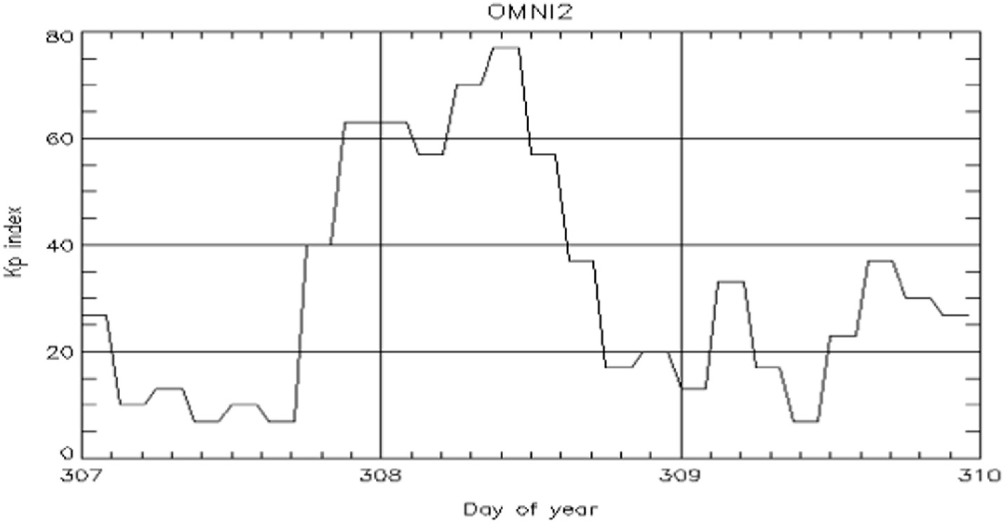
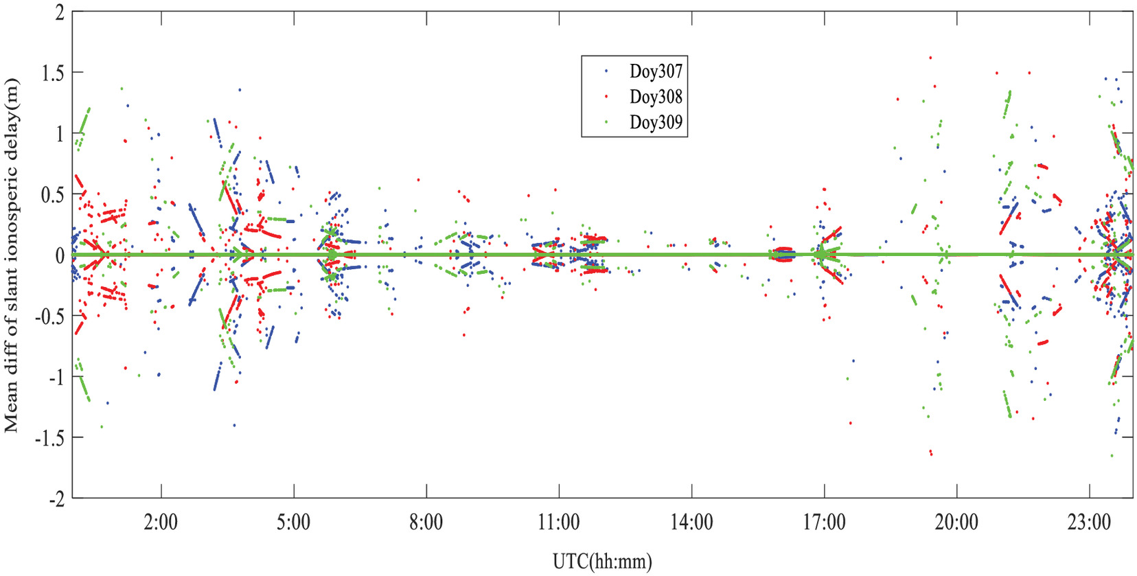
We investigated the positioning performance of the OCPSC during ionospheric storms. The 3-h-interval Kp-index can be used to measure global ionospheric disturbances (Bartels et al. 1939). The level of a geomagnetic storm is defined as Kp-index 5 for minor geomagnetic storms (G1), Kp-index 7 for moderate geomagnetic storms (G2), Kp-index 8 for stronger geomagnetic storms (G4), and Kp-index 9 for extreme geomagnetic storms (G5) (Hanslmeier 2002). The Kp-index is provided by NASA’s OMNIWeb Data Explorer (Papitashvili 2020). Fig. 10 shows the value of Kp-index from November 3 to 5, 2021. On November 4, 2021, there was an ionospheric storm between moderate and strong, with a Kp-index greater than 70.
To assess the positioning performance of the OCPSC algorithm during ionospheric storms, the algorithm was used to process observation data with high sampling intervals. The papeete (THTG) site data from GPS times 00:00:00 to 23:59:59 from November 3 to 5, 2021 were collected and resampled at an interval of 1 s. In this experiment, only frequency observation data were used. GIM estimated the mean variation of the ionospheric error for all visible satellites on November 3, 4, and 5, 2021 (Fig. 11). It is obvious that the variation of ionospheric error during the ionospheric storm (Fig. 11) was much higher than that in Fig. 5. Before 2:00 on November 4, 2011, more points deviated from zero in the variation of ionospheric error than on November 3 and 5, 2021, because the corresponding Kp-index was greater than that on the other two days. Between 8:00 and 17:00, with the decrease of the Kp-index, the variation of the ionospheric error also decreased and was closer to zero on November 3, 4, and 5, 2021. This illustrates that ionospheric storms significantly affect the variation of ionospheric errors.
The distribution of positioning errors in the horizontal and vertical directions during ionospheric storms is shown in Fig. 12 based on GPS data of the THTG station using the OCPSC algorithm. When many points in the variation of ionospheric error deviated from zero at UTC 5:27:52, the positioning error of the traditional CPSC increased by about 38 m, whereas the positioning error of the OCPSC was only about 10 m (Fig. 12). At UTC 19:35:50, when the variation of ionospheric error increased by 1.5 m, the residual of the traditional CPSC increased by about 15 m. the residual of the OCPSC increases by only about 10 m. Compared with the traditional CPSC, the OCPSC algorithm can suppress the influence of the variation of ionospheric error on positioning performance. Compared with raw SPP, the traditional CPSC did not improve the horizontal and vertical position accuracy, because the traditional CPSC does not consider the variation of the impact of ionospheric error on positioning performance (Fig. 12 and Table 3). However, compared with the raw SPP, the positioning errors of the OCPSC algorithm in the horizontal and vertical directions both were reduced by 0.01 m. Compared with the original SPP, the positioning accuracy of the OCPSC algorithm does not seem to be improved significantly. This mainly is because the OCPSC algorithm depends on the variation of ionospheric error to give an optimal window, which can constrain the impact of the variation of ionospheric error on positioning performance, rather than completely eliminating it.
| Method | Hor | Ver |
|---|---|---|
| Raw code | 3.24 | 2.92 |
| CPSC () | 3.26 | 3.10 |
| OCPSC | 3.23 | 2.91 |
Positioning Performance Analysis of the OCPSC Algorithm for Low-Cost Single-Frequency Receivers
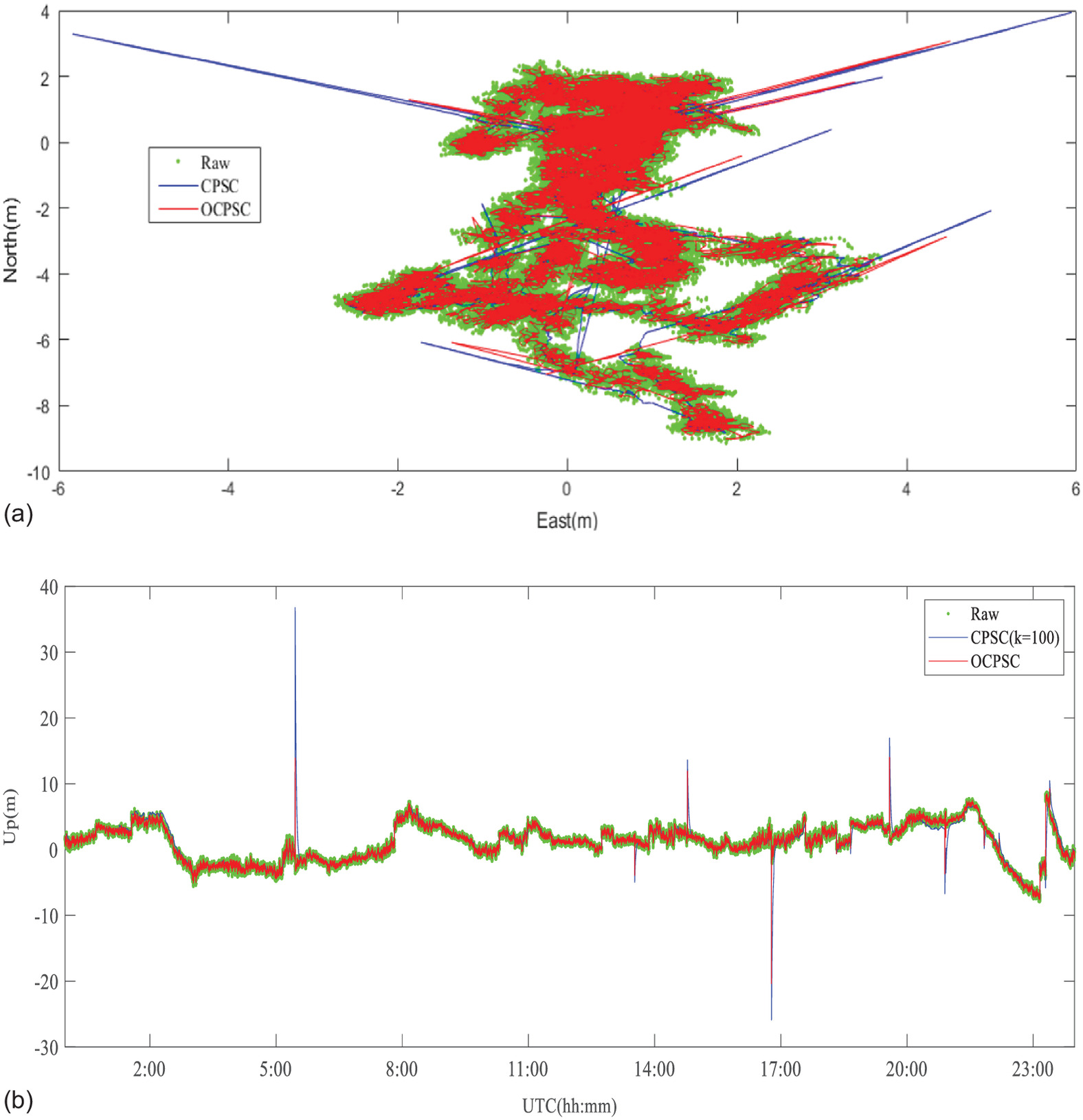
As mentioned previously, we conducted static experiments on dual-frequency and survey-grade receivers to verify that the OCPSC algorithm is effective. Then the OCPSC algorithm was applied to a u-blox EVK-M8T receiver (Thalwil, Switzerland), which is a low-cost single-frequency receiver. The u-blox receiver is an automotive-grade module that can track the signals from multiple GNSS constellations and provide raw pseudorange, carrier-phase, and Doppler observation (Odolinski et al. 2015). Because the u-blox receiver is connected to a patch antenna, it is applied widely to navigation, transport, traffic, and so forth. The positioning accuracy of low-cost single-frequency receivers for SPP usually is at the meter level (Pan et al. 2016), and at the decimeter level for real-time kinematics (Odolinski and Teunissen 2016). Therefore, in this paper, the RTK results were used for comparison to evaluate the positioning performance of the OCPSC algorithm with u-blox receivers.
To analyze the SPP positioning performance of low-cost single-frequency receivers using the OCPSC algorithm, static and kinematic experiments were carried out on Dengzhuang South Road, Haidian District, Beijing (Fig. 13). The observations from the u-blox receiver were recorded at a sampling interval of 1 s, and the satellite cutoff elevation angle was set to 10° to reduce the impact of obstacles. The static and kinematic data sets were collected on June 3, 2019 from local time 8:55:45 to 11:00:45, and on September 4, 2018 from local time 20:02:42 to 20:49:43. Fig. 14 shows the PDOP and satellite numbers of low-cost single-frequency receivers in static and kinematic experiments. In static experiments, the number of satellites was more than 7, and the PDOP was less than 3. In the kinematics experiment, which was affected by the obstacles in the observation environment, the number of satellites was between 4 and 6, and the PDOP was greater than 7.

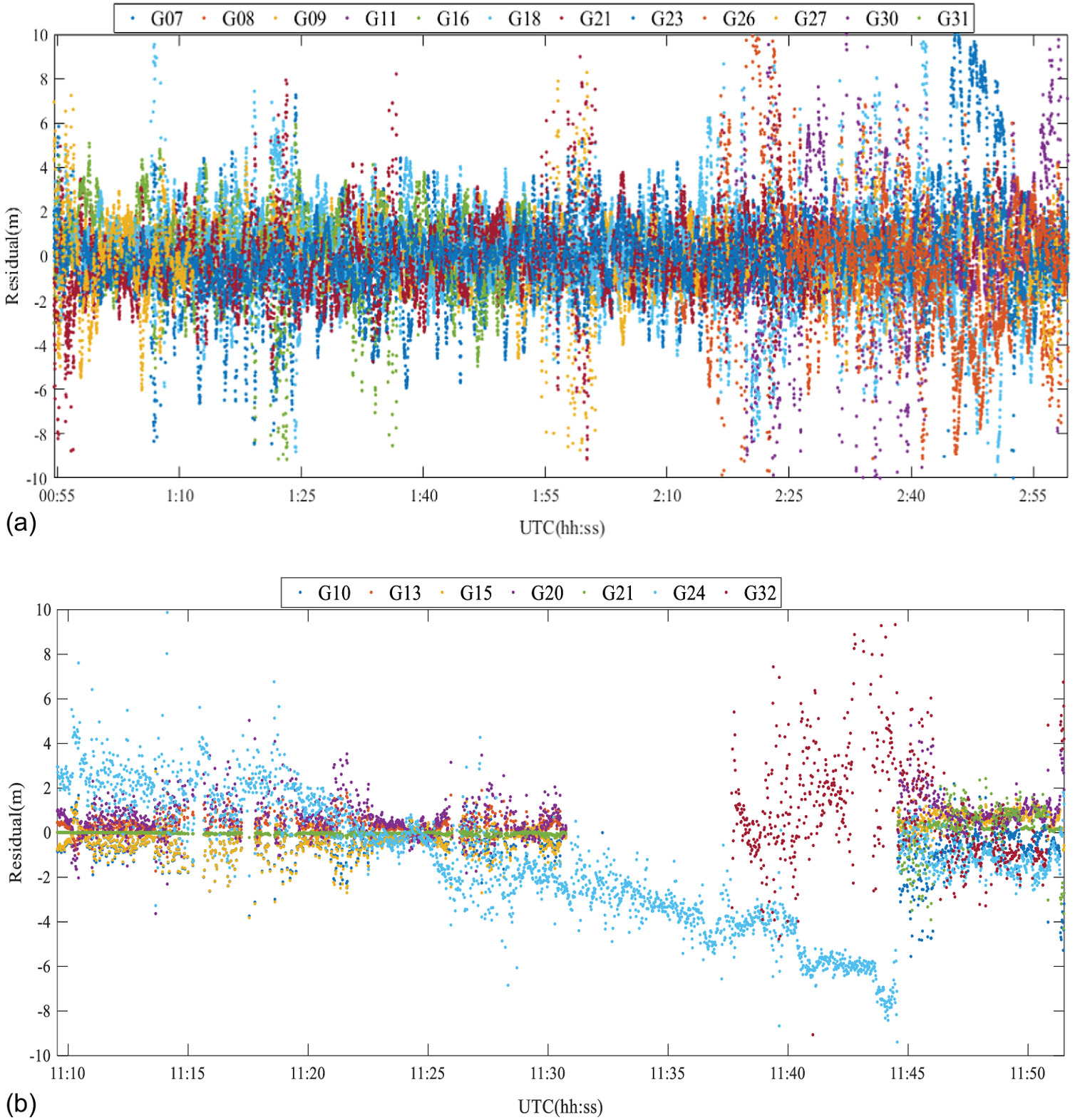
In the static test, the code observation residuals of each satellite fluctuated around zero [Fig. 15(a)]. However, in the kinematics test, because the observation was affected by the environment obstacles, the code observation residuals of many satellites had many multipath errors [Fig. 15(b)]. Both the traditional CPSC and the OCPSC algorithm can reduce the horizontal and vertical position errors (Figs. 16 and 17). In static testing, compared with the raw SPP, the horizontal and vertical errors of the traditional CPSC with a smoothing window of 100 s were reduced by 0.7 and 1 m, and the positioning accuracy improvement rates were 24% and 22.4%, respectively. This improvement in positioning accuracy is due mainly to the fact that low-cost single-frequency receivers include a great deal of noise when collecting data, whereas CPSC performs well in noise reduction. Compared with the traditional CPSC, the positioning error of the OCPSC algorithm was reduced by 0.15 and 0.21 m in the horizontal and vertical directions, respectively. The positioning accuracy improvement rate of the OCPSC algorithm was 28.9% and 27.4% compared with raw SPP. In the kinematics test, compared with the raw SPP, the positioning accuracy of the traditional CPSC improved by 0.02 m (0.5%) and 0.03 m (0.6%) (Table 4). Compared with the traditional CPSC, the positioning performance of the OCPSC algorithm was better, but the difference was not large. This mainly was because some observations, such as PRN24 and PRN32, may have a certain multipath error [Fig. 15(b)], resulting in little improvement in the positioning performance of the OCPSC algorithm.
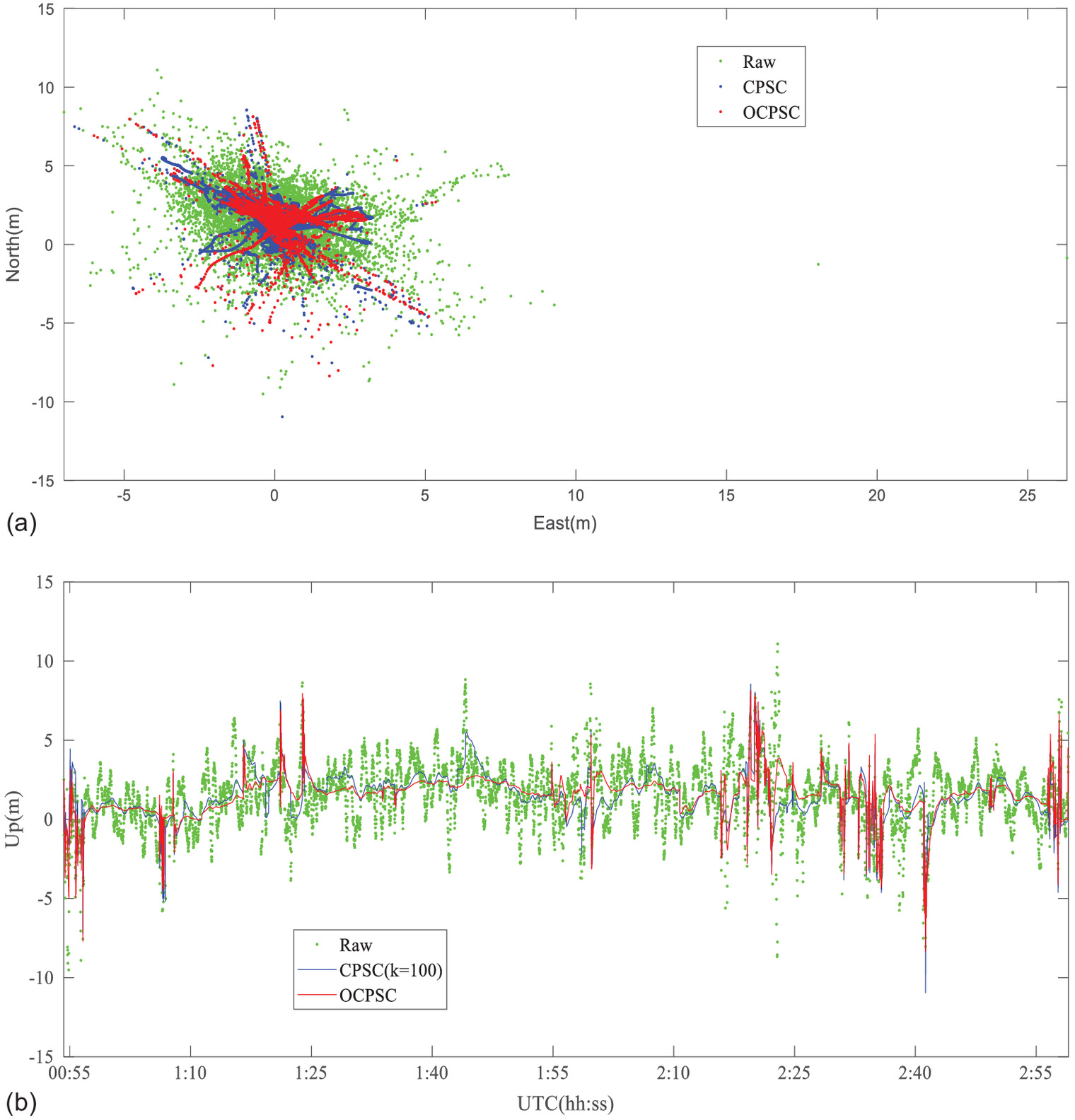
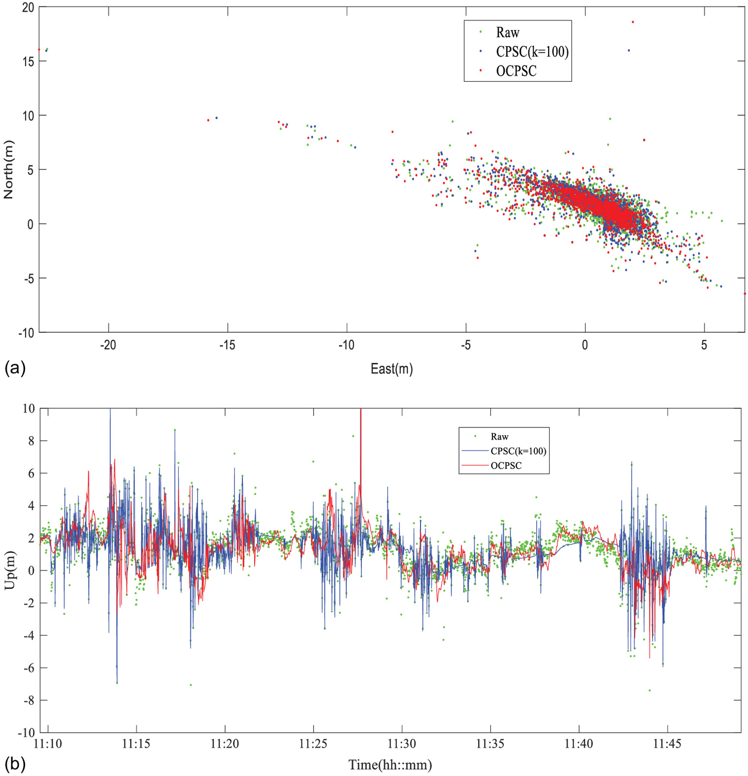
| Method | Static | Kinematic | ||||
|---|---|---|---|---|---|---|
| Hor (m) | Ver (m) | Per (hor, ver) (%) | Hor (m) | Ver (m) | Per (hor, ver) (%) | |
| Raw code | 3.08 | 4.24 | 0, 0 | 2.84 | 6.11 | 0, 0 |
| CPSC () | 2.34 | 3.29 | 24, 22.4 | 2.82 | 6.08 | 0.5, 0.6 |
| OCPSC | 2.19 | 3.08 | 28.9, 27.4 | 2.74 | 6.02 | 3.5, 1.5 |
Note: Hor and Ver denote horizontal and vertical RMS, respectively; and Imp denotes Improvement rate compared with raw code.
Conclusions
We analyzed the traditional CPSC method and its shortcomings. Subsequently, the cycle slip detection was introduced into traditional CPSC to mitigate the influence of the cycle slips. When the smoothing window moves forward, the variation of ionospheric errors will increase, and even may cause CPSC to diverge (Zhou and Li 2016). To solve this problem, GIM was used to estimate the variation of ionospheric error for low-cost single-frequency receivers. An estimation method is proposed for estimating noise and noise standard deviation. Furthermore, considering the estimated noise errors and the variation of ionospheric errors, we propose an OCPSC algorithm in which the smoothing window width varies adaptively for low-cost single-frequency receivers. Finally, verification experiments of dual-frequency receivers and application experiments of low-cost single-frequency receivers were carried out, and the following conclusions were drawn.
1.
The static verification experiment of dual-frequency receivers showed that compared with raw SPP, the horizontal and vertical positioning accuracies of the traditional CPSC improved about 0.04 m and 0.08 m in term of RMS, respectively. Compared with results derived using the traditional CPSC, positioning accuracies in the horizontal and vertical directions can be improved by 0.01 m (2%) and 0.16 m (6%), respectively when applying the OCPSC algorithm. Moreover, the OCPSC algorithm can detect cycle slips accurately and reset the smoothing window in time, thereby avoiding CPSC divergence due to a large cycle slip.
2.
In the static experiment with low-cost single-frequency receivers, when applying traditional CPSC, positioning accuracies in the horizontal and vertical directions are improved by 0.74 m (24%) and 0.95 m (22%), respectively. This difference with dual-frequency receivers may be due to the large noise of low-cost single-frequency receivers. Compared with the traditional CPSC, the OCPSC algorithm improved positioning accuracies in the horizontal and vertical directions by 0.15 m (6%) and 0.21 m (6%), respectively. These improvements were 0.08 m (3%) and 0.06 m (1%) in the kinematic experiment.
The proposed OCPSC algorithm has great potential to be applied widely to the future market of smartphone positioning, because future smartphones will integrate GNSS chips, and can be a dominant in the GNSS market. This algorithm improves positioning performance while maintaining the recursive and simple form of the traditional CPSC.
Data Availability Statement
Some data from low-cost single-frequency receivers, the OCPSC models, and the OCPSC code generated or used during the study are available from the corresponding author by reasonable request. The types of the raw data can be provided as a MAT file in MATLAB version R2018a.
Acknowledgments
Heartfelt thanks are given to the anonymous reviewers for their constructive comments to improve this manuscript and the experiment data using the u-blox receiver from Aerospace Information Research Institute (AIR), Chinese Academy of Sciences (CAS). This paper was supported by the National Natural Science Foundation of China (No. 11973073), the National Key Research and Development Program of China (No. 2016YFB0501405), the Basic Project of the Ministry of Science and Technology of China (No. 2015FY310200), and the Shanghai Key Laboratory of Space Navigation and Position Techniques (No. 06DZ22101).
Author contributions: X. Wang proposed the conceptualization for the study, supervised the progress of the study, provided advice on issues that arose, and performed writing—review and editing; X. Wang also was responsible for project administration and funding acquisition; H. Zhou established the study’s methods, analyzed the results, and wrote the manuscript; S. Li was responsible for validation, formal analysis, investigation, and writing—original draft preparation; and J. Fu, X. Chen, and J. Li provided suggestions for the model, and performed writing—review and editing. All authors have read and agreed to the published version of the manuscript.
References
Abdel-Hafez, M. F., Y. J. Lee, W. R. Williamson, J. D. Wolfe, and J. L. Speyer. 2003. “A high-integrity and efficient gps integer ambiguity resolution method.” Navigation 50 (4): 295–310. https://doi.org/10.1002/j.2161-4296.2003.tb00336.x.
Bahrami, M., and M. Ziebart. 2010. “Instantaneous Doppler-aided RTK positioning with single frequency receivers.” In Proc., Position Location & Navigation Symp, 70–78. New York: IEEE.
Bartels, J., N. H. Heck, and H. F. Johnston. 1939. “The three-hour-range index measuring geomagnetic activity.” J. Geophys. Res. 44 (4): 411. https://doi.org/10.1029/TE044i004p00411.
Cannon, M. E., K. P. Schwarz, and M. Wei. 1992. “A consistency test of airborne GPS using multiple monitor stations.” Bull. Grodrsique 66 (Mar): 2–11.
CDDIS. 2021. “GNSS data and product archive [online].” NASA’s Archive of Space Geodesy Data (CDDIS). Accessed October 1, 2020. https://omniweb.gsfc.nasa.gov/form/dx1.html.
Chang, G., T. Xu, C. Chen, B. Ji, and S. Li. 2019. “Switching position and range-domain carrier-smoothing-code filtering for GNSS positioning in harsh environments with intermittent satellite deficiencies.” J. Franklin Inst. 356 (9): 4928–4947.
Gao, Y., and K. Chen. 2004. “Performance analysis of precise point positioning using rea-time orbit and clock products.” Eng. Surv. Mapp. 3 (1&2): 95–100. https://doi.org/10.5081/jgps.3.1.95.
Geng, J., E. Jiang, G. Li, S. Xin, and N. Wei. 2019. “An improved Hatch filter algorithm towards sub-meter positioning using only Android raw GNSS measurements without external augmentation corrections.” Remote Sens. 11 (14): 1679–1699. https://doi.org/10.3390/rs11141679.
Hanslmeier, A. 2002. “The NOAA space weather scales.” In The sun and space weather, 193–200. Washington, DC: National Oceanic and Atmospheric Administration.
Hatch, R. 1982. “The synergism of GPS code and carrier measurements.” In Vol. 2 of Proc., 3rd Int. Geodetic Symp. on Satellite Doppler Positioning, 1213–1231. Las Cruces, NM: Physical Sciences Laboratory of New Mexico State Univ.
Kee, C., T. Walter, P. Enge, and B. Parkinson. 1997. “Quality control algorithms on WAAS wide-area reference stations.” Navigation 44 (1): 53–62. https://doi.org/10.1002/j.2161-4296.1997.tb01939.x.
Li, L., C. Jia, L. Zhao, J. Cheng, J. Liu, and J. Ding. 2016. “Real-time single frequency precise point positioning using SBAS corrections.” Sensors 16 (8): 1261–1274. https://doi.org/10.3390/s16081261.
Li, S., H. Zhou, J. Xu, Z. Wang, L. Li, and Y. Zheng. 2019. “Modeling and analysis of ionosphere TEC over China and adjacent areas based on EOF method.” Adv. Space Res. 64 (2): 400–414. https://doi.org/10.1016/j.asr.2019.04.018.
Odolinski, R., and P. J. G. Teunissen. 2016. “Single-frequency, dual-GNSS versus dual-frequency, single-GNSS: A low-cost and high-grade receivers GPS-BDS RTK analysis.” J. Geod. 90 (11): 1255–1278. https://doi.org/10.1007/s00190-016-0921-x.
Odolinski, R., P. J. G. Teunissen, and D. Odijk. 2015. “Combined BDS, Galileo, QZSS and GPS single-frequency RTK.” GPS Solutions 19 (Jan): 151–163. https://doi.org/10.1007/s10291-014-0376-6.
Pan, L., C. Cai, R. Santerre, and X. Zhang. 2016. “Performance evaluation of single-frequency point positioning with GPS, GLONASS, BeiDou and Galileo.” Surv. Rev. 49 (354): 197–205. https://doi.org/10.1080/00396265.2016.1151628.
Papitashvili, N. 2020. “OMNIWeb data explorer.” Accessed January 1, 2023. https://omniweb.gsfc.nasa.gov/form/dx1.html.
Park, B., C. Lim, Y. Yun, E. Kim, and C. Kee. 2017. “Optimal divergence-free Hatch filter for GNSS single-frequency measurement.” Sensors 17 (3): 448–468. https://doi.org/10.3390/s17030448.
Park, B., K. Sohn, and C. Kee. 2008. “Optimal Hatch filter with an adaptive smoothing window width.” J. Navig. 61 (3): 435–454. https://doi.org/10.1017/S0373463308004694.
Paziewski, J. 2021. “Multi-constellation single-frequency ionospheric-free precise point positioning with low-cost receivers.” GPS Solutions 26 (1): 23.
Schaer, S. 1999. Mapping and predicting the earth’s ionosphere using the global positioning system. Zürich, Switzerland: Schweizerische Geodätische Kommission.
Spoelstra, T. A. T., and H. Kelder. 1984. “Effects produced by the ionosphere on radio interferometry.” Radio Sci. 19 (3): 779–788.
Verhagen, S., D. Odijk, P. J. G. Teunissen, and L. Huisman. 2010. “Performance improvement with low-cost multi-GNSS receivers.” In Proc., 5th ESA Workshop on Satellite Navigation Technologies. New York: IEEE.
Wullschleger, V., R. Braff, and T. Urda. 2000. “FAA LAAS specification: Requirements for performance type.” In Proc., European Institutes of Navigation GNSS 2000 Conf. Stanford, CA: Stanford Univ.
Zhang, X., and P. Huang. 2014. “Optimal Hatch filter with an adaptive smoothing time based on SBAS.” In Vol. 31 of Proc., Int. Conf. on Soft Computing in Information Communication Technology, 34–38. New York: Springer.
Zhou, H., Z. Li, C. Liu, J. Xu, S. Li, and K. Zhou. 2020. “Assessment of the performance of carrier-phase and Doppler smoothing code for low-cost GNSS receiver positioning.” Results Phys. 19 (Dec): 103574.
Zhou, Z., and B. Li. 2016. “Optimal Doppler-aided smoothing strategy for GNSS navigation.” GPS Solutions 21: 197–210.
Information & Authors
Information
Published In

Journal of Surveying Engineering
Volume 149 • Issue 4 • November 2023
Copyright
This work is made available under the terms of the Creative Commons Attribution 4.0 International license, https://creativecommons.org/licenses/by/4.0/.
History
Received: Sep 10, 2022
Accepted: Apr 13, 2023
Published online: Jun 27, 2023
Published in print: Nov 1, 2023
Discussion open until: Nov 27, 2023
ASCE Technical Topics:
- Algorithms
- Benefit cost ratios
- Business management
- Construction engineering
- Construction management
- Engineering fundamentals
- Environmental engineering
- Errors (statistics)
- Financial management
- Geomatics
- Global navigation satellite systems
- Grid systems
- Mathematics
- Noise pollution
- Pollution
- Practice and Profession
- Standards and codes
- Statistics
- Structural engineering
- Structural systems
- Surveying methods
- Systems engineering
- Systems management
- Windows
Authors
Metrics & Citations
Metrics
Citations
Download citation
If you have the appropriate software installed, you can download article citation data to the citation manager of your choice. Simply select your manager software from the list below and click Download.