Abstract
One of the goals of infrastructure asset management research is to find appropriate repair policies for infrastructure systems. The annual repair cost of the system may vary when a repair policy meant only to minimize life cycle cost is applied to each facility in the system. Such variance in the annual repair cost leads to difficulty in securing the budget for system managers; thus, a desirable, practicable repair policy should reduce not only life cycle cost but also the dispersion of annual repair cost. In this study, we first formulate a network-level repair policy optimization problem for an infrastructure system comprising a finite number of facilities to minimize the total cost over the planning period, which is defined as the weighted sum of the repair cost and its variance. Then we propose two methods for solving it: (1) the exact one based on the Markov decision process; and (2) an approximate one using preventive repair rules. The former can be used in small-scale systems, whereas the latter can be used to simplify the repair policy regardless of the size of the system and to determine an approximate repair policy for large-scale systems. The proposed methodology is applied to two numerical investigations of (1) a small-scale infrastructure system; and (2) a large-scale infrastructure system. In the first case, we find the Pareto frontier of the repair cost and the variance in annual repair costs by the exact solution method and show that the preventive repair rule–based method provides a near-optimal solution. In the other case, the preventive repair rule–based method leads to a superior policy on aggregation of the optimal solutions independently found for each decomposed subsystem.
Introduction
Issue and Concept
In the field of infrastructure asset management, various methodologies based on mathematical models, optimization methods, and simulations have been developed for minimizing the expected life cycle cost of infrastructure systems that consist of multiple infrastructure facilities. When considering the repair policy for infrastructure systems comprising multiple infrastructure facilities, even if the expected annual repair cost does not change over the years, the uncertainty of the deterioration process causes variations in the timing of repair for each facility, and the actual annual repair cost of the system varies because of the finiteness of the number of the facilities in the system.
Here we study asset management systems that adopt the single-year budget principle, where the annual budget for repair work is usually fixed. When the optimal repair policy focusing only on minimizing the expected life cycle cost is applied, the actual repair cost may significantly differ from the given budget, and the possibly excessive difference between these amounts might hinder securing the budget and even lead to inefficient use of the latter. In a chain reaction, this might lead to underestimation of the next-year budget and consequently to an increased risk of deterioration because an underestimated budget might be insufficient for the necessary repair. Additionally, variation in the quantity of repair work not only affects the business conditions of the contractors by generating difficulties in securing order opportunities but also leads to difficulty in securing resources for repair work, including construction machines and material. Hence, a practicable, desirable repair policy should consider not only minimization of the life cycle cost but also leveling of the annual repair cost.
An intuitive concept of this study is represented in Fig. 1. However, although the figure illustrates deterministic deterioration processes, the proposed methodology assumes stochastic deterioration processes. In addition, we assume homogeneous stochastic deterioration processes (i.e., the same Markov transition probabilities) for each facility, but the deterioration processes realized according to the stochastic process can be heterogeneous as illustrated in the figure. In the figure, we consider an infrastructure system comprising two facilities and show the variation in the total cost of repairing them. It is assumed here that two repair methods are available as shown in the figure: corrective repair and preventive repair. The deterioration and repair process for each facility is represented by the time evolution of the condition state (CS). The graphs in the left column assume a situation where a repair policy that only considers minimizing the total repair cost (life cycle cost) is adopted. Here we suppose that a repair policy that executes only corrective repairs—the corrective repair policy—minimizes the life cycle cost. In this situation, the annual repair cost may vary over years, as shown in the bottom graph. The graphs in the right column assume a situation where a repair policy that considers cost leveling is adopted. In this situation, as shown in the bottom graph, by advancing the repairs to Facility 2, the variance in the annual repair cost is reduced; that is, cost leveling is achieved, although the life cycle cost is slightly increased. For cost leveling, the decision on whether or not to advance the repair of Facility 2 should be made by also considering the CS of Facility 1. This means that optimal repair policies for each facility are not guaranteed to be optimal for the system. Thus, the problem of optimizing the repair policy considering cost leveling becomes a network-level problem that determines the facility to be repaired according to the combination of the CSs of the individual facilities in the system. Additionally, advancing the repair of Facility 2 for cost leveling can be interpreted as executing preventive repair. Thus, it is likely that cost leveling can be attained through the effective execution of preventive repairs. Note that Fig. 1 assumes that preventive repairs for cost leveling are additionally executed in addition to the corrective repair policy, but in situations where preventive repairs are basically executed (e.g., a situation where a repair policy that includes the execution of preventive repairs minimizes the life cycle cost), cost leveling might be achieved by partially suppressing the execution of preventive repairs. It is presumed that the approximate solution method proposed in this study can be applied to such situations because it can also provide a solution that suppresses preventive repairs.

Research Objectives and Structure
Although more details will be described in the literature review section, the following issues remain unresolved in state-of-the-art research on cost leveling: (1) there is no model to derive the optimal repair policy at the network level by considering by using a stochastic model to consider the uncertainty of the deterioration process of each facility in the system; and (2) there is no method to derive an optimal or approximate solution to the network-level cost-leveling problem with stochastic deterioration processes while eliminating combinatorial explosion. To bridge the gap, we set the objectives of this study as follows:
•
Formulate a network-level repair policy optimization problem for infrastructure systems consisting of finitely many facilities, considering both cost minimization and cost leveling, in situations where the future deterioration process involves uncertainty.
•
Propose two methods for solving the formulated optimization problem: (1) an exact solution method based on dynamic programming for small-scale systems; and (2) an approximate solution method using preventive repair rules to simplify the repair policy regardless of the size of the system and to determine an approximate repair policy for large-scale systems.
•
Verify the effectiveness of the proposed methodology through numerical examples by discussing the properties of solutions and evaluating the accuracy of approximation methods.
The remainder of this paper is organized into the following sections. In “Literature Review,” we review previous studies from two perspectives: optimization models and solution methods. In “Problem Formulation,” we formulate an optimal repair policy problem considering life cycle cost minimization and annual cost leveling. In “Determination of Repair Policy,” we propose the two solution methods. In “Numerical Study,” we present numerical studies of a small-scale system to compare the two solution methods and a large-scale system to investigate the performance of the proposed approximation method. In “Summary and Future Tasks,” we provide conclusions and future research directions. A list of notations is given at the end of this paper and can be referred to in reading the “Problem Formulation” and “Determination of Repair Policy” sections.
Literature Review
Models
Here we review some mathematical optimization models for providing repair policies (also called management policies, maintenance policies, intervention policies, etc.) for infrastructure systems, focusing on the properties of their objective functions. They can be classified into project-level (also called object-level or facility-level) and network-level (also called system-level) models. In project-level models, the total repair cost or total social surplus is set as the objective function for a single facility (Friesz and Fernandez 1979; Madanat 1993; Madanat and Ben-Akiva 1994; Li and Madanat 2002; Brühwiler and Adey 2005; Ouyang and Madanat 2006; Jido et al. 2008). In network-level models, interdependencies among objects (facilities) are considered. For example, models have been proposed that consider the budget constraints of the entire system (Kuhn and Madanat 2005; Sathaye and Madanat 2011; Lee and Madanat 2015); resource constraints (human resources, equipment, etc.) for the entire system (Fwa et al. 1994; Chu and Huang 2018); user costs due to deterioration and repair works (Ouyang and Madanat 2004; Durango-Cohen and Sarutipand 2007; Ouyang 2007; Medury and Madanat 2013; Hu et al. 2015); and economies of scale by repair synchronization (Mizutani et al. 2020). Among them, many models represent the uncertainty of a deterioration process as stochastic.
As described in the “Introduction,” repair policy optimization models that consider cost leveling are network-level models that account for the interdependence among facilities. The models presented in previous studies on cost leveling can also be generally classified as network-level. Previous studies considering cost leveling have focused on the short-term (several years) construction-sequencing problem (i.e., determining the timing of each work process in a series of short-term construction works) rather than on long-term repair policy optimization problems. Such short-term problems originated with studies of the resource-leveling problem (Woodworth and Willie 1975; Easa 1989; Harris 1990) and have subsequently evolved into weighted total minimization problems of a cost and its variance (Takamoto et al. 1995; Savin et al. 1997), and with studies on achieving cost leveling by the minimum moment method (Kartam and Tongthong 1998; Leu et al. 2000; Hiyassat 2001; Christodoulou et al. 2010). In Yoon et al. (2014), cost leveling in maintenance and asset management were targeted; however, the considered planning period was short (three years), making it difficult to derive long-term repair policies. The deterioration of infrastructure is a long-term process, and the effects of advancements in repair, as shown in Fig. 1, remain relevant for a long time. Thus, to properly consider cost leveling, it is desirable to use a model that determines repair policies in a long-term framework. Additionally, in the aforementioned studies, the deterioration process was assumed to be deterministic. Although the models recalled were network-level, there were a few project-level models that were exceptionally similar to the concept of cost leveling. Yoon et al. (2017) proposed a model to find a long-term repair policy with cost leveling of a single facility assuming a deterministic deterioration process. The contribution of Boyles et al. (2010) can be interpreted as proposing a model similar to the one in this study in the sense that it considered nonlinear preferences for repair costs in a project-level model. However, since it was a project-level model, it would be unable to achieve the objectives of the present study.
The aforementioned studies, as well as this study, attempted to achieve cost leveling directly (an indicator of the variance in repair costs is explicitly included in the objective function). On the other hand, studies that consider the budget constraint for the entire network can consequently demonstrate a cost-leveling effect, even though they do not directly aim at cost leveling. Many studies have been performed to derive network-level optimal repair policies that satisfy the budget constraint assuming a deterministic deterioration process (Lee and Madanat 2015; France-Mensah et al. 2019; Kothari et al. 2022). However, when budget constraints are considered in a stochastic deterioration process, a feasible solution to satisfy the budget constraint does not exist, unless conditions are set so that the occurrence probability of the situations that do not satisfy the budget constraint is zero. Studies on long-term (a sufficiently long finite time horizon, such as decades, or an infinite time horizon) repair policy optimization considering budget constraints for stochastic deterioration processes set restrictions on the analytical framework, such as (1) budget constraints only on the expected values with respect to possible condition states (there is a possibility of budget overruns in reality) (Smilowitz and Madanat 2000); and (2) constraints on the stochastic deterioration process (e.g., assuming that no sudden and unexpected deterioration occurs and that only transitions to adjacent condition states occur) (Kuhn and Madanat 2005; Sathaye and Madanat 2011; Guo et al. 2020). To avoid such restrictions, it is necessary to consider cost leveling directly in a stochastic deterioration process, rather than attempting to indirectly achieve the cost-leveling effect by establishing a budget constraint. However, to the best of the authors’ knowledge, no network-level optimization model has ever been proposed to obtain a long-term repair policy considering the cost-leveling effect directly under the assumption of a stochastic deterioration process.
Solution Method
We review some solution methods for network-level models used for deriving long-term repair policies considering stochastic deterioration processes. As the previous models for cost-leveling consider a deterministic deterioration process, it would be significantly inaccurate to adopt their solution methods for dealing with the Markov decision process used in this study. For small-scale systems, an exact solution of the optimal repair policy at the network level can be found even if the deterioration process is stochastic (Mizutani et al. 2020). Conversely, in realistic-scale systems, because of the combinatorial explosions of both the possible states and the solution space, the problem of deriving optimal repair policies at the network level often leads to difficulties in deriving the exact solution.
Motivated by this, solution methods that approximate the objective function using machine learning (Medury and Madanat 2013; Li et al. 2014; Carvalho et al. 2019) or meta-heuristic methods such as genetic algorithms, simulated annealing, or ant colony optimization (Chan et al. 1994; Fwa et al. 1994; Lee and Madanat 2015; Kielhauser et al. 2017; Zhang et al. 2017) are sometimes used. Nevertheless, generally the repair policies derived by these methods are in the form of specifying the facilities to be repaired for each of a huge number of states, and their applicability in practice is questionable.
Since cost leveling is considered in this study to provide a practical model, it would be desirable to provide the solution in a practical form as well. As previous studies may be able to meet such practical requirements, there are solution methods that reduce the dimensionality of the state and decision variables when approximating the objective function, as follows. Smilowitz and Madanat (2000) suggested a solution method that simplifies the problem by defining state variables for an infrastructure system consisting of homogeneous facilities such that the deterioration state of each facility is aggregated into the number of facilities per deterioration state. Mizutani et al. (2020) proposed an approximation method for finding repair and work zone policies by solution space reduction techniques that (1) use a simplified rule to determine a huge number of decision variables that specify whether each facility in an infrastructure system needs to be repaired or work-zoned; and (2) optimize only a few of the operational variables in the rule. In the present study, we employ some ideas from the latter two sources to develop a solution method for the proposed model that considers cost leveling. Note that, according to the classification by Sathaye and Madanat (2011), the proposed solution method is classified as a top-down approach, which is for homogeneous facilities. Although it is conceivable to use a bottom-up approach that can consider heterogeneous facilities, we design the solution method in this study with emphasis on proposing a calculable solution method. Nevertheless, to the best of the authors’ knowledge, a solution method identical to the preventive repair rule–based policy proposed in this study has not been proposed in the literature. Additionally, it seems that the effect of preventive repairs on cost reduction has been the focus of conventional analysis, and there have been no studies discussing the effect and implementation of preventive repairs from the perspective of cost leveling as performed in this study.
Problem Formulation
Discrete Time Axis
We define a discrete time axis as consisting of time points that extends to infinite with a fixed interval ; that is, , . We denote the infinite set of inspection time points by . At each time point , an inspection of the entire system is conducted and the CS of each facility in the system is observed. The system manager has to decide which facilities to repair and what types of repair work to perform for the entire system according to the CS inspected.
State Vector
In this study, we target an infrastructure system comprising identical (homogeneous) facilities that have the same utility, deterioration process, and repair cost function. We assume the CS of a single facility to be represented by discrete ratings; the state space of the CS is defined as . When CS takes the value , it means that the facility is in the worst condition, whereas a CS value of 1 represents a facility in its best condition. Hence, the higher the CS, the more deteriorated the facility is. To simplify the expression for the condition of the entire system, information on the CS of each facility at time point is aggregated into a state vector representing the number of facilities per each CS. Specifically, the state vector of the system at time point is defined aswhere = number of facilities with CS at time point . To distinguish them before and after repair at time point , we use and to denote the state vectors before and after repair, respectively. The number of possible patterns for the state vector is . Without loss of generality, we assign an element identification number to each state vector, where is the state space of the identification number. The state space of the state vectors is denoted . Denote also by the number of facilities with CS corresponding to the state vector .
(1)
(2)
Deterioration Process
A deterioration process of a facility is modeled as a stochastic progression to be able to consider the uncertainty inherent in it. Assuming that each facility in the system is identical, the same Markov process can be adopted for each of them. The Markov transition probability of the change of CS from to between and is defined aswhere and = CSs at time point before and after repair, respectively. The Markov transition probability has following properties:
(3)
(4)
(5)
(6)
The Markov transition probability matrix of a single facility is then defined as follows:where = upper triangular matrix because of Eq. (5).
(7)
To calculate the transition probability of the state vector, we consider a state variation matrix that represents the amount of change in the number of facilities in each CS. When CS changes from to , a state variation matrix is defined aswhere = number of facilities whose CSs change from to when the state vector changes from to ; and th element of . The occurrence probability of a state variation matrix (i.e., the conditional occurrence probability of with given ) can be given, based on the multinomial distribution, as
(8)
(9)
(10)
(11)
Since there exist multiple patterns of the state variation matrix that satisfy Eqs. (9) and (10) for the same pair , we define the set of all possible state variation matrices as follows:
(12)
Now we can derive the transition probability of the state vector from to as the sum of the probabilities of all state variation matrices in ; that is
(13)
The transition probability has the following properties:
(14)
(15)
(16)
The deterioration process of the entire system is expressed as the transition probability matrix for state vectors
(17)
Repair Process
We assume that one type of repair method is available for each CS before repair, and is the CS after repair when a facility with CS is repaired. With slight modifications to the framework of this study, the selection of multiple repair methods for a CS before repair can also be considered; however, the preventive repair rule–based policy may become cumbersome. When the state vector at time point before repair is and repair policy is applied, the repair process can be formulated as the transition of the state vector from to at time point as follows (where we assume that the time for the determination and execution of the repair policy is relatively small, and hence can be ignored throughout this paper):
(18)
(19)
(20)
(21)
(22)
(23)
(24)
A transition probability of the Markov chain, can also be interpreted as the ratio (repair ratio) of to be repaired. We denote by the identification number of the possible repair policies, and is the set of possible repair policies. For example, if there are three possible repair policies , . Once is determined, the value of is uniquely selected from , where is the th element of . Then, once is determined, the correspondence of the transition from to is deterministically and uniquely specified. However, even if we define this transition correspondence, may not be uniquely determined. Additionally, since the size of the set of varies with the number of facilities , we denote with the subscript .
In Eq. (18), is the operator matrix that converts the state vector before the repair to that after the repair, and means the ratio of the number of facilities with CS before repair whose CSs become after repair to . Following the concept of “randomized policy” in Smilowitz and Madanat (2000), the ratio is treated as a decision variable, and the facilities to be repaired are not specified.
Although it is possible to set the operator matrix to be time-variant, to obtain a time-invariant steady-state solution, the repair CS transition matrix is assumed to be constant with respect to time; namely
(25)
Additionally, it is supposed that the facilities with the maximum CS at each time point must be repaired; that isand the facilities with CS 1 need not be repaired; that is
(26)
(27)
With the operator matrix , the repair process of the entire system with given is expressed as the deterministic transition matrix of the state vectors, so
(28)
(29)
Objective Function
We consider finding an optimal repair policy that considers both life cycle cost minimization and annual cost leveling. Specifically, we define the cost corresponding to each year as the expected value of the weighted sum of the annual repair cost and its variance and then find the optimal repair policy as the solution to the problem to minimize the total cost over years. The time evolution of the state of the system is modeled stochastically as a dynamic variation of the state vector, which aggregately represents the deterioration and repair processes of each facility. Note that the values of the elements of the deterioration transition probability matrix fluctuate between 0 and 1 because the deterioration process is a stochastic process, whereas the those of the repair transition matrix are 0 or 1 because the repair process is not a stochastic one.
Supposing the repair policy is given, the occurrence probability vector of the state vector before repair at each time point, , can be calculated using and aswhere = occurrence probability that the state vector before repair is at time point . When the time point is close to infinity (), the deterioration and repair process converges into a steady state and its occurrence probability vector satisfies the conditionwhere = occurrence probability of the state vector before repair in the steady state. Supposing the repair policy is and the state vector before repair is , the repair cost at that time point can be given aswhere = unit cost per facility to perform the repair that alters the CS from to .
(30)
(31)
(32)
(33)
(34)
Since the state vector is a random vector, the repair cost at each time point also varies stochastically. For a given repair policy , the expected value and variance of the annual repair cost at a time point in the steady state are given byrespectively. Based on Eqs. (35) and (36), the cost function to be minimized can be defined as the discounted present value of the sum of the expected values of the annual repair costs and their variances over an infinite horizon; namelywhere = expected value of the input with respect to the random vector ; = discount factor; and = relative weight between the annual repair cost and its variance. In this study, we interpret the variance as an additional switching cost (e.g., financing cost) caused by cost variation. In this case, can be interpreted as a weight to convert the variance into the monetary scale. In order to treat the variance as the switching cost, which is preferably discounted with respect to time, we formulate the objective function in Eq. (37) by explicitly considering the variance at each time point. Note that we use variance as the index of dispersion of annual repair costs; namely, we assume linearity with respect to the variance in the total cost to be minimized. That is, we define the cost function as a nonlinear function of the repair cost variation on the monetary scale. For this reason, the cost function in Eq. (37) may be interpreted as considering the nonlinear preference (Boyles et al. 2010) for repair costs. In the proposed methodology, it is not necessary to use the variance as the index for the dispersion of annual repair costs; any index defined by and (e.g., standard deviation) can be used with a slight modification. Furthermore, it is conceivable to formulate the objective function that explicitly minimizes the cost variation through the entire planning horizon. In such a case, the proposed approximate solution method may be applicable, but it cannot be guaranteed from our current analysis that the minimization problem of the objective function for the entire planning horizon can be divided into subproblems based on the principle of optimality, or that an exact solution can be derived using the Bellman equation. In this study, we only show one example of an objective function for cost leveling. Further investigation will be needed to modify the objective function in various ways depending on the asset management system.
(35)
(36)
(37)
Determination of Repair Policy
Optimal Policy: Exact Solution
By determining a repair policy , the quantity of facilities in each CS to be repaired is uniquely determined. The optimal repair policy can be found as the policy to minimize the cost function via dynamic programming from the Bellman equation, so
(38)
This optimization problem is a typical infinite-horizon Markov decision process, so the policy or value iteration (White and White 1989) can be used to find optimal repair policy . In this study, we employ the policy iteration. Note that in Eq. (38) includes the occurrence probability of the state vector in the steady state; however, the general policy or value iteration can be directly used to find the steady-state solution.
Preventive Repair Rule–Based Policy: Approximate Solution
Finding the optimal repair policy is a problem of selecting the optimal repair pattern from among possible candidates for each state vector , whose state space has size . Thus, when the system comprises a large number of facilities, the optimal repair policy is difficult to calculate because of combinatorial explosion. To overcome this difficulty, we develop an approximate solution method considering the ease of intuitive understanding and the feasibility of the solution method in practice. Specifically, an optimization problem is defined, in which facilities to be repaired are determined by a preventive repair rule that allows execution of preventive repair according to the observed state. Optimizing a small number of decision variables in a preventive repair rule is equivalent to solving an approximate problem that reduces the size of the solution space of the original optimization problem whose solution is given in Eq. (38).
Let us explain now the relationship between the preventive repair rule–based policy and cost leveling. In Fig. 1, the first repair (red arrow) in “Deterioration and repair process of facility 2” in “Repair policy considering cost leveling” can be regarded as a preventive repair in which the repair is executed before the CS reaches 4. By implementing the preventive repair rule–based policy, we can expect two types of cost-leveling effect. One, at a time point, if the total annual repair cost of the facilities that must be repaired does not reach the desirable annual repair cost (budget), additional preventive repairs can be made to bring the actual annual repair cost closer to the desirable annual repair cost (single time point cost-leveling effect); two, if it is likely that many facilities will need to be repaired simultaneously at a future time point, repairs for some of these facilities can be advanced as preventive repairs at the current time point to make the annual repair cost at the future time point closer to the desirable annual repair cost (long-term cost-leveling effect). In the framework of this study, we do not minimize the cost and variance in a single year, but minimize the sum of the total cost and variance over the entire planning horizon as shown in Eq. (37). Therefore, an optimal preventive repair rule–based policy can be obtained considering both the single time point cost-leveling effect and the long-term cost-leveling effect. The method for deriving the optimal preventive repair rule described below relies on optimizing the decision variables to determine the desirable annual repair cost and how many facilities of each CS should be repaired if additional preventive repairs are desired.
The preventive repair rule–based policy is the elements of the operator matrix determined by the algorithm with decision variables, , whose state space is , instead of the specification of , when is given. Subscripts a and b in roman type are used to identify the two types of . Once are found, the other elements of are uniquely determined. The intention of setting each decision variable is described in the following paragraphs.
The variable is the decision variable to set the desirable annual repair cost.
The decision variables determine the ratio of preventive repair for each CS to (1) adjust the annual repair cost closer to the desirable annual repair cost, (2) advance some of the future repairs when it is expected that many repairs will be needed at a future time point, and (3) address situations where preventive repairs attain cost minimization if the required annual repair cost at the current time point is smaller than the desirable annual repair cost.
The formula is the ratio of preventive repair for each CS when the total annual repair cost of the facilities that must be repaired does not reach the desirable annual repair costs (budget), and is the ratio of preventive repair for each CS otherwise. The decision variable is supposed to take the same value regardless of , and instead of optimizing , only decision variables are optimized. Note that the operator matrix determined as the preventive repair rule–based policy also varies depending on . We denote the operation matrix determined by the preventive repair rule–based policy with asinstead of . The symbol “⌣” indicates the preventive repair rule–based policy. In the following paragraphs, we first describe the specific algorithm for calculating the expected total cost for a given and then formulate the optimization problem corresponding to .
(39)
Since the desirable annual repair cost does not depend on , it must be determined only once in finding the optimal preventive repair rule–based policy . The is originally positioned as a decision variable and takes any positive value. In this study, to limit the search range of , we introduce , which represents the degree of deviation from the expected annual repair cost when the optimal repair policy is adopted for the case where is set in Eq. (38)—that is, the case where only the total repair cost is minimized—and we determine aswhere = optimal repair policy obtained via Eq. (38) with ; and = expected annual repair cost at steady state under . Since the problem of finding is attributed to a project-level repair policy optimization problem, and can be easily obtained without a large computational load. Specifically, as the cost function in Eq. (34) has linearity, when it can be divided into subproblems (where the decision variable is whether or not to repair each facility) for each facility . Since the Markov transition probability and the unit cost of repair are the same for all facilities, the optimal solutions to these subproblems are the same for all facilities. Thus, when , the project-level problem of deciding whether or not to repair each system of a facility need only be solved once.
(40)
(41)
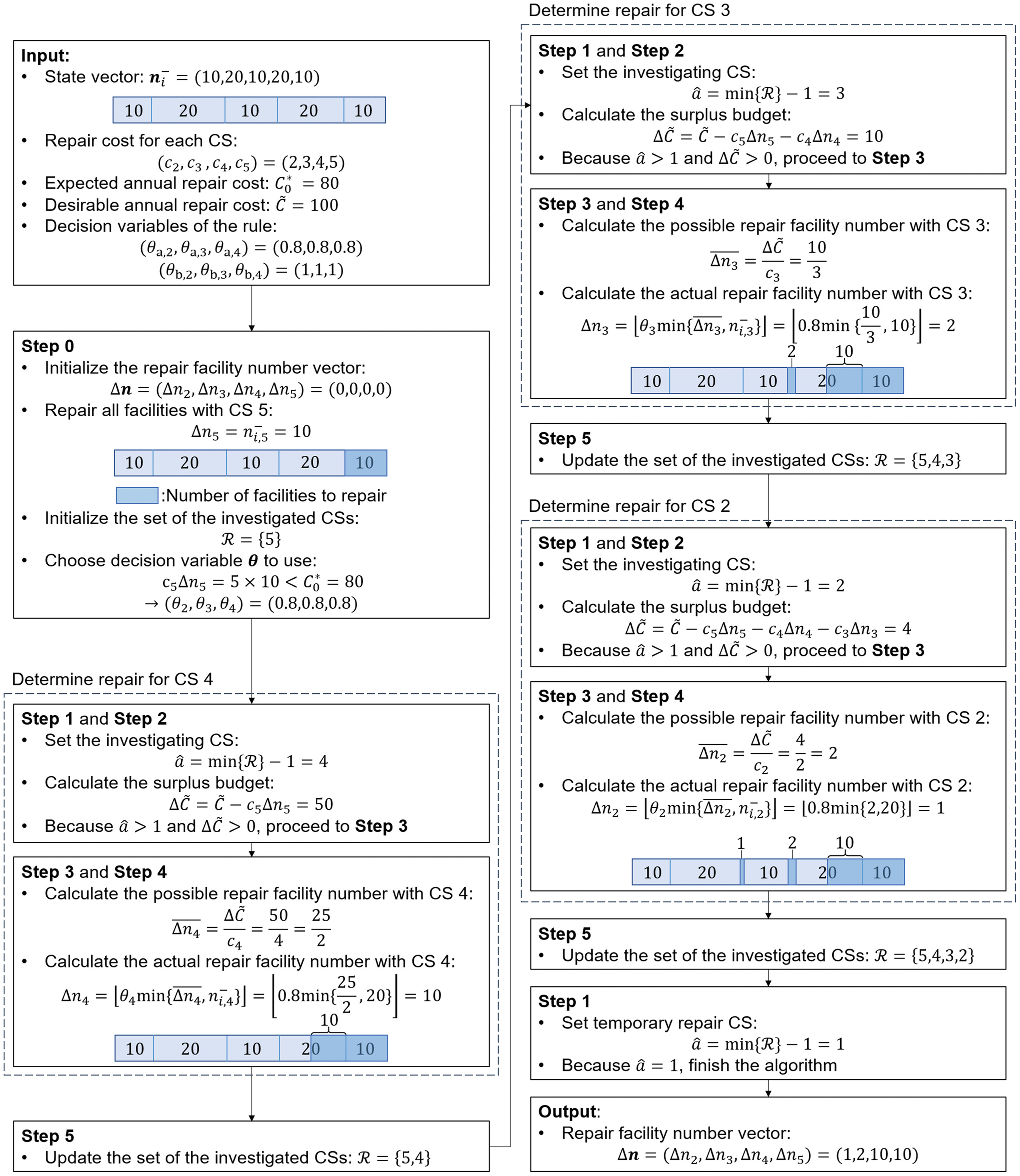
At any time point with given state vector , the number of facilities to repair for each CS is found based on the preventive repair rule with variables , , and by the following algorithm.
Step 0: Initialize the set of the investigated CSs as and the repair facility number vector . Set the decision variable as
(42)
Step 1: Set the investigating CS as . If, finish the algorithm.
Step 2: Calculate the surplus budget as . If the surplus budget , finish the algorithm.
Step 3: Calculate the possible repair facility number with CS as a real number as
(43)
Step 4: Calculate the actual repair facility number in an integer aswhere = floor function.
(44)
Step 5: Update the set of the investigated CSs as , and return to Step 1.
An example of a specific procedure for determining for a given is shown in Fig. 2. With the repair facility number vector given by the algorithm, we can determine the elements of the operator matrix as follows:
(45)
With the above procedure, we can calculate given and . This allows us to derive the cost function on the basis of the preventive repair rule–based policy as follows:where = occurrence probability of the state vector before repair in the steady state with given . The preventive repair rule–based policy only comprises decision variables, and the size of the search space of the decision variables becomes . The operator indicates the number of elements (the cardinality) of the set. Thus, we can find an optimal preventive repair rule–based policy with the combinations of the decision variables to minimize the cost function by calculating the cost function with the Monte Carlo simulation with sufficiently many iterations for all possible combinations of the decision variables. In an iteration, given , the annual repair costs at time points can be calculated, and these values can be used to numerically determine the value of . Here we assume . By performing a total of simulations for each pattern of and comparing the results, the optimal value turns out to be
(46)
(47)
(48)
(49)
In the numerical study in this paper, we do not specify to derive the preventive repair rule–based policy, but calculate the expected value and variance in annual repair costs by simulation for each and then compare the results to extract the Pareto frontier of .
Numerical Study
The efficacy of the two proposed methods is demonstrated by applying them for solving two types of infrastructure systems with different sizes: (1) a small-scale system with (Case 1); and (2) a large-scale system with (Case 2). In Case 1, the repair policy derived with the exact solution method and the one with the proposed approximation method are compared. In Case 2, the applicability of the proposed approximation method to a large-scale system is discussed. The decision variables used in the numerical study are given in Table 1. All costs and times used here are defined in an arbitrary monetary unit and an arbitrary time unit, and we do not specify these units. To reduce the computational load, we set the constraint ; thus, the search space of decision variables for the preventive repair rule–based policy is . To determine an optimal preventive rule–based repair policy, the annual repair costs and their variance are calculated using time point management process simulation, and the mean value over simulations is used to determine the corresponding value of the objective function.
| Case 1 | Case 2 | |
|---|---|---|
| Number of facilities: | 20 | 100 |
| Number of CSs: | 4 | 4 |
| Unit time interval: | 1 | 1 |
| Discount factor: | 0.04 | 0.04 |
| Investigated relative weights: | ||
| CS after repair of CS 2: | 1 | 1 |
| Repair cost for CS 2: | 300 | 300 |
| CS after repair of CS 3: | 2 | 2 |
| Repair cost for CS 3: | 400 | 400 |
| CS after repair of CS 4: | 1 | 1 |
| Repair cost for CS 4: | 1,000 | 1,000 |
| Markov transition probability matrix: | 0.6922 | |
| State space of | ||
| State space of | ||
| State space of | ||
| State space of | {0, 1} | {0, 1} |
| State space of | {0, 1} | {0, 1} |
Case 1: Small-Scale System
Optimal Policy: Exact Solution
The optimal repair policies for each are derived with the exact solution method for a small-scale system. In Table 2, the expected value of and variance in the annual repair cost when the optimal solution is adopted for each case of and are shown. When , only cost minimization is considered, and in this input condition case, , such that ; that is, the corrective repair policy that only repairs all facilities with CS 4, is the optimal solution. Note that even if the optimal solution for cost minimization is not the corrective repair policy, the variance in annual repair costs would be reduced by the proposed exact or approximate solution methods. From the table, it can be confirmed that the proposed exact solution method can derive a repair policy that reduces the variance in annual repair costs depending on. In Table 3, the exact solution for the case is listed. However, we do not list where . The numbers of repaired facilities are calculated as . The repair policy in the table is clearly different from the corrective repair policy (i.e., the optimal solution in the cost minimization case), and it indicates that the variance in the annual repair cost can be reduced by repairing not only facilities with CS 4 but also those with CSs 3 and 2.
| Annual repair cost | 1,915.10 | 1,937.41 |
| Variance | 1,731,719 | 1,124,484 |
| Number of repaired facilities | |
|---|---|
| (0,0,19,1) | (0,0,2,1) |
| (0,0,20,0) | (0,0,5,0) |
| (0,1,18,1) | (0,0,2,1) |
| (0,1,19,0) | (0,0,4,0) |
| (0,2,17,1) | (0,0,2,1) |
| (0,2,18,0) | (0,0,4,0) |
| (0,3,16,1) | (0,0,2,1) |
| (0,3,17,0) | (0,0,4,0) |
| (0,4,15,1) | (0,0,1,1) |
| (0,4,16,0) | (0,0,4,0) |
| (0,5,14,1) | (0,0,1,1) |
| (0,5,15,0) | (0,1,3,0) |
| (0,6,13,1) | (0,0,1,1) |
| (0,6,14,0) | (0,2,2,0) |
| (0,7,12,1) | (0,1,0,1) |
| (0,7,13,0) | (0,3,1,0) |
| (0,8,11,1) | (0,1,0,1) |
| (0,8,12,0) | (0,4,0,0) |
| (0,9,10,1) | (0,1,0,1) |
| (0,9,11,0) | (0,4,0,0) |
| (0,10,9,1) | (0,1,0,1) |
| (0,10,10,0) | (0,4,0,0) |
| (0,11,8,1) | (0,1,0,1) |
| (0,11,9,0) | (0,4,0,0) |
| (0,12,7,1) | (0,1,0,1) |
| (0,12,8,0) | (0,4,0,0) |
| (0,13,6,1) | (0,1,0,1) |
| (0,13,7,0) | (0,4,0,0) |
| (0,14,6,0) | (0,4,0,0) |
| (0,15,5,0) | (0,4,0,0) |
| (0,16,4,0) | (0,3,0,0) |
| (0,17,3,0) | (0,3,0,0) |
| (0,18,2,0) | (0,3,0,0) |
| (0,19,1,0) | (0,3,0,0) |
| (0,20,0,0) | (0,3,0,0) |
| (1,0,18,1) | (0,0,2,1) |
| (1,0,19,0) | (0,0,4,0) |
| (1,1,17,1) | (0,0,2,1) |
| (1,1,18,0) | (0,0,4,0) |
| (1,2,16,1) | (0,0,2,1) |
| (1,2,17,0) | (0,0,4,0) |
| (1,3,15,1) | (0,0,1,1) |
| (1,3,16,0) | (0,1,3,0) |
| (1,4,14,1) | (0,0,1,1) |
| (1,4,15,0) | (0,1,3,0) |
| (1,5,13,1) | (0,0,1,1) |
| (1,5,14,0) | (0,2,2,0) |
| (1,6,12,1) | (0,1,0,1) |
| (1,6,13,0) | (0,3,1,0) |
| (1,7,11,1) | (0,1,0,1) |
| (1,7,12,0) | (0,4,0,0) |
| (1,8,10,1) | (0,1,0,1) |
| (1,8,11,0) | (0,4,0,0) |
| (1,9,9,1) | (0,1,0,1) |
| (1,9,10,0) | (0,4,0,0) |
| (1,10,8,1) | (0,1,0,1) |
| (1,10,9,0) | (0,4,0,0) |
| (1,11,7,1) | (0,1,0,1) |
| (1,11,8,0) | (0,4,0,0) |
| (1,12,7,0) | (0,4,0,0) |
| (1,13,6,0) | (0,4,0,0) |
| (1,14,5,0) | (0,3,0,0) |
| (1,15,4,0) | (0,3,0,0) |
| (1,16,3,0) | (0,3,0,0) |
| (1,17,2,0) | (0,3,0,0) |
| (1,18,1,0) | (0,3,0,0) |
| (1,19,0,0) | (0,3,0,0) |
| (2,0,17,1) | (0,0,2,1) |
| (2,0,18,0) | (0,0,4,0) |
| (2,1,16,1) | (0,0,2,1) |
| (2,1,17,0) | (0,0,4,0) |
| (2,2,15,1) | (0,0,1,1) |
| (2,2,16,0) | (0,1,3,0) |
| (2,3,14,1) | (0,0,1,1) |
| (2,3,15,0) | (0,1,3,0) |
| (2,4,13,1) | (0,0,1,1) |
| (2,4,14,0) | (0,2,2,0) |
| (2,5,12,1) | (0,1,0,1) |
| (2,5,13,0) | (0,3,1,0) |
| (2,6,11,1) | (0,1,0,1) |
| (2,6,12,0) | (0,4,0,0) |
| (2,7,10,1) | (0,1,0,1) |
| (2,7,11,0) | (0,4,0,0) |
| (2,8,9,1) | (0,1,0,1) |
| (2,8,10,0) | (0,4,0,0) |
| (2,9,8,1) | (0,1,0,1) |
| (2,9,9,0) | (0,4,0,0) |
| (2,10,8,0) | (0,4,0,0) |
| (2,11,7,0) | (0,4,0,0) |
| (2,12,6,0) | (0,3,0,0) |
| (2,13,5,0) | (0,3,0,0) |
| (2,14,4,0) | (0,3,0,0) |
| (2,15,3,0) | (0,3,0,0) |
| (2,16,2,0) | (0,3,0,0) |
| (2,17,1,0) | (0,3,0,0) |
| (2,18,0,0) | (0,3,0,0) |
| (3,0,16,1) | (0,0,1,1) |
| (3,0,17,0) | (0,0,4,0) |
| (3,1,15,1) | (0,0,1,1) |
| (3,1,16,0) | (0,1,3,0) |
| (3,2,14,1) | (0,0,1,1) |
| (3,2,15,0) | (0,2,2,0) |
| (3,3,13,1) | (0,0,1,1) |
| (3,3,14,0) | (0,2,2,0) |
| (3,4,12,1) | (0,1,0,1) |
| (3,4,13,0) | (0,3,1,0) |
| (3,5,11,1) | (0,1,0,1) |
| (3,5,12,0) | (0,4,0,0) |
| (3,6,10,1) | (0,1,0,1) |
| (3,6,11,0) | (0,4,0,0) |
| (3,7,9,1) | (0,1,0,1) |
| (3,7,10,0) | (0,4,0,0) |
| (3,8,8,1) | (0,1,0,1) |
| (3,8,9,0) | (0,4,0,0) |
| (3,9,8,0) | (0,4,0,0) |
| (3,10,7,0) | (0,4,0,0) |
| (3,11,6,0) | (0,3,0,0) |
| (3,12,5,0) | (0,3,0,0) |
| (3,13,4,0) | (0,3,0,0) |
| (3,14,3,0) | (0,3,0,0) |
| (3,15,2,0) | (0,3,0,0) |
| (3,16,1,0) | (0,3,0,0) |
| (3,17,0,0) | (0,3,0,0) |
| (4,0,15,1) | (0,0,1,1) |
| (4,0,16,0) | (0,0,3,0) |
| (4,1,14,1) | (0,0,1,1) |
| (4,1,15,0) | (0,0,3,0) |
| (4,2,13,1) | (0,0,1,1) |
| (4,2,14,0) | (0,2,2,0) |
| (4,3,12,1) | (0,1,0,1) |
| (4,3,13,0) | (0,3,1,0) |
| (4,4,11,1) | (0,1,0,1) |
| (4,4,12,0) | (0,4,0,0) |
| (4,5,10,1) | (0,1,0,1) |
| (4,5,11,0) | (0,4,0,0) |
| (4,6,9,1) | (0,1,0,1) |
| (4,6,10,0) | (0,4,0,0) |
| (4,7,9,0) | (0,4,0,0) |
| (4,8,8,0) | (0,4,0,0) |
| (4,9,7,0) | (0,3,0,0) |
| (4,10,6,0) | (0,3,0,0) |
| (4,11,5,0) | (0,3,0,0) |
| (4,12,4,0) | (0,3,0,0) |
| (4,13,3,0) | (0,3,0,0) |
| (4,14,2,0) | (0,3,0,0) |
| (4,15,1,0) | (0,3,0,0) |
| (4,16,0,0) | (0,2,0,0) |
| (5,0,14,1) | (0,0,1,1) |
| (5,0,15,0) | (0,0,3,0) |
| (5,1,13,1) | (0,0,1,1) |
| (5,1,14,0) | (0,1,2,0) |
| (5,2,12,1) | (0,1,0,1) |
| (5,2,13,0) | (0,1,2,0) |
| (5,3,11,1) | (0,1,0,1) |
| (5,3,12,0) | (0,3,1,0) |
| (5,4,10,1) | (0,1,0,1) |
| (5,4,11,0) | (0,4,0,0) |
| (5,5,10,0) | (0,4,0,0) |
| (5,6,9,0) | (0,4,0,0) |
| (5,7,8,0) | (0,3,0,0) |
| (5,8,7,0) | (0,3,0,0) |
| (5,9,6,0) | (0,3,0,0) |
| (5,10,5,0) | (0,3,0,0) |
| (5,11,4,0) | (0,3,0,0) |
| (5,12,3,0) | (0,3,0,0) |
| (5,13,2,0) | (0,3,0,0) |
| (5,14,1,0) | (0,3,0,0) |
| (5,15,0,0) | (0,2,0,0) |
| (6,0,13,1) | (0,0,1,1) |
| (6,0,14,0) | (0,0,3,0) |
| (6,1,12,1) | (0,1,0,1) |
| (6,1,13,0) | (0,1,2,0) |
| (6,2,11,1) | (0,1,0,1) |
| (6,2,12,0) | (0,2,1,0) |
| (6,3,10,1) | (0,1,0,1) |
| (6,3,11,0) | (0,3,0,0) |
| (6,4,10,0) | (0,4,0,0) |
| (6,5,9,0) | (0,3,0,0) |
| (6,6,8,0) | (0,3,0,0) |
| (6,7,7,0) | (0,3,0,0) |
| (6,8,6,0) | (0,3,0,0) |
| (6,9,5,0) | (0,3,0,0) |
| (6,10,4,0) | (0,3,0,0) |
| (6,11,3,0) | (0,3,0,0) |
| (6,12,2,0) | (0,3,0,0) |
| (6,13,1,0) | (0,2,0,0) |
| (6,14,0,0) | (0,2,0,0) |
| (7,0,13,0) | (0,0,3,0) |
| (7,1,11,1) | (0,1,0,1) |
| (7,1,12,0) | (0,1,2,0) |
| (7,2,11,0) | (0,2,1,0) |
| (7,3,10,0) | (0,3,0,0) |
| (7,4,9,0) | (0,3,0,0) |
| (7,5,8,0) | (0,3,0,0) |
| (7,6,7,0) | (0,3,0,0) |
| (7,7,6,0) | (0,3,0,0) |
| (7,8,5,0) | (0,3,0,0) |
| (7,9,4,0) | (0,3,0,0) |
| (7,10,3,0) | (0,3,0,0) |
| (7,11,2,0) | (0,2,0,0) |
| (7,12,1,0) | (0,2,0,0) |
| (7,13,0,0) | (0,2,0,0) |
| (8,0,12,0) | (0,0,2,0) |
| (8,1,11,0) | (0,1,2,0) |
| (8,2,10,0) | (0,2,1,0) |
| (8,3,9,0) | (0,3,0,0) |
| (8,4,8,0) | (0,3,0,0) |
| (8,5,7,0) | (0,3,0,0) |
| (8,6,6,0) | (0,3,0,0) |
| (8,7,5,0) | (0,3,0,0) |
| (8,8,4,0) | (0,3,0,0) |
| (8,9,3,0) | (0,3,0,0) |
| (8,10,2,0) | (0,2,0,0) |
| (8,11,1,0) | (0,2,0,0) |
| (8,12,0,0) | (0,2,0,0) |
| (9,0,11,0) | (0,0,2,0) |
| (9,1,10,0) | (0,1,1,0) |
| (9,2,9,0) | (0,2,0,0) |
| (9,3,8,0) | (0,3,0,0) |
| (9,4,7,0) | (0,3,0,0) |
| (9,5,6,0) | (0,3,0,0) |
| (9,6,5,0) | (0,3,0,0) |
| (9,7,4,0) | (0,3,0,0) |
| (9,8,3,0) | (0,2,0,0) |
| (9,9,2,0) | (0,2,0,0) |
| (9,10,1,0) | (0,2,0,0) |
| (9,11,0,0) | (0,2,0,0) |
| (10,0,10,0) | (0,0,2,0) |
| (10,1,9,0) | (0,1,1,0) |
| (10,2,8,0) | (0,2,0,0) |
| (10,3,7,0) | (0,3,0,0) |
| (10,4,6,0) | (0,3,0,0) |
| (10,5,5,0) | (0,3,0,0) |
| (10,6,4,0) | (0,2,0,0) |
| (10,7,3,0) | (0,2,0,0) |
| (10,8,2,0) | (0,2,0,0) |
| (10,9,1,0) | (0,2,0,0) |
| (10,10,0,0) | (0,2,0,0) |
| (11,0,9,0) | (0,0,2,0) |
| (11,1,8,0) | (0,1,1,0) |
| (11,2,7,0) | (0,2,0,0) |
| (11,3,6,0) | (0,3,0,0) |
| (11,4,5,0) | (0,2,0,0) |
| (11,5,4,0) | (0,2,0,0) |
| (11,6,3,0) | (0,2,0,0) |
| (11,7,2,0) | (0,2,0,0) |
| (11,8,1,0) | (0,2,0,0) |
| (11,9,0,0) | (0,2,0,0) |
| (12,0,8,0) | (0,0,1,0) |
| (12,1,7,0) | (0,1,1,0) |
| (12,2,6,0) | (0,2,0,0) |
| (12,3,5,0) | (0,2,0,0) |
| (12,4,4,0) | (0,2,0,0) |
| (12,5,3,0) | (0,2,0,0) |
| (12,6,2,0) | (0,2,0,0) |
| (12,7,1,0) | (0,2,0,0) |
| (12,8,0,0) | (0,2,0,0) |
| (13,0,7,0) | (0,0,1,0) |
| (13,1,6,0) | (0,1,0,0) |
| (13,2,5,0) | (0,2,0,0) |
| (13,3,4,0) | (0,2,0,0) |
| (13,4,3,0) | (0,2,0,0) |
| (13,5,2,0) | (0,2,0,0) |
| (13,6,1,0) | (0,2,0,0) |
| (13,7,0,0) | (0,2,0,0) |
| (14,0,6,0) | (0,0,1,0) |
| (14,1,5,0) | (0,1,0,0) |
| (14,2,4,0) | (0,2,0,0) |
| (14,3,3,0) | (0,2,0,0) |
| (14,4,2,0) | (0,2,0,0) |
| (14,5,1,0) | (0,2,0,0) |
| (14,6,0,0) | (0,1,0,0) |
| (15,0,5,0) | (0,0,1,0) |
| (15,1,4,0) | (0,1,0,0) |
| (15,2,3,0) | (0,2,0,0) |
| (15,3,2,0) | (0,2,0,0) |
| (15,4,1,0) | (0,2,0,0) |
| (15,5,0,0) | (0,1,0,0) |
| (16,1,3,0) | (0,1,0,0) |
| (16,2,2,0) | (0,2,0,0) |
| (16,3,1,0) | (0,1,0,0) |
| (16,4,0,0) | (0,1,0,0) |
| (17,1,2,0) | (0,1,0,0) |
| (17,2,1,0) | (0,1,0,0) |
| (17,3,0,0) | (0,1,0,0) |
| (18,1,1,0) | (0,1,0,0) |
| (18,2,0,0) | (0,1,0,0) |
| (19,1,0,0) | (0,1,0,0) |
Preventive Repair Rule–Based Policy: Approximate Solution
The preventive repair rule–based policy expresses the implementation of preventive repair in the exact solution as a rule independent of . The actual number of facilities to be repaired depends on , but is independent of . In Table 4, we list decision variables in the preventive repair rule–based policies on the Pareto frontier with the expected value of and variance in the annual repair cost as evaluation indices. Selecting , which corresponds to a desirable pair of annual repair cost and variance, from the results in the table and then deciding on the number of facilities to be repaired on the basis of the selected is simpler than using the exact solution shown in Table 3. For example, if we select , the variance in the annual repair cost can be reduced from 1,731,719 (the cost minimization case) to 1,437,585 by following the simplified rule as follows: “At each time point, besides repairing all facilities with CS 4, repair up to 16.6% of facilities with CS 3 and up to 37.5% of facilities with CS 2 under the condition that the annual repair cost is less than or equal to .”
| Expected value of annual cost | Variance in annual cost | ||||
|---|---|---|---|---|---|
| 1,915.10 | 1,731,719 | 0 | 0 | 0 | 1 |
| 1,916.59 | 1,668,589 | 1.3 | 0.125 | 0 | 0 |
| 1,919.67 | 1,560,029 | 1.1 | 0.25 | 0 | 1 |
| 1,920.18 | 1,552,960 | 0.7 | 0.375 | 0 | 0 |
| 1,924.17 | 1,437,585 | 0.9 | 0.375 | 0.1666 | 1 |
| 1,925.64 | 1,394,551 | 0.7 | 0.625 | 0.1666 | 1 |
| 1,931.34 | 1,251,267 | 0.7 | 0.75 | 0.1666 | 1 |
| 1,931.34 | 1,250,963 | 0.7 | 0.75 | 0 | 1 |
| 1,935.37 | 1,223,518 | 1.1 | 0.375 | 0 | 0 |
| 1,937.40 | 1,169,135 | 0.9 | 0.5 | 0 | 1 |
| 1,941.99 | 1,064,926 | 1.1 | 0.5 | 0 | 1 |
| 1,942.48 | 1,064,561 | 1.1 | 0.5 | 0 | 0 |
| 1,943.05 | 1,040,970 | 0.9 | 0.625 | 0 | 0 |
| 1,943.16 | 1,040,684 | 0.9 | 0.625 | 0.1666 | 1 |
| 1,949.10 | 926,753 | 0.9 | 0.75 | 0.1666 | 0 |
| 1,949.29 | 926,330 | 0.9 | 0.75 | 0 | 0 |
| 1,951.59 | 869,595 | 0.7 | 1 | 0 | 1 |
| 1,959.49 | 824,875 | 1.1 | 0.625 | 0.1666 | 1 |
| 1,959.51 | 824,670 | 1.1 | 0.625 | 0 | 1 |
| 1,967.76 | 704,391 | 1.1 | 0.75 | 0 | 1 |
| 1,970.55 | 662,213 | 0.9 | 0.875 | 0 | 0 |
| 1,970.57 | 661,568 | 0.9 | 0.875 | 0.1666 | 0 |
| 1,975.62 | 586,581 | 0.9 | 1 | 0.1666 | 0 |
| 1,975.76 | 585,896 | 0.9 | 1 | 0.1666 | 1 |
| 1,988.61 | 543,009 | 1.1 | 0.875 | 0.1666 | 0 |
| 1,989.96 | 537,530 | 1.1 | 0.875 | 0.1666 | 1 |
| 1,989.98 | 537,472 | 1.1 | 0.875 | 0 | 1 |
| 1,991.65 | 533,515 | 0.9 | 0.875 | 0.3333 | 1 |
| 1,995.54 | 516,884 | 1.1 | 0.75 | 0.3333 | 0 |
| 1,995.73 | 515,989 | 1.1 | 0.75 | 0.3333 | 1 |
| 2,004.12 | 423,843 | 1.1 | 1 | 0 | 0 |
| 2,008.14 | 400,860 | 1.1 | 1 | 0.1666 | 1 |
| 2,021.85 | 364,523 | 1.1 | 0.875 | 0.3333 | 0 |
| 2,023.30 | 352,748 | 1.1 | 0.875 | 0.3333 | 1 |
| 2,042.98 | 295,058 | 1.1 | 1 | 0.3333 | 0 |
| 2,051.06 | 243,546 | 1.1 | 1 | 0.3333 | 1 |
| 2,080.84 | 227,875 | 1.1 | 0.75 | 0.5 | 1 |
| 2,102.87 | 197,851 | 0.9 | 1 | 0.6666 | 0 |
| 2,103.23 | 197,382 | 1.3 | 0.75 | 0.3333 | 1 |
| 2,103.97 | 190,335 | 0.9 | 1 | 0.6666 | 1 |
| 2,108.35 | 185,855 | 1.1 | 0.875 | 0.5 | 0 |
| 2,109.56 | 185,125 | 1.3 | 0.625 | 0.5 | 1 |
| 2,111.69 | 154,639 | 1.1 | 0.875 | 0.5 | 1 |
| 2,146.39 | 129,551 | 1.3 | 0.75 | 0.5 | 1 |
| 2,154.58 | 116,210 | 1.1 | 1 | 0.5 | 1 |
Here we check the variation in the distribution of the annual repair cost by considering the cost leveling. Figs. 3 and 4 are histograms of annual repair costs for the preventive repair rule–based policies of (minimal cost and maximum variance case, which is equivalent to the case in the exact solution method) and (minimal variance and maximum cost case), respectively. These annual repair costs are calculated by simulation using the preventive repair rule–based policies as input. Comparing the histogram for the minimal variance and maximum cost case with the one for the minimal cost and maximum variance case, we find that the variation in both the upper and lower sides from the expected annual repair cost is reduced. This implies that considering cost-leveling yields (1) the effect by adjusting the annual repair cost closer to the desirable annual repair cost when the annual repair cost is low with corrective repair only at a time point; and (2) the effect by advancing some of the future repairs to prevent the concentration of repairs at one time point in the future. The latter is a desynchronization of the repair time points. Conversely, synchronization may be desirable in some cases where economies of scale exist in repair costs (e.g., Mizutani et al. 2020). Here we assume situations where the benefits of economies of scale due to the synchronization are relatively small, which happens for instance when individual facilities are geographically distant from each other.


In Figs. 5 and 6, variations in annual repair costs over a 20-year time horizon are shown for each situation in Figs. 3 and 4, respectively. In each figure, we illustrate the results of each of 1,000 simulations, with all initial CSs set to 1. By comparing these figures, it can be confirmed that the proposed method can restrain the variation in actual annual repair costs, which means that it can flexibly respond to annual budget constraints. Nevertheless, since a stochastic deterioration process is assumed here, it is theoretically impossible to completely prevent an annual repair cost from exceeding the budget. This corresponds to the occurrence possibility of sudden and unexpected deterioration events in actual asset management. To address this issue, it is desirable to prepare an additional budgeting system, such as insurance, but a detailed discussion of this is beyond the scope of this study.


Now let us look at the features of the solutions of the preventive repair rule–based policy. The solutions containing are extracted from Table 4 and shown in Fig. 7. Looking at the changes in the decision variables from left to the right, we observe that the value of increases first; then increases, and lastly increases. This indicates that the implementation of preventive repair tends to increase as the variance in the annual repair cost decreases. Additionally, for the present input conditions, it is suggested that , , and have a greater impact on the order of controlling variance while preventing cost increases.

Comparison of Solution Methods
We now review and compare the Pareto frontiers of the exact and approximate solutions. In Fig. 8, the Pareto frontiers on the two-dimensional plane of the expected value of the annual repair cost and its variance, derived respectively by the two solution methods, are shown. The Pareto frontier for the exact solution is calculated by simulations using the optimal repair policy for each as input information. A trade-off relation can be observed on both Pareto frontiers. This means that cost leveling can be achieved by incurring additional repair costs. Furthermore, this result can be interpreted as a quantification of the additional incremental repair costs that are caused by the current single-year budget principle.

From Fig. 8, we see the similarity between the two Pareto frontiers. Particularly, as can be seen in the upper left of the graph, the consistency between the two solutions is remarkably high in the range where the expected annual repair cost is relatively small. Conversely, as we see in the lower right of the graph, if we attempt to reduce the variance substantially, the similarity between them diminishes slightly. This is presumably because the implementation method of preventive repair for variance reduction is complicated and there is a limit to the exact representation of the optimal solution using an approximate one.
Fig. 8 also shows the Pareto frontier obtained with a genetic algorithm. The settings of the genetic algorithm are the selection method: roulette wheel selection; the crossover method: two-point crossover; the mutation method: bit string mutation; maximum generation: 1,000; population size: 60; stopping condition for the algorithm: if the relative change in the mean of the objective function values falls below 200, or if the number of generations reaches its maximum value. In the figure, the Pareto frontier of the genetic algorithm is located in the upper right compared with the Pareto frontier of the exact solution and the preventive repair rule–based policy; that is, the significance of the proposed method can be confirmed from the figure. It is possible that better solutions can be derived by modifying the settings of the genetic algorithm or by using more advanced genetic algorithms, but this is beyond the scope of this study. Note that we also attempte to apply the genetic algorithm to the large-scale system in Case 2, but the size of the repair policy vector is so large that even setting the vector in the programming software is not feasible.
Case 2: Large-Scale System
The exact solution method cannot be directly applied to the large-scale system because of the computational complexity. One possible approximate method based on the exact solution is to decompose the whole system into subsystems whose scales are sufficiently small to allow deriving the exact solution and then to apply the exact solution within the subsystems while leaving the decision-making between the subsystems independent. Conversely, the approximate solution method with the preventive repair rule–based policy can be directly applied to large-scale systems because the search space for decision variables is independent of the number of facilities. Here, we compare (1) the results of decomposing a large-scale system with into five subsystems with and applying the exact solution to each subsystem independently; and (2) the results of applying the approximate solution with the preventive repair rule–based policy. In Fig. 9, the Pareto frontiers derived by the two methods are shown. The Pareto frontier of the preventive repair rule–based policy is located on the lower left side compared with that of the exact solution applied to each subsystem, thus confirming the superiority of the preventive repair rule–based policy.

Summary and Future Tasks
In this study, we first proposed a model for deriving the optimal repair policy for the infrastructure system considering cost minimization and cost leveling. It applies a Markov decision process to consider stochastic deterioration processes. We also proposed two solution methods for solving this model, an exact one and an approximated one on the basis of the preventive repair rule. Numerical results illustrate the theoretical achievements, showing in particular that (1) the proposed model and the exact solution method can be used to determine the Pareto frontier between life cycle cost and variance in the annual repair cost in small-scale systems; (2) the preventive repair rule–based policy provides a near-optimal solution for small-scale systems; and (3) a superior repair policy for aggregating the optimal solutions independently found for each decomposed subsystem can be determined as the preventive repair rule–based policy for large-scale systems.
The following are envisioned future tasks related to this study:
•
Further investigation into the index for the dispersion of annual repair costs is necessary. In this study, the weighted sum of the annual repair cost and its variance was used as the objective function of the proposed optimization problem. One could consider using other indices instead of the variance, such as standard deviation, or even applying a nonlinear cost function. Additionally, it is important to continuously verify the semantic interpretation of the weight and to set it according to various real-world situations.
•
After setting a preventive repair rule using trial and error as in this study, it is important to consider various other possibilities to formulate this rule. For example, as the deterioration process of the system or the unit cost of repair changes, it may be desired to modify the definition of the threshold in Eq. (40), or two different ( and ) may not be needed. Thus, it is necessary to continuously examine what type of preventive repair rule is appropriate for a given situation.
•
The budget system must be verified and improved using the analysis results of the proposed methodology. In this study, we derived a trade-off relation between the annual repair cost and its variance. This result should be reflected in the setting of budget principles and periods (single year or multiple years) and budget amounts.
•
It is desirable to develop a cost-leveling methodology to address heterogeneous asset systems. This makes the combinatorial explosion problem more complex because it is necessary to determine intervention policies based not only on the state vector but also on information on heterogeneity (which assets have what heterogeneity and which CSs). In this regard, the proposed methodology might be improved by establishing a simplified rule that consolidates the observed CS and heterogeneity information.
Appendix. Problem Formulation and Determination of Repair Policy
| Symbol | Definition |
|---|---|
| “Discrete Time Axis” subsection | |
| Time point | |
| Identification number of each time point | |
| Fixed interval between time points and | |
| Set of natural numbers including 0 (State space of ) | |
| Set of time points | |
| “State Vector” subsection | |
| Number of facilities in system | |
| Number of CSs for single facility | |
| State space of CS | |
| State vector of system at time point | |
| Number of facilities with CS at time point | |
| State vectors of system at time point before/after repair | |
| Number of possible patterns for state vector | |
| State space of identification number of each state vector | |
| Identification number of each state vector | |
| State space of state vector | |
| th state vector in | |
| Number of facilities with CS when state vector is (th element of ) | |
| “Deterioration Process” subsection | |
| Markov transition probability of CS change from to between and | |
| CSs at time point before/after repair | |
| Markov transition probability matrix of single facility | |
| State variation matrix from to | |
| Number of facilities where CSs change from to when state vector changes from to | |
| Occurrence probability of state variation matrix | |
| Set of all possible state variation matrices | |
| Transition probability of state vector from to | |
| Transition probability matrix for state vectors (Deterioration of entire system) | |
| “Repair Process” subsection | |
| CS after repair when facility with CS repaired | |
| Identification number of each repair policy | |
| Set of repair policies when number of facilities in system is | |
| Operator matrix that converts state vector before repair to that after repair | |
| Ratio of number of facilities with CS before repair whose CSs become after repair to | |
| Deterministic transition matrix of state vector by repair policy (Repair of entire system) | |
| element of | |
| “Objective Function” subsection | |
| Occurrence probability vector of state vector before repair at time point with given repair policy | |
| Occurrence probability that state vector before repair is at time point with given repair policy (th element of ) | |
| Occurrence probability vector of state vector when deterioration and repair converge into steady state with given repair policy | |
| Occurrence probability that state vector before repair is when deterioration and repair converge into steady state with given repair policy (th element of ) | |
| Repair cost at time point when state vector before repair is with given repair policy | |
| Unit cost per facility to perform repair that alters CS from to | |
| Expected annual repair cost with given repair policy in steady state | |
| Variance of annual repair cost with given repair policy in steady state | |
| Cost function with given initial state vector and repair policy (discounted present value of sum of expected values of annual repair costs and their variances over infinite horizon) | |
| Expected value of input with respect to random vector | |
| Relative weight between annual repair cost and its variance | |
| Discount factor | |
| Symbol | Definition |
|---|---|
| “Optimal Policy: Exact Solution” subsection | |
| Left-hand side of Bellman equation (optimal value function) | |
| Optimal repair policy derived by exact solution method | |
| “Preventive Repair Rule–Based Policy: Approximate Solution” subsection | |
| Set of decision variables for preventive repair rule–based policy | |
| State space of | |
| Parameter (decision variable) to set desirable annual repair cost for preventive repair rule–based policy | |
| State space of | |
| Parameters (decision variables) determining ratio of preventive repair for each CS for preventive repair rule–based policy | |
| th elements of | |
| State spaces of | |
| Ratio of number of facilities with CS before repair whose CSs become after repair to , under preventive repair rule–based policy with given decision variable set | |
| Operator matrix that converts state vector before repair to that after repair, under preventive repair rule–based policy with given decision variable set | |
| Optimal preventive repair rule–based policy | |
| Optimal value of | |
| Optimal values of | |
| Optimal repair policy obtained via Eq. (38) with | |
| Expected annual repair cost when optimal repair policy is adopted for case where is set in Eq. (38) (used in algorithm) | |
| Desirable annual repair cost (used in algorithm) | |
| Set of investigated CSs (used in algorithm) | |
| Repair facility number vector (used in algorithm) | |
| Number of facilities with CS to repair (th element of ) (used in algorithm) | |
| Parameters determining ratio of preventive repair for each CS, determined according to , , and magnitude relation between and (used in algorithm) | |
| th element of (used in algorithm) | |
| Investigating CS (used in algorithm) | |
| Surplus budget (used in algorithm) | |
| Possible repair facility number with CS as real number (used in algorithm) | |
| Actual repair facility number with CS in integer (used in algorithm) | |
| Cost function for CS with given decision variable set under preventive repair rule–based policy | |
| Occurrence probability of state vector before repair in steady state with given preventive repair rule–based policy | |
| Repair cost at time point when state vector before repair is with given preventive repair rule–based policy | |
| Expected annual repair cost with given preventive repair rule–based policy in steady state | |
| Number of iterations for Monte Carlo simulation (Sufficiently large number) | |
| Number of time points for Monte Carlo simulation (sufficiently large number) | |
Data Availability Statement
All data, models, and code that support the findings of this study are available from the corresponding author upon reasonable request.
Acknowledgments
This work was supported by the Japan Society for the Promotion of Science (JSPS) KAKENHI (Grant Nos. JP20H02264 and JP19H00777).
References
Boyles, S. D., Z. Zhang, and S. T. Waller. 2010. “Optimal maintenance and repair policies under nonlinear preferences.” J. Infrastruct. Syst. 16 (1): 11–20. https://doi.org/10.1061/(ASCE)1076-0342(2010)16:1(11).
Brühwiler, E., and B. Adey. 2005. “Improving the consideration of life-cycle costs in bridge decision-making in Switzerland.” Struct. Infrastruct. Eng. 1 (2): 145–157. https://doi.org/10.1080/15732470500030562.
Carvalho, T. P., F. A. Soares, R. Vita, R. D. P. Francisco, J. P. Basto, and S. G. Alcalá. 2019. “A systematic literature review of machine learning methods applied to predictive maintenance.” Comput. Ind. Eng. 137 (Nov): 106024. https://doi.org/10.1016/j.cie.2019.106024.
Chan, W. T., T. F. Fwa, and C. Y. Tan. 1994. “Road-maintenance planning using genetic algorithms. I: Formulation.” J. Transp. Eng. 120 (5): 693–709. https://doi.org/10.1061/(ASCE)0733-947X(1994)120:5(693).
Christodoulou, S. E., G. Ellinas, and A. Michaelidou-Kamenou. 2010. “Minimum moment method for resource leveling using entropy maximization.” J. Constr. Eng. Manage. 136 (5): 518–527. https://doi.org/10.1061/(ASCE)CO.1943-7862.0000149.
Chu, J. C., and K. H. Huang. 2018. “Mathematical programming framework for modeling and comparing network-level pavement maintenance strategies.” Transp. Res. Part B: Methodol. 109 (Mar): 1–25. https://doi.org/10.1016/j.trb.2018.01.005.
Durango-Cohen, P. L., and P. Sarutipand. 2007. “Capturing interdependencies and heterogeneity in the management of multifacility transportation infrastructure systems.” J. Infrastruct. Syst. 13 (2): 115–123. https://doi.org/10.1061/(ASCE)1076-0342(2007)13:2(115).
Easa, S. M. 1989. “Resource leveling in construction by optimization.” J. Constr. Eng. Manage. 115 (2): 302–316. https://doi.org/10.1061/(ASCE)0733-9364(1989)115:2(302).
France-Mensah, J., W. J. O’Brien, and N. Khwaja. 2019. “Impact of multiple highway funding categories and project eligibility restrictions on pavement performance.” J. Infrastruct. Syst. 25 (1): 04018037. https://doi.org/10.1061/(ASCE)IS.1943-555X.0000458.
Friesz, T. L., and J. E. Fernandez. 1979. “A model of optimal transport maintenance with demand responsiveness.” Transp. Res. Part B: Methodol. 13 (4): 317–339. https://doi.org/10.1016/0191-2615(79)90025-0.
Fwa, T. F., C. Y. Tan, and W. T. Chan. 1994. “Road-maintenance planning using genetic algorithms. II: Analysis.” J. Transp. Eng. 120 (5): 710–722. https://doi.org/10.1061/(ASCE)0733-947X(1994)120:5(710).
Guo, F., J. Gregory, and R. Kirchain. 2020. “Incorporating cost uncertainty and path dependence into treatment selection for pavement networks.” Transp. Res. Part C: Emerging Technol. 110 (Jan): 40–55. https://doi.org/10.1016/j.trc.2019.11.015.
Harris, R. B. 1990. “Packing method for resource leveling (PACK).” J. Constr. Eng. Manage. 116 (2): 331–350. https://doi.org/10.1061/(ASCE)0733-9364(1990)116:2(331).
Hiyassat, M. A. S. 2001. “Applying modified minimum moment method to multiple resource leveling.” J. Constr. Eng. Manage. 127 (3): 192–198. https://doi.org/10.1061/(ASCE)0733-9364(2001)127:3(192).
Hu, X., C. Daganzo, and S. Madanat. 2015. “A reliability-based optimization scheme for maintenance management in large-scale bridge networks.” Transp. Res. Part C: Emerging Technol. 55 (Jun): 166–178. https://doi.org/10.1016/j.trc.2015.01.008.
Jido, M., T. Otazawa, and K. Kobayashi. 2008. “Optimal repair and inspection rules under uncertainty.” J. Infrastruct. Syst. 14 (2): 150–158. https://doi.org/10.1061/(ASCE)1076-0342(2008)14:2(150).
Kartam, N., and T. Tongthong. 1998. “An artificial neural network for resource leveling problems.” AI EDAM 12 (3): 273–287. https://doi.org/10.1017/S0890060498123053.
Kielhauser, C., B. T. Adey, and N. Lethanh. 2017. “Investigation of a static and a dynamic neighbourhood methodology to develop work programs for multiple close municipal infrastructure networks.” Struct. Infrastruct. Eng. 13 (3): 361–389. https://doi.org/10.1080/15732479.2016.1162818.
Kothari, C., J. France-Mensah, and W. J. O’Brien. 2022. “Developing a sustainable pavement management plan: Economics, environment, and social equity.” J. Infrastruct. Syst. 28 (2): 04022009. https://doi.org/10.1061/(ASCE)IS.1943-555X.0000689.
Kuhn, K. D., and S. M. Madanat. 2005. “Model uncertainty and the management of a system of infrastructure facilities.” Transp. Res. Part C: Emerging Technol. 13 (5–6): 391–404. https://doi.org/10.1016/j.trc.2006.02.001.
Lee, J., and S. Madanat. 2015. “A joint bottom-up solution methodology for system-level pavement rehabilitation and reconstruction.” Transp. Res. Part B: Methodol. 78 (Aug): 106–122. https://doi.org/10.1016/j.trb.2015.05.001.
Leu, S. S., C. H. Yang, and J. C. Huang. 2000. “Resource leveling in construction by genetic algorithm-based optimization and its decision support system application.” Autom. Constr. 10 (1): 27–41. https://doi.org/10.1016/S0926-5805(99)00011-4.
Li, H., D. Parikh, Q. He, B. Qian, Z. Li, D. Fang, and A. Hampapur. 2014. “Improving rail network velocity: A machine learning approach to predictive maintenance.” Transp. Res. Part C: Emerging Technol. 45 (Aug): 17–26. https://doi.org/10.1016/j.trc.2014.04.013.
Li, Y., and S. Madanat. 2002. “A steady-state solution for the optimal pavement resurfacing problem.” Transp. Res. Part A: Policy Pract. 36 (6): 525–535. https://doi.org/10.1016/S0965-8564(01)00020-9.
Madanat, S. 1993. “Optimal infrastructure management decisions under uncertainty.” Transp. Res. Part C: Emerging Technol. 1 (1): 77–88. https://doi.org/10.1016/0968-090X(93)90021-7.
Madanat, S., and M. Ben-Akiva. 1994. “Optimal inspection and repair policies for infrastructure facilities.” Transp. Sci. 28 (1): 55–62. https://doi.org/10.1287/trsc.28.1.55.
Medury, A., and S. Madanat. 2013. “Incorporating network considerations into pavement management systems: A case for approximate dynamic programming.” Transp. Res. Part C: Emerging Technol. 33 (Aug): 134–150. https://doi.org/10.1016/j.trc.2013.03.003.
Mizutani, D., Y. Nakazato, and J. Lee. 2020. “Network-level synchronized pavement repair and work zone policies: Optimal solution and rule-based approximation.” Transp. Res. Part C: Emerging Technol. 120 (Nov): 102797. https://doi.org/10.1016/j.trc.2020.102797.
Ouyang, Y. 2007. “Pavement resurfacing planning for highway networks: Parametric policy iteration approach.” J. Infrastruct. Syst. 13 (1): 65–71. https://doi.org/10.1061/(ASCE)1076-0342(2007)13:1(65).
Ouyang, Y., and S. Madanat. 2004. “Optimal scheduling of rehabilitation activities for multiple pavement facilities: Exact and approximate solutions.” Transp. Res. Part A: Policy Pract. 38 (5): 347–365. https://doi.org/10.1016/j.tra.2003.10.007.
Ouyang, Y., and S. Madanat. 2006. “An analytical solution for the finite-horizon pavement resurfacing planning problem.” Transp. Res. Part B: Methodol. 40 (9): 767–778. https://doi.org/10.1016/j.trb.2005.11.001.
Sathaye, N., and S. Madanat. 2011. “A bottom-up solution for the multi-facility optimal pavement resurfacing problem.” Transp. Res. Part B: Methodol. 45 (7): 1004–1017. https://doi.org/10.1016/j.trb.2011.03.002.
Savin, D., S. Alkass, and P. Fazio. 1997. “A procedure for calculating the weight-matrix of a neural network for resource leveling.” Adv. Eng. Software 28 (5): 277–283. https://doi.org/10.1016/S0965-9978(97)00019-7.
Smilowitz, K., and S. Madanat. 2000. “Optimal inspection and maintenance policies for infrastructure networks.” Comput.-Aided Civ. Infrastruct. Eng. 15 (1): 5–13. https://doi.org/10.1111/0885-9507.00166.
Takamoto, M., N. Yamada, Y. Kobayashi, H. Nonaka, and S. Okoshi. 1995. “Zero-one quadratic programming algorithm for resource leveling of manufacturing process schedules.” Syst. Comput. Jpn. 26 (10): 68–76. https://doi.org/10.1002/scj.4690261007.
White, C. C., III, and D. J. White. 1989. “Markov decision processes.” Eur. J. Oper. Res. 39 (1): 1–16. https://doi.org/10.1016/0377-2217(89)90348-2.
Woodworth, B. M., and C. J. Willie. 1975. “A heuristic algorithm for resource leveling in multi-project, multi-resource scheduling.” Decis. Sci. 6 (3): 525–540. https://doi.org/10.1111/j.1540-5915.1975.tb01041.x.
Yoon, Y., M. Hastak, and K. Cho. 2017. “Method for generating multiple MRR solutions for application in cost-leveling models.” J. Infrastruct. Syst. 23 (3): 04016045. https://doi.org/10.1061/(ASCE)IS.1943-555X.0000351.
Yoon, Y., H. Shah, M. Hastak, and J. Lee. 2014. “Leveling process of annual budgetary requirements for pavement preservation.” J. Infrastruct. Syst. 20 (1): 04013004. https://doi.org/10.1061/(ASCE)IS.1943-555X.0000140.
Zhang, L., L. Fu, W. Gu, Y. Ouyang, and Y. Hu. 2017. “A general iterative approach for the system-level joint optimization of pavement maintenance, rehabilitation, and reconstruction planning.” Transp. Res. Part B: Methodol. 105 (Nov): 378–400. https://doi.org/10.1016/j.trb.2017.09.014.
Information & Authors
Information
Published In

Journal of Infrastructure Systems
Volume 29 • Issue 3 • September 2023
Copyright
This work is made available under the terms of the Creative Commons Attribution 4.0 International license, https://creativecommons.org/licenses/by/4.0/.
History
Received: Mar 22, 2022
Accepted: Feb 21, 2023
Published online: Jun 27, 2023
Published in print: Sep 1, 2023
Discussion open until: Nov 27, 2023
ASCE Technical Topics:
- Analysis (by type)
- Benefit cost ratios
- Business management
- Construction engineering
- Construction methods
- Engineering fundamentals
- Financial management
- Infrastructure
- Leveling
- Life cycles
- Markov process
- Mathematics
- Methodology (by type)
- Numerical analysis
- Numerical methods
- Practice and Profession
- Probability
- Rehabilitation
- Stochastic processes
Authors
Metrics & Citations
Metrics
Citations
Download citation
If you have the appropriate software installed, you can download article citation data to the citation manager of your choice. Simply select your manager software from the list below and click Download.