Steady Flow through Gated Circular Culverts: Hydraulic Operation and Experiments
This article has a reply.
VIEW THE REPLYThis article has a reply.
VIEW THE REPLYPublication: Journal of Irrigation and Drainage Engineering
Volume 149, Issue 7
Abstract
Culverts are ubiquitous hydraulic structures used in cross-drainage and agricultural water systems, especially at farm outlets in irrigation systems. Gate control adds hydraulic complexity to culvert water flow, yet it has hardly been studied. This study has two objectives: (1) to classify the operational conditions of gated culverts, and (2) to establish an experimental data set for analyzing discharge relationships based on that classification. A theoretical inlet–outlet control–based classification resulted in 22 inlet control and 19 outlet control cases, organized in 4 inlet and 5 outlet control groups. A total of 230 laboratory tests were conducted. The laboratory setup reproduced the conditions of inlet submerged with outlet in free surface (one of four inlet control groups) and all conditions except inlet in free surface with outlet submerged (four of five outlet control groups) of the inlet and outlet control groups, respectively. Comparison with existing classification schemes for gated culverts confirmed the suitability of the proposed scheme and provided further insight into flow classification. The discharge grouped by narrow ranges of gate openings was found to follow a power-law relationship of head with an exponent between 0 and 1. Flow transition regions between groups of conditions were examined, suggesting parabolic transition curves. The gate opening was found to be the dominant variable, resulting in a direct proportional effect on discharge, i.e., data corresponding to greater gate openings enveloped those with smaller openings. The slope’s influence could not be discerned within the slope range tested. Discharge estimation based on a dimensionless, empirical model produced reasonable results, although its case-dependent nature requires further research to develop operational hydraulic models for determining discharge through gated culverts. Application of the proposed classification scheme could help develop these hydraulic tools with sufficient accuracy.
Introduction
Culverts are closed conduits used in drainage engineering and free surface water distribution systems (Balkham et al. 2010). Cross-drainage culverts typically are used to convey stormwater flows at the intersection with transportation infrastructures (Normann et al. 1985; Schall et al. 2012). Culverts also are employed extensively in irrigation systems as farm outlets, or to convey the water from open channels to flow distribution networks (Skogerboe et al. 1972). Culverts are used commonly in rice irrigation.
Flow through a culvert is determined by its geometry (cross-sectional size and shape, length, slope, and roughness) as well as by the inlet and outlet flow conditions (Chow 1959; Henderson 1966). A common classification of possible water surface profiles under a steady flow uses the inlet–outlet control condition (Normann et al. 1985; Schall et al. 2012): inlet control occurs when the control section is at the upstream end, and outlet control when the control section is at the downstream end. Near the control section, significant streamline curvature occurs due to the rapidly varied flow conditions, which invalidates the application of the classical hydraulic theory used to classify flow profiles in culverts (Henderson 1966). Therefore, the inlet–outlet control–based approach should be taken as a practical flow classification, but one that is unable to describe the hydrodynamic conditions at the upstream and downstream ends of the culvert. The exception is outlet control in which friction losses play a dominant role in subcritical (tranquil) flow conditions.
Based on this classification, culvert design guides have proposed different groupings of steady flow states. The USGS classifies steady flow states into six groups, based on the position of the control section and the relative headwater to tailwater level (Bodhaine 1968). These states also were accounted for in Yen’s (1986) classification, which identified 27 possible flow states in sewer systems. The Federal Highway Administration (FHWA) guides identified nine flow cases of importance (Normann et al. 1985; Schall et al. 2012; FHWA 2021). These guides considered only ungated culverts because they are the most common structures in cross-drainage engineering. In fact, the most recent FHWA guides are less satisfactory for gate control at culvert entrances and mild bottom slopes because they do not cover all flow conditions occurring at culverts (Chin 2013). However, culverts with sluice gates at their entrances to control the flow are common in both drainage and irrigation systems (Zeng et al. 2020). The presence of such gates increases the number of possible steady flow conditions. Fan (1985) proposed a model with seven flow cases (SFWMD 2015), providing discharge equations for full pipe, inlet orifice, and open-channel flow conditions, in which the influence of the entrance gate is accounted for only in the orifice-type solutions. In his classification, Fan (1985) did not consider all the likely steady flows under mild bottom slopes, although these are common in irrigation systems culverts. More recently, Zeng et al. (2020) developed nondimensional, case-dependent equations for gated culvert flow rating. They presented a classification into four typical steady flow states in gated culverts in South Florida, most of them deployed in stormwater conveyance.
The existing classifications of flow in gated culverts ignore some flow conditions, especially those of transitional flow from unsubmerged to submerged conditions (Zeng et al. 2020, 2021), or hydraulic jumps within the culvert, as well as those leading to pressurized flow. The determination of the hydraulic jump position within a culvert is fundamental in investigating the occurrence of submerged flow conditions.
The paucity of experimental data, both in the laboratory and in the field, limits the understanding of water flow through gated culverts. Using computational fluid dynamics (CFD) is one way to overcome this limitation (Zeng et al. 2020), but when conducting field or laboratory measurements is not feasible within practical or budget constraints (Kirkgoz et al. 2009; Zeng et al. 2019). However, culvert flow experimentation is certainly practical at a laboratory scale (Yarnell et al. 1926; Skogerboe et al. 1972; Meselhe and Hebert 2007). Therefore, the main objectives of this work are: (1) to generalize the classification for steady flows through gated culverts, and (2) to generate a laboratory data set of flow through gated culverts that broadens the understanding of such flows.
First, the inlet–outlet control–based classification was expanded to both identify and group the expected steady flow cases in gated culverts, details of which are given in Appendix I. Second, the laboratory experimentation was described. Third, the generated data set was analyzed to seek interdependencies between flow variables by discharge rating evaluation. Flow transition regions also were analyzed using the experimental data. Last, the dimensionless model by Zeng et al. (2020) was applied to the data set and discussed as a modeling approach. The database generated in the laboratory experiments is provided in Appendix II.
Steady Flow Operation in Gated Culvert Flows
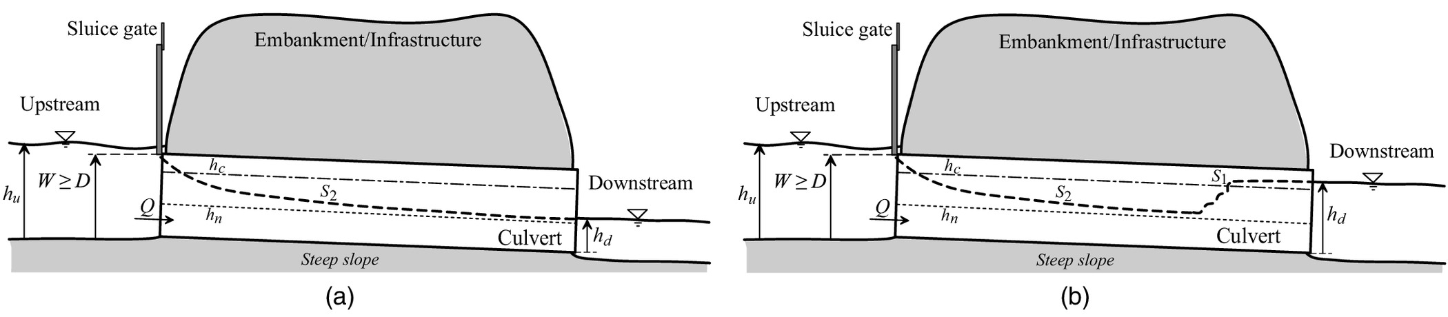
Consider a steady discharge through a gated circular culvert with a flat-bottomed sluice gate of opening ; culvert slope, diameter and length, , , and , respectively; and upstream and downstream flow levels above the culvert invert ends and , respectively, where [Fig. 1(b)]. A circular cross-section was selected because it is the most common section for culverts. However, other cross-sectional shapes could be considered by replacing with the corresponding characteristic length. The multiple steady flow states inside the culvert can be analyzed based on the gradually varied flow theory in combination with control-volume momentum conservation for positioning hydraulic jumps. The flow solutions are determined by identifying the relative position of the critical and normal flow depths inside the culvert, and , respectively. The hydraulic operation is classified according to the location of the control section (Normann et al. 1985; Chaudhry 2008; Schall et al. 2012), defined as a section in which there is a unique relationship between the flow rate and the flow depth (Normann et al. 1985; Schall et al. 2012). When the discharge depends only on the approach flow conditions, the control section is at the inlet (inlet control). In contrast, when the discharge is governed by a combination of the culvert geometry and resistance to flow, inlet, and outlet conditions, the control is at the outlet section (outlet control). The nomenclature chosen to analyze and group the different steady flow states likely to be formed in gated circular culverts is as follows: inlet and outlet control states are named and , respectively, where is the group of flow cases sharing characteristics (= ).

Inlet Control Classification
Inlet control flows often are characterized by the presence of supercritical flow within the culvert. In gated culverts, the main features affecting inlet control flow operations are: (1) inlet flow level, (2) sluice gate opening, (3) geometrical characteristics of the culvert determining the flow area, and (4) inlet elements for flow contraction used to accelerate the flow from the approach channel to the tube flow within the circular culvert, such as walls and/or wings (Normann et al. 1985; Schall et al. 2012). The flow at the inlet control section can be free or submerged. For inlet flow levels implying no culvert-entrance submergence, i.e., (Chaudhry 2008), the flow entrance works similarly to a weir crest flow, with critical flow occurring just downstream from the tube entrance and gate. Flow from the inlet gate to the critical depth section involves high streamline curvature effects, a feature not accounted for in the present flow profile classification but occurring only in a short portion of the tube, close to the gate. When the gate is fully open () and the inlet flow levels involve culvert-entrance submergence, i.e., (Chaudhry 2008), hydraulically the entrance works as an orifice. These theoretical limits apply for dominating inlet head-losses and, thus, with negligible friction head losses within the culvert, which normally is the scenario in hydraulically short pipes. For hydraulically long culverts, the wall-dominated friction head losses within the culvert are significant, and, thus, the flow cases become outlet control. Generally, conditions corresponding to imply pressurized flow from the inlet section (Chaudhry 2008), so these conditions fall into outlet control.
However, to be precise, under flow submergence conditions and partial gate opening (), the flow is governed by the hydraulics of a more complex orifice shape formed by the combined shape of the pipe inlet and the gate (Fan 1985), hereon denoted flow under a sluice gate for practical purposes. The aforementioned theoretical limits for flow classification criteria appear as being adjusted below, according to the experiments in this work (see details in Appendix I). The subsequent steady flow states, which depend on the inlet and outlet submergences, are analyzed in the following subsections. Approach velocity effects were not considered in the ensuing discussion. In the plots, contraction effects past the sluice gate are not represented graphically.
I1: Inlet and Outlet Free-Surface Flow (Fig. 2)
If , , and the outlet flow depth is less than the critical depth, , there is supercritical flow along the culvert. The flow solution is determined by the slope of the culvert and the position of relative to and . Depending on its slope, four jump-free steady flow states can be developed in the culvert [Figs. 2(a–d)]. The theoretical steady flow state in Fig. 2(d) may occur rarely in practice unless a steep reach leads to the entrance, thus ensuring supercritical flow upstream of the control section.

If , a subcritical flow on the upstream side of the culvert downstream end occurs, and hence provides the conditions for the development of a hydraulic jump [Figs. 2(e–f)].
Flow characteristics and condition details of the steady flow cases in Fig. 2 are summarized in Table 1 (Appendix I).
| Reference | Flow conditions at both ends | Culvert slope | Comments |
|---|---|---|---|
| Fig. 2(a) | Steep | The flow depth at the control section is . The flow downstream of the control section is supercritical and described by an -type curve. | |
| Fig. 2(b) | The flow depth at the control section is . The flow downstream of the control section is supercritical and described by an -type curve. | ||
| Fig. 2(c) | The flow depth at the control section is . The flow downstream of the control section is supercritical and asymptotic to as described by an -type curve. | ||
| Fig. 2(d) | Mild | The control section is upstream of the culvert entrance. The flow depth depends on the inlet elements and the channel geometry. The supercritical flow inside the culvert is described by an -type curve. | |
| Fig. 2(e) | Steep | The flow depth at the control section is . The flow downstream of the inlet section is divided into three zones: (1) -type curve downstream of the control section, (2) -type curve upstream of the outlet section, and (3) a hydraulic jump as transition. | |
| Fig. 2(f) | Mild | The flow depth at the control section is . The flow downstream of the inlet section is divided into three zones: (1) -type curve downstream of the control section, (2) -type curve upstream of the outlet section, and (3) a hydraulic jump as transition. | |
I2: Inlet Free Surface and Outlet Submerged Flow (Fig. 3)
If , , and the outlet flow depth is greater than the culvert diameter, , which indicates submergence at the culvert downstream end, the flow in the culvert includes: (1) supercritical flow downstream from the inlet section; (2) subcritical flow upstream of the outlet section, rendering a partly pressurized culvert; and (3) a hydraulic jump within the culvert. These steady-flow states usually are achieved under steep slope conditions [Fig. 3 and Table 2 (Appendix I)].

| Reference | Flow conditions at both ends | Culvert slope | Comments |
|---|---|---|---|
| Fig. 3 | Steep | The flow depth at the control section is . The flow downstream of the inlet section is divided into three zones: (1) -type curve downstream of the control section, (2) subcritical flow pressurized upstream of the outlet section, and (3) a hydraulic jump as transition. | |
I3: Inlet Submerged and Outlet Free-Surface Flow (Figs. 4 and 5)
If and , or and , and , the culvert entrance is submerged and the flow inside the culvert is developed under supercritical, free-surface conditions. In this inlet control group, the position of the gate determines the type of flow. That is, if , an orifice-type flow, the shape of which is determined by the pipe inlet, is expected. Fig. 4 and Table 3 (Appendix I) present these flow conditions (with and without hydraulic jumps), which are subjected to steep slope conditions. Between the inlet and the critical depth sections, the flow varies rapidly; therefore the plot of this portion of the flow profile in Fig. 4 is only approximate. However, under mild or horizontal slope conditions, the flow is expected to switch from inlet to outlet control conditions if .

| Reference | Flow conditions at both ends | Culvert slope | Comments |
|---|---|---|---|
| Fig. 4(a) | Steep | The control section is slightly displaced downstream of the orifice inlet due to flow contraction effects in the inlet section. The flow is divided into two zones: (1) transition curve typical after orifices until is reached, and (2) -type curve until . | |
| Fig. 4(b) | The control section is slightly displaced downstream of the orifice inlet due to flow contraction effects at the inlet section. The flow is divided into four zones: (1) transition curve typical after orifices until is reached, (2) -type curve downstream of the control section, (3) -type curve upstream of the culvert outlet, and (4) a hydraulic jump as transition. | ||
| Fig. 5(a) | The control section is slightly displaced downstream of the sluice gate due to flow contraction effects at the inlet section. The flow is divided into two zones: (1) transition curve typical after orifices until is reached, and (2) -type curve until . | ||
| Fig. 5(b) | The control section is at the sluice gate. The flow downstream of the control section is supercritical and described by an -type curve until . | ||
| Fig. 5(c) | The control section is at the sluice gate. The flow downstream of the control section is supercritical and described by an -type curve until . | ||
| Fig. 5(d) | Mild | The control section is at the sluice gate. The flow downstream of the control section is supercritical, fast contracted. After that, it is described by a -type curve until . | |
| Fig. 5(e) | Steep | The control section is slightly displaced downstream of the sluice gate due to flow contraction effects at the inlet section. The flow is divided into three zones: four zones: (1) transition curve typical after orifices until is reached, (2) -type curve downstream of the control section, (3) -type curve upstream of the culvert outlet, and (4) a hydraulic jump as transition. | |
| Fig. 5(f) | The control section is at the sluice gate. The flow is divided into three zones: (1) -type curve downstream of the control section, (2) -type curve upstream of the culvert outlet, and (3) a hydraulic jump as transition. | ||
| Fig. 5(g) | The control section is at the sluice gate. The flow is divided into three zones: (1) -type curve downstream of the control section, (2) -type curve upstream of the culvert outlet, and (3) a hydraulic jump as transition. | ||
| Fig. 5(h) | Mild | The control section is at the sluice gate. The flow is divided into four zones: (1) fast contraction of flow after the sluice gate, (2) -type curve downstream of the end of the contracted flow, (3) -type curve upstream of the culvert outlet, and (4) a hydraulic jump as transition. | |
I4: Inlet and Outlet Submerged, with Free-Surface Flow between (Fig. 6)
If with , or but , the culvert inlet is considered to be submerged. If the culvert outlet also is submerged (), there must be a transition from supercritical to subcritical flow with a hydraulic jump. Similarly to the I3 group, the position of the sluice gate determines the type of flow. If , orifice-type flow takes place, although the transition to supercritical flow is expected with steep slopes [Fig. 6(a) and Table 4 in Appendix I], whereas a mild slope switches to outlet control. If , the expected flow under the sluice gate types are as depicted in Figs. 6(b–e) and described in Table 4 (Appendix I). Near the critical depth, flow profiles are rapidly-varied, as previously explained.

| Reference | Flow conditions at both ends | Culvert slope | Comments |
|---|---|---|---|
| Fig. 6(a) | Steep | The control section is slightly displaced downstream of the orifice inlet due to flow contraction effects in the inlet section. The flow is divided into three zones: (1) transition curve typical after orifices until is reached, (2) -type curve, and (3) a hydraulic jump from supercritical free-surface flow to subcritical pressurized flow. | |
| Fig. 6(b) | The control section is slightly displaced downstream of the sluice gate due to flow contraction effects in the inlet section. The flow is divided into three zones: (1) transition curve until is reached, (2) -type curve, and (3) a hydraulic jump from supercritical free-surface flow to subcritical pressurized flow. | ||
| Fig. 6(c) | The control section is at the sluice gate. The flow is divided into two zones: (1) -type curve, and (2) a hydraulic jump from supercritical free-surface flow to subcritical pressurized flow. | ||
| Fig. 6(d) | The control section is at the sluice gate. The flow is divided into two zones: (1) -type curve, and (2) a hydraulic jump from supercritical free-surface flow to subcritical pressurized flow. | ||
| Fig. 6(e) | Mild | The control section is at the sluice gate. The flow is divided into three zones: (1) fast contraction of flow after the sluice gate, (2) -type curve downstream of the end of the contracted flow, and (3) a hydraulic jump from supercritical free-surface flow to subcritical pressurized flow. | |
Outlet Control Classification
For outlet control, the steady flow may involve a pressurized flow in combination with subcritical free-surface flow profiles, thus without a hydraulic jump formation. In gated culverts, the main features influencing the outlet control flow are: (1) the cross-sectional culvert area, (2) the shape of the culvert cross section, (3) the length of the culvert, (4) the flow resistance in the culvert, and (5) the flow depths at both culvert invert ends (Normann et al. 1985; Chaudhry 2008; Schall et al. 2012). For cases not implying submergence of the culvert outlet, the flow depth at the control section is . If the tailwater level is below , there is a critical depth control located upstream within the culvert. For , the flow conditions are subcritical (tranquil) along the culvert, and there is no occurrence of the critical depth in any section (Schall et al. 2012; Chin 2013). The sluice gate action, as depicted for the inlet control flow states, affects the submergence conditions at the inlet, and, therefore, the hydraulic flow solution along the culvert. In the following subsections, outlet control steady flow cases are arranged in five major groups, in which the theoretical limits for the boundary variables have been adjusted based on experimental results when pertinent (Appendix I).
O1: Inlet Free Surface and Outlet Submerged Flow (Fig. 7)
If the inlet flow depth satisfies the condition , with for steep slopes or for mild slopes, and the outlet is submerged, i.e., , two flow zones can be distinguished in the culvert: (1) subcritical free-surface flow just downstream from the inlet, followed by (2) pressurized flow to the outlet section. The possible flow states depend on the culvert slope [Fig. 7 and Table 5 (Appendix I)]. For gate openings involving or for steep and mild slopes, respectively, the flow switches to inlet control [Figs. 6(c and e), respectively].

| Reference | Flow conditions at both ends | Culvert slope | Comments |
|---|---|---|---|
| Fig. 7(a) | Steep | The flow is divided into three zones: (1) transition curve upstream of the culvert from until , (2) -type curve downstream of the sluice gate to reach a point of pressurization, and (3) pressurized flow until the control section. | |
| Fig. 7(b) | The flow is divided into two zones: (1) free surface profile downstream of the sluice gate described by an -type curve to reach a point of pressurization, and (2) pressurized flow until the control section. | ||
| Fig. 7(c) | Mild | The flow is divided into three zones: (1) transition curve upstream of the culvert from until , (2) -type curve downstream of the sluice gate to reach a point of pressurization, and (3) pressurized flow until the control section. | |
| Fig. 7(d) | The flow is divided into two zones: (1) free surface profile downstream of the sluice gate described by a -type curve to reach a point of pressurization, and (2) pressurized flow until the control section. | ||
O2: Inlet and Outlet Submerged Flow with Fully Pressurized Culvert (Fig. 8)
If and , with the outlet flow depth , there is fully pressurized flow in the culvert regardless of the bottom slope (Fig. 8 and Table 6 in Appendix I).

| Reference | Flow conditions at both ends | Culvert slope | Comments |
|---|---|---|---|
| Fig. 8 | — | The flow is fully pressurized along the culvert. | |
O3: Inlet Free Surface or Submerged and Outlet at Full Culvert Flow (Fig. 9)
For , partly or fully pressurized flow can be developed within the culvert. Depending on both and the position of the gate, the flow at the inlet results in (1) free-surface flow with a transition to pressurized flow if and [Figs. 9(a and c) for steep and mild slopes, respectively] or (2) submerged sluice gate upstream with likely free-surface flow behind if and [Figs. 9(b and d) for steep and mild slopes, respectively]. The details of the flow states allowing free-surface flow after the inlet section, which depend on the slope of the culvert, are given in Table 7 (Appendix I).

| Reference | Flow conditions at both ends | Culvert slope | Comments |
|---|---|---|---|
| Fig. 9(a) | Steep | The flow is divided into three zones: (1) transition curve upstream of the culvert from until , (2) -type curve downstream of the sluice gate to reach a point of pressurization, and (3) pressurized flow until the control section at full culvert. | |
| Fig. 9(b) | The flow is divided into two zones: (1) free surface profile downstream of the sluice gate described by an -type curve to reach a point of pressurization (likely if ), and (2) pressurized flow until the control section at full culvert. | ||
| Fig. 9(c) | Mild | The flow is divided into three zones: (1) transition curve upstream of the culvert from until , (2) -type curve downstream of the sluice gate to reach a point of pressurization, and (3) pressurized flow until the control section at full culvert. | |
| Fig. 9(d) | The flow is divided into two zones: (1) free surface profile downstream of the sluice gate described by a -type curve to reach a point of pressurization (likely if ), and (2) pressurized flow until the control section at full culvert. | ||
O4: Inlet Submerged and Outlet Free-Surface Flow with Partly Pressurized Culvert (Fig. 10)
If and the outlet flow depth is greater than, or equal to, the critical depth, i.e., , a free-surface profile develops from in the upstream direction until the culvert flow becomes pressurized elsewhere, resulting in a fully submerged culvert inlet section. The subsequent flow cases, which depend on the slope of the culvert, are described in Fig. 10 and Table 8 (Appendix I).

| Reference | Flow conditions at both ends | Culvert slope | Comments |
|---|---|---|---|
| Fig. 10(a) | Horizontal | The flow is divided into two zones: (1) pressurized flow until the point of separation, and (2) -type curve until . | |
| (in practice, i.e., for modeling) | |||
| Fig. 10(b) | Mild | The flow is divided into two zones: (1) pressurized flow until the point of separation, and (2) -type curve until . | |
O5: Inlet and Outlet Free-Surface Flow (Fig. 11)
If and the outlet flow depth is generally for both steep and mild slope conditions, the flow is subcritical in the entire culvert imposing . The subsequent flow cases, which depend on the culvert’s slope and the submergence of the entrance, are described in Fig. 11 and Table 9 (Appendix I). Tranquil flow, i.e., with no gate action, is plotted in Fig. 11(a).

| Reference | Flow conditions at both ends | Culvert slope | Comments |
|---|---|---|---|
| Fig. 11(a) | Mild | The flow solution is described by an -type curve until . | |
| Fig. 11(b) | |||
| Fig. 11(c) | Mild | The flow solution is described by an -type curve until . | |
| Fig. 11(d) | |||
| Fig. 11(e) | Mild | The flow solution is described by an -type curve until in the control section. | |
| Fig. 11(f) | |||
| Fig. 11(g) | Steep | The flow solution is described by an -type curve until . | |
| Fig. 11(h) | |||
Fig. 12 summarizes the flow classification scheme described above using decision trees for inlet and outlet control.

Laboratory Experiments
A laboratory investigation was conducted at the hydraulic facilities of the Institut Agro, Montpellier (France). A gated circular culvert made of polymethyl methacrylate (PMMA), i.e., transparent acrylic, for both the pipe and gate was installed in a prismatic, tilting flume 7 m long, 0.29 m wide, and 0.5 m high (Figs. 13 and 14). The circular culvert was 0.15 m in diameter and 2 m long. This is about half the size of typical outlet structures in rice irrigation schemes in southern Spain. The sluice gate consisted of a square PMMA plate fixed with clamps to the wall of the flume and operated manually. The pipe was installed 3 m downstream from the flume inlet, leaving a distance of 2 m from the pipe end to the flume tailgate. The experimental setup included eight Baumer U500.DA0-AA1B.720 ultrasonic sensors (Frauenfeld, Switzerland), operated at a frequency of 30 Hz, to measure flow levels at four points upstream from the entrance of the pipe and four points downstream from the exit. The sensors were installed using a rack that maintained an interval distance of 0.16 m between each; the sensors closest to the upstream and downstream pipe ends were 0.04 m from the inlet and outlet culvert sections (the minimum distance required according to the technical specifications). The discharge was measured using an electromagnetic flowmeter (Krohne WATERFLUX 3100 C; discharge range , accuracy 99.7%, Duisburg, Germany) installed in the flume recirculation pipe. Pressure and water level inside the culvert pipe were measured using 15 piezometers installed equidistant on the bottom edge of the culvert pipe along the first 1.2 m of the inlet. The piezometers were read manually with an approximate uncertainty of in the presence of hydraulic jumps when the fluctuating pressure was averaged; otherwise the estimated uncertainty diminished to approximately , i.e., for steady flow cases without a hydraulic jump.

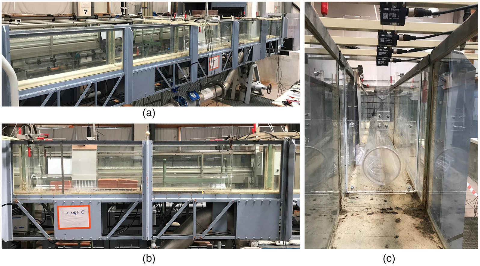
The experimental setup permitted five groups of conditions to be established, namely I3 for inlet control, and O2, O3, O4, and O5 for outlet control. Other groups, most of them associated with steep slope conditions, could not be generated in the flume because the inlet and outlet walls of the culvert were fixed perpendicularly to the flume direction (Fig. 14), so that the high slopes would not resemble real conditions in which the inlet and outlet walls are vertical. Photographs of the laboratory observation of the control groups explored are provided in Fig. 15. A total of 230 tests were conducted: 190 with , 22 with , and 18 with . The case of corresponded to the residual slope of the flume at its horizontal position. In terms of the reproducibility of the tests for scientific purposes, we have maintained this value in the manuscript rather than horizontal () given that the level is sensitive to and is relevant to the classification of steady flow solutions. Each test lasted at least 10 min, the time to reach steady flow conditions. All Reynolds numbers were in the interval . The data set is given in Appendix II.

Results
Findings for the application of the proposed gated circular culvert flow classification scheme to the new laboratory database are presented in this section. The scheme proposed in this work comprised 41 steady flow cases organized into 4 inlet control and 5 outlet control groups, which exceeds the classification groups by other existing gated culvert flow classifications, e.g., that by Fan (1985). Prior to the evaluation of data using our scheme, we compared our proposed scheme with the flow classification scheme by Fan (1985) to check whether the grouping into common flow conditions types was preserved. For that purpose, full pipe and orifice flow types by Fan (1985) were selected. These were identified with our proposed O2 and I3 groups, respectively. According to Fan (1985), the classification criteria are or with for full pipe flow, and or with for orifice flow. The experimental tests classified as full pipe flow by Fan’s (1985) scheme coincided with those classified by our scheme as O2 group. However, when classifying orifice flow types using Fan’s (1985) scheme, not only were tests pertaining to the I3 group detected but also those of the O4 group, e.g., Experiments 170, 173, and 176. This indicates that our classification scheme can be regarded as offering a more-detailed classification of steady flow cases than others available for gated circular culverts. Correspondence between the proposed and previous classifications is provided in Appendix III, along with available discharge equations associated with each flow condition.
Relationship between Discharge and Flow Variables
A general relationship between the discharge and the flow and geometry variables for flow through gated circular culverts can be written as follows:where = Manning roughness coefficient; = dynamic viscosity; = flow density; and = gravitational acceleration. For the analysis of our data, constant variables during experimentation were dropped in Eq. (1), resulting in
(1)
(2)
The relevant variables in Eq. (2) are , , and for inlet control, and , , and for outlet control. is an operational variable, whereas is a design variable, and therefore both are fixed. Then discharge can be represented versus for inlet control data analysis and versus for outlet control data analysis, while keeping and constant. The datum reference level for outlet control is set at the culvert exit, so the upstream water level is . Rating equations were derived from Eq. (2) for inlet and outlet control conditions.
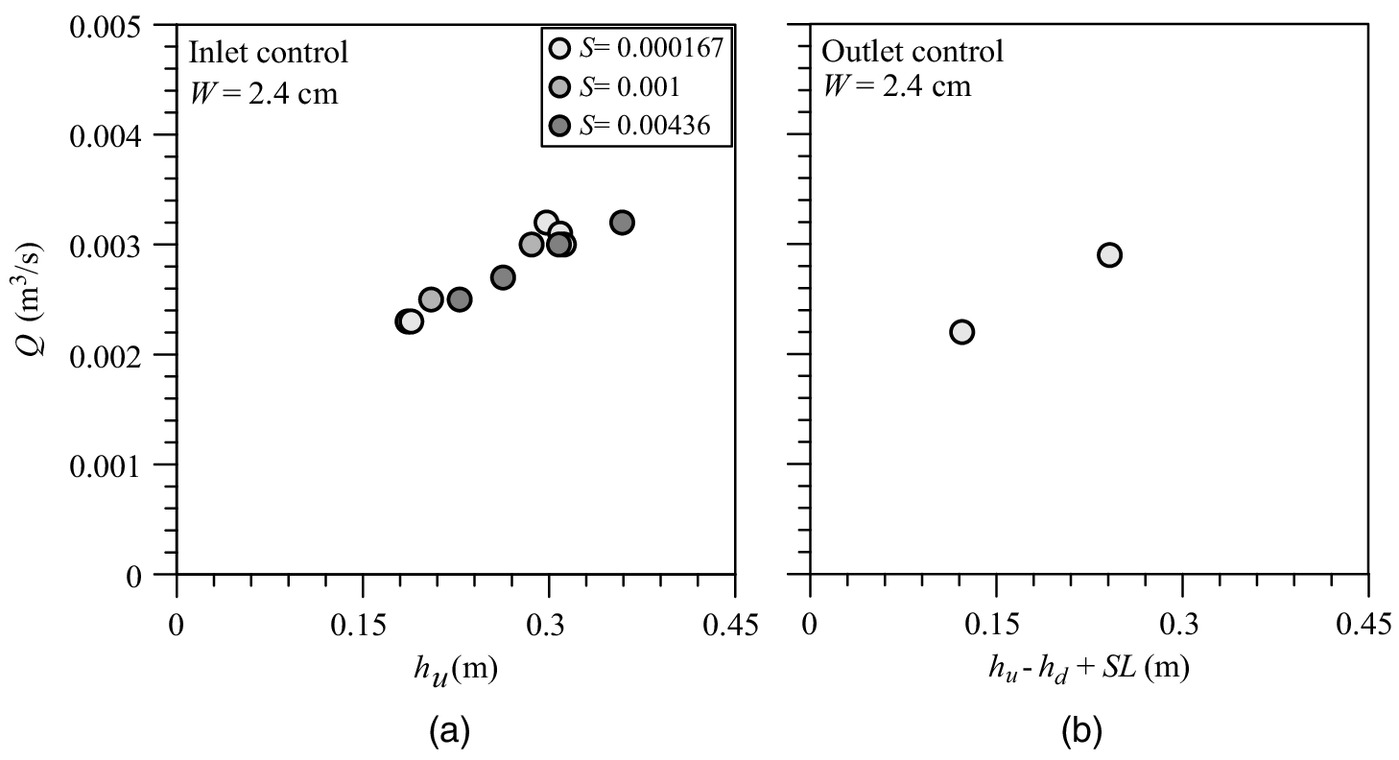
Figs. 16(a, c, and e) show the inlet-control data in versus charts for , 0.001, and 0.00436, respectively. Similarly, Figs. 16(b, d, and f) show the outlet-control data in versus charts for the same slopes. Data not affected by the gate () also are plotted in Fig. 16(b). The data in the charts are arranged by groups with similar . Discharge data with similar depicts trends followingwhere and = scaling and exponent parameters, respectively, depending on and ; and = head given by for inlet control and for outlet control. In each case, rating parameters include all effects, whether or not friction head losses are significant, considering that both local and friction head losses are related to kinetic energy. However, hydraulically long culverts may have very different flow profiles, e.g., due to the presence (or absence) and location of a hydraulic jump within the pipe, and the variability of the wetted area within the pipe. Because the evaluation of all head losses in the tests was beyond the scope of this study, specific rating curves for hydraulically long tests were not adjusted here, but are included in the data set for outlet control. The discharge rating analysis conducted is shown in Figs. 16 and 17 for the inlet and outlet control groups, respectively, using Eq. (3). The and values in Figs. 16 and 17 were determined by the best power fit of the data as grouped by narrow ranges of . The average of each range is labeled in Figs. 16 and 17 over each corresponding rating curve. As expected for the operation of an orifice-controlled flow, was in the range 0–1, with typical values around 0.5 for inlet control [Figs. 16(a, c, and e)]. Thus the latter applies to hydraulically short culverts. In addition, data were found to be directly proportional to the gate opening, i.e., large produced flows that exceeded those of small , with an evident direct dependency of and on for each values. This arrangement was clear for inlet control, for which all data points corresponded to a single flow state, I3, with with , and with , for . However, the outlet-control data points corresponded to four different flow states (O2, O3, O4, and O5), so that the different groups overlapped, especially for . These flow cases describe situations for which the gate may exert little control on the flow, with the outlet and culvert friction head-losses becoming significant, as in hydraulically long culverts. Only if the frictional head-losses within the culvert become significant, should an addend appear on the right-hand side of Eq. (3) (Zeng et al. 2020). Fig. 17 shows the data points in Fig. 16(b) as separated by outlet control states, as well as their rating analysis using Eq. (3). The arrangement of data points by then becomes evident in the domain , whereas overlapping remains in the region near the origin, namely when . In Fig. 17, data with no gate action for O4 and O5 groups are not analyzed by means of Eq. (3) because they show overlapping with gate action data, and so do the resulting rating curves. This rating analysis was not intended to provide a modeling tool, but just to discuss the results and arrangement of data.
(3)


Using Eq. (3), flow transition regions in the discharge rating, i.e., between data pertaining to different groups of conditions, can be discussed. Exploring all 41 steady flow cases in Figs. 2–11, the main flow transition regions identified between groups were: (1) I1 to I3, (2) I2 to I4, (3) O1 to O2, and (4) O5 to I3. Other likely transitions between flow cases or groups are not accounted for here. Due to the lack of data for groups I1, I2, I4, and O1 in this work, flow transition regions in Transition regions 1–3 could not be analyzed. However, these transitions can be analyzed theoretically. For example, as increases in Transition region 3, the flow states evolve describing a reduction of the length of the likely developed -type curve in the O1 group leading to fully pressurize culvert in the O2 group. However, the occurrence of Transition region 4 was confirmed by conducting an experiment in which the discharge was increased progressively by maintaining all other conditions in the flume and gated circular culvert model. Fig. 18 shows the analysis of the flow transitions zones between the O5 outlet and I3 inlet groups for main gate openings of 8.75 and 6.25 cm. To compare both type of rating curves, the -axis of the O5 curves was scaled using the observed averaged ratios: 0.53 for , and 0.47 for . Thereby, the head in the outlet discharge rating curves [Eq. (3)], which is , was approximated as for and as for , neglecting the term. Thus, the -axis in the O5 curves originally plotted in Fig. 17 was converted into and for 8.75- and 6.25-cm gate openings, respectively. Snapshots of the video recorded for the discharge incrementing experiment that motivated this analysis also are shown in Fig. 18, in which the transition from O5 outlet control conditions to I3 inlet control conditions is evident in time. According to Bodhaine (1968), straight lines can be used to connect two rating curves. We propose parabolic transitions to maintain continuity between curves. However, more experimental data are required to help define these flow transition regions accurately. This gains importance at low stages if critical flow may occur upstream from the culvert inlet section, i.e., in the approach flow, and at stages in which high head flow is likely to occur (Bodhaine 1968).

Fig. 19 depicts the influence of on the versus head relationship. Inlet and outlet control data for (the most numerous subgroups of data including the maximum of values of in both the inlet and outlet control tests) are displayed in Figs. 19(a and b), respectively; the three different values of tested are indicated by different shades. With the selected gate opening, no differences were observed in the versus head relationship due to the variation in in the interval of tested at both groups. Thus, the influence of on the versus head relationship is unclear in the range of tested in our experiments.
Empirical Discharge Rating of Gated Culverts
The preceding results reveal the complexity of the hydraulics within gated culverts. Such complexity could be tackled empirically using dimensionless models like the one proposed by Zeng et al. (2020). That model relies on four dimensionless flow rating equations for gated culverts to model different flow conditions groups, namely (1) mild slope culvert orifice or full pipe flow, (2) mild slope culvert open channel flow, (3) steep-slope culvert full pipe flow, and (4) steep slope culvert unsubmerged or submerged with inlet control, which are, respectivelywhere ; and = cross-sectional flow area beneath gate and , respectively; = cross-sectional area of culvert; and , , = empirical parameters. Eqs. (4)–(7) relate the dimensionless head to the dimensionless discharge by means of three empirical, case-dependent parameters. Whereas Eqs. (4) and (5) are derived for mild slopes (i.e., ) with and , respectively, Eqs. (6) and (7) apply for steep slopes (i.e., ) with and , respectively (Zeng et al. 2020). According to Zeng et al. (2020), accounts for the roughness effect; thus, for the experiments in this study, it was assumed that , which is consistent for short barrels with negligible friction losses. Calibrating and for the data collected in the present experiments, Figs. 20(a and b) show the performance of Eq. (4) for our experimental data in the Zeng et al.’s (2020) subgroup “mild slope culvert orifice or full pipe flow.” The combination of , , and produced the best fit, with errors in the prediction of the dimensionless discharge bounded by and limits [Fig. 20(b)]; was set equal to 2 in Fig. 20(a) to maintain the energy balance analogy with Eq. (4), which is an appropriate value for outlet control flow (Zeng et al. 2020). Figs. 20(c and d) depict the application of Eq. (5) to our data in the subgroup “mild slope culvert open channel flow.” The best fit was found using , , and , which had modeling errors bounded by and limits [Fig. 20(d)]. Lastly, the results of applying Eq. (7) to our data in the subgroup “steep slope culvert unsubmerged or submerged with inlet control” are shown in Figs. 20(e and f). Here, the combination of , , and led to the best fit, with estimation errors within limits [Fig. 20(f)]. Eq. (6) could not be tested here because none of our data satisfied the criteria of Zeng et al.’s (2020) subgroup “steep-slope culvert full pipe flow.” Numerical tests with Eqs. (4), (5), and (7) showed that the uncertainty of level measurements (which was very little in our experiments) could explain only a very small part of the error in predictions. According to Zeng et al. (2020), the discharge coefficient for a flow under a sluice gate in inlet control conditions is an independent variable for in Eq. (7). Considering the results in Figs. 20(e and f), this suggests that should not be approximated by a single value for a group of data, but its modeling is rather complex and deserves further investigation. This issue also occurred in the analysis of errors by Eqs. (4) and (5), given that the scaling parameter is defined as , where is the discharge coefficient expressing contraction associated with culvert entrance edge and gate conditions (Zeng et al. 2020). Eqs. (4) and (5) are case-dependent, and thus require site-specific calibration.
(4)
(5)
(6)
(7)

Conclusions
This work proposes an inlet–outlet control–based classification of steady flow through gated circular culverts. A total of 22 inlet control states and 19 outlet control states were organized into groups of operational conditions, revealing the complexity of the flow through this type of hydraulic structure. Four groups for inlet control (I1, I2, I3, and I4) and five groups for outlet control (O1, O2, O3, O4, and O5) were identified as sharing flow conditions. Rapidly varied flow transitions through critical depth at the inlet and/or outlet were not studied in detail, e.g., for rating analysis. They were considered only as part of the steady flow states by this classification scheme. Based on the proposed classification scheme, 230 laboratory tests were carried out to relate discharge through the culvert of the opening to the gate , the slope of the culvert , and the up- and downstream water depths. The laboratory setup allowed exploration of one inlet control (I3) and four outlet control groups (O2, O3, O4, and O5) of conditions. Most of the groups determined by steep slopes could not be explored due to the experimental setup constraints, which poses a limitation of the study. Comparison with the existing flow classification scheme for gated culverts by Fan (1985) indicated that the proposed scheme in this work is able to classify flow into more subtypes, i.e., with more detail, which can be regarded as an advantage for future research on discharge rating. This is the case of flow states with a hydraulic jump under gate action, the computation and location of which are key to determining control type and, therefore, to developing accurate discharge rating equations. This task could be carried out in a rigorous manner using the proposed classification scheme on gated culvert flow and the detailed flow descriptions provided here.
Because they were organized by narrow ranges of gate openings, the data were found to depict a power relationship with head data, following Eq. (3), with exponents between 0 and 1, which is in line with traditional discharge-rate expressions for orifice-controlled flow. Hydraulically long tests were included in the outlet control data for analysis. The use of Eq. (3) for those situations should be regarded as an approximation because head losses were not accounted for. For some outlet-control group flow cases, Eq. (3) could not be used due to data overlapping, thus indicating that exponent values between 0 and 1 may be applicable only to hydraulically short culverts. Inspecting the influence of the independent variables indicated that the gate opening had the greatest effect on the discharge, exhibiting a direct proportional relation. Flow transition regions also were analyzed, focusing on the transition between O5 and I3 groups which was evidenced during the experimental work. Parabolic curves are proposed for these regions of transition, although more data are required to clarify the connection between curves. To explore all the theoretical flow cases, future research should address the limitations posed by the present experimental setup, testing different lengths of the barrel, testing different materials (i.e., roughness), allowing for visual inspection, and testing steep slopes consistent with real conditions, in which inlet and outlet walls are vertical.
The experiments were analyzed using the empirical model proposed by Zeng et al. (2020). By adjusting its parameters, it was possible to predict the discharge within an error band of for inlet control and to for outlet control. However, the discharge equations derived are case-dependent, requiring accurate experimental data for calibration. A hydraulic model with capabilities to predict free-surface and pressurized flows within culverts would represent an alternative and/or complementary tool, and will be the scope of future research. For this purpose, the application of the proposed gated circular culvert flow classification scheme will be essential.
Notation
The following symbols are used in this paper:
- cross-sectional area of culvert;
- cross-sectional flow area beneath gate;
- cross-sectional flow area beneath ;
- discharge coefficient expressing contraction associated with culvert entrance edge and gate conditions;
- discharge coefficient;
- , ,
- empirical parameters;
- circular culvert diameter;
- ;
- gravitational acceleration;
- flow head;
- critical depth;
- downstream flow level above outlet culvert invert end;
- culvert friction losses;
- normal depth;
- upstream flow level above inlet culvert invert end;
- culvert length;
- Manning roughness coefficient;
- discharge;
- coefficient of determination;
- Reynolds number;
- culvert slope;
- gate opening;
- group of flow cases sharing characteristics (= 1, 2, …, 5);
- scaling parameter;
- exponent parameter;
- flow density; and
- dynamic viscosity.
Appendix I. Classification Details by Groups of Conditions
Tables 1–9 summarize conditions for the inlet control groups I1–I4 and the outlet control groups O1–O5, respectively. The standard nomenclature for classifying gradually varied flow free-surface curves is used here to describe further each flow case, namely , , and types for steep slopes (); , , and types for mild slopes (); and type for horizontal slopes () (Montes 1998; Castro-Orgaz and Hager 2019). A horizontal culvert is considered to be a limit case of mild slope, with (in this case, an -type backwater curve does not exist; Fig. 10 provides an example of this). A detailed description of gradually-varied flow profiles was given by Castro-Orgaz and Hager (2019).
Appendix II. Experimental Database
Experimental data are presented in Table 10, including the discharge and geometric characteristics for the operational conditions in each experiment. Piezometer measurements in experiments 1−150 are not presented for the sake of brevity.
| Experiment | () | (mm) | (mm) | (mm) | (mm) | Group of conditions | Theoretical case | |
|---|---|---|---|---|---|---|---|---|
| 1 | 2.9 | 160 | 81 | 44 | 150 | 0.000167 | O5 | Fig. 11(e) |
| 2 | 1.9 | 160 | 66.5 | 38 | 150 | 0.000167 | O5 | Fig. 11(e) |
| 3 | 1.5 | 160 | 59 | 33 | 150 | 0.000167 | O5 | Fig. 11(e) |
| 4 | 1 | 160 | 52 | 29 | 150 | 0.000167 | O5 | Fig. 11(c) |
| 5 | 2.5 | 38 | 98 | 46 | 150 | 0.000167 | I3 | Fig. 5(h) |
| 6 | 3.8 | 38 | 164 | 47 | 150 | 0.000167 | I3 | Fig. 5(d) |
| 7 | 4.2 | 38 | 194 | 95 | 150 | 0.000167 | I3 | Fig. 5(h) |
| 8 | 5.2 | 38 | 265 | 113 | 150 | 0.000167 | I3 | Fig. 5(h) |
| 9 | 5.7 | 38 | 308 | 125 | 150 | 0.000167 | I3 | Fig. 5(h) |
| 10 | 5.5 | 38 | 317 | 44 | 150 | 0.000167 | I3 | Fig. 5(d) |
| 11 | 5.5 | 38 | 312 | 113 | 150 | 0.000167 | I3 | Fig. 5(h) |
| 12 | 2.6 | 20 | 295 | 89 | 150 | 0.000167 | I3 | Fig. 5(h) |
| 13 | 2.6 | 20 | 293 | 52 | 150 | 0.000167 | I3 | Fig. 5(h) |
| 14 | 3 | 20 | 375 | 101 | 150 | 0.000167 | I3 | Fig. 5(h) |
| 15 | 11.5 | 72 | 278 | 74 | 150 | 0.000167 | I3 | Fig. 5(d) |
| 16 | 14.1 | 72 | 339 | 94 | 150 | 0.000167 | O4 | Fig. 10(b) |
| 17 | 13.5 | 72 | 372 | 74 | 150 | 0.000167 | I3 | Fig. 5(d) |
| 18 | 20.3 | 106.5 | 285 | 139 | 150 | 0.000167 | O3 | Fig. 9(d) |
| 19 | 7.1 | 106.5 | 136 | 106 | 150 | 0.000167 | O5 | Fig. 11(d) |
| 20 | 12.4 | 106.5 | 190 | 124 | 150 | 0.000167 | O4 | Fig. 10(b) |
| 21 | 17.1 | 106.5 | 248 | 134 | 150 | 0.000167 | O3 | Fig. 9(d) |
| 22 | 21.6 | 106.5 | 365 | 179 | 150 | 0.000167 | O2 | Fig. 8 |
| 23 | 17.1 | 106.5 | 362 | 248 | 150 | 0.000167 | O2 | Fig. 8 |
| 24 | 10.3 | 134 | 156 | 101 | 150 | 0.000167 | O5 | Fig. 11(d) |
| 25 | 7.4 | 134 | 129 | 88 | 150 | 0.000167 | O5 | Fig. 11(c) |
| 26 | 16.8 | 134 | 217 | 139 | 150 | 0.000167 | O4 | Fig. 10(b) |
| 27 | 17.7 | 134 | 310 | 214 | 150 | 0.000167 | O2 | Fig. 8 |
| 28 | 2.3 | 24 | 186 | 34 | 150 | 0.000167 | I3 | Fig. 5(d) |
| 29 | 2.3 | 24 | 189 | 76 | 150 | 0.000167 | I3 | Fig. 5(h) |
| 30 | 2.2 | 24 | 228 | 98 | 150 | 0.000167 | I3 | Fig. 5(h) |
| 31 | 2.2 | 24 | 232 | 110 | 150 | 0.000167 | O5 | Fig. 11(b) |
| 32 | 3.2 | 24 | 298 | 34 | 150 | 0.000167 | I3 | Fig. 5(d) |
| 33 | 3.1 | 24 | 309 | 91 | 150 | 0.000167 | I3 | Fig. 5(h) |
| 34 | 3 | 24 | 312 | 99 | 150 | 0.000167 | I3 | Fig. 5(h) |
| 35 | 2.9 | 24 | 369 | 128 | 150 | 0.000167 | O5 | Fig. 11(b) |
| 36 | 2.8 | 47 | 95 | 66 | 150 | 0.000167 | I3 | Fig. 5(h) |
| 37 | 2.7 | 47 | 147 | 116 | 150 | 0.000167 | O5 | Fig. 11(d) |
| 38 | 4.1 | 47 | 117 | 44 | 150 | 0.000167 | I3 | Fig. 5(h) |
| 39 | 3.9 | 47 | 163 | 102 | 150 | 0.000167 | I3 | Fig. 5(h) |
| 40 | 3.9 | 47 | 234 | 170 | 150 | 0.000167 | O2 | Fig. 8 |
| 41 | 5.6 | 47 | 192 | 58 | 150 | 0.000167 | I3 | Fig. 5(d) |
| 42 | 5.5 | 47 | 191 | 101 | 150 | 0.000167 | I3 | Fig. 5(h) |
| 43 | 5.5 | 47 | 199 | 111 | 150 | 0.000167 | I3 | Fig. 5(h) |
| 44 | 5.4 | 47 | 298 | 180 | 150 | 0.000167 | O2 | Fig. 8 |
| 45 | 6.5 | 47 | 252 | 54 | 150 | 0.000167 | I3 | Fig. 5(d) |
| 46 | 6.5 | 47 | 252 | 114 | 150 | 0.000167 | I3 | Fig. 5(h) |
| 47 | 6.5 | 47 | 356 | 191 | 150 | 0.000167 | O2 | Fig. 8 |
| 48 | 2.6 | 57.5 | 86 | 67 | 150 | 0.000167 | O5 | Fig. 11(d) |
| 49 | 2.5 | 57.5 | 114 | 97 | 150 | 0.000167 | O5 | Fig. 11(d) |
| 50 | 2.5 | 57.5 | 143 | 125 | 150 | 0.000167 | O5 | Fig. 11(b) |
| 51 | 3.6 | 57.5 | 100 | 49 | 150 | 0.000167 | O5 | Fig. 11(f) |
| 52 | 3.6 | 57.5 | 130 | 100 | 150 | 0.000167 | O5 | Fig. 11(d) |
| 53 | 3.5 | 57.5 | 184 | 152 | 150 | 0.000167 | O2 | Fig. 8 |
| 54 | 4.6 | 57.5 | 116 | 61 | 150 | 0.000167 | I3 | Fig. 5(h) |
| 55 | 4.5 | 57.5 | 136 | 93 | 150 | 0.000167 | I3 | Fig. 5(h) |
| 56 | 4.5 | 57.5 | 146 | 108 | 150 | 0.000167 | I3 | Fig. 5(h) |
| 57 | 4.5 | 57.5 | 160 | 115 | 150 | 0.000167 | I3 | Fig. 5(h) |
| 58 | 4.5 | 57.5 | 194 | 145 | 150 | 0.000167 | O4 | Fig. 10(b) |
| 59 | 4.4 | 57.5 | 233 | 184 | 150 | 0.000167 | O2 | Fig. 8 |
| 60 | 5.7 | 57.5 | 141 | 59 | 150 | 0.000167 | I3 | Fig. 5(d) |
| 61 | 5.7 | 57.5 | 142 | 87 | 150 | 0.000167 | I3 | Fig. 5(h) |
| 62 | 5.6 | 57.5 | 166 | 106 | 150 | 0.000167 | I3 | Fig. 5(h) |
| 63 | 5.7 | 57.5 | 180 | 116 | 150 | 0.000167 | I3 | Fig. 5(h) |
| 64 | 5.6 | 57.5 | 268 | 193 | 150 | 0.000167 | O2 | Fig. 8 |
| 65 | 7.6 | 57.5 | 222 | 64 | 150 | 0.000167 | I3 | Fig. 5(d) |
| 66 | 7.7 | 57.5 | 227 | 129 | 150 | 0.000167 | I3 | Fig. 5(h) |
| 67 | 7.6 | 57.5 | 300 | 164 | 150 | 0.000167 | O2 | Fig. 8 |
| 68 | 7.6 | 57.5 | 364 | 230 | 150 | 0.000167 | O2 | Fig. 8 |
| 69 | 3.1 | 74.5 | 88 | 69 | 150 | 0.000167 | O5 | Fig. 11(d) |
| 70 | 3.1 | 74.5 | 123 | 110 | 150 | 0.000167 | O5 | Fig. 11(d) |
| 71 | 3 | 74.5 | 156 | 137 | 150 | 0.000167 | O5 | Fig. 11(d) |
| 72 | 4.2 | 74.5 | 103 | 57 | 150 | 0.000167 | O5 | Fig. 11(f) |
| 73 | 4.1 | 74.5 | 128 | 107 | 150 | 0.000167 | O5 | Fig. 11(d) |
| 74 | 4 | 74.5 | 199 | 180 | 150 | 0.000167 | O2 | Fig. 8 |
| 75 | 6.4 | 74.5 | 128 | 54 | 150 | 0.000167 | O5 | Fig. 11(f) |
| 76 | 6.4 | 74.5 | 143 | 103 | 150 | 0.000167 | O5 | Fig. 11(d) |
| 77 | 6.3 | 74.5 | 186 | 140 | 150 | 0.000167 | O4 | Fig. 10(b) |
| 78 | 6.2 | 74.5 | 237 | 191 | 150 | 0.000167 | O2 | Fig. 8 |
| 79 | 8.2 | 74.5 | 162 | 64 | 150 | 0.000167 | I3 | Fig. 5(d) |
| 80 | 8.2 | 74.5 | 164 | 106 | 150 | 0.000167 | I3 | Fig. 5(h) |
| 81 | 8.1 | 74.5 | 179 | 121 | 150 | 0.000167 | I3 | Fig. 5(h) |
| 82 | 8.2 | 74.5 | 288 | 223 | 150 | 0.000167 | O2 | Fig. 8 |
| 83 | 10.2 | 74.5 | 215 | 64 | 150 | 0.000167 | I3 | Fig. 5(d) |
| 84 | 10.1 | 74.5 | 219 | 136 | 150 | 0.000167 | I3 | Fig. 5(h) |
| 85 | 10.1 | 74.5 | 245 | 146 | 150 | 0.000167 | O4 | Fig. 10(b) |
| 86 | 10.1 | 74.5 | 128 | 54 | 150 | 0.000167 | I3 | Fig. 5(d) |
| 87 | 10.1 | 74.5 | 306 | 205 | 150 | 0.000167 | O2 | Fig. 8 |
| 88 | 2.5 | 85 | 76 | 45 | 150 | 0.000167 | O5 | Fig. 11(c) |
| 89 | 2.5 | 85 | 104 | 96 | 150 | 0.000167 | O5 | Fig. 11(d) |
| 90 | 2.4 | 85 | 116 | 112 | 150 | 0.000167 | O5 | Fig. 11(b) |
| 91 | 3.4 | 85 | 91 | 52 | 150 | 0.000167 | O5 | Fig. 11(f) |
| 92 | 3.5 | 85 | 116 | 100 | 150 | 0.000167 | O5 | Fig. 11(d) |
| 93 | 3.5 | 85 | 169 | 157 | 150 | 0.000167 | O2 | Fig. 8 |
| 94 | 6 | 85 | 118 | 74 | 150 | 0.000167 | O5 | Fig. 11(d) |
| 95 | 5.9 | 85 | 137 | 109 | 150 | 0.000167 | O5 | Fig. 11(d) |
| 96 | 5.9 | 85 | 233 | 207 | 150 | 0.000167 | O2 | Fig. 8 |
| 97 | 8.9 | 85 | 156 | 69 | 150 | 0.000167 | I3 | Fig. 5(h) |
| 98 | 9.8 | 85 | 163 | 106 | 150 | 0.000167 | I3 | Fig. 5(h) |
| 99 | 9 | 85 | 174 | 122 | 150 | 0.000167 | I3 | Fig. 5(h) |
| 100 | 9.1 | 85 | 201 | 146 | 150 | 0.000167 | O4 | Fig. 10(b) |
| 101 | 8.9 | 85 | 339 | 285 | 150 | 0.000167 | O2 | Fig. 8 |
| 102 | 12.7 | 85 | 241 | 94 | 150 | 0.000167 | I3 | Fig. 5(d) |
| 103 | 12.9 | 85 | 280 | 74 | 150 | 0.000167 | I3 | Fig. 5(d) |
| 104 | 13.8 | 85 | 266 | 144 | 150 | 0.000167 | O4 | Fig. 10(b) |
| 105 | 13.8 | 85 | 309 | 186 | 150 | 0.000167 | O2 | Fig. 8 |
| 106 | 13.8 | 85 | 328 | 204 | 150 | 0.000167 | O2 | Fig. 8 |
| 107 | 18.2 | 85 | 340 | 158 | 150 | 0.000167 | O3 | Fig. 9(d) |
| 108 | 2.8 | 97.5 | 80 | 39 | 150 | 0.000167 | O5 | Fig. 11(e) |
| 109 | 2.9 | 97.5 | 94 | 84 | 150 | 0.000167 | O5 | Fig. 11(c) |
| 110 | 2.8 | 97.5 | 140 | 132 | 150 | 0.000167 | O5 | Fig. 11(b) |
| 111 | 4.3 | 97.5 | 99 | 59 | 150 | 0.000167 | O5 | Fig. 11(e) |
| 112 | 4.3 | 97.5 | 123 | 109 | 150 | 0.000167 | O5 | Fig. 11(d) |
| 113 | 4.3 | 97.5 | 196 | 184 | 150 | 0.000167 | O2 | Fig. 8 |
| 114 | 7 | 97.5 | 127 | 64 | 150 | 0.000167 | O5 | Fig. 11(f) |
| 115 | 6.9 | 97.5 | 146 | 117 | 150 | 0.000167 | O5 | Fig. 11(d) |
| 116 | 6.9 | 97.5 | 216 | 190 | 150 | 0.000167 | O2 | Fig. 8 |
| 117 | 10.5 | 97.5 | 168 | 84 | 150 | 0.000167 | O5 | Fig. 11(f) |
| 118 | 10.9 | 97.5 | 181 | 124 | 150 | 0.000167 | O4 | Fig. 10(b) |
| 119 | 10.6 | 97.5 | 250 | 194 | 150 | 0.000167 | O2 | Fig. 8 |
| 120 | 16.6 | 97.5 | 282 | 89 | 150 | 0.000167 | I3 | Fig. 5(d) |
| 121 | 16.1 | 97.5 | 273 | 154 | 150 | 0.000167 | I3 | Fig. 5(d) |
| 122 | 16 | 97.5 | 307 | 187 | 150 | 0.000167 | O2 | Fig. 8 |
| 123 | 15.9 | 97.5 | 355 | 234 | 150 | 0.000167 | O2 | Fig. 8 |
| 124 | 18 | 97.5 | 337 | 94 | 150 | 0.000167 | I3 | Fig. 5(d) |
| 125 | 18.1 | 97.5 | 272 | 115 | 150 | 0.000167 | O4 | Fig. 10(b) |
| 126 | 3.3 | 118 | 89 | 68 | 150 | 0.000167 | O5 | Fig. 11(c) |
| 127 | 3.3 | 118 | 116 | 106 | 150 | 0.000167 | O5 | Fig. 11(c) |
| 128 | 3.2 | 118 | 157 | 149 | 150 | 0.000167 | O3 | Fig. 9(d) |
| 129 | 4.8 | 118 | 104 | 54 | 150 | 0.000167 | O5 | Fig. 11(e) |
| 130 | 5 | 118 | 123 | 105 | 150 | 0.000167 | O5 | Fig. 11(c) |
| 131 | 5 | 118 | 197 | 185 | 150 | 0.000167 | O2 | Fig. 8 |
| 132 | 7.5 | 118 | 131 | 77 | 150 | 0.000167 | O5 | Fig. 11(f) |
| 133 | 7.6 | 118 | 139 | 111 | 150 | 0.000167 | O5 | Fig. 11(d) |
| 134 | 7.6 | 118 | 202 | 180 | 150 | 0.000167 | O2 | Fig. 8 |
| 135 | 11.7 | 118 | 175 | 84 | 150 | 0.000167 | O5 | Fig. 11(f) |
| 136 | 11.4 | 118 | 194 | 129 | 150 | 0.000167 | O4 | Fig. 10(b) |
| 137 | 12.7 | 118 | 235 | 178 | 150 | 0.000167 | O2 | Fig. 8 |
| 138 | 19.2 | 118 | 249 | 141 | 150 | 0.000167 | O3 | Fig. 9(d) |
| 139 | 18.8 | 118 | 279 | 154 | 150 | 0.000167 | O2 | Fig. 8 |
| 140 | 18.6 | 118 | 336 | 219 | 150 | 0.000167 | O2 | Fig. 8 |
| 141 | 23.4 | 118 | 303 | 144 | 150 | 0.000167 | O4 | Fig. 10(b) |
| 142 | 23.2 | 118 | 352 | 169 | 150 | 0.000167 | O2 | Fig. 8 |
| 143 | 4.5 | 134 | 101 | 76 | 150 | 0.000167 | O5 | Fig. 11(c) |
| 144 | 4.4 | 134 | 115 | 100 | 150 | 0.000167 | O5 | Fig. 11(c) |
| 145 | 4.4 | 134 | 149 | 138 | 150 | 0.000167 | O5 | Fig. 11(d) |
| 146 | 7.1 | 134 | 124 | 69 | 150 | 0.000167 | O5 | Fig. 11(e) |
| 147 | 6.9 | 134 | 139 | 117 | 150 | 0.000167 | O5 | Fig. 11(d) |
| 148 | 6.7 | 134 | 230 | 214 | 150 | 0.000167 | O2 | Fig. 8 |
| 149 | 10.8 | 134 | 159 | 93 | 150 | 0.000167 | O5 | Fig. 11(f) |
| 150 | 10.8 | 134 | 179 | 139 | 150 | 0.000167 | O4 | Fig. 10(b) |
| 151 | 10.9 | 134 | 257 | 217 | 150 | 0.000167 | O2 | Fig. 8 |
| 152 | 16.5 | 134 | 214 | 134 | 150 | 0.000167 | O4 | Fig. 10(b) |
| 153 | 16.4 | 134 | 259 | 179 | 150 | 0.000167 | O2 | Fig. 8 |
| 154 | 16.3 | 134 | 287 | 204 | 150 | 0.000167 | O2 | Fig. 8 |
| 155 | 22 | 134 | 279 | 144 | 150 | 0.000167 | O4 | Fig. 10(b) |
| 156 | 21.8 | 134 | 322 | 178 | 150 | 0.000167 | O2 | Fig. 8 |
| 157 | 21.6 | 134 | 347 | 206 | 150 | 0.000167 | O2 | Fig. 8 |
| 158 | 2.9 | 151 | 84 | 36 | 150 | 0.000167 | O5 | Fig. 11(e) |
| 159 | 3.1 | 151 | 96 | 89 | 150 | 0.000167 | O5 | Fig. 11(c) |
| 160 | 3 | 151 | 133 | 131 | 150 | 0.000167 | O5 | Fig. 11(a) |
| 161 | 5 | 151 | 106 | 64 | 150 | 0.000167 | O5 | Fig. 11(e) |
| 162 | 5.1 | 151 | 123 | 107 | 150 | 0.000167 | O5 | Fig. 11(c) |
| 163 | 5 | 151 | 144 | 131 | 150 | 0.000167 | O5 | Fig. 11(c) |
| 164 | 8 | 151 | 133 | 69 | 150 | 0.000167 | O5 | Fig. 11(e) |
| 165 | 7.9 | 151 | 138 | 108 | 150 | 0.000167 | O5 | Fig. 11(c) |
| 166 | 7.8 | 151 | 151 | 130 | 150 | 0.000167 | O5 | Fig. 11(c) |
| 167 | 12.4 | 151 | 176 | 89 | 150 | 0.000167 | O4 | Fig. 10(b) |
| 168 | 12.8 | 151 | 185 | 116 | 150 | 0.000167 | O4 | Fig. 10(b) |
| 169 | 13.2 | 151 | 222 | 172 | 150 | 0.000167 | O2 | Fig. 8 |
| 170 | 19.2 | 151 | 233 | 139 | 150 | 0.000167 | O4 | Fig. 10(b) |
| 171 | 19.2 | 151 | 287 | 187 | 150 | 0.000167 | O2 | Fig. 8 |
| 172 | 19.2 | 151 | 331 | 229 | 150 | 0.000167 | O2 | Fig. 8 |
| 173 | 25.1 | 151 | 300 | 147 | 150 | 0.000167 | O4 | Fig. 10(b) |
| 174 | 24.8 | 151 | 333 | 164 | 150 | 0.000167 | O2 | Fig. 8 |
| 175 | 24.6 | 151 | 361 | 191 | 150 | 0.000167 | O2 | Fig. 8 |
| 176 | 29.8 | 151 | 366 | 149 | 150 | 0.000167 | O4 | Fig. 10(b) |
| 177 | 1 | 10 | 419 | 24 | 150 | 0.000167 | I3 | Fig. 5(d) |
| 178 | 1 | 10 | 408 | 91 | 150 | 0.000167 | O5 | Fig. 11(b) |
| 179 | 1.2 | 14 | 188 | 36 | 150 | 0.000167 | I3 | Fig. 5(h) |
| 180 | 1.2 | 14 | 248 | 94 | 150 | 0.000167 | O5 | Fig. 11(b) |
| 181 | 1.5 | 14 | 271 | 31 | 150 | 0.000167 | I3 | Fig. 5(d) |
| 182 | 1.5 | 14 | 282 | 69 | 150 | 0.000167 | I3 | Fig. 5(h) |
| 183 | 1.4 | 14 | 311 | 90 | 150 | 0.000167 | O5 | Fig. 11(b) |
| 184 | 1.7 | 14 | 346 | 27 | 150 | 0.000167 | I3 | Fig. 5(d) |
| 185 | 1.7 | 14 | 364 | 84 | 150 | 0.000167 | O5 | Fig. 11(b) |
| 186 | 1.5 | 22 | 113 | 33 | 150 | 0.000167 | I3 | Fig. 5(d) |
| 187 | 1.6 | 22 | 176 | 90 | 150 | 0.000167 | O5 | Fig. 11(b) |
| 188 | 2 | 22 | 173 | 31 | 150 | 0.000167 | I3 | Fig. 5(d) |
| 189 | 2.5 | 22 | 261 | 36 | 150 | 0.000167 | I3 | Fig. 5(d) |
| 190 | 2.9 | 22 | 364 | 66 | 150 | 0.000167 | I3 | Fig. 5(h) |
| 191 | 25 | 142 | 306 | 149 | 150 | 0.001 | O4 | Fig. 10(b) |
| 192 | 24.9 | 142 | 343 | 166 | 150 | 0.001 | O2 | Fig. 8 |
| 193 | 20.8 | 142 | 301 | 179 | 150 | 0.001 | O2 | Fig. 8 |
| 194 | 21 | 142 | 258 | 149 | 150 | 0.001 | O4 | Fig. 10(b) |
| 195 | 14.7 | 142 | 244 | 184 | 150 | 0.001 | O2 | Fig. 8 |
| 196 | 14.7 | 142 | 194 | 134 | 150 | 0.001 | O4 | Fig. 10(b) |
| 197 | 10.6 | 142 | 158 | 142 | 150 | 0.001 | O5 | Fig. 11(d) |
| 198 | 10.5 | 142 | 154 | 79 | 150 | 0.001 | O5 | Fig. 11(f) |
| 199 | 5.4 | 142 | 105 | 49 | 150 | 0.001 | O5 | Fig. 11(e) |
| 200 | 20.7 | 113 | 344 | 188 | 150 | 0.001 | O2 | Fig. 8 |
| 201 | 21 | 113 | 290 | 139 | 150 | 0.001 | O4 | Fig. 10(b) |
| 202 | 14.3 | 113 | 251 | 173 | 150 | 0.001 | O2 | Fig. 8 |
| 203 | 12.9 | 70 | 361 | 69 | 150 | 0.001 | I3 | Fig. 5(d) |
| 204 | 10.8 | 70 | 265 | 79 | 150 | 0.001 | I3 | Fig. 5(d) |
| 205 | 9 | 54 | 346 | 59 | 150 | 0.001 | I3 | Fig. 5(d) |
| 206 | 7.1 | 54 | 281 | 139 | 150 | 0.001 | O5 | Fig. 11(b) |
| 207 | 7.1 | 54 | 233 | 59 | 150 | 0.001 | I3 | Fig. 5(d) |
| 208 | 5.6 | 35 | 347 | 35 | 150 | 0.001 | I3 | Fig. 5(d) |
| 209 | 3.8 | 35 | 178 | 44 | 150 | 0.001 | I3 | Fig. 5(d) |
| 210 | 5.1 | 35 | 299 | 44 | 150 | 0.001 | I3 | Fig. 5(d) |
| 211 | 3 | 24 | 286 | 34 | 150 | 0.001 | I3 | Fig. 5(d) |
| 212 | 2.5 | 24 | 205 | 34 | 150 | 0.001 | I3 | Fig. 5(d) |
| 213 | 21.8 | 118 | 348 | 104 | 150 | 0.00436 | I3 | Fig. 5(d) |
| 214 | 21.8 | 118 | 346 | 194 | 150 | 0.00436 | O2 | Fig. 8 |
| 215 | 17.1 | 118 | 225 | 144 | 150 | 0.00436 | O4 | Fig. 10(b) |
| 216 | 9.1 | 118 | 137 | 84 | 150 | 0.00436 | I3 | Fig. 5(e) |
| 217 | 18.9 | 100 | 349 | 89 | 150 | 0.00436 | I3 | Fig. 5(d) |
| 218 | 12.6 | 100 | 196 | 89 | 150 | 0.00436 | I3 | Fig. 5(d) |
| 219 | 12.2 | 70 | 332 | 74 | 150 | 0.00436 | I3 | Fig. 5(d) |
| 220 | 5.8 | 70 | 117 | 69 | 150 | 0.00436 | I3 | Fig. 5(c) |
| 221 | 8.3 | 49 | 345 | 59 | 150 | 0.00436 | I3 | Fig. 5(b) |
| 222 | 7.2 | 49 | 268 | 59 | 150 | 0.00436 | I3 | Fig. 5(b) |
| 223 | 3.9 | 49 | 108 | 54 | 150 | 0.00436 | I3 | Fig. 5(b) |
| 224 | 5.7 | 38 | 350 | 44 | 150 | 0.00436 | I3 | Fig. 5(b) |
| 225 | 5.1 | 38 | 279 | 44 | 150 | 0.00436 | I3 | Fig. 5(b) |
| 226 | 4 | 38 | 178 | 44 | 150 | 0.00436 | I3 | Fig. 5(b) |
| 227 | 3.2 | 24 | 359 | 39 | 150 | 0.00436 | I3 | Fig. 5(b) |
| 228 | 3 | 24 | 308 | 39 | 150 | 0.00436 | I3 | Fig. 5(b) |
| 229 | 2.7 | 24 | 263 | 34 | 150 | 0.00436 | I3 | Fig. 5(b) |
| 230 | 2.5 | 24 | 228 | 34 | 150 | 0.00436 | I3 | Fig. 5(b) |
Appendix III. Link between Proposed and Previous Classification Schemes for Culvert Flow States
Table 11 presents the correspondence between flow states in the culvert flow classification presented in this paper and in the classifications by Bodhaine (1968), Fan (1985), Chaudhry (2008), and Zeng et al. (2020). Gated culvert flow was considered in the classifications by Fan (1985) and Zeng et al. (2020). Table 11 also indicates the discharge equations in these publications for the corresponding flow states.
| Present classification | Previous classifications | |||
|---|---|---|---|---|
| Control group | Flow description | Publication | Equation in publication | Flow description |
| Inlet control | ||||
| I1 | Figs. 2(a and e) | Bodhaine (1968) | Eq. (5) | Type 1 flow |
| Fan (1985) | Open-channel flow algorithm | Subtype I | ||
| Chaudhry (2008) | Eqs. (10)–(13) | Inlet control with unsubmerged inlet and outlet | ||
| Fig. 2 | Zeng et al. (2020) | Eq. (11) | Steep slope culvert, unsubmerged or submerged, with inlet control | |
| I2 | Fig. 3 | Chaudhry (2008) | Eqs. (10)–(13) | Inlet control with unsubmerged inlet and submerged outlet |
| I3 | Fig. 4 | Bodhaine (1968) | Eq. (10) | Type 5 flow |
| Chaudhry (2008) | Eqs. (10)–(14) | Inlet control with submerged inlet and unsubmerged outlet | ||
| Zeng et al. (2020) | Eq. (11) | Steep slope unsubmerged or submerged culvert with inlet control | ||
| Fig. 5 | Fan (1985) | Orifice flow algorithm | Subtype I | |
| Figs. 5(d and h) | Zeng et al. (2020) | Eq. (2) | Mild slope culvert, orifice or full pipe flow | |
| Figs. 5(a–c and e–g) | Zeng et al. (2020) | Eq. (11) | Steep slope unsubmerged or submerged culvert with inlet control | |
| I4 | Fig. 6(a) | Chaudhry (2008) | Eqs. (10)–(14) | Inlet control with submerged inlet and outlet |
| Zeng et al. (2020) | Eq. (8) | Steep slope culvert, full pipe flow | ||
| Figs. 6(b–d) | Zeng et al. (2020) | Eq. (8) | Steep slope culvert, full pipe flow | |
| Fig. 6(e) | Zeng et al. (2020) | Eq. (2) | Mild slope culvert, orifice or full pipe flow | |
| Outlet control | ||||
| O1 | Fig. 7(a) | Chaudhry (2008) | Eqs. (10)–(16) | Outlet control with unsubmerged inlet and submerged outlet |
| Zeng et al. (2020) | Eq. (8) | Steep slope culvert, full pipe flow | ||
| Fig. 7(b) | Zeng et al. (2020) | Eq. (8) | Steep slope culvert, full pipe flow | |
| Fig. 7(d) | Zeng et al. (2020) | Eq. (2) | Mild slope culvert, orifice or full pipe flow | |
| O2 | Fig. 8 | Bodhaine (1968) | Eq. (9) | Type 4 flow |
| Fan (1985) | Full pipe flow algorithm | Subtype I | ||
| Chaudhry (2008) | Eqs. (10)–(16) | Outlet control with submerged inlet and outlet | ||
| Zeng et al. (2020) | Eq. (2) | Mild slope culvert, orifice or full pipe flow | ||
| Zeng et al. (2020) | Eq. (8) | Steep slope culvert, full pipe flow | ||
| O3 | Figs. 9(a and b) | Bodhaine (1968) | Eq. (11) | Type 6 flow |
| Chaudhry (2008) | Eqs. (10)–(16) | Outlet control with submerged inlet and outlet at full pipe | ||
| Zeng et al. (2020) | Eq. (8) | Steep slope culvert, full pipe flow | ||
| Fig. 9(d) | Zeng et al. (2020) | Eq. (2) | Mild slope culvert, orifice or full pipe flow | |
| O4 | Fig. 10 | Chaudhry (2008) | Eqs. (10)–(16) | Outlet control with submerged inlet and unsubmerged outlet |
| O5 | Fig. 11(a) | Zeng et al. (2020) | Eq. (7) | Mild slope culvert, open channel flow |
| Fig. 11(c) | Bodhaine (1968) | Eq. (8) | Type 3 flow | |
| Fan (1985) | Open-channel flow algorithm | Subtype 3 | ||
| Chaudhry (2008) | Eqs. (10)–(16) | Outlet control with unsubmerged inlet and outlet | ||
| Zeng et al. (2020) | Eq. (7) | Mild slope culvert, open channel flow | ||
| Fig. 11(e) | Bodhaine (1968) | Eq. (7) | Type 2 flow | |
| Fan (1985) | Open-channel flow algorithm | Subtype 2 | ||
| Chaudhry (2008) | Eqs. (10)–(16) | Outlet control with unsubmerged inlet and outlet | ||
| Zeng et al. (2020) | Eq. (7) | Mild slope culvert, open channel flow | ||
| Figs. 11(b, d, and f) | Zeng et al. (2020) | Eq. (2) | Mild slope culvert, orifice or full pipe flow | |
Data Availability Statement
The experimental measurements are available from the corresponding author upon reasonable request.
Acknowledgments
This publication is part of the grant IJC2020-042646-I, funded by CIN/AEI/10.13039/501100011033 and by the European Union “NextGenerationEU/PRTR,” through the Spanish Ministry of Science, Innovation and Universities Juan de la Cierva program 2020. In addition, this work was supported by the project “MEDWATERICE” (European Union’s PRIMA Programme 2019) funded by the Spanish Agencia Estatal de Investigación (Grant PCI2019-103714R) and “HUBIS” (European Union’s PRIMA Programme 2019) funded by the French Agency for Research (Grant ANR-19-P026-0006-02). The first author was partly funded by the Spanish Ministry of Science, Innovation and Universities Juan de la Cierva program 2016 (FJCI-2016-28009), a “Selection of Doctoral Researchers” grant by the Junta-de-Andalucía government 2019 (DOC_00996), and by Institut Agro Montpellier. The authors thank the two anonymous reviewers for their valuable comments that have enhanced the work.
References
Balkham, M., C. Fosbeary, A. Kitchen, and C. Rickard. 2010. Culvert design and operation guide. London: Construction and Industry Research and Information Association.
Bodhaine, G. L. 1968. Measurement of peak discharge at culverts by indirect methods. Washington, DC: Geological Survey.
Castro-Orgaz, O., and W. H. Hager. 2019. Shallow water hydraulics. Berlin: Springer.
Chaudhry, H. 2008. Open channel flow. Berlin: Springer.
Chin, D. A. 2013. “Hydraulic analysis and design of pipe culverts: USGS versus FHWA.” J. Hydraul. Eng. 139 (8): 886–893. https://doi.org/10.1061/(ASCE)HY.1943-7900.0000748.
Chow, V. T. 1959. Open channel hydraulics. New York: McGraw-Hill.
Fan, A. 1985. A general program to compute flow through gated culverts. West Palm Beach, FL: Water Resources Division, Resource Planning Department.
FHWA (Federal Highway Administration). 2021. HY-8 culvert hydraulic analysis program: Version 7.70. Washington, DC: USDOT.
Henderson, F. M. 1966. Open channel flow. New York: MacMillan.
Kirkgoz, M. S., M. S. Akoz, and A. A. Oner. 2009. “Numerical modeling of flow over a chute spillway.” J. Hydraul. Res. 47 (6): 790–797. https://doi.org/10.3826/jhr.2009.3467.
Meselhe, E. A., and K. Hebert. 2007. “Laboratory measurements of flow through culverts.” J. Hydraul. Eng. 133 (8): 973–976. https://doi.org/10.1061/(ASCE)0733-9429(2007)133:8(973).
Montes, J. S. 1998. Hydraulics of open channel flow. Reston, VA: ASCE Press.
Normann, J. M., R. J. Houghtalen, and W. J. Johnston. 1985. Hydraulic design of highway culverts. Washington, DC: Federal Highway Administration.
Schall, J. D., P. L. Thompson, S. M. Zerges, R. T. Kilgore, and J. L. Morris. 2012. Hydraulic design of highway culverts. Washington, DC: Federal Highway Administration.
SFWMD (South Florida Water Management District). 2015. Atlas of flow computations at hydraulic structures in the South Florida Water management district. West Palm Beach, FL: SFWMD.
Skogerboe, G. V., W. R. Walker, and V. S. Boonkird. 1972. Culverts for flow measurement in irrigation systems. St Joseph, MI: American Society of Agricultural Engineers.
Yarnell, D. L., F. A. Nagler, and S. M. Woodward. 1926. Flow of water through culverts. Iowa, IA: Univ. of Iowa.
Yen, B. C. 1986. Hydraulics of sewers, advances in hydroscience. Orlando, FL: Academic Press.
Zeng, J., M. Ansar, Z. Rakib, M. Wilsnack, and Z. Chen. 2019. “Applications of computational fluid dynamics to flow rating development at complex prototype hydraulic structures: Case study.” J. Irrig. Drain. Eng. 145 (12): 05019009. https://doi.org/10.1061/(ASCE)IR.1943-4774.0001417.
Zeng, J., Z. Chen, M. Ansar, Z. Rakib, and M. Wilsnack. 2021. “Transitional flow analysis at prototype gated spillways in South Florida.” J. Irrig. Drain. Eng. 147 (2): 04020042. https://doi.org/10.1061/(ASCE)IR.1943-4774.0001525.
Zeng, J., Z. Rakib, M. Ansar, S. Hajimirzaie, and Z. Chen. 2020. “Application of hybrid flow data and dimensional analysis to gated-culvert flow estimation.” J. Irrig. Drain. Eng. 146 (9): 04020026. https://doi.org/10.1061/(ASCE)IR.1943-4774.0001497.
Information & Authors
Information
Published In

Journal of Irrigation and Drainage Engineering
Volume 149 • Issue 7 • July 2023
Copyright
This work is made available under the terms of the Creative Commons Attribution 4.0 International license, https://creativecommons.org/licenses/by/4.0/.
History
Received: May 31, 2022
Accepted: Dec 16, 2022
Published online: Apr 26, 2023
Published in print: Jul 1, 2023
Discussion open until: Sep 26, 2023
ASCE Technical Topics:
- Culverts
- Engineering fundamentals
- Gates (hydraulic)
- Hydraulic engineering
- Hydraulic models
- Hydraulic structures
- Hydraulics
- Hydrologic engineering
- Infrastructure
- Inlets (waterway)
- Irrigation
- Irrigation engineering
- Irrigation systems
- Models (by type)
- Pipeline systems
- Pipes
- Water and water resources
- Water discharge
- Waterways
Authors
Metrics & Citations
Metrics
Citations
Download citation
If you have the appropriate software installed, you can download article citation data to the citation manager of your choice. Simply select your manager software from the list below and click Download.
Cited by
- Joakim Sellevold, Harald Norem, Oddbjørn Bruland, Nils Rüther, Elena Pummer, Effects of Bottom-Up Blockage on Entrance Loss Coefficients and Head-Discharge Relationships for Pipe Culvert Inlets: Comparisons of Theoretical Methods and Experimental Results, Journal of Irrigation and Drainage Engineering, 10.1061/JIDEDH.IRENG-10219, 150, 2, (2024).