A Framework for Assessing the Bearing Capacity of Sandy Coastal Soils from Remotely Sensed Moisture Contents
Publication: Journal of Geotechnical and Geoenvironmental Engineering
Volume 149, Issue 10
Abstract
The strength of partially saturated sand is critical for addressing engineering challenges such as beach trafficability or coastal erosion. Mapping strength remotely would allow for surficial geotechnical characterization despite reduced site access. A framework for estimating and mapping the bearing capacity of sandy beach soils from remotely sensed moisture contents and standard sand characteristics is presented. Toward this goal, the variability of relevant sediment parameters (, , dry unit weights, porosities, moisture contents, and angles of repose) were documented for the quartz sand beach located near the US Army Corps of Engineers Field Research Facility in Duck, North Carolina, and were assumed to follow normal distributions. Concurrently, in situ bearing capacity measurements were recorded using a portable free fall penetrometer (PFFP). Measured values were compared to bearing capacities derived using a model for partially saturated sands, resulting in a correlation coefficient, , of 0.83 for stations where sediment samples were collected simultaneously. When sediment data was unknown, standard characteristics for medium sand were used to estimate the bearing capacity, yielding when compared to PFFP deployments. For stations where the estimated and measured bearing capacities did not match (residuals ), impacts of upward-directed hydraulic gradients, rapid changes in moisture content, and unit weight estimates are discussed. Finally, the proposed framework is applied to spatially estimate bearing capacities using moisture contents derived from satellite-based data and medium sand characteristics to suggest the safest pathways for a test vehicle. Moisture contents were derived from an optical WorldView-4 image and an image from the X-band synthetic aperture radar Cosmo-SkyMed 2 satellite. The spatial estimates of moisture content and bearing capacity generally follow the expected trends for both images. Shortcomings of the framework for predicting the safest path are discussed, and an alternative analysis using moisture contents is presented.
Introduction
The strength of sandy soils is impacted by numerous factors, including soil type, unit weight, grain size and shape, gradation, confining stress, and moisture content (Duncan et al. 2014). At sandy beaches, soils are generally characterized by a limited range of grain sizes and mineralogy for a specific beach (Dean and Dalrymple 2001). Relative density can be impacted by waves and proximity to water (Heathershaw et al. 1981) and the moisture content of these sites can change rapidly in response to tides, wave runup, rainfall, and other storm events (Jackson and Nordstrom 1997, 1998; Sarre 1988). Accurate prediction of these parameters is critical for addressing engineering challenges at coastal sites such as beach trafficability (Jenkins 1985; Mulhearn 2001; Wong 1989) and erosion (Davidson-Arnott et al. 2008; Jackson and Nordstrom 1997; Sarre 1988; Wiggs et al. 2004; Zambrano-Cruzatty et al. 2019; Zambrano-Cruzatty 2021). However, the significant geospatial variability of these parameters traditionally calls for time- and cost-intensive in situ measurements or rough approximations. Recent advances in remote sensing may offer pathways to estimate soil strength on relevant spatiotemporal scales efficiently, as well as new opportunities for measurements during conditions that restrict site access.
To date, there have been limited studies investigating the use of remotely sensed data for mapping soil strength. Sopher et al. (2016) utilized a machine learning approach to classify soil strength in terms of the California bearing ratio using WorldView images of inland tests site in Monterey County, CA. Shoop et al. (2018) attempted to characterize soil strength (i.e., bearing capacity and shear strength) as a function of desert landform types, with the ultimate goal of landscape identification from remotely sensed data and then characterizing soil strength from these features. Shoop and Wieder (2018) aimed to develop maps to locate suitable areas for aircraft landings using remotely sensed data to assess soil type, slope, roughness, vegetation, and wetness. However, these methods were developed primarily for inland sites using optical data and relied on relatively coarse spatial classifications. For coastal sites with rapid changes in moisture content and sediment strength on small spatial scales (i.e., on the order of meters), satellite images with resolutions of about 10 m or larger from more widely accessible sensors such as Sentinel-1 and Sentinel-2 cannot be used for moisture content estimation. Instead, images with finer spatial resolutions are required to capture the different beach zones and provide accurate estimates of moisture content. Recent work has shown that high-resolution (about 1.2–2 m) multispectral and synthetic aperture radar (SAR, resolutions of 25–50 cm) images can be used for estimating the moisture content at sandy beaches (Paprocki 2022b; Paprocki et al. 2022). SAR data is a particularly attractive option since it can be collected in all weather conditions and at multiple times a day for most locations (Baghdadi et al. 2008; Gorrab et al. 2015; Lillesand et al. 2015). However, the translation of moisture contents to maps of soil strength for engineering applications has not been explored, particularly not for coastal environments, and more specifically sandy beaches, nor for high-resolution imagery.
Vehicle trafficability is the ability of soil to support the movement of vehicles and has been a concern in coastal environments for many years regarding landing operations and evacuation routes during extreme events (Jenkins 1985; Knight and Freitag 1961). Two major processes result in soil failure: bearing failure (also known as sinkage) and traction failure. Both processes are a function of the shear strength of the soil, but bearing failure always occurs with a traction failure and leads to significant challenges for vehicle remobilization (Knight and Freitag 1961). A common approach used by military personnel to estimate the soil strength for trafficability application is the use of a portable cone penetrometer to measure the cone index (CI) and evaluate trafficability on a “go/no go” basis. This cone penetrometer consists of a 1.59-cm-diameter rod with a 30° right circular cone tip with a base area of and a proving ring with a dial gauge for reading the force as the cone is pushed into the ground at a rate of (Wong 1989). However, this device cannot be used to assess the soil strength in the dark or when rapid results are required for large areas and achieving the desired consistent penetration velocity is user dependent. Additionally, results are compared to tabulated results for a vehicle class and cannot be readily transferred to other vehicles (Jenkins 1985). Several studies (Jenkins 1985; Rohani and Baladi 1981) have developed empirical relationships to predict CI from the grain size, friction angle, beach slope, density, shear modulus, and experimental constants. However, these empirical relationships do not account for the moisture content, which is known to substantially impact the strength of sandy soils for trafficability applications (Bekker 1960; Jenkins 1985).
To date, various models for estimating moisture content remotely have been developed. Several studies have utilized data from high-resolution satellite-based systems (Paprocki et al. 2022; Paprocki 2022b; Shin et al. 2017) or aircraft systems (Shuchman and Rea 1981) to assess moisture content at coastal sites, but these estimated values have not been translated to soil strength. L-band SAR systems have long been studied to estimate moisture contents. One example of these systems is the Soil Moisture Active Passive (SMAP) system, which was originally developed to retrieve soil moisture content on a global scale at a repeat time of about 2–3 days (Entekhabi et al. 2014; Kim et al. 2012). However, this system can only provide moisture content data at a resolution of about (Entekhabi et al. 2014; Kim et al. 2012); this resolution is unsuitable for detecting small changes at sandy beaches. An example of a model that does not rely on satellite data is the Soil Moisture and Soil Strength Prediction (SMSP) model, originally presented by Smith and Meyer (1973) and later updated (Kennedy et al. 1988; Sullivan et al. 1997). The SMSP model, originally developed by the US Army Corps of Engineers (USACE) for trafficability applications, forecasted soil moisture content as a function of accretion (precipitation) and depletion (evaporation, transpiration, and drainage) relationships, maximum and minimum field soil moisture contents, daily rainfalls, and a start value for moisture content. For many sites, all required parameters may not be available to provide an accurate estimate of the moisture content.
The moisture contents estimated using the SMSP model were intended to predict soil suitability for trafficability by estimating the CI or rating cone index (RCI, the product of the CI and the remolding index, which represents the changes to soil strength due to remolding for fine-grained soils) as a function of the Unified Soil Classification System (USCS) soil type (Smith and Meyer 1973). Eq. (1) was suggested to predict the CI for sands (Sullivan and Anderson 2000)where = moisture content in percent. This empirical relationship is used for both well-graded and poorly graded sands (Sullivan and Anderson 2000). Previous studies have found that the grain size and gradation can vary both spatially and temporally at sandy beaches (Abuodha 2003; Dingler and Reiss 2002; Gallagher et al. 2016, 2011; MacMahan et al. 2005; Prodger et al. 2016, 2017; Reeve et al. 2018; Reniers et al. 2013; Stark et al. 2022; Stauble 1992; Thornton et al. 2007). In turn, several of the parameters that impact the bearing capacity of a partially saturated sand (friction angle, unit weight, porosity) are related to the grain size characteristics. For example, the grain size (Decourt 1989) and gradation (Duncan et al. 2014) influence the friction angle, and therefore the strength of a sand, which is not reflected in Eq. (1). Other empirical relationships for predicting CI, such as the one presented by Jenkins (1985), are only considered approximate, with errors exceeding 50% due to the lack of inclusion of moisture content. Furthermore, others have found that CI may be inadequate for characterizing sands (Reece and Peca 1981) and becomes increasingly insensitive to changes in moisture content, both of which lead to challenges with regards to data interpretation (Mulqueen et al. 1977).
(1)
As an alternative, Hambleton and Drescher (2009) suggested that the Terzaghi-Meyerhof formula (Meyerhof 1963) can be used to estimate the sinkage (or penetration depth) of rigid wheels, assuming that penetration is small and the wheel-soil interface can be modeled as a rectanglewhere = footing width; = unit weight of the soil; = pressure from the surrounding soil (equal to , with as the embedment depth); , , and = bearing capacity factors that depend on the friction angle of the soil; , , and = depth factors; , , and = empirical shape factors; and , , and = load inclination factors. This approach, however, requires the use of soil strength parameters, while Eq. (1) only requires an estimated moisture content. While site-specific parameters are preferred, they can often be obtained from existing literature using information related to soil type and grain size (Lambe and Whitman 1969; Mitchell and Soga 2005; Santamarina and Cho 2004) when site access is restricted, or rapid assessment is required. The approach of Hambleton and Drescher (2009), however, has not been applied to partially saturated beach soils or to deformable tires. Furthermore, the appropriate strengths for these partially saturated beach sands is unknown. To address the latter, lightweight, portable free fall penetrometers (PFFPs), which are commonly used in offshore conditions (Stark 2016), may be able to provide information related to in situ strengths of partially saturated sandy beach soils. Recent studies (Brilli and Stark 2020; Manning and Stark 2019; Paprocki et al. 2019; Reeve et al. 2018; Stark et al. 2022) have utilized PFFPs on sandy beach soils to assess strength but have not been compared to a quantitative model. Thus, PFFPs have the potential to test the applicability of the approach of Hambleton and Drescher (2009) on sandy beaches.
(2)
This study aims to: (1) evaluate the bearing capacity of partially sandy beaches derived from field measurements versus estimates from a theoretical model; and (2) propose a framework to assess bearing capacity, and, in turn, beach trafficability from the estimated bearing capacity using moisture contents derived from remotely sensed satellite data and standard sand characteristics. First, field measurements of soil strength, moisture content, and grain size characteristics were collected at a sandy beach and compared to a theoretical model for estimating the bearing capacity of partially saturated sandy beach soils. Next, two types of satellite images were collected to estimate moisture content and, in turn, bearing capacity: a multispectral image collecting data using the near infrared (NIR, wavelengths of 780–960 nm) region of the electromagnetic spectrum and an X-band (wavelengths of 2.4–3.8 cm) SAR image. Finally, the framework for estimating the bearing capacity of sandy beach soils is tested to derive beach trafficability for a case study vehicle based on estimates of moisture content from satellite-based data and standard sand characteristics (e.g., grain sizes, friction angles, unit weights, and porosities).
Methods and Strategy
Study Area and Field Measurements
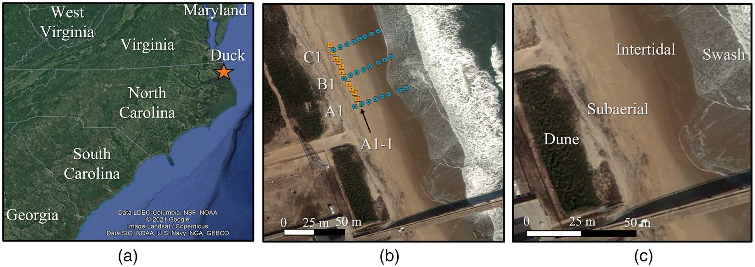
Monthly field measurements were conducted from September 2020 to January 2021, in April 2021, in June/July 2021, and in October 2021 at the USACE Field Research Facility (FRF) in Duck, NC (Fig. 1) along the transect lines shown in Fig. 1(b). During this period, 35 individual surveys were conducted (Table 1) across all four seasons to determine if seasonal trends in bearing capacity, grain size characteristics, and moisture content existed. Sand samples and moisture probe measurements [Figs. 2(a and b), respectively] were conducted during all surveys, generally within a 1- to 1.5-h testing window. Satellite images were taken within the same testing window to avoid bias from changes in the tidal stage. Measurements along each transect stretched from the toe of the dune to the water line; due to fluctuations in water levels impacting the length of the emerged beach profile, the number of stations sampled per survey varied. Generally, stations were spaced 5 m cross-shore, and the three transects were spaced 20 m along-shore. Measurements on December 9, 2020 were spaced 7.5 m cross-shore, and measurements on November 13, 2020 were collected along a single along-shore transect [orange squares in Fig. 1(b)] due to high water conditions. During field measurements, heavy mineral materials were intermittently observed, especially in November–December 2020, and particularly around the second to fourth sampling stations. The presence of heavy minerals was easily identified from sand grain color and resulted in elevated unit weights and moisture content measurements from the moisture probe.
| Date | Time | Sediment sample stations | No. of stations per transect (total collected/no. analyzed) | Total no. PFFP deployments | No. PFFP deployments for analysis | ||
|---|---|---|---|---|---|---|---|
| A | B | C | |||||
| 9/7/2020 | p.m. | A1, A4, A7, B3 | — | — | — | — | — |
| 9/8/2020 | a.m. | A1, A4, A7, B5 | 7/7 | 7/7 | 6/6 | 100 | 100 |
| 9/8/2020 | p.m. | A1, A4, A7, C5 | — | — | — | — | — |
| 9/9/2020 | a.m. | A1, A4, A7, C5 | 7/7 | 7/7 | 6/6 | 100 | 100 |
| 9/10/2020 | p.m. | A1, A4, A7, B4 | — | — | — | — | — |
| 9/10/2020 | p.m. | A4, A7, B4 | — | — | — | — | — |
| 9/11/2020 | a.m. | A1, A4, A7 | 7/7 | 8/8 | 7/7 | 110 | 110 |
| 9/11/2020 | p.m. | A1, A4, A6, A7 | — | — | — | — | — |
| 10/5/2020 | p.m. | A1, A4 | — | — | — | — | — |
| 10/7/2020 | p.m. | A1, A4, A7 | 8/8 | 8/8 | — | 80 | 80 |
| 10/8/2020 | a.m. | A1, A4, A8 | — | — | — | — | — |
| 10/8/2020 | p.m. | A1, A3, A4 | 10/8 | 9/8 | 12/10 | 155 | 130 |
| 10/9/2020 | a.m. | A1, A4, A7 | — | — | — | — | — |
| 10/9/2020 | p.m. | A1, A4, A7 | 9/8 | 9/8 | 11/11 | 87a | 81a |
| 11/9/2020 | a.m. | A1, A4, A6 | 6/6 | 6/6 | 7/7 | 95 | 95 |
| 11/10/2020 | a.m. | A1, A4, A5, C5 | 5/5 | 6/5 | 7/7 | 90 | 85 |
| 11/12/2020 | p.m. | A1, A3 | 3/3 | 4/3 | 4/4 | 55 | 50 |
| 11/13/2020 | a.m. | A1-1, A1-5, A1-12b | 12/12b | — | — | 60 | 60 |
| 12/7/2020 | p.m. | A1, A4, A7, B4 | 8/8 | 6/6 | 6/6 | 100 | 100 |
| 12/9/2020 | p.m. | A1, A4, A6, B3 | — | — | — | — | — |
| 12/10/2020 | p.m. | A1, A4, A7, C2 | 8/8 | 7/7 | 8/7 | 115 | 110 |
| 12/11/2020 | p.m. | A1, A4, A7 | — | — | — | — | — |
| 1/20/2021 | p.m. | A1, A3, A7 | — | — | — | — | — |
| 1/21/2021 | a.m. | B3, B5, B6 | — | — | — | — | — |
| 4/20/2021 | p.m. | A1, A4, A7, B10 | — | — | — | — | — |
| 4/21/2021 | a.m. | A1, A4, A7, C10 | — | — | — | — | — |
| 4/22/2021 | a.m. | A1, A4, A7, B5 | 8/8 | 9/9 | 10/10 | 135 | 135 |
| 4/22/2021 | p.m. | A1, A4, A7, C9 | — | — | — | — | — |
| 4/23/2021 | a.m. | A1, A4, A7, C9 | 10/10 | 10/10 | 10/9 | 150 | 145 |
| 6/29/2021 | p.m. | A1, A4, A7, B9 | 11/11 | 10/10 | — | 105 | 105 |
| 6/30/2021 | a.m. | A1, A4, A7, C10 | 12/12 | 12/12 | 11/12 | 180 | 175 |
| 6/30/2021 | p.m. | A1, A4, A7, B8 | 11/11 | 10/10 | 7/6 | 140 | 135 |
| 7/1/2021 | a.m. | A1, A4, A7, A10 | 11/11 | 11/11 | 12/12 | 170 | 170 |
| 10/13/2021 | Noon | 7c | — | — | — | — | — |
| 10/13/2021 | p.m. | A1, A4, A7, B7, C1, C5, C7, D5c | — | — | — | — | — |
a
Three PFFP deployments conducted per station.
b
Measurements conducted along the cross-shore transect shown in Fig. 1(b) (orange squares).
c
Samples were randomly taken, and no coordinates for the sample location were collected.
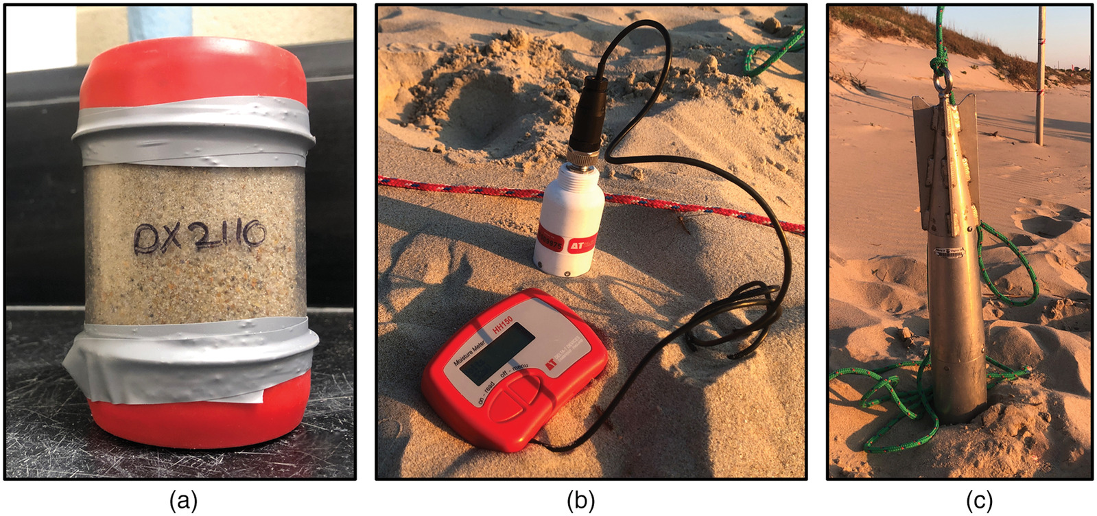
Historically, the beach near the USACE-FRF is composed of a predominately quartz sand that ranges from well-graded to uniform sand, with between 0.3 and 3.84 mm (Birkemeier et al. 1985; Gallagher et al. 2016; Stauble 1992). The site is typically a barred beach and morphological features such as foreshore beach cusps are known to form, typically following storms and during energetic fall, winter, and spring months (Holland 1998). In the present study, sediment sampling was limited by the restricted measurement window of 1–1.5 h. In total, 128 sand samples were carefully collected in 10-cm-long transparent tubes [Fig. 2(a)]; the number and location of samples collected per survey are presented in Table 1. Here, the lowest station number refers to samples near the dune, with the station number increasing while approaching the water line. Moisture contents, unit weights, and grain sizes were determined for each sample. Samples were divided into two 5-cm sections for drying, with the top 5 cm sieved following ASTM D6913-17 (ASTM 2017). At least two physical samples were collected during each survey, with the sampling locations presented in Table 1. Most samples were collected along Transect A, with other samples randomly collected along other transects when visible changes in grain size, mineralogy, or density occurred. At each station, 3–5 volumetric moisture content measurements were collected using a Dynamax SM150 moisture probe [Fig. 2(b)], with readings in mV. These were then converted to moisture content using custom calibration constants developed for the site-specific saltwater and quartz sand (Brilli et al. 2022). Calibration constants were not developed for the heavy mineral sand observed during Fall 2020.
The PFFP blueDrop [Fig. 2(c)] was deployed at 415 stations to measure the quasi-static bearing capacity (qsbc) during 18 surveys in September–December 2020, April 2021, and June/July 2021 (Table 1). Full details of the PFFP data processing can be found in the Supplemental Materials. The dynamic nature of the test indicates that a dimensionless strain rate correction factor needs to be applied; for sandy soils, the logarithmic function is commonly used for submerged sands (Stark et al. 2009, 2012; Stephan et al. 2015; Stoll et al. 2007) and will be applied here. For this study, , a dimensionless coefficient used in strain rate correction, was varied between 1.0–1.5 and compared to computed values of bearing capacity of partially saturated soils. At each station, 3–5 deployments (i.e., individual, independent measurements) were conducted and spaced about 1 m apart, for a total of 2022 deployments as shown in Table 1, with 2004 analyzed. An example of deceleration profiles from the PFFP is shown in Fig. S1 for Station A2 on December 7, 2020. Individual qsbc profiles were calculated for each deployment, with the individual deployments at each station averaged together in 1-cm increments. Then, this average qsbc profile was used to represent each station, for a total of 404 stations. At nine stations, accompanying moisture probe measurements were not collected; these stations were excluded from further analysis. Stations where the penetration depth was were also excluded from further analysis (Albatal et al. 2020). At penetration depths , uncertainty in qsbc increases due to assumptions related to the geometry of the conical tip and the shear failure planes; this resulted in the removal of 153 stations. Finally, stations where heavy minerals were present were also excluded, resulting in 23 stations being removed. These stations were selected based on visual observations in the field, inspection of physical samples, and when moisture probe measurements were significantly higher than the surrounding measurements. This yielded a total of 227 stations from 18 survey periods used for further analysis. In total, about 93.5% of these stations were found within the subaerial or intertidal zones, representing exposed sediments typically imaged by satellites.
Bearing Capacity of Partially Saturated Sands
For partially saturated soils, Vanapalli and Mohamed (2007) suggested that the soil suction () should be included in Eq. (2) in order to account for the effects of partial saturationwhere is the degree of saturation calculated from the porosity and measured moisture content; = friction angle; and = bearing capacity fitting parameter (equal to 1 for sandy soils). For sands, .
(3)
Estimation of Soil Suction
To predict soil suction, the van Genuchten (1980) model is commonly usedwhere = volumetric moisture content; = residual moisture content; = saturated moisture content; is a parameter related to the air entry value; and is a parameter related to the distribution of pore sizes within the sample. From Zambrano-Cruzatty (2021), may be set to 0% in the absence of absorption tests. For sandy soils, is the porosity for volumetric moisture contents and the void ratio for gravimetric moisture contents (Hillel 1998).
(4)
Typically, and are soil-specific parameters measured through laboratory testing (Briaud 2013). Several studies (Chiu et al. 2012; Schaap and Bouten 1996; Scheinost et al. 1997; Vereecken et al. 1989) have proposed pedotransfer functions to quantify the parameters and in order to reduce the need for laboratory tests. Predictors include soil texture (Scheinost et al. 1997; Vereecken et al. 1989), organic content (Schaap and Bouten 1996; Scheinost et al. 1997), bulk density (Schaap and Bouten 1996; Scheinost et al. 1997; Vereecken et al. 1989), and grain size characteristics (Chiu et al. 2012; Schaap and Bouten 1996). Wang et al. (2017) proposed simple relationships for sandy soils that relate and to common grain size distribution parameterwhere = surface water tension dependent on the temperature and salinity of the water (N/m) (Nayar et al. 2014); = particle size that 60% of material passes by weight (mm); and is the coefficient of uniformity (). Eqs. (5) and (6) were developed for sandy soils, grain size distributions without gaps, and drying conditions (Wang et al. 2017). It was assumed that the salinity was based on typical values for Duck.
(5)
(6)
Friction Angles
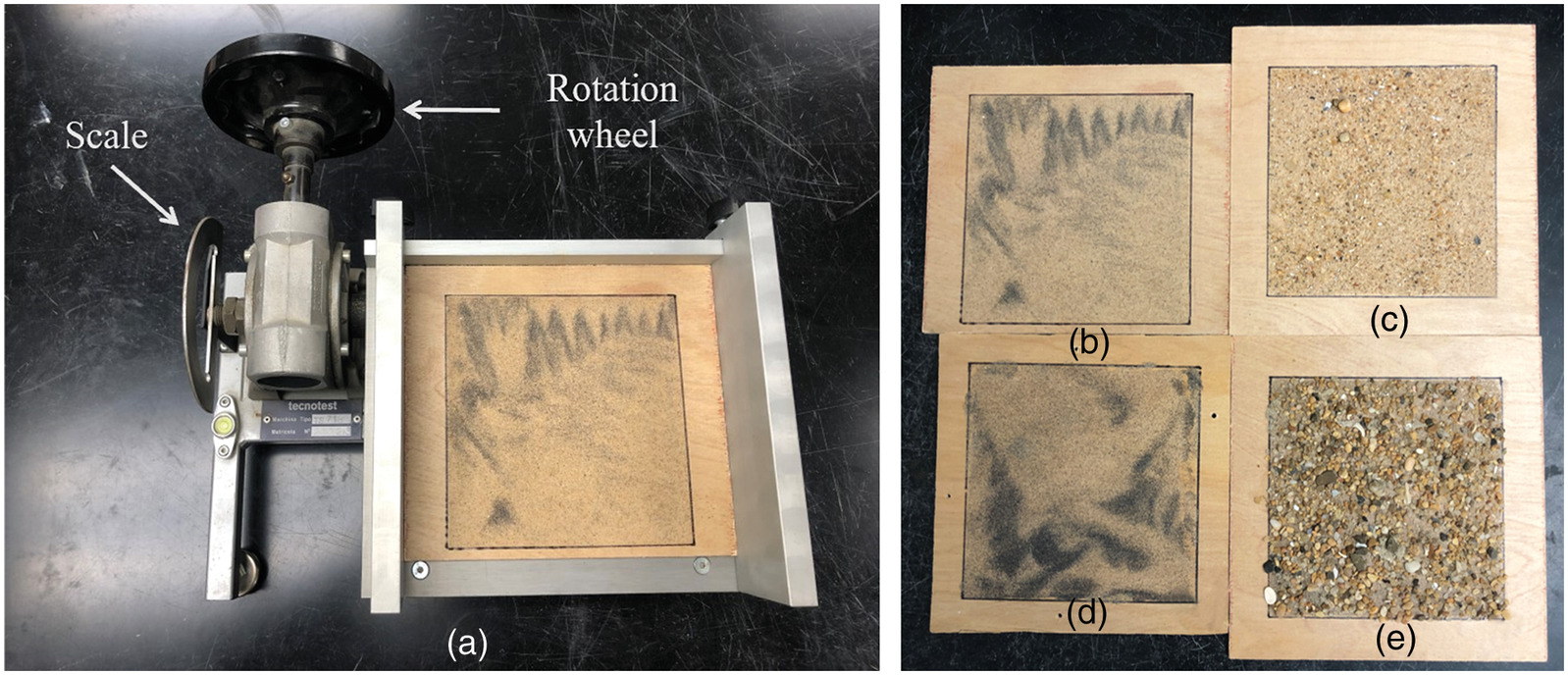
For beach sands at low densities and confining stresses (Dean and Dalrymple 2001), the friction angle may be well-represented by the angle of repose (Briaud 2013; Stark et al. 2017). For this study, a tilt table [Fig. 3(a)] was used to measure the angle of repose for dry sands from Duck. Custom sandpapers were prepared for each sample by gluing a thin layer of sample sand to plywood sheets; the four sheets are shown in Fig. 3(b–e). During testing, about 100 g of sample was pluviated loosely atop the sandpaper. The sample was then tilted manually using the rotation wheel until failure was determined visually as a significant portion of the sample (about 65%–70%) sliding off the sheet. This process was repeated 15 times for each sample to account for variability in determining the failure surface.
Comparison of Field Measurements to Estimated Bearing Capacities
For deployments that occurred simultaneously to sediment sampling (61 total, with 29 used for analysis; seven were excluded due to the presence of heavy minerals and 25 removed due to penetration depths ), relevant information related to the moisture content, penetration depth, grain size characteristics, unit weight, and porosity were used in Eqs. (3)–(6) to calculate bearing capacity. The water temperature was taken from the temperature sensor array (NexSens Inc. Model TS210) located at the end of the pier (USACE 2022); water temperatures ranged from 12.8°C to 25.6°C, resulting in surface water tensions of . For shallow penetration depths, as is common for PFFP deployments, the bearing capacity factors (, ) from Durgunoglu and Mitchell (1973) for cones can be used to estimate the bearing capacity; this approach has been previously applied to PFFP data to estimate the friction angle of subaqueous nearshore sand (Albatal et al. 2020). These bearing capacity factors are dependent upon the friction angle, penetrometer tip angle, relative depth of the penetrometer base (), cone roughness (), and the penetrometer diameter in place of . Here, for the interface between steel and sand (Durgunoglu and Mitchell 1973), and the penetrometer tip angle is 60°. The friction angle used in Eq. (3) was selected based on the of the sampling location.
Sensitivity Analysis
To quantify the effects of the variability in the input parameters of textural characteristics (porosity, , and ) and strength parameters (friction angle, dry unit weight) when estimating the bearing capacity, a sensitivity analysis was performed using the ranges of values observed during field measurements. Here, the estimated bearing capacity [Eq. (3)] was calculated by changing only one variable at a time to determine the effect of each parameter on the estimated bearing capacity, with the remaining variables held at the mean value. The input values of each sediment property ranged from the minimum to the maximum value of each variable. To only investigate the impact of soil characteristics on the estimated bearing capacity, a constant water temperature of 25.5°C was assumed and the footing was assumed to be a square () motivated by the trafficability problem and the approximate shape of a tire-soil contact area; this ratio was selected as it produces the greatest difference in estimated bearing capacities. The bearing capacity and shape factors from Vesić (1973) were used. Additionally, the moisture content was varied, ranging between 0% and 35% to observe how the bearing capacity was impacted by the moisture content. This process was performed for each of the three sand classes individually (fine, medium, and coarse) and for all samples together. The percent difference was calculated as the difference between the maximum and minimum estimated values divided by the maximum estimated value and was reported for each moisture content.
Estimating Moisture Contents from Satellite Images
Gravimetric moisture contents were estimated from the NIR band of the optical image collected on March 14, 2018 of the USACE-FRF in Duck, NC from the WorldView-4 satellite (ground resolution of ) using the framework from Paprocki et al. (2022) and summarized in the supplemental material. For the X-band SAR image collected from the Cosmo-SkyMed 2 satellite on October 8, 2020 at 22:56 UTC and an incidence angle, , of 30.57° (ground resolution of ), volumetric moisture contents were estimated using the model from Paprocki (2022b) for and data that exceeds the very low threshold (). The details of this model can be found in Supplemental Materials. These two images represent case studies randomly selected from a total of 33 SAR and three optical satellite images that were collected during this study.
Bearing Capacity for Trafficability Applications
Hambleton and Drescher (2009) suggested an approximate analytic approach using Eq. (2) to predict the sinkage, (in cm), under steady-state conditions for rigid towed wheels on dry sand. In this model, the load acting on the tire is modeled as an inclined force acting at an inclination angle, where = tire diameter (cm). Hambleton and Drescher (2009) suggested incorporating the inclined load effects into Eq. (2) through either inclination factors or modifications to the bearing capacity factors by assuming the foundation is on a slope. In this study, inclination factors were used. Since the contact area that the tire makes with the sand is assumed to be a rectangle, the bearing capacity factors for rectangles from Vesić (1973), shape factors from De Beer (1970), and inclination factors from Meyerhof (1963) were used and are shown in Supplemental Materials.
(7)
There is not a unified, widely accepted approach to predict the load a vehicle imparts upon the soil, although several models have been developed. Saarilahti (2002a) provides an overview of the wide range of models applicable to forestry-type vehicles and tires, with the models applicable to military vehicles and tires driving on sand summarized in Table 2. Assuming that the contact area of the tire is a rectangle, the tire length is calculated by dividing the calculated area by the tire width . For the bearing capacity formula, the footing width and length are
(8)
| Equation name | Equation | Variables |
|---|---|---|
| Nominal ground pressure | - tire width (m), - tire radius (m) | |
| Komandi (1990) | - road surface constant (4.2-4.4 for loose sand), - tire load (N), - tire width (mm), - tire diameter (mm), - inflation pressure (bar) | |
| Silversides and Sundberg (1989) | - tire load (kN), - tire inflation pressure (kPa) | |
| Kemp (1990) | - tire load (kN), - tire inflation pressure (kPa) | |
| Mean maximum pressure (Priddy and Willoughby 2006) | , where | - tire width (m), - tire diameter (m), - tire deflection upon loading (m), - tire load (kN), - tire inflation pressure (kPa) |
| (Saarilahti 2002b) | ||
| Virtual wheel contact length (Saarilahti 2002a) | , where | - tire width (m), - tire contact length (m), - tire radius (m), - tire sinkage (m), - tire deflection upon loading (m) |
| Schwanghart (1991) | , where | - tire width (m), - tire contact length (m), - tire sinkage (m), - tire deflection upon loading (m) |
The applied stress is calculated using the vertically applied tire load
(9)
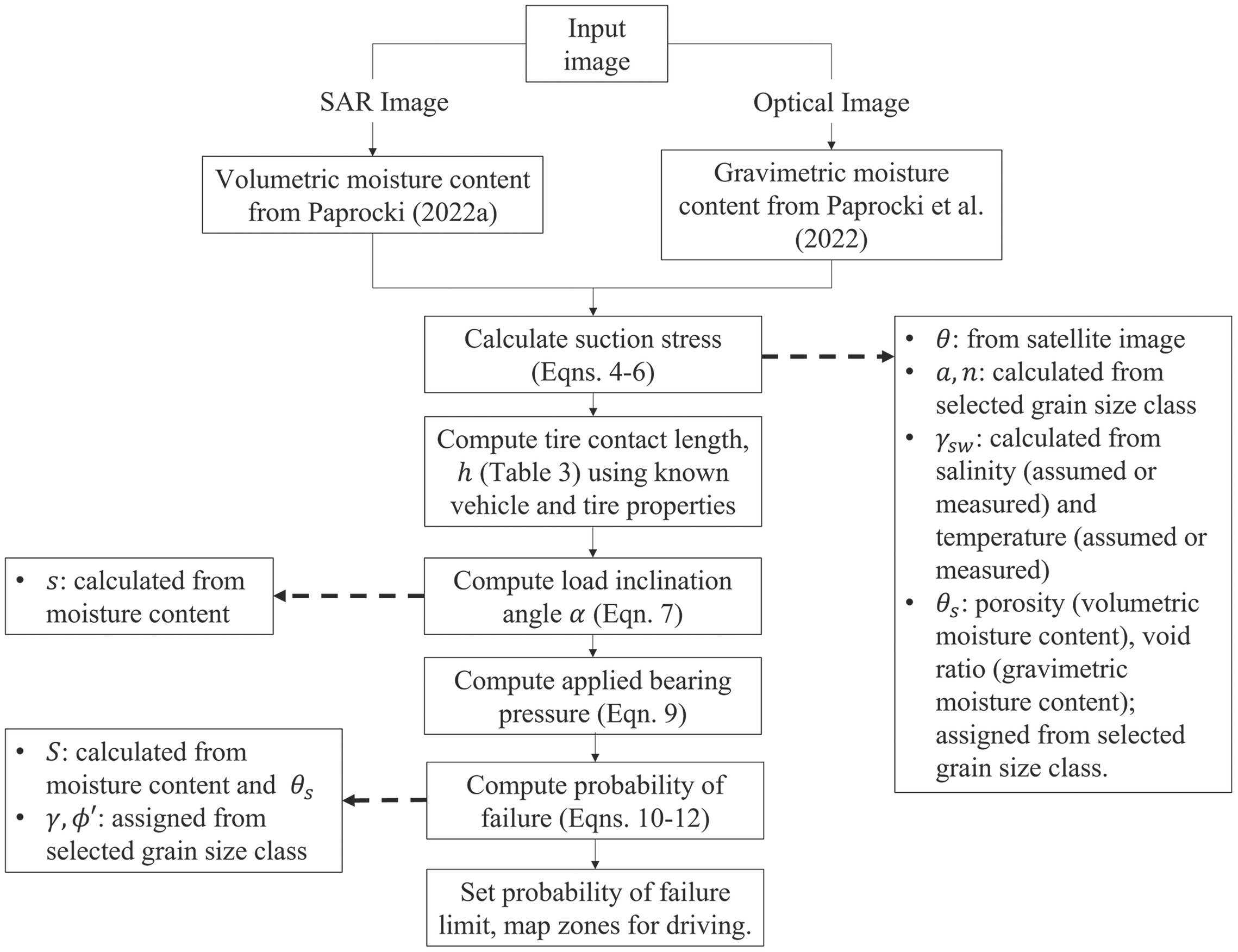
The equation from Table 2 that resulted in a minimum length (and consequently, the maximum ) can then be used to calculate the bearing capacity following the process shown in Fig. 4. For this study, the Lighter, Amphibious, Replenishment, Cargo, 5-Tons (LARC-V), an amphibious military vehicle (Kaczmarek 2004), will be used as the test vehicle. The LARC-V has a net weight with crew and fuel of 8,618.3 kg, a load capacity of 4,535.9 kg (5 tons), and is equipped with four 12-ply super sand flotation tires (diameter of 150.4 cm, a section width of 50.3 cm, and inflation pressures of 68.9–103.4 kPa).
Predicting Soil Suitability for Vehicle Loadings
To determine the suitability of beach sands vehicle loads based on bearing capacity, the estimated bearing capacity is compared to the applied bearing pressure. Since in situ soil properties are known to vary at sand beaches (e.g., Stauble 1992), a probabilistic approach was applied. Most variables used for calculating the bearing capacity can be represented as a matrix of continuous random variables in Eq. (3) and used to define a limit state function,
(10)
When , the soil does not have suitable bearing capacity for trafficability and when , the soil has adequate bearing capacity for trafficability. Thus, the probability that the soil does not have suitable bearing capacity for trafficability (or the probability of failure, ) is defined aswhere is the standard normal cumulative distribution function; = mean of ; and = standard deviation of . Eq. (11) results from a first-order approximation of the limit state function around its mean value (Der Kiureghian 2022). The mean of is found by substituting the mean values for each parameter and the calculated vehicle bearing pressures from Table 2 into Eq. (10). To simplify the calculation of , it is assumed that all variables are uncorrelated; thus, iswhere is the partial derivative of with respect to the th variable in evaluated at the mean; and is the variance of the th variable in . In Eqs. (10)–(12), it is assumed that all input parameters are normally distributed; in the absence of knowledge of the true distribution, this is a common assumption for geotechnical properties (Kadar and Nagy 2017; Lacasse and Nadim 1998).
(11)
(12)
Results
Sand Characteristics
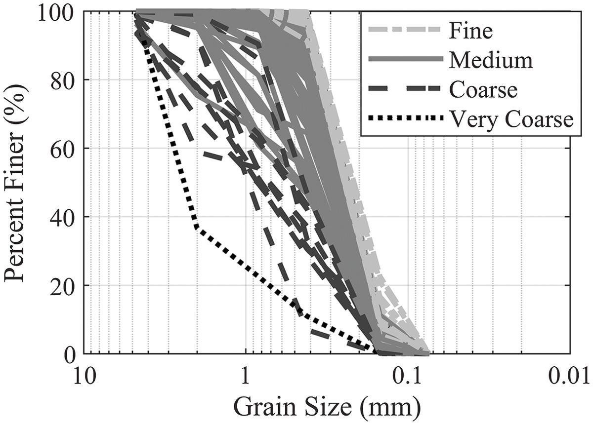
Grain size distribution curves of 127 of the samples collected over all surveys are shown in Fig. 5; see Table S1 for details. Samples were classified according to Wentworth (1922): fine (), medium (), coarse (), and very coarse (). In total, 36 (18.3%) samples classified as fine, 81 samples (63.5%) classified as medium, 9 (7.9%) classified as coarse, and one sample (0.8%) classified as very coarse sand. Following the USCS classification (ASTM 2017), the fine, medium, and coarse sands are poorly graded sands (SP) while the very coarse sample was a well-graded sand (SW). The mean (), standard deviation (), and range of grain size characteristics for each classification are shown in Table 3. Since the very coarse sand class represented only one sample and was collected near the water line at a visible gravel patch at the time of measurements, it will not be discussed further. The cross-shore variation in , , and is shown in Figs. 6(a–c), respectively. The gray x’s represent individual measurements while the orange x’s represent the average values for each station. The variability in the grain size characteristics was found to be generally independent of the season and instead was more strongly related to the location of the beach where the measurements occurred. In general, the grain size characteristics remain approximately constant until Station A7. Samples from A7 onward were generally collected in the swash zone, where considerable variation in grain size has been previously observed (Stauble 1992). Overall, the measurements matched well with observations by Stauble (1992) that were collected monthly at Transect line 62 (modern-day FRF line 1006) are shown in Fig. 6(b) as stars.
| Parameter | Fine | Medium | Coarse | Very coarse | ||||||||
|---|---|---|---|---|---|---|---|---|---|---|---|---|
| Range | Range | Range | Range | |||||||||
| (mm) | 0.25–0.28 | 0.27 | 0.01 | 0.28–0.80 | 0.34 | 0.10 | 0.60–2.05 | 1.10 | 0.43 | — | 2.76 | — |
| (mm) | 0.10–0.16 | 0.15 | 0.02 | 0.15–0.19 | 0.17 | 0.01 | 0.16–0.45 | 0.22 | 0.09 | — | 0.38 | — |
| Porosity | 0.37–0.50 | 0.45 | 0.04 | 0.34–0.53 | 0.44 | 0.04 | 0.33–0.47 | 0.40 | 0.05 | — | 0.43 | — |
| () | 13.3–16.5 | 14.7 | 0.90 | 12.6–17.2 | 14.9 | 1.01 | 14.0–17.8 | 15.8 | 1.39 | — | 14.7 | — |
| (degrees) | 34.0–37.0 | 35.2 | 0.86 | 34.0–36.5 | 35.2 | 0.73 | 36.0–40.0 | 38.1 | 1.07 | 39.0–44.0 | 41.0 | 1.36 |

The dry unit weight, porosity, and friction angles are shown in Table 3 for each sand class. In total, 105 samples were used to find the unit weight and porosity for each class; samples that exhibited heavy mineral materials and those without unit weight measurements were excluded. The porosity ranged between 0.404 and 0.448, which is within the expected range of 0.3–0.6 (Hillel 1998) and with those previously reported for beach sands (Atkins and McBride 1992). As the mean grain size increases, the porosity decreases and the dry unit weight increases as a result of smaller particles filling the pores between larger particles (Hillel 1998); these trends are reflected across the sand classes. The measured angle of repose falls within the expected range of 30°–45°, with 34° as a typical value for dry sand (Glover 1989) and increased with increasing grain size. Previous tilt table tests performed on samples from Duck indicated an angle of repose of 37° (Stark et al. 2017), which may be a result of the slightly coarser material observed and tested (minimum of 0.347 mm). Previous work and correlations (e.g., Decourt 1989; Duncan et al. 2014) indicated that the friction angle should increase with increasing grain size. The fine and medium sands exhibited the same values for the angle of repose, likely due to the similarities in the grain size distributions of the two classes (Fig. 5).
Sensitivity Analysis
The results of the sensitivity analysis are shown in Fig. 7 as a function of the moisture content for the three sand classes and all sand data combined; the presented values represent the maximum percent differences. Overall, the friction angle (dashed line) had the most significant impact on the estimated bearing capacity, with percent differences of 32%–48.4% for the different sand classes and 81.0%–81.7% for all three sand classes together. This is a result of the friction angle appearing in multiple locations in Eq. (3); particularly, the bearing capacity factors [ and ; see Eqs. (S9 ) and (S10 ) for details] vary significantly as a result of the varying friction angle. For the total range of friction angles, varies between 38.4 and 220.8 and varies from 42.2 to 118.4, which would result in a wide range of bearing capacities. For the friction angle, the percent difference did not exhibit a strong relationship with the moisture content, with the percent difference varying by for all four cases. Only dry angles of response were used to represent the friction angle since this represents the minimum value. The angle of repose was not tested at a varying moisture content despite the known influence of moisture content (Stark et al. 2017).
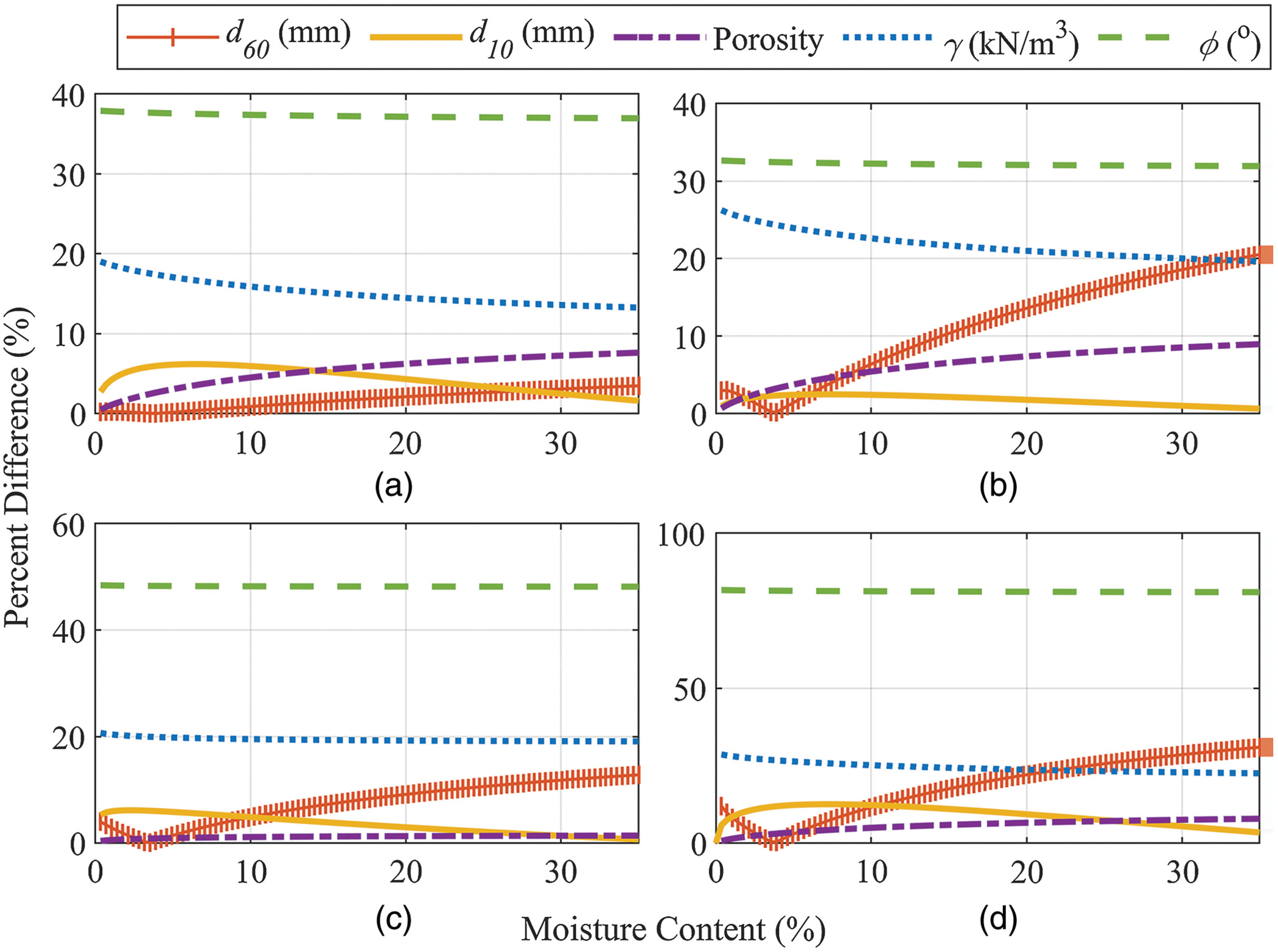
The impact of the remaining four properties (, , porosity, and dry unit weight) on the estimated bearing capacity related noticeably to changes in the moisture content. Particularly, the had a pronounced relationship with the moisture content. The two parameters that are related to the , [Eq. (5)] and [Eq. (6)], decrease with increasing ; and are then used to compute the suction stress [Eq. (4)]. The parameters and are not dependent upon the moisture content and only vary as a function of the . The suction stress, however, is strongly related to the moisture content, thus impacting the bearing capacity. For small values of moisture content, the calculated suction stress (and, in turn, bearing capacity) increases for increasing values of . At a moisture content of about 3.9%, however, higher suction stresses and bearing capacities occur for smaller values of ; this trend continues as the moisture content increases beyond 3.9%. Independent of , suction stress decreases and the bearing capacity increases as the moisture content increases. Across all four sand cases, the percent difference associated with a varying (solid line with bars in Fig. 7) on the bearing capacity decreased while increasing the moisture contents to about 3.9%; at this moisture content, the smallest percent difference was observed (0.1%–0.4%). Then, the percent difference increased as the moisture content increased. When increasing moisture contents beyond about 3.9%, the calculated suction stress decreases with an increase in . At a moisture content of 35%, the largest percent difference occurred for all sand classes combined (31.0%), followed by the medium (20.5%), coarse (12.8%), and fine (3.5%) and classes.
The impact of (solid line in Fig. 7), which is used to compute the parameter [Eq. (6)], also exhibited a pronounced relationship with moisture content, though to a lesser extent than the . The parameter , and in turn, the suction, decreases with an increasing ; this trend was consistent across the entire range of moisture contents. The largest percent difference (12.6%) was observed when considering data from all sand samples at a moisture content of 7.4%. For the fine and coarse sand classes, the maximum percent difference was 6.2% at moisture contents of 6.4% and 2.1%, respectively, while for the medium sand class the maximum percent difference was 2.5% at a moisture content of 7.1%. Overall, the had a lower impact on the bearing capacity than the . The porosity was used as the saturated water content, , in Eq. (4) (Fig. 4) to calculate the suction as well as the degree of saturation in Eq. (3). Across all four cases, variation in the porosity (dot-dash line in Fig. 7) led to increasing percent differences with increasing moisture content. For all four sand cases, the maximum percent difference when varying the porosity was less than 10%, indicating minimal impact. Finally, the bearing capacities estimated using a varying dry unit weight (dotted line in Fig. 7) exhibited percent differences that decreased with increasing moisture content. When varying the unit weight, the percent difference ranged from 13.3% to 19.0% for fine sand, 19.7% to 26.2% for medium sand, 19.1% to 20.7% for coarse sand, and 22.6% to 28.6% when considering data from all sand samples.
Field Measurements of Bearing Capacity
An example of the typical cross-shore trends in moisture content, peak qsbc at , and penetration depth are shown in Fig. 8 for the survey on October 8, 2020 [Transects A, B, and C; see Fig. 1(b)]. Little variability in moisture content and bearing capacity was observed across seasons; instead, it was found that trends in bearing capacity and moisture content were strongly related to the cross-shore beach zone where measurements occurred and storm events. The moisture content [Fig. 8(a)] increased cross-shore toward the water line. The standard deviation between individual measurements at each station ranged from 0.05% to 16.6%, with an average of 1.7%, when excluding stations where heavy minerals were observed. Higher standard deviations were observed during storm events (1.8% to 16.6%, average of 6.9%) versus non-storm conditions (0.05% to 9.4%, average of 1.5%). High standard deviations were occasionally observed in the subaerial zone, especially from September to December 2020 when heavy mineral material was abundant and may have been included in the sand at the site at depth but was not observed on the surface or in the samples. The highest standard deviations in moisture content (average standard deviation of 4.2%) occurred at mean moisture contents of 10%–22.5%; these moisture contents generally occurred across the entire intertidal zone.

The qsbc [Fig. 8(c)] generally increased and penetration depths [Fig. 8(b)] decreased while approaching the water line, following trends observed previously (Brilli and Stark 2020; Reeve et al. 2018; Stark et al. 2022). Over all surveys, the impact velocity ranged between 2.31 and and penetration depths ranged between 1.3 and 24.6 cm for individual deployments of the PFFP. Most surveys exhibited a range of penetration depths cross-shore, with deeper depths observed in the subaerial zone and shallower penetrations in the swash; examples of these trends from a single survey are shown in Fig. 8(b). Impact velocities varied somewhat between surveys, representing the larger user dependence of the device in air than in water. However, analysis resulted in similar magnitudes of qsbc between surveys despite differences in the impact velocities, and little variability in the impact velocity was observed (standard deviations of about in most cases; 0.3%–27.8% of the mean, with an average of 3.6%) between deployments at a given station. Deployments in the swash exhibited the most variability in terms of PFFP measurements, likely a result of the rapidly changing conditions in this zone (e.g., grain size, unit weight, and swash uprush/backwash) occurring in this region (Dean and Dalrymple 2001; Stark et al. 2022).
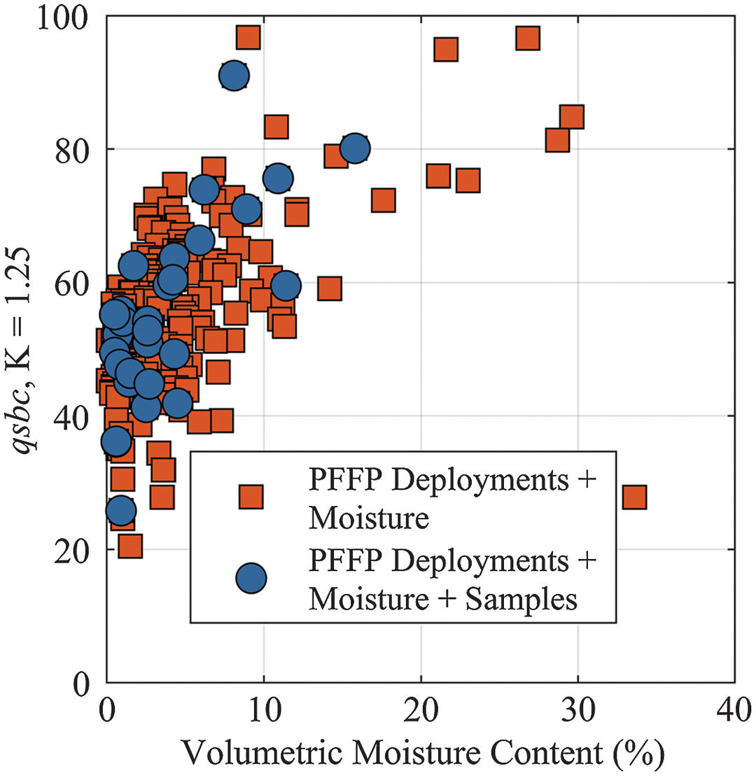
Fig. 9 presents the moisture content measured using the moisture probe and the corresponding qsbc using for stations where sediment samples, moisture probe, and PFFP measurements were collected simultaneously (blue circles) and stations where only the moisture probe and PFFP were used simultaneously (orange squares). For stations where deployments of the PFFP and sediment sampling occurred simultaneously (29 of 61 stations of those included in analysis; moisture contents of 0.5%–15.8%), the values of qsbc computed using were compared to the estimated bearing capacity computed from the measured sand sample characteristics and the bearing capacity factors for cones from Durgunoglu and Mitchell (1973). The qsbc that resulted in the closest match was selected as the measured qsbc. The comparison between the measured and estimated bearing capacities are shown in Fig. 10(a), with a correlation coefficient, , of 0.83.
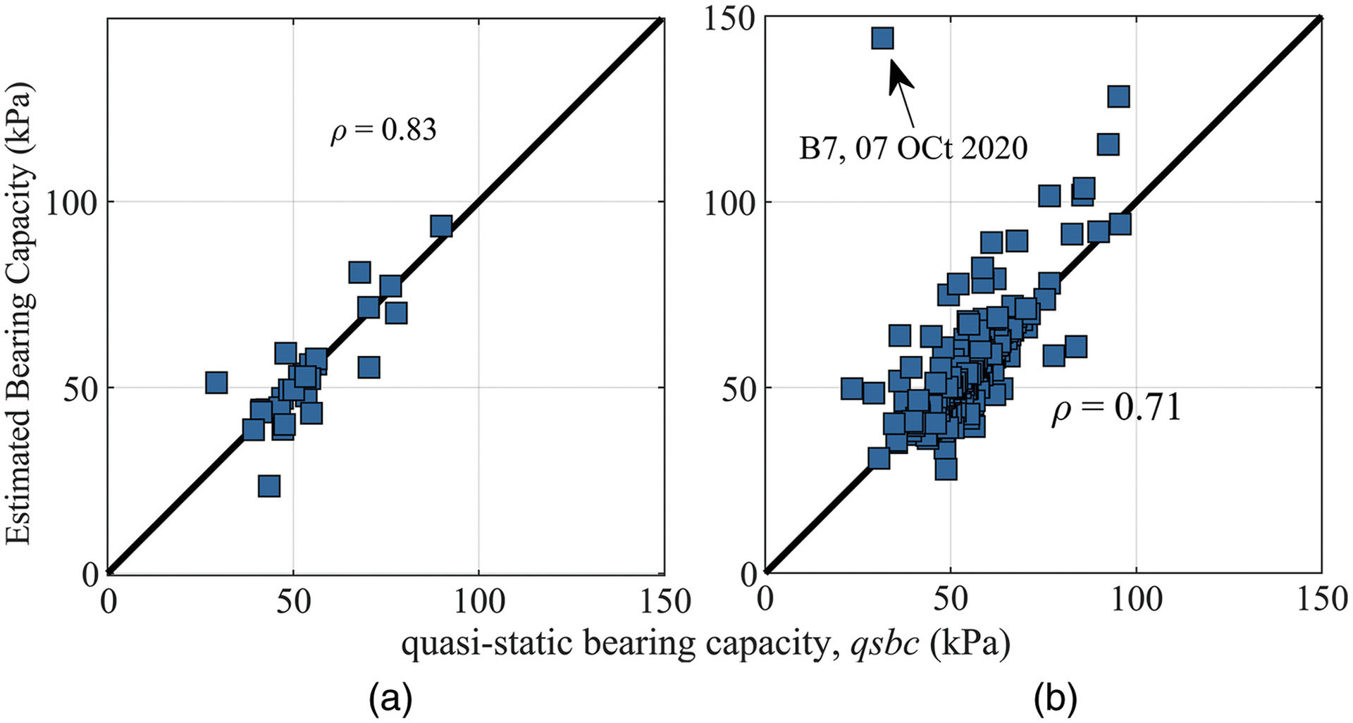
Due to the excellent match between the measured qsbc and the bearing capacity predicted using measured sand characteristics, the bearing capacity was then calculated using assumed sand characteristics (227 of 404 total stations) and the measured moisture content at that station. For these stations, volumetric moisture contents ranged from 0.1% to 33.6%, the location of maximum qsbc ranged between 7 and 17 cm, and peak qsbc varied between 23.4 and 95.7 kPa. The medium sand characteristics measured in situ (Table 3) were used as the assumed sand characteristics to compute the bearing capacity for all stations. Medium sand represented 63.5% of all samples collected, and, when combined with fine sand (which exhibits similar characteristics to medium sand; Table 3) represented 81.7% of samples collected. From this, the measured qsbc and the bearing capacities estimated using the medium sand characteristics are shown in Fig. 10(b), with .
To examine the model fit for estimating the bearing capacity using the medium sand class characteristics, the residuals of the estimated bearing capacities were computed, and are shown in Fig. 11. The residuals typically ranged between and 33.1 kPa (negatives represent underestimates) with an average residual of 1.32 kPa, with 194 stations (or 85.5% of stations) exhibiting estimates within . At one station, B7 on October 7, 2020, the bearing capacity was overestimated by 112.4 kPa (i.e., the bearing capacity model suggested stronger sands than measured by the PFFP) and exhibited the highest moisture content measured (33.6%). Previous studies found that PFFP measurements within the swash/water generally exhibit higher strengths and penetration depths (Brilli and Stark 2020; Reeve et al. 2018; Stark et al. 2022), typically a result of in situ densification from wave action (Heathershaw et al. 1981). However, station B7 exhibited a deeper penetration depth (15 cm) and lower measured strengths () than typically observed within the swash. This reduction in strength may be a result of environmental factors such as the development of hydraulic gradients and swash dynamics, which have been observed to occur in sand beds under non-storm conditions (Horn et al. 1999; Stark et al. 2022). For sand with , Horn et al. (1999) found that large upward (negative) hydraulic gradients can occur in the uppermost layers (about 1–2 cm depth) of the bed under swash retreat, potentially leading to bed fluidization (Packwood and Peregrine 1980), reduced strengths, and increased PFFP penetration depths. This process was not considered in the model for estimating CI [Eq. (1)] nor in Fig. 4. To determine whether the development of hydraulic gradients could reduce the measured bearing capacity, a simple analysis was performed. For foundations subjected to seepage forces from groundwater flow, Veiskarami and Kumar (2012) suggested replacing the unit weight in Eq. (3) with , where is the submerged unit weight and is the hydraulic gradient. Upward-directed flows decrease the bearing capacity (), while downward flows () increase in the bearing capacity. Horn et al. (1999) found maximum upward gradients of 2.3 to 2.7 in the upper 1–2 cm of the sand bed, which are sufficient to fluidize the bed (Packwood and Peregrine 1980). These hydraulic gradients were tested in Eq. (3) by replacing with . This resulted in an estimated bearing capacity of 37.8 kPa, with a residual of (slightly underestimated bearing capacity).

Bearing Capacity for Trafficability Applications
For the optical image, the estimated moisture contents are shown in Fig. 12(a) to the north of where field measurements occurred [Fig. 1(b)]. Lower moisture contents were observed near the toe of the dune and increased toward the water line, following previously observed trends (Paprocki et al. 2022). The estimated moisture contents for the SAR image are shown in Fig. 13(a) in the general vicinity of field measurements [Fig. 1(b)]. The SAR image confirmed the same trends in moisture content as the optic image. However, higher values of moisture content were observed near the toe of the dune due to the lower limit set by the SAR model (lower limit of ). The CI [Eq. (1)] was estimated using the estimated moisture contents from both the optical [Fig. 12(b)] and SAR [Fig. 13(b)] images. For the optical image, lower CI values were observed near the toe of the dune than for the SAR image, in line with the differences in the estimated moisture contents. In both images, higher CI values are observed near the water line where higher moisture contents are expected, consistent with the expected trends (Sullivan and Anderson 2000).

Case Study: Estimating Bearing Capacity for LARC-V Trafficability
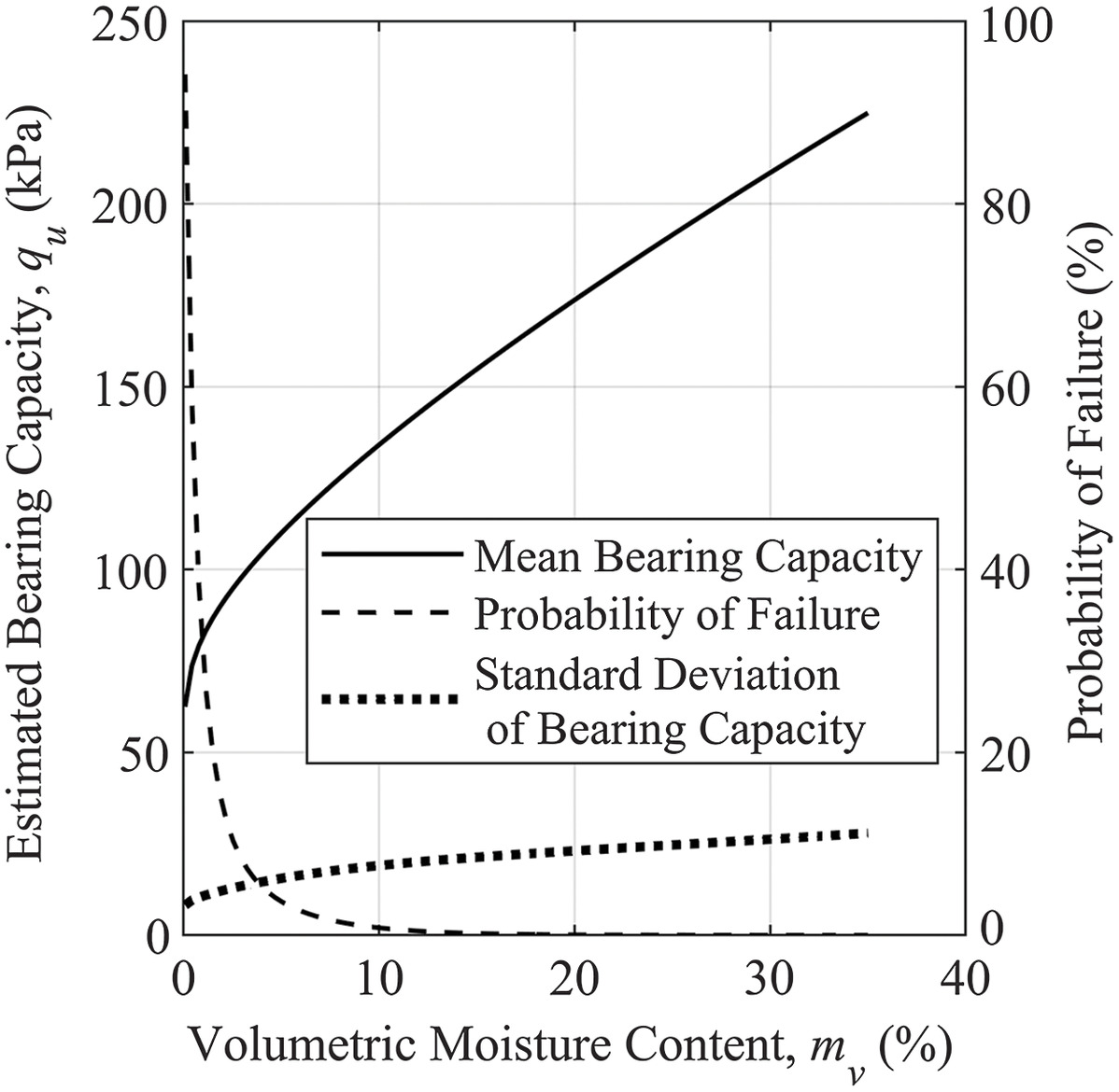
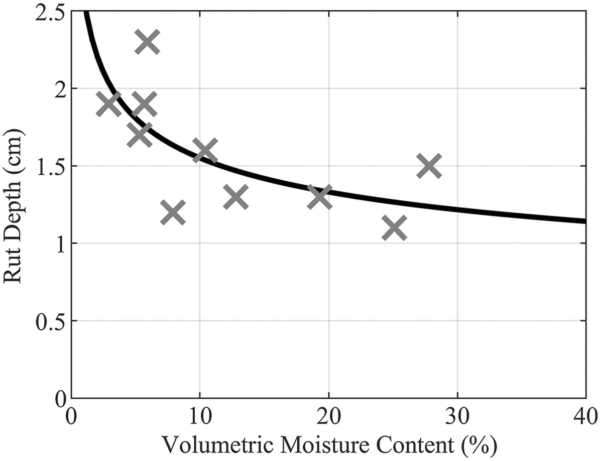
The estimated mean (solid black line) and standard deviation (dotted line) of the bearing capacity for the LARC-V is shown in Fig. 14 as a function of the moisture content, following the procedure shown in Fig. 4. Here, the parameters for medium sand from Table 3 were selected for calculating the bearing capacity since this class represented the majority (63.5%) of samples collected, and when combined with the fine samples (which exhibit similar characteristics to the medium samples, see Table 3), represented 81.7% of samples collected. It was assumed that the LARC-V was loaded to the gross weight of 8,618.3 kg and tires were inflated to a pressure of 68.9 kPa. Sinkage was calculated using the relationship shown in Fig. 15, which is based on field measurements of rut depth and moisture content during the October 2021 measurements. It should be noted that rut depth (and not sinkage) was measured, but it is assumed that they are equal since the difference between them is small (Affleck 2005). The applied bearing pressure was calculated as a function of the sinkage, and in turn, moisture content, ranging from 74.7–76.3 kPa, with lower values associated with lower moisture contents. The standard deviation of the moisture content was calculated using the equation derived from field measurements of the moisture probe [Eq. (S7 )]. From Fig. 14, the estimated mean and standard deviation of the bearing capacity both increased as the moisture content increased.
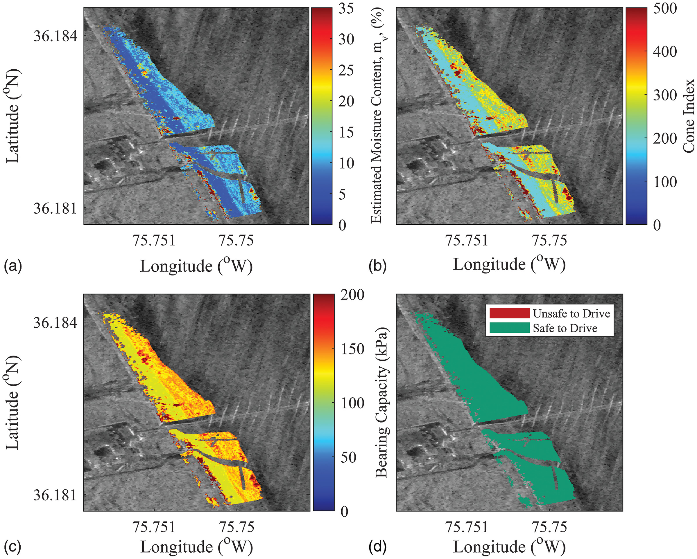
Using the process shown in Fig. 4, the bearing capacity estimated from the moisture contents based on the optical image is shown in Fig. 12(c) and those based on moisture contents from the SAR image are shown in Fig. 13(c). For the optical image, where the gravimetric moisture contents were estimated, the void ratio was used for calculating the suction stress [Eq. (4)]. For the SAR image, porosity was used to calculate the suction stress since volumetric moisture contents were estimated. The most suitable paths for driving on the beach (based on the probability of inadequate bearing capacity) are presented in Fig. 12(d) for the optical image, and in Fig. 13(d) for the SAR image assuming a probability of failure of 10%. For the optical image [Fig. 12(d)], areas near the toe of the dune are unsuitable for trafficability, which corresponds to areas of lower bearing capacity [see Fig. 8(c)]. However, the SAR image [Fig. 13(d)] indicates that the entire area of the beach is suitable for driving, likely a result of the lower limit of the moisture content used when modeling the moisture content.
Discussion
Sand Characteristics and Estimated Bearing Capacity
From sensitivity analysis (Fig. 7), the selected friction angle has the greatest impact on the bearing capacity since the friction angle explicitly appears in Eq. (3) and in the equations for the bearing capacity factors [see Eqs. (S9 ) and (S10 )]. Therefore, care should be given toward selecting the sand class (since this dictates the friction angle) in order to not overestimate the strength. Overprediction of the friction angle would lead to potentially unsafe driving conditions and increase the risk of bearing capacity failure. Thus, if the literature suggests that both medium and coarse sand are present at the site, it would be conservative to select the medium sand characteristics. For example, Stauble (1992) [black stars in Fig. 6(b)] suggested that medium sand dominates the subaerial zone for non-storm conditions [a distance from the dune of 8 and 17 m in Fig. 6(b)], with slightly coarser material observed during storm events. This coarse material likely resulted from finer material being washed away during high water conditions during storm events and wind transport during fair conditions (Stauble 1992). Thus, the use of a lower friction angle in the subaerial would yield conservative estimates for bearing capacity. During non-storm conditions, the intertidal (black stars at about 30.6 m from the dune) exhibited significant variation in grain sizes, ranging from fine () to very coarse () sands. However, medium sand still dominates [about 45.5% of all samples observed in Stauble (1992)], indicating that it is still reasonable to use the medium sand characteristics to predict the strength in the intertidal zone. From Glover (1989), the angle of repose for loose sands should range between 30° and 45°, with 34° a typical value for dry sands. Therefore, in the absence of grain size information, friction angles of 30°–34° can be used to provide a conservative estimate of the bearing capacity.
When using the bearing capacities derived from assumed sand characteristics using data from in situ measurements [characteristics for the medium sand class from Table 3; Fig. 10(b)], there is general agreement between the measured qsbc and estimated bearing capacities, suggesting that the presented approach (flow chart in Fig. 4) can be applied for average (i.e., non-storm) beach conditions. While 194 stations had residuals smaller than 10 kPa (Fig. 11), the remaining 33 exhibited residuals outside this range. Of these, 11 exhibited negative residuals, indicating that the bearing capacity was underestimated, representing conservative results. The remaining 22 exhibited overestimates of the bearing capacity to some degree. In total, 14 of these stations were located within the subaerial zone during normal (non-storm) conditions. The subaerial zone is known to exhibit low relative densities and unit weights, with unit weights likely lower than the average values used here (Table 3). NAVFAC (1986) suggests that loose, uniform, fine-to-medium sands, which would typically characterize the subaerial zone, can have unit weights as low as . In this study, 38% of medium sand samples collected at Station A1 exhibited moist unit weights less than this when using the average dry unit weight to estimate the moist unit weight. This indicates that it may be conservative to use slightly lower mean values of dry unit weight in this region in order to not overestimate the strength, especially given the influence of the unit weight on the bearing capacity (Fig. 7). Additionally, four measurements with residuals occurred in December 2020 when a significant amount of heavy mineral material was observed near the toe of the dune. Two of those measurements exhibited moisture contents (8.0%–11.3%) above the expected range (Paprocki et al. 2022), pointing at the presence of heavy mineral material within the soil that was not visible, resulting in elevated moisture contents and overestimated bearing capacities. Finally, organic materials were observed at Station B4 on September 9, 2020, likely elevating the measured moisture content.
High residuals were also observed at stations where moisture contents vary significantly. One such station was located at the transition between the subaerial and intertidal zones (where the moisture content can vary rapidly over short distances), while the other two were measured near the edge of the water in the lower intertidal zone (where the moisture content at the edge of the water can vary rapidly in response to wave runup and tides). Additionally, four of those measurements were collected during storm conditions on November 12, 2020 [about 7.5–8.5 cm of rainfall over 48 h (NOAA 2021b)]. For these six stations (four during storm, two near the edge of the water), wetting occurred during measurements, and the framework for estimating the bearing capacity may not be applicable to these measurements; Eqs. (5) and (6) were developed for drying (and not wetting) conditions to estimate the suction stress. During in situ measurements, PFFP deployments and moisture probe measurements were taken within minutes of one another, but even during this short time period large variations in moisture contents were observed. This highlights the dependence of the bearing capacity on moisture content as demonstrated by the sensitivity analysis (Fig. 7), suggesting that accurate moisture contents and consideration of variability are needed to safely estimate the bearing capacity.
Another factor likely influencing the measured bearing capacities within the intertidal and swash zones is the variation of grain sizes. Particularly, the had a significant impact on the estimated bearing capacity in the sensitivity analysis through its relationship to the moisture content (Fig. 7). At higher moisture contents (), the bearing capacity was almost always overestimated (Fig. 11), corresponding to when a larger percent difference was observed in the medium sand class [Fig. 7(b)]. Throughout the survey sequence, surficial gravel (coarser sediments) as well as a wider range of grain sizes (Fig. 6) were found near the water line (within the intertidal and swash zones). This trend has been observed in previous studies of sandy beaches (Abuodha 2003; Dingler and Reiss 2002; Gallagher et al. 2016, 2011; MacMahan et al. 2005; Prodger et al. 2016, 2017; Reniers et al. 2013; Stark et al. 2022; Stauble 1992; Thornton et al. 2007). Even for beaches that are usually composed of fine and medium sands, larger grains have been observed during and following storm events (Dingler and Reiss 2002; Gallagher et al. 2011; Prodger et al. 2016, 2017; Stauble 1992), indicating that the characteristics of coarse sands from Table 3 may be applicable at the water line or during storm events. Future work will focus on spatially mapping the distribution of grain sizes within the swash zone to improve bearing capacity estimates in this region.
The remaining station that exhibited a residual was B7 on October 7, 2020, which was located in the swash at the time of measurements. While larger grain sizes than those found for the medium sand class likely occurred in this region (Fig. 6), when a of 3.81 mm [the largest observed by Stauble (1992) in the intertidal zone] was tested, the bearing capacity was still overestimated. This indicates that, despite the importance of the grain size on the estimated bearing capacity, other external forces, such as upward-directed hydraulic gradients and swash processes, are likely key processes influencing the qsbc near the waterline. The impact of these pressure gradients can be captured with a simple calculation using values presented in the literature to represent a theoretical “worst case” scenario for bearing capacity within the swash. Of note, the large negative gradients measured by Horn et al. (1999) used in this study (2.3–2.7) occurred during flood (rising) tide conditions, with positive (downward) gradients dominating during ebb (falling) tides, indicating that the tidal stage also has an impact on the development of pressure gradients that may reduce the bearing capacity. Measurements in October 2020 began at low tide with Transect A, with the final transects, B and C where the low strengths were observed, occurring during the start of flood tide (NOAA 2021a). Thus, it may be suggested to use upward-directed hydraulic gradients when estimating the bearing capacity as a conservative boundary during flood tide. In the future, measurements of the bearing capacity and pressure gradients should be collected simultaneously to better understand their relationship.
Bearing Capacity for Trafficability Applications
Uncertainty in estimating the bearing capacity may arise due to three sources: inherent variability of the soil properties due to natural processes altering the soil, measurement error, and transformation uncertainty (Phoon and Kulhawy 1999). To account for the inherent variability of soil properties, a probability of inadequate bearing capacity [Eqs. (10)–(12)] was computed, assuming a normal distribution. Baecher and Christian (2005) found this to be a reasonable assumption, likely resulting in an overestimation of the probability of failure. In Eqs. (10)–(12), it was assumed that the input parameters followed normal distributions. This is a common assumption for geotechnical properties, as most geologic processes follow either a normal or lognormal distribution (Kadar and Nagy 2017; Lacasse and Nadim 1998). Lacasse and Nadim (1998) reported that the friction angle is normally distributed, with coefficients of variation (COV, ) of 2%–5%. Lacasse and Nadim (1998) also reported that, for all soils considered together, the submerged unit weights and porosities were also normally distributed, with COVs of 0%–10% and 7%–30%, respectively. Duncan (2000) found COVs of 3%–7% for the unit weight and 2%–13% for the effective stress friction angle when analyzing the data reported from a number of sources. Finally, From Table 3, the COVs range from 8.9% to 12.5%, 6.1% to 8.8%, and 2.1% to 2.8% for the porosity, unit weight, and friction angle, respectively, and are within the expected ranges from Lacasse and Nadim (1998) and Duncan (2000). Phoon et al. (1995) suggested COVs of 5%–11% for the effective stress friction angles of sands, and are higher than those presented in Table 3; however, the test method was not specified for these data, and thus, a direct comparison cannot be made. Limited data is available regarding the distribution of grain sizes, though Kadar and Nagy (2017) assumed normal distributions for and calculated a COV of 26% for the of a sand/silty sand; this value similar to the values observed for medium (29.4%) and coarse (39.1%) sands. However, further testing is required to investigate the distributions of the grain sizes at sandy beaches. Lacasse and Nadim (1998) found that varying the distribution function of soil parameters had a minimal impact on the computing the probability of failure, indicating that the selection of normal distributions for sediment characteristics is an acceptable assumption.
For both images, moisture contents were averaged over a area, or an area of for the SAR image and an area of for the optical image. During field measurements, each station had five measurements collected that were spaced about 1 m apart. Most stations (for non-storm measurements and when stations with heavy minerals were excluded, 523 of 609 stations) exhibited limit variability (standard deviations ) between the five measurements of moisture content, indicating that the resolutions of the images used are likely suitable to estimate the moisture content and in turn, sediment strengths. Additional scrutiny should be given to estimates at the edges of beach zones and in the presence of geomorphological features, where more variation was observed between the individual measurements at each station.
The estimated CI values [Figs. 12(b) and 13(b) for the optical and SAR images, respectively] indicate that the entire area of the beach would be suitable for trafficability, as a minimum CI of 60 is required for the LARC-V to safely traverse sandy beaches (Jenkins 1985). However, this approach does not account for variable soil properties (i.e., changes in grain sizes, unit weights, friction angles, and porosities) beyond the moisture content. The estimated probability of failure [Figs. 12(d) and 13(d)], which does incorporate this variability, can be used to select the best path for driving across the beach and contribute to risk reduction. For both the high-resolution optical and SAR data, both the estimated moisture contents and bearing capacities followed the expected trends from field measurements (Fig. 8), with lower strengths observed near the toe of the dune and higher strengths near the water line. The estimated moisture contents from the optical image [Fig. 12(a)] spanned the entire range of possible moisture contents, with lows of about 0% and peaks of 25%. Near the toe of the dune, there were high estimates of moisture content (about 10–15%), which may be a result of both increased surface roughness (Dean and Dalrymple 2001) and organic material, both which are known to decrease the reflectance and impact the estimated moisture contents (Baumgardner et al. 1986; Johannsen 1969). This results in potentially erroneous estimates of bearing capacity, and in turn, maps of safe driving. Thus, it may be reasonable to use a lower mean moisture content (i.e., about 2–3 standard deviations below the mean) for this region in order to more accurately assess the best path for driving in this region.
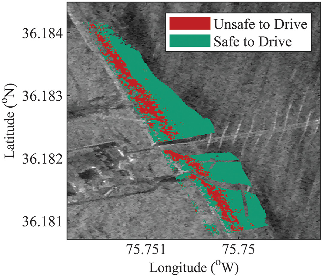
For the SAR image, both the estimated moisture contents [Fig. 13(a)] and bearing capacities [Fig. 13(c)] near the toe of the dune were higher than those estimated from an optical image. For the model used here (Paprocki 2022b), there is a lower limit for the estimated moisture contents that is a function of the incidence angle of the image ( ; (Oh 2004)). This lower limit is 6.8% (based on ) for the image used in this study, which would result in a bearing capacity of 119.2 kPa and a probability of failure of 2.1% (Fig. 14). The minimum moisture content measurement from October 8, 2020 [Fig. 8(a)] was 0.8%, which results in a bearing capacity of 76.7 kPa and a probability of failure of 46.8% (Fig. 14). From the October 8, 2020 measurements, about 48% of all measured moisture contents fall below the lower limit of 6.8%. These moisture contents occurred in the subaerial zone, which is generally characterized by lower strengths and unit weights. Therefore, in order to not overestimate the strengths in this zone, an alternative approach for predicting the most suitable path for driving on the beach is shown in Fig. 16 for the SAR image. Here, regions where the estimated moisture content is are classified as “unsafe for driving” and regions where the estimated moisture contents were are classified as “safe to drive.” While this map is not an explicit representation of strength, it is guided by a need to not overpredict the suitability of soils for trafficability and instead address the most suitable path for driving based on estimated moisture contents.
The two images selected for estimating the moisture content and strengths are representative cases of the range of images tested. For the optical image from March 14, 2018, the estimated moisture contents fell well within the expected range. Similar trends were observed for all other images tested, including different grain sizes, resolutions, and sites (Paprocki et al. 2022), indicating that the approach proposed in Fig. 4 can be used to estimate the bearing capacity for other high-resolution optical images with NIR bands. During measurements in 2020–2021, 28 X-band SAR images were collected, with a further five collected in 2018–2019, including three collected at approximately the same time as the optical images. For the model presented (developed for , see the supplemental materials for details), similar trends of moisture contents as seen in Fig. 13(a) have been observed across a range of seasons, indicating that the presented approach can likely be applied for a range of seasons.
As a next step, the use of other satellite sensors to estimate the moisture content should be tested. In this study, only high-resolution X-band and multispectral images were used. C-band (wavelengths of 3.5–7.5 cm) data from satellites such as Radarsat-2 (ground resolutions of about ) are an alternative candidate for estimating the moisture content, especially due to the similar ground resolutions to optical images tested in Paprocki et al. (2022). Lower resolution satellites such as the C-band Sentinel-1 SAR and the optical Sentinel-2 sensors (resolutions of about ) likely do not have the appropriate resolutions to detect the subtle changes in moisture content that occur at sandy beaches of similar widths (on the order of tens of meters depending on tidal stage), especially given the dependence of the bearing capacity on accurate measurements of the moisture content (Figs. 7 and 11). However, they may be able to provide information regarding changes in ground conditions at beaches, such as grain sizes, beach slopes, and water lines. Sentinel-1 and -2 are publicly available and have revisit times of 5 days, meaning that data related to ground changes can be collected regularly to inform the detailed moisture content analysis from the high-resolution X-band SAR and WorldView optical data. Particularly, Sentinel-2 data has been used to map shoreline positions (Vos et al. 2019a, b) and beach slopes (Vos et al. 2020), which are important factors toward identifying the location of bare soils and estimating the moisture contents and, in turn, strength.
Conclusion
The bearing capacity of sandy beach soils was estimated following a novel framework that used remotely sensed moisture contents and standard sand characteristics. Toward this goal, the seasonal and spatial variability of sediment characteristics (, , dry unit weights, porosities, moisture contents, and angles of repose) were documented over a one-year period for a quartz sand beach; these properties were assumed to followed normal distributions. Simultaneously, in situ bearing capacities were collected using a PFFP and compared to those estimated from the proposed framework. Upon successful testing of the proposed framework, spatial estimates of bearing capacity and trafficability of a quartz sand beach were then derived using moisture contents estimated from satellite-based systems and standard sand characteristics (friction angle, grain size, dry unit weight, and porosity) using a probabilistic approach to account for the variability of sediment characteristics. From this work, the following conclusions can be drawn:
1.
Using the framework presented in Fig. 4, the bearing capacity of partially saturated beach sands was calculated using the model presented by Vanapalli and Mohamed (2007) [Eq. (3)]. The suction stress was calculated using the van Genuchten (1980) model [Eq. (4)] using the parameters and [Eqs. (5) and (6), respectively] calculated using sand characteristics (Wang et al. 2017). This model was tested for moisture contents of 0.1–33.6%. Estimated bearing capacities using the approach outlined in Fig. 4 compared well to PFFP measurements of bearing capacity (using and for penetration depths ), yielding where input sand properties from samples obtained from the same location as the PFFP deployments [Fig. 10(a)] and when assuming sand characteristics from the medium sand class [Fig. 10(b)]. Bearing capacities did not appear to be seasonal, and instead were dependent upon the region of the beach where measurements occurred and swash processes. The most significant deviation (residual of 112.4 kPa) occurred in the swash zone where a simple calculation seems to support that hydraulic gradients can reduce the sand strength, making the swash zone a high-risk zone regarding trafficability, particularly during flood tide.
2.
Moisture contents and characteristic sediment properties did not appear to be seasonal, and instead were strongly influenced by the region of the beach where measurements occurred. From the sensitivity analysis, the selected friction angle was shown to have the greatest impact on the estimated bearing capacity of sandy beach soils. The also exhibited a noticeable impact in response to its relationship with the moisture content, with greater influence observed at higher moisture contents (Fig. 7). Significant variation in the was observed during field measurements, especially in the lower intertidal and swash zones (typically corresponding to Station A7 onward in Fig. 6), where moisture contents can vary significantly. When comparing measured and estimated bearing capacities, overestimates (residuals ) were generally observed at higher moisture contents (Fig. 11), indicating that care should be given to the selected used for calculating the bearing capacity. The dry unit weight was also influenced by the moisture content, with greater percent differences observed at lower moisture contents. Overestimates (residuals ) of the bearing capacity were also observed in the subaerial zone immediately in front of the dune where low unit weights and moisture contents are common, suggesting that slightly lower mean values of dry unit weight should be used in this region in order to not overestimate the strength.
3.
Using the estimated moisture contents from optical data [Fig. 12(a)] produced strength estimates in line with trends from field measurements (Fig. 8), with lower strengths in the subaerial zone and higher strengths near the water [Fig. 12(c)]. However, higher than anticipated estimated moisture contents (and thus, strengths) were predicted near the toe of the dune, likely due to organics and increased surface roughness (Paprocki et al. 2022). This leads to the recommendation to use lower moisture contents (i.e., about 2–3 standard deviations below the mean) in the subaerial zone in order to not overestimate the bearing capacity and provide a more suitable map for driving in this zone [Fig. 12(d)].
4.
The method used to estimate the moisture contents from SAR images [Fig. 13(a)] limited the moisture contents to a lower bound presented by Oh (2004) as a function of the imaging incidence angle. This lower bound value likely resulted in overestimates of the moisture content (and, in turn, the bearing capacity) in the subaerial zone and provided an unconservative map for driving, leading to invalid paths for trafficability [Fig. 13(d)]. In this case, zones of “go” versus “no go” based on the estimated moisture content may be more appropriate for predicting the most suitable path for trafficability (Fig. 16).
Overall, the results of this study are promising as a potential pathway for estimating the bearing capacity of sandy beaches using remotely-derived moisture contents. As a next step, further testing should be performed to characterize the bearing capacity and trafficability of beach sediments. Experiments such as those presented by Hambleton and Drescher (2009) using rigid, towed wheels have been replicated at a sandy beach in an initial attempt. Such measurements could further inform the validity of the proposed approach (Fig. 4). These experiments can be modified to include deformable tires, or by instrumenting vehicles to measure the ground pressures in response to driving. Future work will focus on applying this framework for different sand mineralogy (i.e., carbonate-based sands, volcanic sands) and other soil types (gravels, silts, and clays).
Supplemental Materials
File (supplemental materials_jggefk.gteng-11339_poprocki.pdf)
- Download
- 386.94 KB
Data Availability Statement
Some or all data, models, or code generated or used during the study are available in a repository online in accordance with funder data retention policies (Paprocki 2022a).
Acknowledgments
The authors would like to thank the Office of Naval Research for funding this project through Grant N00014-18-1-2435. The authors also thank Hans Graber, Julia DiLeo, and Raymond Turner of CSTARS for assistance with image collection, as well as the technical staff at the USACE-FRF including Jesse McNinch, Pat Dickhut, and Jason Pipes for assistance with site access and data collection. Finally, the authors would like to thank Nick Brilli and the Virginia Tech Coastal and Marine Geotechnics research group for their assistance in data collection.
References
Abuodha, J. O. Z. 2003. “Grain size distribution and composition of modern dune and beach sediments, Malindi Bay coast, Kenya.” J. Afr. Earth. Sci. 36 (1–2): 41–54. https://doi.org/10.1016/S0899-5362(03)00016-2.
Affleck, R. T. 2005. Disturbance measurements from off-road vehicles on seasonal terrain cold regions research and engineering laboratory. CRREL TR-05-12. Champaign, IL: USACE, Engineer Research and Development Center.
Albatal, A., N. Stark, and B. Castellanos. 2020. “Estimating in situ relative density and friction angle of nearshore sand from portable free-fall penetrometer tests.” Can. Geotech. J. 57 (1): 17–31. https://doi.org/10.1139/cgj-2018-0267.
ASTM. 2017. Standard practice for classification of soils for engineering purposes (unified soil classification system. ASTM D2487-17. West Conshohocken, PA: ASTM International.
Atkins, J. E., and E. F. McBride. 1992. “Porosity and packing of Holocene River, Dune, and beach sands.” AAPG Bull. 76 (3): 339–355. https://doi.org/10.1306/BDFF87F4-1718-11D7-8645000102C1865D.
Baecher, G. B., and J. T. Christian. 2005. Reliability and statistics in geotechnical engineering. Hoboken, NJ: Wiley.
Baghdadi, N., M. Zribi, C. Loumagne, P. Ansart, and T. P. Anguela. 2008. “Analysis of TerraSAR-X data and their sensitivity to soil surface parameters over bare agricultural fields.” Remote Sens. Environ. 112 (12): 4370–4379. https://doi.org/10.1016/j.rse.2008.08.004.
Baumgardner, M. F., L. F. Silva, L. L. Biehl, and E. R. Stoner. 1986. “Reflectance properties of soils.” Adv. Agron. 38 (Jan): 1–44. https://doi.org/10.1016/S0065-2113(08)60672-0.
Bekker, M. G. 1960. Off-the-road locomotion: Research and development in terramechanics. Ann Arbor, MI: University of Michigan Press.
Birkemeier, W. A., H. C. Miller, S. D. Wilhelm, A. E. DeWall, and Carol S. Gorbics. 1985. A user’s guide to the coastal engineering research center’s field research facility report. Vicksburg, MS: Dept. of the Army, Waterways Experiment Station, Corps of Engineer.
Briaud, J.-L. 2013. Geotechnical engineering: Unsaturated and saturated soils. Hoboken, NJ: Wiley.
Brilli, N. C., and N. Stark. 2020. “Variations in sediment strength across a sandy peninsula.” In Geo-Congress 2020, Geotechnical Special Publication 124, edited by E. Kavazanjian Jr., J. P. Hambleton, R. Makhnenko, and A. S. Budge, 769–778. Reston, VA: ASCE.
Brilli, N. C., N. Stark, B. Raubenheimer, S. Elgar, and B. Korka. 2022. “A simple laboratory calibration method for mitigating seawater effects on soil moisture sensors.” In Proc., Coastal Engineering Conf. Barton, Australia: Engineers Australia.
Chiu, C. F., W. M. Yan, and K. V. Yuen. 2012. “Estimation of water retention curve of granular soils from particle-size distribution—A Bayesian probabilistic approach.” Can. Geotech. J. 49 (9): 1024–1035. https://doi.org/10.1139/t2012-062.
Davidson-Arnott, R. G. D., Y. Yang, J. Ollerhead, P. A. Hesp, and I. J. Walker. 2008. “The effects of surface moisture on Aeolian sediment transport threshold and mass flux on a beach.” Earth Surf. Processes Landforms 33 (1): 55–74. https://doi.org/10.1002/esp.1527.
Dean, R. G., and R. A. Dalrymple. 2001. Coastal processes with engineering applications. Cambridge, UK: Cambridge University Press.
De Beer, E. E. 1970. “Experimental determination of the shape factors and the bearing capacity factors of sand.” Geotechnique 20 (4): 387–411. https://doi.org/10.1680/geot.1970.20.4.387.
Decourt, L. 1989. “SPT, CPT, pressure meter testing and recent developments in in-situ testing - Part 2: The standard penetration test, state-of-the-art report.” In Proc., 12th Int. Conf. on Soil Mechanics and Foundation Engineering, 536–537. Rio De Janeiro, Brazil: Taylor & Francis.
Der Kiureghian, A. 2022. Structural and system reliability. New York: Cambridge University Press.
Dingler, J. R., and T. E. Reiss. 2002. “Changes to Monterey Bay beaches from the end of the 1982-83 El Niño through the 1997-98 El Niño.” Mar. Geol. 181 (1–3): 249–263. https://doi.org/10.1016/S0025-3227(01)00270-5.
Duncan, J. M. 2000. “Factors of safety and reliability in geotechnical engineering.” J. Geotech. Geoenviron. Eng. 126 (4): 307–316. https://doi.org/10.1061/(ASCE)1090-0241(2000)126:4(307).
Duncan, J. M., S. G. Wright, and T. L. Brandon. 2014. Soil strength and slope stability. Hoboken, NJ: Wiley.
Durgunoglu, H. T., and J. K. Mitchell. 1973. Static penetration resistance of soils. Washington, DC: NASA.
Entekhabi, D., S. Yueh, P. E. O’Neil, K. H. Kellogg, A. Allen, R. Bindlish, and NASA Administration. 2014. SMAP handbook: Mapping soil moisture and freeze/thaw from space, 192. Pasadena, CA: Jet Propulsion Lab.
Gallagher, E., H. Wadman, J. McNinch, A. Reniers, and M. Koktas. 2016. “A conceptual model for spatial grain size variability on the surface of and within beaches.” J. Mar. Sci. Eng. 4 (2): 38. https://doi.org/10.3390/jmse4020038.
Gallagher, E. L., J. MacMahan, A. J. H. M. Reniers, J. Brown, and E. B. Thornton. 2011. “Grain size variability on a rip-channeled beach.” Mar. Geol. 287 (1–4): 43–53. https://doi.org/10.1016/j.margeo.2011.06.010.
Glover, T. J. 1989. Pocket ref. Morrison, CO: Sequoia Pub.
Gorrab, A., M. Zribi, N. Baghdadi, B. Mougenot, and Z. Chabaane. 2015. “Potential of X-Band TerraSAR-X and COSMO-SkyMed SAR data for the assessment of physical soil parameters.” Remote Sens. 7 (1): 747–766. https://doi.org/10.3390/rs70100747.
Hambleton, J. P., and A. Drescher. 2009. “Modeling wheel-induced rutting in soils: Rolling.” J. Terramech. 46 (2): 35–47. https://doi.org/10.1016/j.jterra.2009.02.003.
Heathershaw, A. D., A. P. Carr, M. W. L. Blackley, and C. F. Wooldridge. 1981. “Tidal variations in the compaction of beach sediments.” Mar. Geol. 41 (3–4): 223–238. https://doi.org/10.1016/0025-3227(81)90082-7.
Hillel, D. 1998. Environmental soil physics. Cambridge, MA: Academic Press.
Holland, K. T. 1998. “Beach cusp formation and spacings at Duck, United States.” Cont. Shelf Res. 18 (10): 1081–1098. https://doi.org/10.1016/S0278-4343(98)00024-7.
Horn, D. P., T. E. Baldock, A. J. Baird, and T. E. Mason. 1999. “Field measurements of swash induced pressures within a sandy beach.” In Coastal engineering 1998, 2812–2825. Reston, VA: ASCE.
Jackson, N. L., and K. F. Nordstrom. 1997. “Effects of time-dependent moisture content of surface sediments on aeolian transport rates across a beach, Wildwood, New Jersey, U.S.A.” Earth Surf. Processes Landforms 22 (7): 611–621. https://doi.org/10.1002/(SICI)1096-9837(199707)22:7%3C611::AID-ESP715%3E3.0.CO;2-1.
Jackson, N. L., and K. F. Nordstrom. 1998. “Aeolian transport of sediment on a beach during and after rainfall, Wildwood, NJ, USA.” Geomorphology 22 (2): 151–157. https://doi.org/10.1016/S0169-555X(97)00065-2.
Jenkins, S. A. 1985. Clandestine methods for the determination of beach trafficability. La Jolla, CA: Scripps Institution of Oceanography.
Johannsen, C. J. 1969. “The detection of available soil moisture by remote sensing techniques.” Ph.D. thesis, Dept. of Agronomy, Purdue Univ.
Kaczmarek, R. B. 2004. Replacement design study for lighter amphibious re-supply Cargo 5 Ton amphibious vehicle LARC V. Berkeley, CA: Univ. of California, Berkeley.
Kadar, I., and L. Nagy. 2017. The examination of different soil parameters’ coefficient of variation values and types of distributions. London: International Society for Soil Mechanics and Geotechnical Engineering.
Kemp, H. R. 1990. “Climbing ability of four-wheel-drive vehicles.” J. Terramech. 27 (1): 7–23. https://doi.org/10.1016/0022-4898(90)90020-M.
Kennedy, J. G., E. S. Rush, G. W. Turnage, and P. A. Morris. 1988. Updated soil moisture–strength prediction (SMSP) methodology. Vicksburg, MS: US Army Engineer Waterways Experiment Station.
Kim, S., J. van Zyl, S. Dunbar, E. Njoku, J. Johnson, M. Moghaddam, J. Shi, and L. Tsang. 2012. SMAP L2 & L3 radar soil moisture (active) data products. Pasadena, CA: Jet Propulsion Laboratory.
Knight, S. J., and D. R. Freitag. 1961. Measurement of soil trafficability characteristics. Vicksburg, MS: US Army Engineer Waterways Experiment Station.
Komandi, G. 1990. “Establishment of soil-mechanical parameters which determine traction on deforming soil.” J. Terramech. 27 (2): 115–124. https://doi.org/10.1016/0022-4898(90)90004-6.
Lacasse, S., and F. Nadim. 1998. “Risk and reliability in geotechnical engineering.” In Proc., Int. Conf. on Case Histories in Geotechnical Engineering. Rolla, MO: Univ. of Missouri-Rolla.
Lambe, T. W., and R. V. Whitman. 1969. Soil mechanics. Hoboken, NJ: Wiley.
Lillesand, J., R. W. Kiefer, and J. Chipman. 2015. Remote sensing and image interpretation. Hoboken, NJ: Wiley.
MacMahan, J. H., E. B. Thornton, T. P. Stanton, and A. J. H. M. Reniers. 2005. “RIPEX: Observations of a rip current system.” Mar. Geol. 218 (1–4): 113–134. https://doi.org/10.1016/j.margeo.2005.03.019.
Manning, M., and N. Stark. 2019. “Investigating moisture contents of sandy beaches in the context of a geotechnical site characterization.” In Proc., Coastal Sediments 2019: Proc. 9th Int. Conf. 2019, 2541–2552. Singapore: World Scientific. https://doi.org/10.1142/9789811204487_0219.
Meyerhof, G. G. 1963. “Some recent research on the bearing capacity of foundations.” Can. Geotech. J. 1 (1): 16–26. https://doi.org/10.1139/t63-003.
Mitchell, J. K., and K. Soga. 2005. Fundamentals of soil behavior. Hoboken, NJ: Wiley.
Mulhearn, P. J. 2001. Methods of obtaining soil strength data for modelling vehicle trafficability on beaches. Fishermans Bend, VIC, Australia: Department of Defence, Defence Science Technology and Organization.
Mulqueen, J., J. V. Stafford, and D. W. Tanner. 1977. “Evaluation of penetrometers for measuring soil strength.” J. Terramech. 14 (3): 137–151. https://doi.org/10.1016/0022-4898(77)90012-X.
NAVFAC (Naval Facilities Engineering Systems Command). 1986. Soil mechanics DESIGN, 389. Washington, DC: NAVFAC, Dept. of the Navy.
Nayar, K. G., D. Panchanathan, G. H. McKinley, and J. H. Lienhard. 2014. “Surface tension of seawater.” J. Phys. Chem. Ref. Data 43 (4): 043103. https://doi.org/10.1063/1.4899037.
NOAA (National Oceanic and Atmospheric Administration). 2021a. “8651370 Duck, NC. Water levels—NOAA tides & currents.” Accessed June 25, 2019. https://tidesandcurrents.noaa.gov/waterlevels.html?id=8651370.
NOAA (National Oceanic and Atmospheric Administration). 2021b. “Public information statement national weather service Newport/Morehead city NC 1006 AM EST FRI NOV 13 2020.” Accessed June 23, 2021. https://nwschat.weather.gov/p.php?pid=202011131506-KMHX-NOUS42-PNSMHX.
Oh, Y. 2004. “Quantitative retrieval of soil moisture content and surface roughness from multipolarized radar observations of bare soil surfaces.” IEEE Trans. Geosci. Remote Sens. 42 (3): 596–601. https://doi.org/10.1109/TGRS.2003.821065.
Packwood, A. R., and D. H. Peregrine. 1980. “The propagation of solitary waves and bores over a porous bed.” Coastal Eng. 3 (Jan): 221–242. https://doi.org/10.1016/0378-3839(79)90022-X.
Paprocki, J. 2022a. “Data associated with a framework for assessing lower-bound bearing capacity of sandy coastal sediments from remotely sensed imagery.” Doctoral dissertation, Charles E. Via, Jr. Dept. of Civil and Environmental Engineering, Univ. Libraries, Virginia Tech.
Paprocki, J. 2022b. “A framework for assessing lower-bound bearing capacity of sandy coastal sediments from remotely sensed imagery.” Doctoral dissertation, Charles E. Via, Jr. Dept. of Civil and Environmental Engineering, Virginia Tech.
Paprocki, J., N. Stark, H. C. Graber, H. Wadman, and J. E. McNinch. 2022. “Assessment of moisture content in sandy beach environments from multispectral satellite imagery.” Can. Geotech. J. 59 (2): 225–238. https://doi.org/10.1139/cgj-2020-0624.
Paprocki, J., N. Stark, J. E. McNinch, and H. Wadman. 2019. “Spatial and temporal variations in moisture content at a sandy beach and the impact on sediment strength.” In Geo-Congress 2019: Engineering Geology, Site Characterization, and Geophysics, Geotechnical Special Publication 311, 258–265. Reston, VA: ASCE.
Phoon, K., F. H. Kulhawy, and M. D. Grigoriu. 1995. Reliability-based design of foundations for transmission line structures. Palo Alto, CA: Electric Power Research Institute.
Phoon, K.-K., and F. H. Kulhawy. 1999. “Characterization of geotechnical variability.” Can. Geotech. J. 36 (4): 612–624. https://doi.org/10.1139/t99-038.
Priddy, J. D., and W. E. Willoughby. 2006. “Clarification of vehicle cone index with reference to mean maximum pressure.” J. Terramech. 43 (2): 85–96. https://doi.org/10.1016/j.jterra.2004.10.001.
Prodger, S., P. Russell, and M. Davidson. 2017. “Grain-size distributions on high-energy sandy beaches and their relation to wave dissipation.” Sedimentology 64 (5): 1289–1302. https://doi.org/10.1111/sed.12353.
Prodger, S., P. Russell, M. Davidson, J. Miles, and T. Scott. 2016. “Understanding and predicting the temporal variability of sediment grain size characteristics on high-energy beaches.” Mar. Geol. 376 (Jun): 109–117. https://doi.org/10.1016/j.margeo.2016.04.003.
Reece, A. R., and J. O. Peca. 1981. “An assessment of the value of the cone penetrometer in mobility prediction.” In Proc., 7th Int. Conf. of the Int. Society for Terrain-Vehicle Systems, III, 1–33. Calgary, AB, Canada: International Society for Terrain-Vehicle Systems.
Reeve, B., N. Stark, and P. Mewis. 2018. “Cross-shore variations in sediment strength at a sandy beach.” Coastal Eng. Proc. 36 (36): 83. https://doi.org/10.9753/icce.v36.sediment.83.
Reniers, A. J. H. M., E. L. Gallagher, J. H. MacMahan, J. A. Brown, A. A. Van Rooijen, J. S. M. Van Thiel De Vries, and B. C. Van Prooijen. 2013. “Observations and modeling of steep-beach grain-size variability.” J. Geophys. Res. Oceans 118 (2): 577–591. https://doi.org/10.1029/2012JC008073.
Rohani, B., and G. Y. Baladi. 1981. Correlation of mobility cone index with fundamental engineering properties of soil. Vicksburg, MS: US Army Engineer Waterways Experiment Station.
Saarilahti, M. 2002a. “Modelling of the wheel and tyre: Tire and soil contact.” In Soil interaction model. Helsinki, Finland: Univ. of Helsinki.
Saarilahti, M. 2002b. “Modelling of the wheel and tyre: Tire stiffness and deflection.” In Soil interaction model. Helsinki, Finland: Univ. of Helsinki.
Santamarina, J. C., and G. C. Cho. 2004. “Soil behaviour: The role of particle shape.” In Proc., Advances in Geotechnical Engineering: The Skempton Conf.—Proc. Three Day Conf. on Advances in Geotechnical Engineering, organised by the Institution of Civil Engineers, 604–617. London: Thomas Telford.
Sarre, R. D. 1988. “Evaluation of aeolian sand transport equations using intertidal zone measurements, Saunton Sands, England.” Sedimentology 35 (4): 671–679. https://doi.org/10.1111/j.1365-3091.1988.tb01243.x.
Schaap, M. G., and W. Bouten. 1996. “Modeling water retention curves of sandy soils using neural networks.” Water Resour. Res. 32 (10): 3033–3040. https://doi.org/10.1029/96WR02278.
Scheinost, A. C., W. Sinowski, and K. Auerswald. 1997. “Regionalization of soil water retention curves in a highly variable soilscape, I. Developing a new pedotransfer function.” Geoderma 78 (3–4): 129–143. https://doi.org/10.1016/S0016-7061(97)00046-3.
Schwanghart, H. 1991. “Measurement of contact area, contact pressure and compaction under tires in soft soil.” J. Terramech. 28 (4): 309–318. https://doi.org/10.1016/0022-4898(91)90012-U.
Shin, H., J. Yu, Y. Jeong, L. Wang, and D. Y. Yang. 2017. “Case-based regression models defining the relationships between moisture content and shortwave infrared reflectance of beach sands.” IEEE J. Sel. Top. Appl. Earth Obs. Remote Sens. 10 (10): 4512–4521. https://doi.org/10.1109/JSTARS.2017.2723912.
Shoop, S. A., S. A. Beal, W. L. Wieder, and E. V. Mcdonald. 2018. Soil strength analysis of Sonoran desert landforms. Hanover, NH: US Army Engineer Research and Development Center, Cold Regions Research and Engineering Laboratory.
Shoop, S. A., and W. L. Wieder. 2018. Terrestrial geospatial remote assessment for ingress locations (Terrestrial GRAIL). Hanover, NH: US Army Engineer Research and Development Center, Cold Regions Research and Engineering Laboratory.
Shuchman, R. A., and D. K. Rea. 1981. “Determination of beach sand parameters using remotely sensed aircraft reflectance data.” Remote Sens. Environ. 11 (Jan): 295–310. https://doi.org/10.1016/0034-4257(81)90027-4.
Silversides, C. R., and U. Sundberg. 1989. Operational efficiency in forestry. Forestry sciences. Dordrecht, Netherlands: Kluwer Academic Publishers.
Smith, M. H., and M. P. Meyer. 1973. Automation of a model for predicting soil moisture and soil strength (SMSP Model). Springfield, VA: National Technical Information Service.
Sopher, A. M., S. A. Shoop, J. M. Stanley, and B. T. Tracy. 2016. Image analysis and classification based on soil strength. ERDC/CRREL TR-16-13. Vicksburg, MS: US Army Engineer Research and Development Center.
Stark, N. 2016. “Geotechnical site investigation in energetic nearshore zones: Opportunities & challenges.” Aust. Geomech. J. 51 (4): 95–107.
Stark, N., A. Kopf, H. Hanff, S. Stegmann, and R. Wilkens. 2009. “Geotechnical investigations of sandy seafloors using dynamic penetrometers.” In OCEANS 2009, 1–10. New York: IEEE.
Stark, N., J. McNinch, H. Wadman, H. C. Graber, A. Albatal, and P. A. Mallas. 2017. “Friction angles at sandy beaches from remote imagery.” Géotech. Lett. 7 (4): 292–297. https://doi.org/10.1680/jgele.17.00053.
Stark, N., P. Mewis, B. Reeve, M. Florence, J. Piller, and J. Simon. 2022. “Vertical pore pressure variations and geotechnical sediment properties at a sandy beach.” Coastal Eng. 172 (Jun): 104058. https://doi.org/10.1016/j.coastaleng.2021.104058.
Stark, N., R. Wilkens, V. B. Ernstsen, M. Lambers-Huesmann, S. Stegmann, and A. Kopf. 2012. “Geotechnical properties of sandy seafloors and the consequences for dynamic penetrometer interpretations: Quartz sand versus carbonate sand.” Geotech. Geol. Eng. 30 (1): 1–14. https://doi.org/10.1007/s10706-011-9444-7.
Stauble, D. K. 1992. Long-term profile and sediment morphodynamics: Field research facility case history. Vicksburg, MI: National Technical Information Service.
Stephan, S., N. Kaul, and H. Villinger. 2015. “Validation of impact penetrometer data by cone penetration testing and shallow seismic data within the regional geology of the Southern North Sea.” Geo-Mar. Lett. 35 (3): 203–219. https://doi.org/10.1007/s00367-015-0401-y.
Stoll, R. D., Y. F. Sun, and I. Bitte. 2007. “Seafloor properties from penetrometer tests.” IEEE J. Ocean. Eng. 32 (1): 57–63. https://doi.org/10.1109/JOE.2007.890943.
Sullivan, P. M., and A. B. Anderson. 2000. A methodology for estimating army training and testing area carrying capacity (ATTACC) vehicle severity factors and local condition factors. Champaign, IL: USACE, Engineer Research and Development Center.
Sullivan, P. M., C. D. Bullock, N. A. Renfroe, M. R. Albert, G. G. Koenig, L. Peck, and K. O’Neill. 1997. Soil moisture strength prediction model version II (SMSP II). Vicksburg, MS: US Army Waterways Experiment Station.
Thornton, E. B., J. MacMahan, and A. H. Sallenger. 2007. “Rip currents, mega-cusps, and eroding dunes.” Mar. Geol. 240 (1–4): 151–167. https://doi.org/10.1016/j.margeo.2007.02.018.
USACE. 2022. “CHL Data Server - EOP Temp.” Accessed March 6, 2022. https://chlthredds.erdc.dren.mil/thredds/catalog/frf/oceanography/waterTempProfile/eopTemp/catalog.html.
Vanapalli, S. K., and F. M. O. Mohamed. 2007. “Bearing capacity of model footings in unsaturated soils.” In Experimental unsaturated soil mechanics, edited by T. Schanz, 483–493. Berlin: Springer Berlin Heidelberg.
van Genuchten, M. T. 1980. “A closed-form equation for predicting the hydraulic conductivity of unsaturated soils.” Soil Sci. Soc. Am. J. 44 (5): 892–898. https://doi.org/10.2136/sssaj1980.03615995004400050002x.
Veiskarami, M., and J. Kumar. 2012. “Bearing capacity of foundations subjected to groundwater flow.” Geomech. Geoeng. 7 (4): 293–301. https://doi.org/10.1080/17486025.2011.631038.
Vereecken, H., J. Maes, J. Feyen, and P. Darius. 1989. “Estimating the soil moisture retention characteristic from texture, bulk density, and carbon content.” Soil Sci. 148 (6): 389–403. https://doi.org/10.1097/00010694-198912000-00001.
Vesić, A. S. 1973. “Analysis of ultimate loads of shallow foundations.” J. Soil Mech. Found Div. 99 (1): 45–73. https://doi.org/10.1061/JSFEAQ.0001846.
Vos, K., M. D. Harley, K. D. Splinter, J. A. Simmons, and I. L. Turner. 2019a. “Sub-annual to multi-decadal shoreline variability from publicly available satellite imagery.” Coastal Eng., 150 (2): 160–174. https://doi.org/10.1016/j.coastaleng.2019.04.004.
Vos, K., M. D. Harley, K. D. Splinter, A. Walker, and I. L. Turner. 2020. “Beach slopes from satellite-derived shorelines.” Geophys. Res. Lett. 47 (14): e2020GL088365 https://doi.org/10.1029/2020GL088365.
Vos, K., K. D. Splinter, M. D. Harley, J. A. Simmons, and I. L. Turner. 2019b. “CoastSat: A Google Earth engine-enabled Python toolkit to extract shorelines from publicly available satellite imagery.” Environ. Modell. Software 122 (Dec): 104528. https://doi.org/10.1016/j.envsoft.2019.104528.
Wang, J.-P., N. Hu, B. Françoise, and P. Lambert. 2017. “Unsaturated sandy soils from basic soil gradation parameters.” Water Resour. Res. 53 (7): 6069–6088. https://doi.org/10.1002/2017WR020411.
Wentworth, C. K. 1922. “A scale of grade and class terms for clastic sediments.” J. Geol. 30 (5): 377–392. https://doi.org/10.1086/622910.
Wiggs, G. F. S., A. J. Baird, and R. J. Atherton. 2004. “The dynamic effects of moisture on the entrainment and transport of sand by wind.” Geomorphology 59 (1–4): 13–30. https://doi.org/10.1016/j.geomorph.2003.09.002.
Wong, J. Y. 1989. Terramechanics and off-road vehicle engineering. Amsterdam, Netherlands: Elsevier.
Zambrano-Cruzatty, L., A. Yerro, and N. Stark. 2019. “Influence of shear strength and moisture content on aeolian sand erosion.” In Geo-Congress 2019: Soil Erosion, Underground Engineering, and Risk Assessment, 1–10. Reston, VA: ASCE.
Zambrano-Cruzatty, L. E. 2021. “Advancements for the numerical simulation of free fall penetrometers and the analysis of wind erosion of sands advancements for the numerical simulation of free fall penetrometers and the analysis of wind erosion of sands.” Doctoral dissertation, Charles E. Via, Jr. Dept. of Civil and Environmental Engineering, Virginia Tech.
Information & Authors
Information
Published In

Journal of Geotechnical and Geoenvironmental Engineering
Volume 149 • Issue 10 • October 2023
Copyright
This work is made available under the terms of the Creative Commons Attribution 4.0 International license, https://creativecommons.org/licenses/by/4.0/.
History
Received: Sep 15, 2022
Accepted: Apr 10, 2023
Published online: Jul 27, 2023
Published in print: Oct 1, 2023
Discussion open until: Dec 27, 2023
Authors
Metrics & Citations
Metrics
Citations
Download citation
If you have the appropriate software installed, you can download article citation data to the citation manager of your choice. Simply select your manager software from the list below and click Download.