Abstract
Presently, 15 US states require that passenger vehicles undergo periodic safety inspections. Past studies estimating the effectiveness of these safety inspection and maintenance programs (I/M programs) in their stated aim of mitigating road accidents and fatalities have tended to rely on outdated data sets or to focus on specific geographic regions. Since inspection program effectiveness continues to be deliberated in legislative bodies across the country, this paper aims to present a replicable and data-driven quantification of the effects of I/M programs on road fatalities, applying the largest available data set, covering all 50 US states over a 44-year period. Numerous panel data regressions showed a negative correlation between the presence of state I/M programs and the fleet size–adjusted roadway fatality rate. Fixed-effects (FE) estimates suggest that states with I/M programs had 5.5% fewer roadway fatalities per 100,000 registered passenger vehicles—95% confidence interval (CI): 0.4% to 10.6%—nationwide based on nearly exhaustive data for fatal passenger vehicle accidents from 1980 to 2015. These results are complemented by an additional FE specification with fewer variables, but over a longer period. A two-stage least-squares specification is also presented that not only supports this finding but also implies a causal relationship between the presence of I/M programs and lower road fatality rates. The convergent results of the regressions presented in this paper provide compelling evidence that jurisdictions experience lower roadway fatality rates due to the presence of an active safety I/M program for passenger vehicles.
Introduction
About 6.5 million roadway accidents occur in the United States each year, costing upwards of $240 billion and causing over 30,000 fatalities: the Centers for Disease Control and Prevention (CDC) lists motor accidents as a leading cause of adult mortality in the United States (NHTSA 2018, 2020c; Blincoe et al. 2015; CDC 2020). To mitigate roadway fatalities, government agencies have established a slew of regulations, such as seat-belt laws, improved roadway design, and speed-limit reductions. Over the last 50 years, these regulations have had measurable success in reducing roadway fatalities (Brüde 1995; Evans 2014).
Additionally, the National Traffic and Motor Vehicle Safety Act of 1966 requires the National Highway Traffic Safety Administration (NHTSA) to implement and update Federal Motor Vehicle Safety Standards (FMVSS), enforceable on vehicle manufacturers (FMVSS 2004). Mandatory standards for new light-duty passenger vehicles (LDVs)—which include, e.g., the installation of airbags and child-restraint anchors on all LDVs and requirements for crash-worthiness testing—have been shown to significantly lower the rate of roadway fatalities (Kahane 2015; Bento et al. 2017). However, although federal standards have made new vehicles increasingly safe, government agencies have long recognized that LDVs must continue to meet these standards over their lifetime. Although recent FMVSS regulations have required the incorporation of modern technologies (e.g., antilock brakes and backup cameras) into LDVs, these standards are not intended to regulate the proper use and maintenance of even the most basic safety features (e.g., sufficient tire tread depth or brake-pad thickness) after a LDV has left the assembly line. The performance of individual vehicles’ components and safety features over time varies widely and regardless of the standards to which they were built. It is influenced by several factors, including but not limited to where and how they are used and how well they are maintained by vehicle owners.
Vehicle Safety Inspection and Maintenance Programs
To ensure that vehicles continue to meet safety standards over their lifetimes, jurisdictions may establish vehicle safety inspection and maintenance (I/M) programs. The aim of these programs is to mitigate motor accidents or roadway fatalities that can be attributed to vehicles operating unsafely due to wear and tear or insufficient and improper maintenance. I/M programs exist across the world and are typically administered by national or (as in the case of the United States), state departments of transportation (DOTs). Typically, these programs require that vehicles be periodically brought to an inspection station, where a road-worthiness certificate is issued only to LDVs meeting all standards and requirements. For example, in Pennsylvania, annual “safety inspections for passenger cars and light-duty trucks require that the following items be checked: suspension components, steering, braking systems, tires and wheels, lighting and electrical systems, glazing (glass), mirrors, windshield washer, defroster, wipers, fuel systems, the speedometer, the odometer, the exhaust systems, horns and warning devices, the body, and the chassis” (PennDOT 2017). Vehicles are only certified upon the completion of required maintenance.
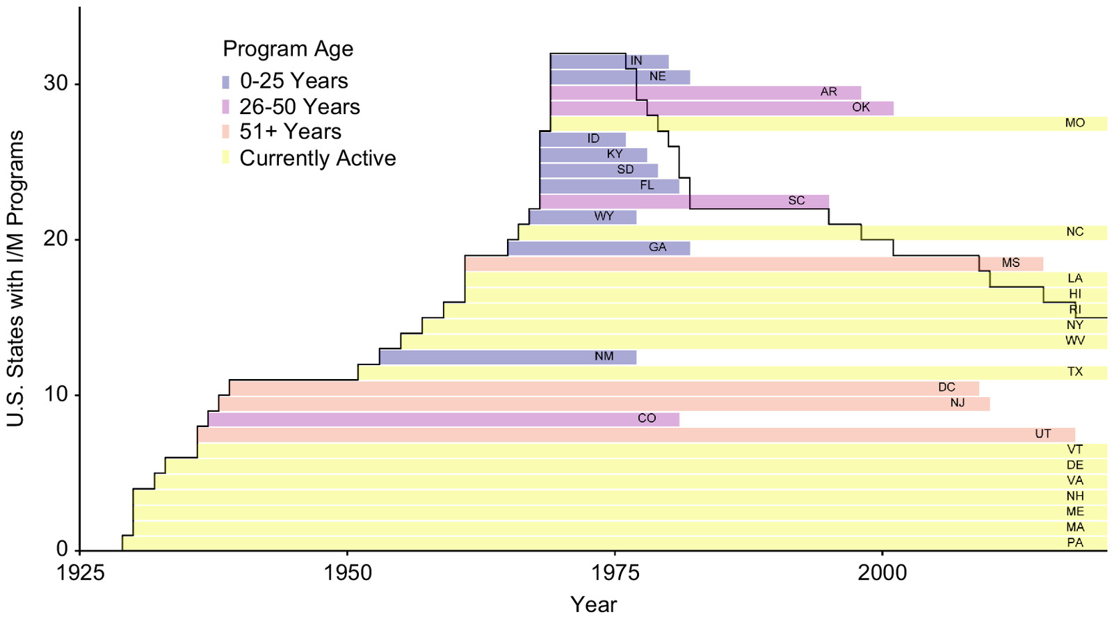
I/M programs were among the earliest strategies implemented to regulate vehicle safety in the United States. The first programs were voluntary (i.e., states recommended periodic inspections but did not mandate them). Massachusetts’ voluntary program, founded in 1926, was followed in quick succession by similar offerings in states across the eastern seaboard. The first mandatory safety I/M program was established in 1929 in Pennsylvania; this program continues to be active and is the nation’s longest running safety I/M program. After a 1968 hearing in the US Senate found that vehicle owners were incurring high costs for unsatisfactory vehicle repairs, the Motor Vehicle Information and Cost Savings Act was passed, giving the US DOT (through state agencies, if needed) the power to establish inspection stations and conduct vehicle safety inspections (Schroer and Peyton 1979). As a result, in 1973, NHTSA issued vehicle-in-use (VIU) standards, with the intention of requiring every US state to institute a safety I/M program. This rule received almost immediate pushback from the states, compelling NHTSA to weaken the VIU standards in 1976, no longer requiring mandatory inspections (Thompson 1985). As a result, while over a dozen US states established programs in the 1960s and 1970s, several of them were repealed soon after. Though not mandating I/M programs, NHTSA continues to promote safety inspections in recommendations and guidance, such as routinely published Proactive Safety Principles. Yet of the 32 active I/M programs in 1976, 18 have since been repealed, and no new programs have been established (GAO 2015). As shown in Fig. 1, only 14 US states continue to have mandatory periodic vehicle safety inspection programs in 2020.
The decline in legislative and popular support for these programs since the mid-1970s, which has led to this string of repeals, was primarily motivated by “waning public concern with highway safety” and the perception “that mechanical defects cause a small portion of” accidents (Thompson 1985, p. 696). Although there may be a perception that I/M programs are ineffective since newer vehicles rarely fail safety inspections, Peck et al. (2015) noted that this perception hinges on a significant underestimation of the number of LDVs failing safety inspections. Additionally, they argued that since inspection failure rates do not tend to zero, they are still an important means of identifying the need for, and enforcing, critical vehicle maintenance. Stakeholders across the United States continue to advocate for the elimination of I/M programs, arguing that they are expensive to consumers and cause no significant changes in rates of road accidents or fatalities. A large strand of literature contains studies that have attempted to quantify these changes. However, most of the earlier studies (discussed in what follows) have been narrowly defined—either focusing only on one region or limiting their analyses to a short time frame. Several others also used data that may now be considered outdated. The 1970s and 1980s saw the implementation of FMVSS as well as laws lowering speed limits and mandating seat-belt use, making vehicles and roads safer and noncomparable with data or analyses from earlier decades. We believe that outdated studies based on small subsets of data from many years ago are not sufficient to support current considerations of the effectiveness of I/M programs.
Literature Review
A large number of studies in the literature examined the relationship between safety inspection programs and road accident or fatality rates, but this question has rarely been explored with a panel-data approach.
Early Quantitative Analyses
One of the first data-driven analyses of the effect of I/M programs on motor accident and roadway fatalities was a time-series regression model developed by Loeb and Gilad (1984) and updated by Loeb (1990). These regression models (based on New Jersey data from 1929 to 1979) found that “vehicle inspection […] significantly reduces the number of highway fatalities” (Loeb and Gilad 1984, p. 162). A key shortcoming of these models is the likely omitted variable bias. The first model fails to control for variables such as alcohol-related accidents and driver age, both of which were shown in earlier literature to affect fatality rates (Garbacz and Kelly 1987). Furthermore, as Garbacz (1990) observed, these models also failed to account for the so-called accident price (a variable that would internalize the private cost of an accident to each driver) and that if this variable were added to the Loeb (1990) regression model, the conclusion was that I/M programs have no discernible effect. Garbacz’s assertion that private costs are a key indicator of driver propensity for risky driving (and, hence, the likelihood of being involved in an accident) builds on the findings of Peltzman (1975), who developed a time-series regression model for national fatal accident data from 1947 to 1972 and posited that wealthier drivers had a greater appetite for risk.
A meta-analysis of these early quantitative models found several inconsistencies between them (Zlatoper 1989). Specifically, Zlatoper (1989) noted that each of the discussed models uses a different set of regressors, often missing explanatory variables that other studies have found to be significant. Therefore, this makes each model by itself incomplete. Taking cognizance of the variables of significance evaluated in past studies, the regression models presented in this paper developed a more complete picture by incorporating over 30 regressors (e.g., vehicle and driver characteristics, accident site data, and demographic information), including several that reappear in key pieces of the literature. As a measure of risk appetite (and so-called accident price), our regressions control for statewide median total and disposable income.
State- and Regional-Level Models
The aforementioned regression models—with the exception of Peltzman’s (1975)—were limited to assessing data from the state of New Jersey. Similarly, several studies of I/M program effectiveness over time have been limited in geographic scope. For example, Schroer and Peyton (1979) examined an early pilot I/M program in Huntsville, Alabama, and found the accident rate for inspected vehicles to be 9.1% lower than for uninspected vehicles. However, this study was restricted to a small sample ( vehicles inspected in 1975 or 1976 and uninspected vehicles), all of which were registered in one urban area. Analyzing Texas’ inspection and accident databases for the years 2015–2017, Murphy et al. (2018) found that crashes involving vehicles with defects were 3 to 3.5 times more likely to result in a fatality than crashes involving vehicles where such a so-called contributing factor was not recorded. That result was based on analyses of the Texas Department of Public Safety’s vehicle inspection database, and its methods may therefore not be directly replicable in other jurisdictions. Hoagland and Woolley (2018) applied synthetic controls to assess the repeal (in 2010) of New Jersey’s I/M program and found no significant effect on fatality rates. The study only used data from 2000 to 2015, and its findings may not account for historical time-variate trends in vehicle safety.
Studies Applying Highway Statistics Data
Numerous studies with a national scope also exist in the literature. Based on Highway Statistics data for 1981–1993 from the Federal Highway Administration (FHWA), Merrell et al. (1999) found that inspections had no statistically significant impact on fatalities or injuries from the presence or absence of safety inspection programs. Their specification included a lagged dependent variable, and they noted that fixed-effects (FE) models may not control for serial correlation. Merrell et al. (1999) hypothesize two reasons explaining the lack of any effect—first, the behavioral offset discussed by Peltzman (1975), and second, that drivers have an incentive to properly maintain their vehicles regardless of whether or not an I/M program exists. Although FE models, such as those presented by Merrell et al. (1999), are well suited to modeling longitudinal data, their precise specifications are prone to unobserved heterogeneity and omitted variable biases; therefore, their findings are widely accepted to be correlative rather than causal. The FE regressions presented in this study are supported by a supplementary instrument variable regression to better control for these biases and better examine any causal effect of I/M programs on road fatality rates. Further, the Highway Statistics data applied in the aforementioned studies are based on representative samples and are designed only to be nationally representative (FHWA 2018). That data set is not designed to be accurate at higher resolutions.
Therefore, the application of these data for state-level analyses, as conducted by Merrell et al. (1999), may suffer from errors due to sampling biases. Based on the findings of Merrell et al. (1999), Sutter and Poitras (2002) argued that, although there is no correlation between inspections and fatality rates, the reason that I/M programs continue to exist may be explained by lobbying efforts and by so-called transaction cost inertia. However, we note that four state I/M programs have been repealed since 2002, and three of those were over 60 years old. This may indicate the presence of other factors that could counteract these effects. Poitras and Sutter (2002) used data for the years 1953–1967 and found that the presence of I/M programs had no impact on either the usage of old cars (i.e., scrappage rate) or the revenue for the automobile maintenance industry—which, they assert, shows I/M programs do not lead to improved vehicle maintenance. The data used by Poitras and Sutter (2002) represent a period during which a majority of active I/M programs were nascent; the longer-term effects of these programs may not be captured in data through 1967. Another recent national-level assessment applied text-mining tools to the NHTSA Vehicle Complaints Database from 2010 to 2016 and developed a regression that indicated that states with I/M programs had fewer vehicle complaints in the database. The NHTSA Vehicle Complaints Database includes complaints voluntarily submitted by vehicle owners regarding any defects related to “vehicles, tires, child safety seats, equipment” (NHTSA 2020b). A majority of these complaints do not relate to accidents, injury, or fatalities. Therefore, like the Highway Statistics data, this database is also prone to sampling errors and not likely an accurate representation of accident or fatality rates at the state level. As demonstrated earlier, although significant attention over time has been paid to the effects of I/M programs on safety, the majority of studies are over 20 years old, with just a few narrowly scoped studies in that time period.
International Programs
Numerous international studies have also been conducted on the effectiveness of I/M programs. A study of inspections in New Zealand found that not only were inspections effective but also that the likelihood of a vehicle being in an accident was correlated with the time since its last inspection (i.e., as the vehicle spends more time uninspected, it is increasingly likely to be involved in an accident) and that this conclusion held true regardless of vehicle age (White 1986). This finding was supported by more recent data from the case-controlled Auckland Car Crash Injury Study, which provided twice-yearly inspections and tire-pressure checks to over 500 drivers and collected data from a control group of roughly the same size that received no treatment. Over the 18-month period of analysis (1998–1999), the study concluded there was “significantly greater odds of being involved in a crash where someone was injured or killed” (Blows et al. 2003). It must be noted that these New Zealand studies, while rigorous, were based on a relatively small sample of drivers.
A control study with a much larger sample was conducted in Norway. Fosser (1992) assigned over 200,000 vehicles to one of three groups: vehicles inspected annually, vehicles inspected once in the 3-year study period, and a control group of vehicles only subjected to the existing random inspection regime. The study found—during the 3-year analysis period—no correlation between a vehicle’s propensity to be involved in an accident and which group it was in. A more recent study of Norway’s biennial inspections applied a negative binomial model and found that inspected vehicles had fewer defects and vehicles with fewer defects had lower accident rates. However, the researchers also found there to be no direct effect of inspections on accident rates (Christensen and Elvik 2007). The authors of that study hypothesized that this counterintuitive outcome might be the result of drivers who adapted their behavior to the technical condition of their vehicle or drivers who, being less concerned about safety, were more likely to drive defective cars (and these drivers would see higher accident rates regardless of the condition of their vehicle).
As demonstrated earlier, althoug significant attention over time has been paid to the effects of I/M programs on safety, the majority of studies are over 20 years old, with just a few narrowly scoped studies in that time period.
Motivation
Jurisdictions continue to debate the need for, and effectiveness of, I/M programs while relying on outdated or narrowly focused evidence in the literature. To better inform future legislation and policy development, this study aimed to develop a reproducible and data-driven analysis that applied nationally representative data over the longest possible period, to quantify the mitigating effect—if any—of safety I/M programs on motor accidents and roadway fatalities. Applying a panel of fatal accident data representing all 50 states (and the District of Columbia) over a 44-year period, we developed a FE regression to control for the potential state and time effects in order to improve the robustness of our estimates. Our specification regressed the presence of state I/M programs against adjusted roadway fatality rates while controlling for several related factors. The results obtained from the FE regression were supported by several supplementary regressions, including an instrument variable regression that relaxed the assumption that the implementation of the I/M program (i.e., the treatment) was random across states.
Contributions of This Study
Given the variation in fleet and driving characteristics between countries and regions, it is unclear whether, and to what extent, the findings of these international studies will hold true in the United States. Unlike in Europe, where I/M programs are typically administered at the national level, passenger vehicle safety inspections in the United States are based on a patchwork of state-level regulations, whereas accident and fatality rates also continue to depend on nationwide trends and federal laws. The results presented in what follows were developed from US accident and demographic data of uniform resolution (rather than sampled surveys) in all 50 states and the District of Columbia, allowing stakeholders to access relevant, national-level results instead of interpolating from regional or international studies. Rather than assessing only one state or region, the results presented in what follows indicate an average treatment effect (ATE) of I/M programs on roadway fatalities across the United States. Given the variation in demographics, fleet characteristics, and state governments, we admit it is likely that a state-by-state model would reveal heterogeneity in treatment effects between states and that exogenous variables may not fully account for these state-to-state differences. However, to facilitate comparison of effects across states, we believe it necessary to calculate an ATE. To ensure that our estimate of the ATE is unbiased (e.g., free from the influence of state-specific unobservable or omitted biases), we adjust for differences between states that are relevant for program establishment/repeal and for the outcomes in our regression specifications. It would not be possible to make these adjustments in a state-level analysis.
Regressions based on shorter time frames are also more likely to include bias in estimating any time-related effects. As discussed in the following section, the data used in this study represent the largest publicly available road fatality database in the United States; this database contains records of nearly every fatal accident that occurred anywhere in the country over a period of more than four decades.
Data
A strong quantitative assessment of US I/M programs’ impact on accidents and fatalities uses data on all road accidents (regardless of their severity) from every US state, over a long period during which subsets of statewide programs were established and repealed. This data set includes records of whether these accidents may be attributable to vehicle components or other elements that may have been remedied by a timely vehicle inspection. Additionally, consistent data that are of similar quality and resolution in each jurisdiction and over time would be critical. However, since accident data collection is typically managed by state-level DOTs, and first responders and law-enforcement agencies are managed at the city or county level, there exists neither a framework nor an incentive for the uniform collection and nationwide dissemination of data from every fatal motor accident. Although the NHTSA National Automotive Sampling System–General Estimates System (NASS-GES) may provide valuable insights at the national level, it is based on sampled data and, as such, is not designed to have meaning at the state level (NHTSA 2020c; Peck 2015). Databases maintained by state DOTs [e.g., in Texas, as described by Murphy et al. (2018)] may account for all accidents in that state, but these data are likely to vary widely in resolution and format between states. As such, a database of all motor-vehicle accidents in the United States that is uniformly resolved at the state level is not publicly available. For this reason, the models presented in this study (and those in several earlier studies, discussed in the Appendixes) have been restricted to evaluating I/M programs’ impact on fatal accidents—for which such a database is free and publicly accessible.
Fatality Analysis Reporting System
Every year, states share data with NHTSA on all police-reported fatal motor accidents in their jurisdiction through the Fatality Analysis Reporting System (FARS), which was created by an act of Congress (NHTSA 2020a). “The FARS crash data files contain more than 100 coded data elements characterizing the crash, vehicles, and people involved” (NHTSA 2010). This feature-rich data set is maintained primarily to inform regulation in Congress and at the USDOT. Although reporting data to FARS is entirely voluntary and governed by cooperative agreements, most states have regulations mandating the collection and submission of data on fatal accidents. This reporting—since 1975—has led to the development of a nationwide census of fatal accidents over the last four decades. The FARS database provides a uniform and systematic format for states to record and share fatal accident data, which is why it was selected for this study. We decide to focus on road fatality rates as our primary outcome of interest since the likelihood of reduction in fatalities is a strong element in decisions surrounding the implementation, withdrawal, or maintenance of I/M programs. Another advantage of the FARS database is that, unlike the limitations of other data sources used in previous studies, the FARS database provides feature-rich, uniform, and systematically recorded data on fatal accidents in every state and over several decades. Owing to this consistency, the models presented in what follows—in line with numerous past studies—use the FARS database to assess I/M programs’ effect on fatality rates. Although the task of collecting, collating, and submitting data to the FARS database falls on first responders and on staff at state DOTs, the process is heavily controlled by NHTSA. Summary statistics and additional information regarding the FARS data are provided in the Appendixes.
Vehicle Contributing Factors
The FARS database includes records of vehicle contributing factors, i.e., factors related to involved vehicles’ safety features that first responders may have taken the time to perceive to have led to an accident. The FARS data format allows for the optional recording of over a dozen so-called contributing factors, as listed in the Appendixes. These factors—such as low tire-tread depth or worn brakes—involve components that would typically be inspected and remedied during a periodic inspection. Fig. 2 shows the percentage of yearly fatal crashes in each state, for which at least one contributing factor was recorded in FARS between 1975 and 2017. Overall, between 1975 and 2017, at least one contributing factor was recorded in just over 3% of all fatal accidents. In theory, these data would be the most reliable indicator of the impact of I/M programs on preventing fatal accidents since a vast majority of these factors would likely have been identified and remedied during a safety inspection. Police officers who respond to fatal accidents are expected to include information on these factors in their reports. Analysts trained by NHTSA then format and record information from these reports for submission to the FARS database (NHTSA 2010). There may be evidence in the literature that these data may be underreported: Although they did not examine vehicle contributing factors specifically, Rolison et al. (2018, p. 22) found that other contributing factors (e.g., driver distraction and impairment, cell-phone use) are underreported, since the priority of responding officers at the scene of an accident is to ensure the safety of road users rather than to collect these data. This evidence is also supported by anecdotal accounts of numerous I/M program administrators. Given our belief that these data are underreported, the specifications developed in this study apply a dependent variable based on all fatal accidents, regardless of whether such a contributing factor was recorded. However, the proportion of accidents with a recorded contributing factor was included as a control to evaluate its correlation respectively with other exogenous variables and with the rate of fatalities. Additional discussion of vehicle contributing factors is provided in the Appendixes.

Furthermore, we chose not to focus our analyses on these contributing factors since, unlike the control studies conducted by Fosser (1992) and Christensen and Elvik (2007), data on defects or contributing factors are not publicly available in the United States for vehicles not involved in accidents.
Complementary Data
In addition to FARS, this analysis uses numerous other data sources, all of which are free and publicly available (FHWA 2018; US Census Bureau 2016, 2020; NCEI 2020; NCSL 2020). Further discussion of these supplementary data sources, and the regressors developed from them are presented in the following section and in Appendix IV.
Methodology
Time-Series Regression Models
The availability of longitudinal data on accidents occurring at the state level enabled us to gather information and responses to a total of 51 jurisdictions over 44 years (1975–2018). Given the large temporal span and geographical coverage of the data, we built our econometric specifications on the basis of panel data models because they allowed us to control for broader time trends and state effects across observed units (Chamberlain 1984; Hsiao 2003) that should clear our estimates from external biases unrelated to the implementation of I/M programs (e.g., improved standards, seat-belt laws) that can still impact road fatality rates. Therefore, the specifications in our analysis use both time and state FE. The decision to use panel data models is in line with the recent strands of the literature, as several recent studies discussing model and regressor specifications for the prediction of accident and fatality rates concur on the use of panel data models to assess weighted fatality rates (Stipdonk et al. 2010; Siegrist 2010; Hauer 2010; Liu et al. 2018; Chen et al. 2018; Fountas et al. 2018).
We note here that by modeling average or mean values, rather than looking at each vehicle’s inspection status during an accident, our analyses may be subject to an ecological fallacy. However, we believe that by limiting our analyses to in-state passenger vehicles, we are able to reasonably assume the inspection status of each individual vehicle and of the group as a whole, based on the inspection requirements in each state at the time of analysis. Furthermore, mean accident data are calculated based on individual-vehicle level records, and resultant errors are explicitly stated in our analyses.
Accounting for I/M Program Jurisdiction
The FARS database includes fatal road accidents of all types, including those involving commercial vehicles (e.g., buses, trucks, other commercial equipment), which are governed by safety standards and I/M programs unrelated to the LDV I/M programs that are the focus of this study. Therefore, we exclude accidents involving only other types of vehicles and accidents involving passenger vehicles as well as other types from the present analysis. This allows for models to be developed around only those vehicles that are likely covered by the I/M programs in question.
Passenger vehicle I/M programs are administered at the state level, usually by transportation agencies, which implies that the jurisdiction of each I/M program is assumed to be limited to vehicles registered in said states. However, a considerable proportion of vehicle miles (1 km = 0.62 mi) are traveled out-of-state, and as a result, vehicles may be involved in accidents outside their home state. One previous study addressed that issue by ignoring the location of the accident and developed panels based solely on vehicles’ state of registration (Hoagland and Woolley 2018), but this strategy is limited by the fact that it does not control for state-based differences across states in first-responder procedures, which can lead to biases since data collection and reporting norms can differ significantly from one state to another. This study contributes to the literature by clearing up this potential threat to estimate quality. We restrict the analysis to accidents in which all vehicles involved were registered in the state where the accidents occurred. This approach (of restricting analyses to vehicles under the jurisdiction of specific I/M programs) does not appear in recent literature, and its application to quantifying the effectiveness of I/M programs is a unique contribution of this paper. These restrictions do not impair the size of our final sample. The analysis presented here was based on over 80% of the accidents recorded in FARS data for each year over the period 1975–2018 (for Panel I, as described in what follows) and totals over 1.33 million fatal accidents. The Appendixes provide additional details on these sampling choices.
Dependent Variable
The dependent variable selected for these models was a LDV fleet size–adjusted statewide annual road fatality rate. This allowed us to uncover any links between trends in these fatality rates and the regression variables. The rate was expressed in fatalities per 100,000 registered passenger vehicles, as shown in Eq. (1). The choice to develop these models based on a fleet size–adjusted variable was made to control for the variability in per-capita vehicle ownership (i.e., population may not be an accurate measure of the number of passenger vehicles on a state’s roadways) and to simplify the interpretation of results.
(1)
Exogenous Variables
Two data panels (henceforth referred to as Panels I and II) were developed for this analysis. Each was indexed by state and year and contained the dependent variable and the treatment variable, in addition to various exogenous variables.
Panel I
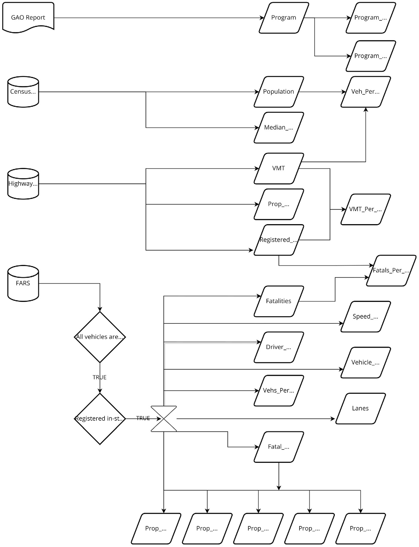
For use in the first model, a balanced panel indexed by state (50 states and the District of Columbia) and by year (1975–2018) was developed from the FARS database. These variables are listed in Table 1. The treatment variable, Program, is a Boolean variable indicating whether or not a LDV safety inspection program was active in that state during that year. The specification also includes other variables influencing the likelihood of an accident to occur (e.g., precipitation). Fig. 3 displays the raw data sources used to develop Panel I and their relationship to the regression variables.
| Variable name | Description |
|---|---|
| Program characteristics | |
| Program | Does this state have a program in this year? (, ) |
| Program_Repeal | Was this program repealed in this year? (, ) |
| Program_Ever | Did this jurisdiction ever have a program? (, ) |
| Demographics | |
| Population | Statewide population (×100,000) |
| VMT | Statewide total passenger VMT (billions) |
| Prop_Rural_VMT | Fraction of VMT estimated to be on rural roads |
| Registered_Vehicles | Number of registered passenger vehicles in state (×100,000) |
| VMT_Per_Vehicle | Statewide mean annual VMT per vehicle (×1,000 mi) |
| Veh_Per_Capita | Statewide mean number of registered passenger vehicles per capita |
| Accident data | |
| Fatal_Accidents | Total number of fatal accidents |
| Driver_Age | Mean age of all drivers involved in fatal accidents |
| Median_Income | Median statewide income |
| Fatalities | Total number of road fatalities |
| Vehicle_Age | Mean age of vehicles in fatal accidents |
| Vehicles_Per_Accident | Mean number of vehicles in each fatal accident |
| Lanes | Mean number of lanes at all accident sites |
| Speed_Limit | Mean speed limit (mi/h) at all accident sites |
| Prop_DUI | Fraction of accidents with at least one recorded DUI |
| Prop_Speeding | Fraction of accidents where at least one vehicle was speeding |
| Prop_VehCF | Fraction of accidents with at least one “vehicle contributing factor” |
| Prop_Weather | Fraction of accidents in inclement weather |
| Prop_Surface | Fraction of accidents with inclement surface conditions |
Note: VMT = vehicle miles traveled.
Panel II
Additional variables (Table 2) were collected and used in the development of a second panel (in addition to all variables included in Panel I). These variables include economic indicators. Regressions applying the within-estimator function under the assumption that the application of treatment (i.e., which states have or do not have I/M programs) is random. However, the establishment and repeal of state I/M programs are likely not random. The presence of a program in a state relies on support from legislators and state government officials. We include a binary variable indicating which political party was in power in the state legislature since the estimated treatment effect could be subject to an omitted variable bias if these political factors were not controlled for in the specification. Additionally, this party-in-power variable also allows us to test Leigh’s (1994) hypothesis that an I/M program’s strength may be politically endogenous. Further, as noted in several examples in the literature, the political party of the state government also impacts key economic indicators, including “pollution, spending, policies, and labor market outcomes” (Beland 2016, p. 2).
| Variable name | Description |
|---|---|
| Demographics | |
| GDP | Statewide average GDP per capita ($2017) |
| Pop.density | Statewide population density () |
| Disposable.income | Median statewide disposable income ($2017) |
| Driver_per_capita | Number of licensed drivers per capita |
| Democrat | Legislative party in power (, ) |
| Road characteristics | |
| Area | State area () |
| Road.length | Total length of road (mi) |
| Road.density | State road density () |
| Highway_expend_perCap | State highway expenditure ($2017) per capita |
| Precipitation | Statewide average annual precipitation (in.) |
Note: GDP = gross domestic product.
Panel II is an unbalanced panel since these data are only available for every other year between 1980 and 2006 (inclusive) and for every year in the period 2008–2017. This second set of specifications includes more variables and serves to complement Panel I. To trade off between the availability of more regressors, and this reduced frequency, we present two complementary FE regressions. Further information on data sources, variable selection, and panel development, as well as summary statistics for both panels, is presented in the Appendixes.
Variable Transformation
An inverse hyperbolic sine transformation of both the dependent and independent variables was used to improve regression performance and to facilitate easier interpretation of results. This transformation is similar to the log transform but may be used in cases where valid zeroes are present in the data. Additional discussion of this transformation may be found in Burbidge et al. (1988). When the inverse hyperbolic sine transformation is applied to both dependent and exogenous variables (Bellemare and Wichman 2020), note that regression coefficients may be interpreted as elasticities (in a similar fashion to log-log regressions).
Fixed-Effects Regressions
This study implements two main FE model specifications: Model I and Model II were based on Panel I and Panel II, respectively. Both models regress the treatment variable (i.e., the presence or absence of a state I/M program) against the dependent variable. FE models were chosen based on the result of (1) a robust Hausman specification test; and (2) an F-test (Baltagi and Bresson 2012; Hui et al. 2019). The Hausman test indicates that the rejection of the null hypothesis indicates that omitted variables may be correlated with regressors which motivated the choice of an FE model over a random effects model; and the F-Test leads to the rejection of the null hypothesis indicates the presence of fixed effects. The “within” estimator controls for omitted variable bias, with regard to any effects that do not vary over time, and are specific to individuals (in this case, states). Further, these models assume the effects are correlated with one or more regression features. The “within” estimator de-means each variable, thereby cancelling out the term corresponding to these individual effects. State effects include variations between states, which are relatively time invariant but which may account for differences in the dependent variable, e.g., road conditions and funding, climate, and the relative volume of industry and related commercial or industrial traffic. For a dependent variable (i.e., fatality rate) , as defined for a state and year , real data generation may be assumed to follow a process, as shown in Eq. (2), where represents the time-invariant effect associated with any omitted variables. The “within” estimator de-means this equation, thereby counteracting , as shown in Eq. (3):
(2)
(3)
Since the literature indicates effects both across time and states (i.e., so-called individual effect), FE Models I and II are two-way models and control for both state and time FE. By applying two-way models, we aim to control for individual and time effects. The FE models described here were developed with the plm package in R (Croissant and Millo 2008; R Core Team 2020).
We present two FE regressions. Model I was developed based on Panel I (a balanced panel for 51 jurisdictions and each year in the period 1975–2018), and Model II was developed on Panel II (which contains data for all 51 jurisdictions, but only a subset between 1975 and 2017). Panels I and II are further described in earlier sections on exogenous variables. To address any possible correlation between exogenous variables, FE Models I and II use only a subset of variables from the corresponding panels. We selected variables for each regression on the basis of variance inflation factors (VIFs), calculated for ordinary least squares (OLS) regressions for each panel, containing all exogenous variables from that panel. For Panel I, two variables—vehicle ownership per capita and proportion of driving on rural roadways—were found to have and were thus excluded from Model I. For Panel II, two iterations were conducted. Five variables with in the first regression were excluded from a second OLS regression. Only variables with a in this second iteration were included in FE Model II. The VIFs calculated from the OLS model are presented in the Appendixes. By excluding variables that do not meet the VIF threshold, the FE regressions presented here are unlikely to be affected by correlation or multicollinearity between independent variables (Mansfield and Helms 1982). Although the Boolean variable Program_Ever was included in the Model I specification, it was dropped during the regression (since it was redundant in a two-way model that controlled for both time and state).
Supplementary Regressions
Two-Stage Least-Squares Regression
A core assumption of FE specifications is that treatments (i.e., the presence or absence of the I/M program) are considered randomly distributed. In reality, the establishment or repeal of I/M programs is driven by a multitude of factors, including the affiliation and strength of state legislatures and election cycles. Shedding light on the existence and importance of these factors, Graham and Garber (1984, p. 206) argued that trying to estimate the impact of vehicle safety legislation on fatalities is rationalist, whereas driving decisions are more behavioral in nature, and that most existing literature falls into “some general pitfalls in using statistical results in policy analysis.” In agreement with Graham and Garber (1984), Leigh (1994) argued that vehicle safety must be treated as politically endogenous, specifically that the strength of vehicle safety in a state is a function of the direction and volume of lobbying for or against I/M programs in that state. After controlling for this endogenous tendency for safety in each state, Leigh (1994) found I/M programs themselves to not have any significant contribution.
Therefore, we complement the FE analysis with a two-stage least-squares (2SLS) regression to account for reverse causality and omitted variables, which may bias the FE regressions, preventing any meaningful causal inferences from being drawn. A 2SLS regression is carried out in two steps. First, the exogenous variables () are regressed against selected so-called instrument variables (). The dependent variable () is then regressed on the predicted values () from the first regression. Instrument variables are selected to satisfy two conditions; they must be correlated with the dependent variables but must not be correlated with the error term. By controlling for time-dependent omitted variable bias, the 2SLS could uncover any causal relationship between the treatment and dependent variables (James and Singh 1978). The 2SLS model presented in this study applied the same panel and set of regressors as FE Model I. Two instrument variables were selected for this regression: the third lags of the Prop_Speeding (i.e., fraction of fatal accidents involving at least one speeding vehicle) and Prop_DUI [i.e., fraction of fatal accidents involving at least one instance of driving under the influence (DUI)] variables. The authors assert that these variables fit both conditions for unbiased instruments discussed previously, specifically, that the instrument and dependent variables are correlated since high rates of speeding- and DUI-related fatal accidents will likely lead to mitigation strategies over subsequent years (such as additional law enforcement, reduced speed limits, redesigned roadways and intersections), which would in turn reduce the number of roadway fatalities. These variables were also found to reject the null hypotheses of a Sargan test (for overidentification) as well as a Durbin–Wu–Hausman test (for estimator consistency) (Sargan 1958; Patrick 2021). The 2SLS regressions were developed with the AER package in R (Kleiber and Zeileis 2008; R Core Team 2020).
Vehicle Contributing Factors Data
As discussed earlier, we believe that contributing factor data may not fully capture maintenance-related factors causing a fatal accident, especially since the effect of such factors may also be compounded by other variables (e.g., weather and surface conditions may exacerbate the effects of tires or brakes that are near or below the standards of safety). For this reason, we believe it is important to examine the ATE of I/M programs on all in-state fatal passenger vehicle accidents. We developed a modified version of Model I, regressing the exogenous variables against the proportion of fatal accidents in which a contributing factor was recorded (i.e., Prop_VehCF), as well as the raw count of fatal accidents in which such a factor was recorded, for each state in each year. Much like Model I, these regressions also used data from Panel I and applied a two-way FE regression with a ‘within’ estimator.
Results
Fixed-Effects Regressions
Table 3 presents estimates from Models I and II. The coefficient for the treatment variable is found to be negative and statistically significant in both models (respectively at the 90% and 95% levels), indicating that states with I/M programs have a lower fatality rate than those without. Model II showed a reduction in fatality rates of 5.5% (95% CI: 0.4% to 10.6%), and Model I—with fewer variables but over a longer time period—found a complementary result: Jurisdictions with I/M programs had 2.8% (90% confidence interval [CI]: 0% to 5.6%) fewer fatalities per 100,000 registered vehicles than those that did not.
| Variable | Dependent variable | |
|---|---|---|
| Fatals_Per_100k_Veha | ||
| Model I | Model II | |
| Program | (0.017)* | (0.026)** |
| Program_Repeal | (0.035) | (0.053) |
| Populationa | (0.034)*** | — |
| Driver_Agea | (0.080)*** | 0.055 (0.101) |
| Median_Incomea | 0.038 (0.078) | 0.105 (0.104) |
| Vehicle_Agea | 0.145 (0.048)*** | 0.344 (0.070)*** |
| Vehicles_Per_Accidenta | 0.523 (0.116)*** | 0.175 (0.144) |
| Lanesa | 0.032 (0.047) | (0.059)** |
| Speed_Limita | 0.119 (0.095) | 0.290 (0.131)** |
| Prop_DUIa | 0.213 (0.051)*** | 0.326 (0.076)*** |
| Prop_Speedinga | (0.043)*** | (0.055) |
| Prop_VehCFa | (0.156) | (0.242) |
| Prop_Weathera | 0.121 (0.061)** | 0.076 (0.067) |
| Prop_Surfacea | (0.097) | 0.084 (0.122) |
| Veh_Per_Capitaa | (0.084)*** | (0.106)*** |
| Prop_Rural_VMTa | — | 0.460 (0.144)*** |
| GDPa | — | 0.470 (0.073)*** |
| Highway_expend_perCapa | — | (0.020) |
| Precipitationa | — | 0.021 (0.025) |
| Democrat | — | (0.011)*** |
| 0.584 | 0.609 | |
| F-statistic | 70.291 | 38.469 |
| Observations | 2,244 | 1,224 |
Note: DUI = driving under the influence; GDP = gross domestic product; and VMT = vehicle miles traveled. *; **; and ***.
a
Inverse hyperbolic sine transformation applied to this variable.
Both models also indicate that fatality rates are negatively correlated with mean vehicle age, which corroborates findings in the literature that crashes involving older vehicles are more likely to result in fatalities. The models also indicate a negative correlation between the accident rate and the number of passenger vehicles registered per capita. Model II also found two of the additional demographic variables to be statistically significant—the statewide gross domestic product (GDP) and the political party in power at the state level. The sources and means of calculating these variables are presented in Appendix IV. Further, the results are robust to the inclusion of the party-in-power controls, which indicates that our conclusions are not impaired by nonrandomness or omitted variable bias. Neither Model I nor Model II found the proportion of accidents with a recorded vehicle contributing factor to be significant.
Supplementary Regressions
Two-Stage Least-Squares Regression
Table 4 shows results from the 2SLS regressions. Estimates corroborate the previous findings from the FE models because they indicate that there exists a statistically significant negative relationship between the presence of an I/M program, and the road fatality rate.
| Variable | Dependent variable |
|---|---|
| Fatals_Per_100k_Veha | |
| Program | (0.11)*** |
| Program_Repeal | (0.06)*** |
| Populationa | (0.04)*** |
| Driver_Agea | (0.12) |
| Median_Incomea | (0.09) |
| Vehicle_Agea | 0.17 (0.05)*** |
| Vehicles_Per_Accidenta | 0.58 (0.13)*** |
| Lanesa | 0.02 (0.05) |
| Speed_Limita | 0.25 (0.11)** |
| Prop_VehCFa | (0.18) |
| Prop_Weathera | 0.28 (0.08)*** |
| Prop_Surfacea | (0.11)** |
| Veh_Per_Capitaa | (0.10)*** |
| 0.88 | |
| Number of observations | 2,244 |
| Diagnostic test statistics | |
| Weak instruments | 26.447*** |
| Durbin–Wu–Hausman | 9.379** |
| Sargan | 10.695** |
Note: **; and ***.
a
Inverse hyperbolic sine transformation applied to this variable.
Vehicle Contributing Factors Data
The results for the regression against the proportion and count of fatal accidents with a recorded vehicle contributing factor are presented in Table 5. We note that the significance of these findings is diminished by the models’ low coefficient of determination (), which was in both cases. A low value indicates that the treatment variable likely explains only a small portion of any change in the dependent variables. With that in mind, these results appear to show a statistically significant negative correlation between the treatment variable (presence of an I/M program) and the dependent variables (proportion or count of fatal accidents with a vehicle contributing factor), which indicates that the presence of an I/M program reduces the proportion of fatal accidents with a contributing factor (which only account for about 3% of all accidents) by 0.7% (95% CI: 0.5% to 0.9%) while controlling for other exogenous variables. At first glance, it may appear from these regressions that the effect of I/M programs on the number of fatal accidents with a contributing factor is substantial (36%), supporting the hypothesis that the effectiveness of I/M programs in specifically targeting fatal accidents that involve such a contributing factor. However, we must interpret these results in the context that only about 3% of all fatal accidents have a recorded contributing factor. The reduction in the proportion of accidents with a recorded factor by 0.7% (of that 3%) is therefore a very small number of fatal accidents. For example, in 2018, 41 states had fewer than 25 fatal accidents with a recorded vehicle contributing factor. Based on the regression estimates, this would correspond to an estimated reduction (in the number of fatal accidents) of zero. Overall, given the low and the small effect size, we conclude that, based solely on the data currently available, no ATE of I/M programs on the proportion or number of fatal accidents involving a contributing factor can be established.
| Variable | Dependent variable | |
|---|---|---|
| Fatal accidents with contributing factor | ||
| Proportiona | Counta | |
| Program | (0.002)*** | (0.081)*** |
| Program_Repeal | (0.005) | (0.171) |
| Populationa | (0.005) | 0.969 (0.170)*** |
| Driver_Agea | (0.011) | (0.385) |
| Median_Incomea | 0.010 (0.011) | 3.059 (0.375)*** |
| Vehicle_Agea | 0.036 (0.007)*** | 0.667 (0.230)*** |
| Vehicles_Per_Accidenta | (0.016) | (0.559) |
| Lanesa | (0.006)** | (0.225)*** |
| Speed_Limita | (0.013) | 1.108 (0.456)** |
| Prop_DUIa | 0.023 (0.007) | 0.256 (0.245)*** |
| Prop_Speedinga | 0.013 (0.006)** | 1.724 (0.207)*** |
| Prop_Weathera | 0.009 (0.009) | 0.188 (0.296) |
| Prop_Surfacea | 0.022 (0.013)* | 0.802 (0.466)* |
| Veh_Per_Capitaa | (0.014)** | 1.071 (0.483)** |
| Fatals_Per_100k_Vehiclesa | (0.003) | 0.254 (0.104)** |
| Observations | 2,244 | 2,244 |
| 0.038 | 0.096 | |
| F-statistic | 5.667 | 15.172 |
Note: DUI = driving under the influence. *; **; and ***.
a
Inverse hyperbolic sine transformation applied to this variable.
Discussion and Conclusions
Panel data model results provide strong evidence that jurisdictions experience lower road fatality rates due to the presence of an active safety I/M program for passenger vehicles. FE Models I and II showed a negative correlation between the presence of state I/M programs and the fleet-adjusted fatality rate: Model II had the more statistically robust result, likely because of the additional control variables. This specification showed the average treatment effect—i.e., the average reduction in fatality rates between 1980 and 2017 for states with I/M programs in comparison to those without—of 5.5% (95% CI: 0.4% to 10.6%). Model I, which has fewer control variables but applies the specification across all years from 1975 to 2018, shows a complementary result that supports the findings of Model II. As per Model I, states with I/M programs were found to have 2.8% fewer fatalities (90% CI: 0% to 5.6%) over the period of analysis.
The existence of a statistically significant, negative ATE is further supported by the value of the 2SLS regression estimates. The treatment variable coefficient is (95% CI: to ), which is of a significantly larger magnitude than the corresponding coefficients in FE Models I and II. This indicates that omitted variable bias in the FE models’ error terms causes those models to underestimate the reduction in the fatality rate in jurisdictions with active I/M programs. Further, the application of statistically robust instruments (as verified by the Sargan and Durbin–Wu–Hausman tests) indicate that the 2SLS models control for both omitted variable bias and any effect of reverse causality on the FE model errors. The authors argue that a statistically significant coefficient for the treatment variable in the 2SLS specification is thus an indicator of causality—a negative coefficient (with 95% confidence) implies that the presence of state safety inspection programs likely causes a measurable and significant reduction in the number of roadway fatalities per 100,000 registered passenger vehicles in the state. Our results are also corroborated by numerous examples in the historical literature that show a negative effect of I/M program presence on fatality rates: Loeb and Gilad (1984) found that in New Jersey alone, I/M programs mitigated over 300 fatalities () annually, and in the same state, Loeb (1990) showed that I/M programs caused 2.86 fewer fatalities per 100 million vehicle miles traveled (VMT). More recently, Das et al. (2019, p. 10) found that “states with inspection anticipate a smaller number of monthly vehicle complaints and complaint-induced crashes than the states without inspection.”
Influence of Vehicle, Infrastructure, and Traffic Characteristics
Several other regression variables were found to have a statistically significant correlation with the fatality rate. Models I and II found the mean age of vehicles involved in accidents to be positively correlated with the fatality rate. This finding is supported by studies in the literature showing that, given that an accident occurs, occupants of older vehicles are more likely to be fatally injured (O’Donnell and Connor 1996; Martin and Lenguerrand 2008). Both FE regressions also found the proportion of fatal accidents involving DUI to have a significant positive correlation with the dependent variable. This may be attributable to the fact that drunk drivers tend to drive more aggressively: Zador et al. (2000) found that “the relative risk of involvement in a fatal vehicle crash increased steadily” as driver blood-alcohol content increased.
Model I indicates an inverse relation between fatality rates and median driver age—supporting several similar findings in the literature (McCartt et al. 2009). Model I also assigned negative coefficients for the variable corresponding to the proportion of fatal accidents where speeding was recorded. Although the analyses presented here do not include a means to assess the reason behind this relationship, one potential explanation may come from evidence that points to the idea that speeding-related crashes tend to involve single vehicles with a single occupant, in constrast to accidents with multiple fatalities, which are more commonly attributable to other causes (Høye 2020).
Both models indicated that states with more registered passenger vehicles per capita had a lower fatality rate. This relationship has been explored extensively in the literature. Smeed (1949) first showed how increased traffic density would tend to decrease the number of roadway fatalities per vehicle (Oppe 1991; Ross 1985). Model I also indicated a significant negative effect of state population, suggesting that states with higher populations may have fewer road accidents per registered passenger vehicle. Further analyses are warranted to fully explain these correlations. However, the authors posit that this may be due to a concentration of urban centers in states with higher populations, where vehicle density is higher, in addition to fewer rural miles driven per capita.
With respect to additional demographic variables, Model II found there to be more road fatalities in states where a greater fraction of road miles were traveled on rural roads—in keeping with most similar studies in the literature (Peltzman 1975; Zlatoper 1989; Merrell et al. 1999)—and in states with a lower GDP (supporting the so-called Peltzman effect hypothesis). The positively correlated GDP (and the positively correlated median household income) aligns with findings in the literature that higher-income drivers are less likely to drive defensively and therefore more likely to be involved in accidents (Shinar et al. 2001; Males 2009). The positive coefficients may also be caused by a positive correlation between GDP and recreational travel (McMullen and Eckstein 2012). Increased travel, especially long-distance travel and driving on rural roads, would increase the number of fatal accidents. Model II also found a statistically significant relationship between the party in power in a state legislature (i.e., the Dem variable) and the adjusted roadway fatality rate. This party-in-power variable also allows us to test Leigh’s hypothesis that I/M program so-called strength may be politically endogenous (Leigh 1994). Further, as noted in several examples in the literature, the political party of state governments also impacts key economic indicators, including “pollution, spending, policies, and labor market outcomes” (Beland 2016, p. 2).
Vehicle Contributing Factors
It bears noting that neither regression found the proportion of fatal accidents where a contributing factor was recorded to be a significant predictor of accident rates—further supporting the hypothesis that these data may not be complete, as discussed earlier.
The supplementary regression developed to further examine this relationship (Table 5) showed a negative correlation between the treatment variable and fatal accidents involving a vehicle contributing factor. However, the regression has a low coefficient of determination, implying that the presence or absence of I/M programs and other exogenous variables still do not explain most of the variation in the number or proportion of these accidents with a recorded contributing factor. Since I/M programs are designed to address these factors, the weak treatment effect shown in this regression may appear to contradict the main finding of the other FE specifications presented. Although this dichotomy merits further investigation, we hypothesize that it may be explained by the lack of sufficiently high-resolution data (especially when compared to the variables and data sets used for Models I and II) on vehicle contributing factors in fatal accidents. Further, we hypothesize that I/M programs affect fatal accidents where—even though no vehicle contributing factor was recorded—the effect of subpar maintenance may have been compounded by factors such as road or weather conditions.
The relationship between I/M programs and vehicle maintenance, as well as between vehicle maintenance and accident rates in the United States, needs to be further examined. Unlike the randomized trials conducted in Norway by Fosser (1992) or Christensen and Elvik (2007), this study relied on fatal accident data and so could not control for the effect of inspection and maintenance programs on those vehicles that were not involved in a fatal accident. Data on vehicle maintenance and defects are not widely available in the United States, except for vehicles appearing in the FARS database.
Policy Implications and Scope for Future Work
Our results affirm—based on data from 50 states and the District of Columbia over a 44-year period—that I/M programs have a negative and causal relationship with roadway fatalities and that these programs are effective in their stated aim of mitigating roadway fatalities. In this paper, we choose not to comment on the financial cost of I/M program administration or on the potential public cost savings from mitigated accidents and fatalities. Though acknowledging these to be important factors, we argue that legislative bodies must consider the reduction in fatalities as a statistically significant benefit resulting from inspections when debating the establishment or repeal of state safety I/M programs.
The findings of this study are limited to fatal accidents, which comprise about 0.5% of all road accidents occurring in the United States each year (NHTSA 2020c). Based solely on the analyses presented here, no inferences may be made about the impact of I/M programs on less severe motor accidents; however, Blows et al. (2003) showed that changes in the rate of all motor accidents are of the same order as changes in the rate of fatal accidents. We posit that safety inspections will only become more important as advanced driver assistance systems (ADAS) and autonomous vehicle (AV) technology become more prevalent, and although several international jurisdictions have already adapted safety inspections to include testing and calibrating ADAS systems, they have not yet been applied in the United States (Bellon 2020). Future analyses could consider the vehicle-level differences in the availability of safety features and how they may help to contribute to highway safety along with I/M programs.
Appendix I. List of Abbreviations
Table 6 lists the abbreviations used in this paper.
| Abbreviation | Definition |
|---|---|
| 2SLS | Two-stage least-squares (regression) |
| ADAS | Advanced driver-assistance systems |
| ATE | Average treatment effect |
| AV | Autonomous vehicle |
| BTS | (US) Bureau of Transportation Statistics |
| CDC | US Centers for Disease Control |
| DOT | (State) Department of Transportation |
| DUI | Driving under the influence (of alcohol, drugs, for example) |
| EPA | (US) Environmental Protection Agency |
| FARS | Fatality Analysis Reporting System |
| FE | Fixed effects |
| FHWA | (US) Federal Highway Administration |
| FMVSS | Federal Motor Vehicle Safety Standards |
| GAO | (US) Government Accountability Office |
| I/M program | (Vehicle) inspection and maintenance program |
| NASS-GES | National Automotive Sampling System–General Estimation System |
| NCEI | National Centers for Environmental Information |
| NHTSA | National Highway Traffic Safety Administration |
| NOAA | National Oceanic and Atmospheric Administration |
| PennDOT | Pennsylvania Department of Transportation |
| USDOT | US Department of Transportation |
| VIF | Variance inflation factor |
| VIU | Vehicle-in-use (standard) |
| VMT | Vehicle miles traveled (usually annual) |
Appendix II. FARS Data Summaries
Table 7 lists the count of fatal accidents and road fatalities recorded in FARS each year from 1975 to 2018.
| Year | Total | Passenger, registered in state | ||||
|---|---|---|---|---|---|---|
| Accidents | Vehicles | Fatalities | Accidents | Vehicles | Fatalities | |
| 1975 | 39,161 | 55,534 | 44,525 | 32,346 | 41,926 | 36,998 |
| 1976 | 39,747 | 56,084 | 45,523 | 32,664 | 42,132 | 37,677 |
| 1977 | 42,211 | 60,516 | 47,878 | 34,252 | 44,509 | 39,110 |
| 1978 | 44,433 | 64,144 | 50,331 | 36,077 | 47,036 | 41,163 |
| 1979 | 45,223 | 64,762 | 51,093 | 36,429 | 47,129 | 41,529 |
| 1980 | 45,284 | 63,485 | 51,091 | 36,266 | 46,322 | 41,307 |
| 1981 | 44,000 | 62,699 | 49,301 | 35,253 | 45,708 | 39,795 |
| 1982 | 39,092 | 56,455 | 43,945 | 31,201 | 40,138 | 35,356 |
| 1983 | 37,976 | 55,106 | 42,589 | 30,220 | 38,992 | 34,181 |
| 1984 | 39,631 | 57,972 | 44,257 | 31,373 | 40,687 | 35,326 |
| 1985 | 39,196 | 58,271 | 43,825 | 31,008 | 40,830 | 34,884 |
| 1986 | 41,090 | 60,792 | 46,087 | 33,019 | 43,446 | 37,339 |
| 1987 | 41,438 | 61,836 | 46,390 | 33,527 | 44,508 | 37,789 |
| 1988 | 42,130 | 62,703 | 47,087 | 34,410 | 45,640 | 38,780 |
| 1989 | 40,741 | 60,870 | 45,582 | 33,498 | 44,913 | 37,715 |
| 1990 | 39,836 | 59,292 | 44,599 | 32,667 | 43,541 | 36,748 |
| 1991 | 36,937 | 54,795 | 41,508 | 30,312 | 40,292 | 34,278 |
| 1992 | 34,942 | 52,227 | 39,250 | 28,916 | 38,888 | 32,689 |
| 1993 | 35,780 | 53,777 | 40,150 | 29,648 | 39,636 | 33,401 |
| 1994 | 36,254 | 54,911 | 40,716 | 29,848 | 40,399 | 33,706 |
| 1995 | 37,241 | 56,524 | 41,817 | 30,795 | 41,817 | 34,745 |
| 1996 | 37,494 | 57,347 | 42,065 | 31,153 | 42,361 | 35,113 |
| 1997 | 37,324 | 57,060 | 42,013 | 31,061 | 42,284 | 35,154 |
| 1998 | 37,107 | 56,922 | 41,501 | 30,722 | 42,124 | 34,481 |
| 1999 | 37,140 | 56,820 | 41,717 | 30,813 | 42,086 | 34,687 |
| 2000 | 37,526 | 57,594 | 41,945 | 31,076 | 42,441 | 34,920 |
| 2001 | 37,862 | 57,918 | 42,196 | 31,290 | 42,663 | 35,083 |
| 2002 | 38,491 | 58,426 | 43,005 | 31,690 | 43,033 | 35,610 |
| 2003 | 38,477 | 58,877 | 42,884 | 31,494 | 42,836 | 35,259 |
| 2004 | 38,444 | 58,729 | 42,836 | 31,288 | 42,384 | 35,027 |
| 2005 | 39,252 | 59,495 | 43,510 | 31,489 | 42,316 | 35,151 |
| 2006 | 38,648 | 58,094 | 42,708 | 31,040 | 41,179 | 34,525 |
| 2007 | 37,435 | 56,253 | 41,259 | 29,900 | 39,715 | 33,160 |
| 2008 | 34,172 | 50,660 | 37,423 | 26,961 | 35,296 | 29,693 |
| 2009 | 30,862 | 45,540 | 33,883 | 24,725 | 32,487 | 27,330 |
| 2010 | 30,296 | 44,862 | 32,999 | 24,188 | 31,715 | 26,544 |
| 2011 | 29,867 | 44,119 | 32,479 | 23,738 | 31,032 | 25,973 |
| 2012 | 31,006 | 45,960 | 33,782 | 24,765 | 32,271 | 27,151 |
| 2013 | 30,202 | 45,101 | 32,893 | 24,111 | 31,590 | 26,426 |
| 2014 | 30,056 | 44,950 | 32,744 | 24,089 | 31,651 | 26,391 |
| 2015 | 32,538 | 49,478 | 35,484 | 26,135 | 34,778 | 28,703 |
| 2016 | 34,748 | 52,714 | 37,806 | 27,768 | 37,178 | 30,408 |
| 2017 | 34,247 | 52,645 | 37,133 | 27,317 | 36,732 | 29,804 |
| 2018 | 33,654 | 51,872 | 36,560 | 26,721 | 35,929 | 29,230 |
Table 8 shows these same data, by state, for 2018 (the most recent year for which FARS data are available at the time of writing).
| State (FIPS) | Total | Passenger, registered in state | ||||
|---|---|---|---|---|---|---|
| Accidents | Vehicles | Fatalities | Accidents | Vehicles | Fatalities | |
| Alabama (01) | 876 | 1,321 | 953 | 714 | 942 | 785 |
| Alaska (02) | 69 | 104 | 80 | 57 | 74 | 67 |
| Arizona (04) | 916 | 1,404 | 1,010 | 573 | 795 | 643 |
| Arkansas (05) | 472 | 735 | 516 | 356 | 478 | 389 |
| California (06) | 3,259 | 4,986 | 3,563 | 2,701 | 3,708 | 2,989 |
| Colorado (08) | 588 | 897 | 632 | 471 | 608 | 507 |
| Connecticut (09) | 276 | 417 | 294 | 209 | 279 | 224 |
| Delaware (10) | 104 | 168 | 111 | 76 | 99 | 78 |
| District of Columbia (11) | 30 | 44 | 31 | 12 | 13 | 12 |
| Florida (12) | 2,915 | 4,564 | 3,133 | 2,395 | 3,246 | 2,595 |
| Georgia (13) | 1,407 | 2,165 | 1,504 | 1,129 | 1,495 | 1,214 |
| Hawaii (15) | 110 | 157 | 117 | 90 | 110 | 97 |
| Idaho (16) | 212 | 316 | 231 | 148 | 186 | 160 |
| Illinois (17) | 948 | 1,481 | 1,031 | 751 | 1,040 | 819 |
| Indiana (18) | 774 | 1,218 | 858 | 625 | 841 | 694 |
| Iowa (19) | 291 | 469 | 318 | 221 | 290 | 244 |
| Kansas (20) | 366 | 568 | 404 | 266 | 343 | 296 |
| Kentucky (21) | 664 | 1,033 | 724 | 542 | 713 | 597 |
| Louisiana (22) | 716 | 1,070 | 768 | 599 | 777 | 645 |
| Maine (23) | 128 | 179 | 137 | 99 | 121 | 105 |
| Maryland (24) | 474 | 741 | 501 | 368 | 490 | 391 |
| Massachusetts (25) | 343 | 491 | 360 | 277 | 347 | 291 |
| Michigan (26) | 905 | 1,480 | 974 | 778 | 1,115 | 842 |
| Minnesota (27) | 349 | 538 | 381 | 286 | 385 | 316 |
| Mississippi (28) | 597 | 898 | 664 | 497 | 629 | 554 |
| Missouri (29) | 848 | 1,344 | 921 | 644 | 888 | 709 |
| Montana (30) | 168 | 214 | 182 | 123 | 146 | 134 |
| Nebraska (31) | 201 | 353 | 230 | 154 | 235 | 177 |
| Nevada (32) | 300 | 452 | 330 | 223 | 302 | 245 |
| New Hampshire (33) | 134 | 193 | 147 | 92 | 116 | 104 |
| New Jersey (34) | 525 | 782 | 564 | 412 | 539 | 446 |
| New Mexico (35) | 350 | 520 | 391 | 240 | 302 | 267 |
| New York (36) | 889 | 1,291 | 943 | 701 | 891 | 753 |
| North Carolina (37) | 1,321 | 2,065 | 1,437 | 1,100 | 1,514 | 1,207 |
| North Dakota (38) | 95 | 144 | 105 | 63 | 77 | 72 |
| Ohio (39) | 996 | 1,576 | 1,068 | 822 | 1,124 | 887 |
| Oklahoma (40) | 603 | 975 | 655 | 466 | 658 | 513 |
| Oregon (41) | 450 | 665 | 506 | 298 | 373 | 333 |
| Pennsylvania (42) | 1,103 | 1,686 | 1,190 | 873 | 1,170 | 946 |
| Rhode Island (44) | 56 | 82 | 59 | 35 | 40 | 35 |
| South Carolina (45) | 970 | 1,475 | 1,037 | 799 | 1,052 | 852 |
| South Dakota (46) | 110 | 148 | 130 | 82 | 97 | 102 |
| Tennessee (47) | 974 | 1,518 | 1,041 | 757 | 1,041 | 812 |
| Texas (48) | 3,305 | 5,222 | 3,642 | 2,690 | 3,713 | 2,994 |
| Utah (49) | 237 | 376 | 260 | 175 | 242 | 194 |
| Vermont (50) | 60 | 86 | 68 | 47 | 58 | 52 |
| Virginia (51) | 778 | 1,154 | 820 | 627 | 813 | 661 |
| Washington (53) | 497 | 762 | 546 | 403 | 553 | 449 |
| West Virginia (54) | 265 | 409 | 294 | 192 | 249 | 214 |
| Wisconsin (55) | 530 | 799 | 588 | 408 | 548 | 457 |
| Wyoming (56) | 100 | 137 | 111 | 55 | 64 | 61 |
Note: FIPS = Federal Information Processing Standards.
Appendix III. Vehicle Contributing Factors
The FARS database includes fields for vehicle contributing factors, which are intended to record any factors of vehicle maintenance or failure that might have contributed to the fatal accident. Table 9 lists contributing factors that may be recorded in FARS. When examining individual factors, it is generally true that tires are the most commonly recorded factor throughout the data set. However, in any given year, there is a range across states in the percentage of vehicles recorded to have each type of contributing factor.
| Contributing factor | FARS data code | ||
|---|---|---|---|
| 1975–1981 | 1982–2009 | 2010–2017 | |
| Tires | 1 | 1 | 1 |
| Brake system | 2 | 2 | 2 |
| Steering system | 3 | 3 | 3 |
| Suspension | 4 | 4 | 4 |
| Power train | 5 | 5 | 5 |
| Exhaust | 6 | 6 | 6 |
| Headlights | 7 | 7 | 7 |
| Signal lights | 8 | 8 | 8 |
| Other lights | 9 | 9 | 9 |
| Mirrors | 11 | 11 | 12 |
| Wipers | 12 | 12 | 10 |
| Body | 14 | 14 | 14 |
| Trailer hitch, safety chains | 15 | 15 | 15 |
| Wheels | 1 | 16 | 11 |
| Safety systems | — | 17, 19 | 16 |
| Other vehicle defects | — | 10, 13,18 | 17, 97 |
Nationwide, states recorded anywhere between zero and 3.5% of fatal accidents in their jurisdiction that year to include at least one vehicle with tires as a contributing factor, with a median value of just over 1% of fatal accidents (involving in-state passenger vehicles) in each state. Fig. 4 shows this variation (in percentage of accidents with a recorded vehicle contributing factor) across the fifty states and the District of Columbia for the year 2018. There is a large variation not only across states but also within states over time. Based on evidence in the literature, it is likely that these contributing factors are underreported (Rolison et al. 2018).

More recent FARS data contain a variable called Critical Event–Precrash (NHTSA 2022). This field records the logistical cause of a crash (e.g., vehicle lost control) or the location and circumstances where a crash occurred (e.g., “this vehicle was turning right,” “other motor vehicle/pedestrian on road”). Although these fields are useful in better understanding an accident, the critical events are all potentially equally impacted by safety I/M programs and as such not directly related to the research question we are asking. In addition, the Critical Event–Precrash field was only introduced into FARS in 2010; therefore, it would be impossible to conduct a longitudinal analysis across the entire FARS data set (1975–2019) that we used in applying this variable. We argue that the importance of this long-term view far outweighs any benefit this variable may provide.
Appendix IV. Panel Development
Regressors
Data from FARS (which has a unique record for each fatal accident and for each involved vehicle) and other sources were used to develop regression variables corresponding to each instance of the dependent variable (i.e., statewide, annual means for each of 50 states, for each year from 1975 to 2018). An inverse hyperbolic sine transformation was applied to the dependent and independent variables, allowing for easier interpretation of results.
Mean Vehicle and Driver Ages
FARS records the model year for each vehicle involved in a fatal accident; the age of these at the time of the accident was calculated using Eq. (4). FARS also records the age of the driver (and passengers) of each vehicle. One regression variable was developed by calculating the mean age of all vehicles involved in fatal accidents in a state for each year. A second regression variable corresponds to the mean age of the drivers of these vehicles
(4)
Number of Roadway Lanes at Accident Site
A regression variable was developed by calculating the mean number of roadway lanes at the accident site for all fatal accidents in a state for each year. This variable controls for any potential difference between accident rates on higher- and lower-throughput roadways.
Median Income
For each year from 1975 to 2018, a regression variable was developed that corresponded to the statewide median household income as a fraction of nationwide annual household income for that year (as estimated by the US Census Bureau) (US Census Bureau 2016). The variable was adjusted to the nationwide median [as shown in Eq. (5)] in order to control for changes to median income nationwide over time
(5)
Vehicle Miles Traveled and Roadway Types
The USDOT’s Highway Statistics estimates the average number of vehicle miles traveled (VMT) by passenger vehicles, on each type of roadway (rural/urban, highway/city), in each state (FHWA 2018). Two regression variables were developed from these data. First, a variable corresponding to the estimated VMT per vehicle for each state–year pair was developed. Second, an estimate of the fraction of these VMT traveled on rural roads, by state and by year, was developed in order to control for the known increase in likelihood of accidents and fatalities on rural roads.
Vehicle Contributing Factors
A regression variable was developed to represent the proportion of fatal accidents for each year in a state where at least one such contributing factor (as described in what follows and in the Appendixes) was recorded in FARS for any of the vehicles involved.
DUI, Speeding, and Inclement Weather
The FARS records for each accident also reveal the weather conditions at the time of a given accident, in addition to whether a driver was speeding or whether any involved drivers were identified as having been DUI of alcohol or drugs. A regression variable was developed for each of these three sets of factors—speeding, inclement weather, and DUI—corresponding to the the proportion of fatal accidents for each year in a state where these factors were recorded for any of the vehicles involved.
I/M Program Presence and Repeal
A binary variable for each state–year combination was developed that corresponded to the presence or absence of I/M programs in that state for that year, as described in Eq. (6) (GAO 2015, Appendix I). A value of 1 indicates that an I/M program was present, whereas 0 indicates that it was absent. Similarly, a binary variable corresponding to program repeal was introduced [as in Eq. (7)]. An additional dummy control variable was introduced to distinguish two groups of states—those 31 that had an I/M program at any time during the analysis period and those 29 that never did. In all panel data specifications with both state and time effects, this variable was aliased and, hence, dropped in the regression analyses
(6)
(7)
Road Length
Data were available from 1980 to 2018 from FHWA in miles in each state (FHWA 2018). The variable road density was calculated by dividing public road length by state area.
Area and Density
The total area of each state was available from the US Census Bureau. The road density and population density were calculated by dividing the population and road length by the total area.
State Highway Expenditure
Data were available from the US Census Bureau for 1977 to 2017. The data were adjusted for inflation to 2017 rates. State highway expenditures were divided by the state population to arrive at the variable highway expenditures per capita. State GDP Per Capita Real GDP by State in chained 1997 million US dollars was available from 1977 to 1997 and also from 1997 to 2018 in chained 2012 million dollars. These were adjusted to 2017 current dollars and included as the variable GDP Per Capita.
State Legislature Political Party
The political party of the state legislature was available at the National Conference of State Legislatures from 1978 to 2018 (NCSL 2020). From 1978 to 2008, only data for even years were available, and data for the District of Columbia were also only available after 2009. The dummy variable state legislature (Democratic) was formulated using these data. The case where the state legislature was split, or in the case of Nebraska, which has a nonpartisan legislature, the variable is set to 0.
Licensed Drivers
The number of licensed drivers per state was available from FHWA from 1960 to 2018 (FHWA 2018). The number of drivers divided by state population was used as the variable drivers per capita.
Precipitation
Precipitation in each state from 1895 to 2020 was available from the National Centers for Environmental Information, so data were taken from 1967 to 2018 (NCEI 2020). For Hawaii, state average data were not available, so data for Honolulu International Airport were used as a proxy. Precipitation data are in inches (1 in. = 2.54 cm) per year.
Data from Commercial and Out-of-State Vehicles
As discussed in the “Methodology” section, only a subset of FARS data was included in these analyses. Specifically, accidents where one or more of the vehicles involved were either registered outside the state where the accident occurred or were not passenger vehicles (as recorded in FARS) were excluded. Fig. 5(c) shows that despite these restrictions, the analysis was built on over 81% of all available data in 2019. As shown in Fig. 6, over 80% of accidents from FARS data were included in the analysis for each year in the period 1975–2019, totaling over 1.33 million fatal accidents.

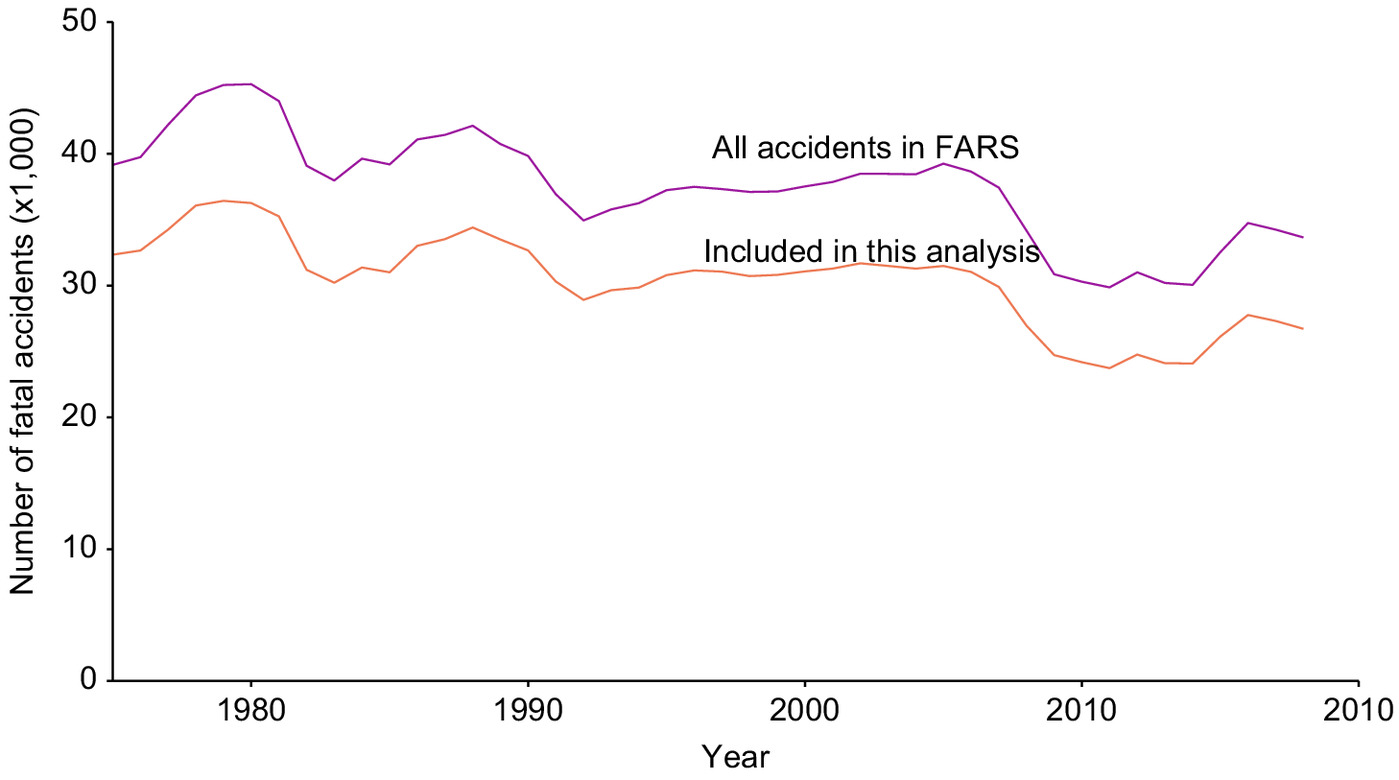
Appendix V. Summary Statistics, Data Panels
Tables 10 and 11 describe the data panels used for FE Models I and II, respectively. The first panel (from Table 10) was also used for all supplementary modeling.
| Variable | Minimum | Maximum | Mean | Standard deviation | Median |
|---|---|---|---|---|---|
| Program | 0 | 1 | 0.412 | 0.492 | 0 |
| Program_Repeal | 0 | 1 | 0.008 | 0.087 | 0 |
| Program_Ever | 0 | 1 | 0.627 | 0.484 | 1 |
| Population () | 376.170 | 39,557.045 | 5,313.190 | 5,948.093 | 3,591.057 |
| VMT (million) | 2,527 | 348,432 | 47,161.525 | 51,583.483 | 32,178 |
| Prop_Rural_VMT | 0 | 0.858 | 0.457 | 0.188 | 0.470 |
| Registered_Vehicles () | 142.717 | 20,037.727 | 2,470.443 | 2,745.115 | 1,752.886 |
| Fatal_Accidents | 3 | 4,104 | 595.928 | 625.827 | 444 |
| Driver_Age | 26.500 | 54.674 | 38.501 | 3.548 | 38.685 |
| Median_Income | 0.603 | 1.487 | 0.995 | 0.159 | 0.979 |
| Fatalities | 4 | 4,631 | 668.600 | 704.045 | 498.500 |
| Vehicle_Age | 3.024 | 15.603 | 9.184 | 1.956 | 8.905 |
| Vehicles_Per_Accident | 1 | 1.605 | 1.299 | 0.071 | 1.303 |
| Lanes | 1.939 | 4.857 | 2.364 | 0.315 | 2.299 |
| Speed_Limit | 25 | 62.567 | 47.283 | 5.202 | 48.091 |
| Prop_DUI | 0 | 0.712 | 0.370 | 0.107 | 0.367 |
| Prop_Speeding | 0 | 0.685 | 0.303 | 0.102 | 0.301 |
| Prop_VehCF | 0 | 0.224 | 0.025 | 0.028 | 0.018 |
| Prop_Weather | 0 | 1 | 0.163 | 0.092 | 0.148 |
| Prop_Surface | 0 | 0.578 | 0.195 | 0.076 | 0.190 |
| VMT_Per_Vehicle | 9,414.072 | 72,133.592 | 20,571.154 | 7,393.444 | 18,903.095 |
| Veh_Per_Capita | 0.129 | 0.740 | 0.469 | 0.089 | 0.479 |
Note: DUI = driving under the influence; and VMT = vehicle miles traveled.
| Variable | Minimum | Maximum | Mean | Standard deviation | Median |
|---|---|---|---|---|---|
| Program | 0 | 1 | 0.382 | 0.486 | 0 |
| Program_Repeal | 0 | 1 | 0.006 | 0.075 | 0 |
| Program_Ever | 0 | 1 | 0.627 | 0.484 | 1 |
| Population () | 401.851 | 39,399.349 | 5,558.172 | 6,243.947 | 3,767.109 |
| VMT (millions) | 2,665 | 343,701.646 | 51,027.006 | 54,783.206 | 35,025 |
| Prop_Rural_VMT | 0 | 0.812 | 0.440 | 0.190 | 0.446 |
| Registered_Vehicles () | 160.090 | 19,972.837 | 2,477.761 | 2,777.318 | 1,751.166 |
| Fatal_Accidents | 3 | 4,054 | 570.642 | 605.963 | 420 |
| Driver_Age | 26.500 | 54.674 | 39.525 | 3.402 | 39.833 |
| Median_Income | 0.603 | 1.487 | 1 | 0.158 | 0.982 |
| Fatalities | 4 | 4,569 | 636.724 | 678.814 | 468.500 |
| Vehicle_Age | 5.011 | 15.603 | 9.843 | 1.933 | 9.570 |
| Vehicles_Per_Accident | 1 | 1.605 | 1.300 | 0.071 | 1.305 |
| Lanes | 1.939 | 4.857 | 2.378 | 0.318 | 2.317 |
| Speed_Limit | 25 | 62.567 | 47.577 | 5.295 | 48.368 |
| Prop_DUI | 0 | 0.712 | 0.365 | 0.097 | 0.356 |
| Prop_Speeding | 0 | 0.685 | 0.303 | 0.105 | 0.302 |
| Prop_VehCF | 0 | 0.194 | 0.018 | 0.024 | 0.010 |
| Prop_Weather | 0 | 1 | 0.179 | 0.108 | 0.153 |
| Prop_Surface | 0 | 0.561 | 0.190 | 0.076 | 0.185 |
| VMT_Per_Vehicle | 9,548.243 | 72,133.592 | 22,323.416 | 7,572.760 | 21,360.633 |
| Veh_Per_Capita | 0.129 | 0.740 | 0.451 | 0.092 | 0.453 |
| Area () | 0.018 | 172.334 | 19.301 | 24.854 | 14.575 |
| Road.length () | 0.110 | 31.432 | 7.831 | 5.272 | 7.712 |
| Road.density | 0.010 | 8.670 | 0.744 | 1.050 | 0.610 |
| GDP | 14,116 | 177,559 | 38,504.507 | 18,048.217 | 38,001 |
| Pop.density | 0.235 | 3,926.023 | 122.806 | 480.470 | 33.237 |
| Disposable.income | 6,458 | 67,202 | 27,940.438 | 12,440.479 | 28,419.500 |
| Highway_expend_perCap | 95 | 2,273 | 402.823 | 250.977 | 341 |
| Driver per capita | 0.511 | 0.878 | 0.677 | 0.053 | 0.681 |
| Precipitation | 4.970 | 77.290 | 37.221 | 14.682 | 39.545 |
| Democrat | 0 | 1 | 0.435 | 0.496 | 0 |
Note: DUI = driving under the influence; GDP = gross domestic product; and VMT = vehicle miles traveled.
Appendix VI. VIF Tables: FE Models I and II
| Variable | VIF | |
|---|---|---|
| Program_Repeal | 1.019 | 0.019 |
| Prop_Speedinga | 1.234 | 0.190 |
| Program | 1.363 | 0.266 |
| Prop_VehCFa | 1.458 | 0.314 |
| Prop_DUIa | 1.543 | 0.352 |
| Median_Incomea | 1.667 | 0.400 |
| Vehicles_Per_Accidenta | 1.712 | 0.416 |
| Lanesa | 1.788 | 0.441 |
| Prop_Weathera | 1.917 | 0.478 |
| Prop_Surfacea | 2.031 | 0.508 |
| Populationa | 2.671 | 0.626 |
| Driver_Agea | 3.150 | 0.683 |
| Vehicle_Agea | 3.647 | 0.726 |
| Veh_Per_Capitaa | 3.690 | 0.729 |
| Speed_Limita | 4.006 | 0.750 |
| Prop_Rural_VMTa | 5.702 | 0.825 |
| VMT_Per_Vehiclea | 6.503 | 0.846 |
Note: VIF = variance inflation factors; and VMT = vehicle miles traveled.
a
Inverse hyperbolic sine transformation applied to this variable.
| Variable | Iteration | |||
|---|---|---|---|---|
| (1)a | (2)a | |||
| VIF | VIF | |||
| Program_Repeal | 1.047 | 0.044 | 1.040 | 0.038 |
| Democrat | 1.346 | 0.257 | 1.245 | 0.197 |
| Prop_Speedinga | 1.434 | 0.303 | 1.402 | 0.287 |
| Prop_VehCFa | 1.699 | 0.411 | 1.651 | 0.394 |
| Vehicles_Per_Accidenta | 1.916 | 0.478 | 1.593 | 0.372 |
| Prop_Weathera | 2.039 | 0.509 | 2.000 | 0.500 |
| Lanesa | 2.046 | 0.511 | 1.873 | 0.466 |
| Prop_DUIa | 2.088 | 0.521 | 1.965 | 0.491 |
| Program_Ever | 2.157 | 0.536 | 2.119 | 0.528 |
| Precipitationa | 2.415 | 0.586 | 1.770 | 0.435 |
| Median_Incomea | 2.464 | 0.594 | 2.039 | 0.510 |
| Prop_Surfacea | 2.507 | 0.601 | 2.232 | 0.552 |
| Program | 2.592 | 0.614 | 2.237 | 0.553 |
| Highway_expend_perCapa | 3.011 | 0.668 | 2.062 | 0.515 |
| Driver_Agea | 4.247 | 0.765 | 2.990 | 0.666 |
| Vehicle_Agea | 4.474 | 0.776 | 3.568 | 0.720 |
| Veh_Per_Capitaa | 5.652 | 0.823 | 4.654 | 0.785 |
| Prop_Rural_VMTa | 7.580 | 0.868 | 4.961 | 0.798 |
| Speed_Limita | 7.611 | 0.869 | 3.464 | 0.711 |
| GDPa | 8.919 | 0.888 | 3.865 | 0.741 |
| VMT_Per_Vehiclea | 9.235 | 0.892 | 7.434 | 0.865 |
| Populationa | 11.909 | 0.916 | NA | |
| Road.densitya | 14.383 | 0.930 | NA | |
| Disposable.incomea | 16.843 | 0.941 | NA | |
| Road.lengtha | 24.688 | 0.959 | NA | |
| Areaa | 26.078 | 0.962 | NA | |
Note: GDP = gross domestic product; VIF = variance inflation factor; and VMT = vehicle miles traveled.
a
Inverse hyperbolic sine transformation applied to this variable.
Appendix VII. Dependent Variable Normalization
As discussed in the “Dependent Variable” section, our regression specifications measure the dependent variable (i.e., the fatality rate) in the number of fatalities each year per 100,000 registered passenger vehicles in each state. We chose to use a fatality rate (in this case, by the number of vehicles) rather than directly applying the absolute number of fatalities, since the former provides a more meaningful basis for comparing the number and frequency of fatal accidents between states (given the large variance in area, population, VMT, and road density across states). Comparable analyses in the literature applied several different methods of normalizing the number of fatalities. To ensure that our regressions are robust to the various means of normalization, we also present variants of Model I, with the dependent variable replaced by population- and annual statewide VMT–adjusted fatality rates (i.e., roadway fatalities per 100,000 state residents, and per billion passenger miles traveled in the state). Not only would these serve as a robustness check, but these models’ results—if significant—facilitate the interpretation of coefficients and comparison of the results presented here to findings from other studies in the literature.
It must be noted that these models were developed from Model I and, hence, restricted to accidents involving only passenger vehicles occurring in the state where all vehicles were registered—precluding direct comparison with earlier models in the literature, most of which tend to include all accident records. Results from these two models are presented in Table 14 and show similar coefficients for the treatment variable (albeit with differing levels of confidence), regardless of how the dependent variable was normalized. This consistency in the sign and magnitude of the treatment variable coefficient shows that the negative correlation between fatality rates and the presence of I/M programs is independent of the denominator applied to the number of fatalities. As such, we find that Model I’s specifications are robust to changes in the normalization of the dependent variable. Specifically, the coefficient for the treatment variable was negative regardless of whether the dependent variable (i.e., the fatality rate) was defined as a function of vehicle registrations, VMT, or total state population.
| Variable | Dependent variable: roadway fatalities per | ||
|---|---|---|---|
| 100k vehiclesa | Billion VMTa | 100k populationa | |
| Program | (0.017)* | (0.016)** | (0.016) |
| Program_Repeal | (0.035) | (0.033) | (0.034) |
| Populationa | (0.034)*** | (0.032)*** | (0.033)*** |
| Driver_Agea | (0.080)*** | (0.074)*** | (0.077)*** |
| Median_Incomea | 0.038 (0.078) | (0.072) | 0.090 (0.076) |
| Vehicle_Agea | 0.145 (0.048)*** | 0.086 (0.045)* | 0.148 (0.047)*** |
| Vehicles_Per_Accidenta | 0.523 (0.116)*** | 0.315 (0.107)*** | 0.458 (0.112)*** |
| Lanesa | 0.032 (0.047) | (0.044) | 0.027 (0.045) |
| Speed_Limita | 0.119 (0.095) | 0.069 (0.088) | 0.082 (0.092) |
| Prop_DUIa | 0.213 (0.051)*** | 0.069 (0.047) | 0.182 (0.049)*** |
| Prop_Speedinga | (0.043)*** | (0.040) | (0.042)*** |
| Prop_VehCFa | (0.156) | (0.145)* | (0.151) |
| Prop_Weathera | 0.121 (0.061)** | 0.071 (0.057) | 0.086 (0.060) |
| Prop_Surfacea | (0.097) | (0.090) | (0.094) |
| Veh_Per_Capitaa | (0.084)*** | (0.078) | 0.043 (0.081) |
| 0.584 | 0.896 | 0.901 | |
| Observations | 2,244 | 2,244 | 2,244 |
Note: *; **; and ***.
a
Inverse hyperbolic sine transformation applied to this variable.
Data Availability Statement
Some or all data, models, or code that support the findings of this study are available from the corresponding author upon reasonable request.
Acknowledgments
This project was funded in part by Carnegie Mellon University’s Mobility21 National University Transportation Center, which is sponsored by the US DOT. The center also receives sponsorship through grants and donations from several sources, including the International Motor Vehicle Inspection Committee (CITA). Dana E. Peck, Paul S. Fischbeck, and Brent R. Heard provided input on earlier iterations of this analysis.
References
Baltagi, B. H., and G. Bresson. 2012. “A robust hausman–taylor estimator.” In Essays in Honor of Jerry Hausman. Bradford: Emerald Group Publishing.
Beland, L.-P. 2016. “Political parties and economic outcomes. A review.” CESifo DICE Rep. 14 (1): 47–54.
Bellemare, M. F., and C. J. Wichman. 2020. “Elasticities and the inverse hyperbolic sine transformation.” Oxford Bull. Econ. Stat. 82 (1): 50–61. https://doi.org/10.1111/obes.12325.
Bellon, T. 2020. “U.S. regulators to rate new auto tech, but Europe leads in safety testing.” Reuters. Accessed October 15, 2021. https://www.reuters.com/article/us-autos-automation-ratings/u-s-regulators-to-rate-new-auto-tech-but-europe-leads-in-safety-testing-idUSKCN20M2X9.
Bento, A., K. Gillingham, and K. Roth. 2017. The effect of fuel economy standards on vehicle weight dispersion and accident fatalities. Working Paper 23340. Cambridge, MA: National Bureau of Economic Research.
Blincoe, L., T. R. Miller, E. Zaloshnja, and B. A. Lawrence. 2015. The economic and societal impact of motor vehicle crashes, 2010. Washington, DC: National Highway Transportation Safety Administration.
Blows, S., R. Q. Ivers, J. Connor, S. Ameratunga, and R. Norton. 2003. “Does periodic vehicle inspection reduce car crash injury? Evidence from the Auckland car crash injury study.” Aust. N. Z. J. Public Health 27 (3): 323–327. https://doi.org/10.1111/j.1467-842X.2003.tb00401.x.
Brüde, U. 1995. “What is happening to the number of fatalities in road accidents? A model for forecasts and continuous monitoring of development up to the year 2000.” Accid. Anal. Prev. 27 (3): 405–410. https://doi.org/10.1016/0001-4575(94)00062-Q.
Burbidge, J. B., L. Magee, and A. L. Robb. 1988. “Alternative transformations to handle extreme values of the dependent variable.” J. Am. Stat. Assoc. 83 (401): 123–127. https://doi.org/10.1080/01621459.1988.10478575.
CDC (Centers for Disease Control and Prevention). 2020. Motor vehicle safety. Atlanta: CDC.
Chamberlain, G. 1984. “Chapter 22: Panel data.” In Vol. 2 of Handbook of econometrics, 1247–1318. Amsterdam, Netherlands: Elsevier.
Chen, F., S. Chen, and X. Ma. 2018. “Analysis of hourly crash likelihood using unbalanced panel data mixed logit model and real-time driving environmental big data.” J. Saf. Res. 65 (Jun): 153–159. https://doi.org/10.1016/j.jsr.2018.02.010.
Christensen, P., and R. Elvik. 2007. “Effects on accidents of periodic motor vehicle inspection in Norway.” Accid. Anal. Prev. 39 (1): 47–52. https://doi.org/10.1016/j.aap.2006.06.003.
Croissant, Y., and G. Millo. 2008. “Panel data econometrics in R: The plm package.” J. Stat. Software 27 (2): 1–43. https://doi.org/10.18637/jss.v027.i02.
Das, S., S. R. Geedipally, K. Dixon, X. Sun, and C. Ma. 2019. “Measuring the effectiveness of vehicle inspection regulations in different states of the U.S.” Transp. Res. Rec. 2673 (5): 208–219. https://doi.org/10.1177/0361198119841563.
Evans, L. 2014. “Traffic fatality reductions: United States compared with 25 other countries.” Am. J. Public Health 104 (8): 1501–1507. https://doi.org/10.2105/AJPH.2014.301922.
FHWA (Federal Highway Administration). 2018. “Highway statistics series.” Accessed October 12, 2021. https://www.fhwa.dot.gov/policyinformation/statistics.cfm.
FMVSS (Federal Motor Vehicle Safety Standards). 2004. Federal motor vehicle safety standards. 49 C.F.R. §571. Washington, DC: FMVSS.
Fosser, S. 1992. “An experimental evaluation of the effects of periodic motor vehicle inspection on accident rates.” Accid. Anal. Prev. 24 (6): 599–612. https://doi.org/10.1016/0001-4575(92)90012-8.
Fountas, G., M. T. Sarwar, P. C. Anastasopoulos, A. Blatt, and K. Majka. 2018. “Analysis of stationary and dynamic factors affecting highway accident occurrence: A dynamic correlated grouped random parameters binary logit approach.” Accid. Anal. Prev. 113 (Apr): 330–340. https://doi.org/10.1016/j.aap.2017.05.018.
GAO (US Government Accountability Office). 2015. Vehicle safety inspections: Improved DOT communication could better inform state programs: Report to the Honorable Claire McCaskill, U.S. Senate. Washington, DC: US GAO.
Garbacz, C. 1990. “How effective is automobile safety regulation?” Appl. Econ. 22 (12): 1705–1714. https://doi.org/10.1080/00036849000000076.
Garbacz, C., and J. G. Kelly. 1987. “Automobile safety inspection: New econometric and benefit/cost estimates.” Appl. Econ. 19 (6): 763–771. https://doi.org/10.1080/00036848700000108.
Graham, J. D., and S. Garber. 1984. “Evaluating the effects of automobile safety regulation.” J. Policy Anal. Manage. 3 (2): 206–224. https://doi.org/10.2307/3323933.
Hauer, E. 2010. “On prediction in road safety.” Saf. Sci. 48 (9): 1111–1122. https://doi.org/10.1016/j.ssci.2010.03.003.
Hoagland, A., and T. Woolley. 2018. “It’s no accident: Evaluating the effect of vehicle safety inspections.” Contemp. Econ. Policy 36 (4): 607–628. https://doi.org/10.1111/coep.12284.
Høye, A. 2020. “Speeding and impaired driving in fatal crashes–Results from in-depth investigations.” Traffic Inj. Prev. 21 (7): 425–430. https://doi.org/10.1080/15389588.2020.1775822.
Hsiao, C. 2003. Analysis of panel data. 1st ed. Cambridge, UK: Cambridge University Press.
Hui, F., S. Müller, and A. Welsh. 2019. “Testing random effects in linear mixed models: Another look at the f-test (with discussion).” Aust. N.Z. J. Stat. 61 (1): 61–84. https://doi.org/10.1111/anzs.12256.
James, L. R., and B. K. Singh. 1978. “An introduction to the logic, assumptions, and basic analytic procedures of two-stage least squares.” Psychol. Bull. 85 (5): 1104–1122. https://doi.org/10.1037/0033-2909.85.5.1104.
Kahane, C. J. 2015. Lives saved by vehicle safety technologies and associated federal motor vehicle safety standards, 1960 to 2012—Passenger cars and LTVs. Washington, DC: National Highway Transportation Safety Administration.
Kleiber, C., and A. Zeileis. 2008. Applied econometrics with R. New York: Springer-Verlag.
Leigh, J. P. 1994. “Non-random assignment, vehicle safety inspection laws and highway fatalities.” Public Choice 78 (3–4): 373–387. https://doi.org/10.1007/BF01047765.
Liu, J., L. N. Boyle, and A. G. Banerjee. 2018. “Predicting interstate motor carrier crash rate level using classification models.” Accid. Anal. Prev. 120 (Nov): 211–218. https://doi.org/10.1016/j.aap.2018.06.005.
Loeb, P. D. 1990. “Automobile safety inspection: Further econometric evidence.” Appl. Econ. 22 (12): 1697–1704. https://doi.org/10.1080/00036849000000075.
Loeb, P. D., and B. Gilad. 1984. “The efficacy and cost-effectiveness of motor vehicle inspection. A state specific analysis using time series data.” J. Transp. Econ. Policy 18 (2): 145–164.
Males, M. A. 2009. “Poverty as a determinant of young drivers’ fatal crash risks.” J. Saf. Res. 40 (6): 443–448. https://doi.org/10.1016/j.jsr.2009.10.001.
Mansfield, E. R., and B. P. Helms. 1982. “Detecting multicollinearity.” Am. Stat. 36 (3A): 158–160. https://doi.org/10.1080/00031305.1982.10482818.
Martin, J.-L., and E. Lenguerrand. 2008. “A population based estimation of the driver protection provided by passenger cars: France 1996-2005.” Accid. Anal. Prev. 40 (6): 1811–1821. https://doi.org/10.1016/j.aap.2008.07.001.
McCartt, A. T., D. R. Mayhew, K. A. Braitman, S. A. Ferguson, and H. M. Simpson. 2009. “Effects of age and experience on young driver crashes: Review of recent literature.” Traffic Inj. Prev. 10 (3): 209–219. https://doi.org/10.1080/15389580802677807.
McMullen, B. S., and N. Eckstein. 2012. “Relationship between vehicle miles traveled and economic activity.” Transp. Res. Rec. 2297 (1): 21–28. https://doi.org/10.3141/2297-03.
Merrell, D., M. Poitras, and D. Sutter. 1999. “The effectiveness of vehicle safety inspections: An analysis using panel data.” South. Econ. J. 65 (3): 571.
Murphy, M., N. Jiang, Z. Han, D. Hazlett, C. Baumanis, A. S. Ahsan, R. Machemehl, and Z. Zhang. 2018. Economic and safety considerations: Motor vehicle safety inspections for passenger vehicles in texas disclaimers. Austin, TX: Univ. of Texas at Austin Center for Transportation Research.
NCEI (National Centers for Environmental Information). 2020. “National centers for environmental information.” Accessed February 15, 2021. https://www.ncei.noaa.gov/.
NCSL (National Conference of State Legislatures). 2020. “State legislature data overview.” Accessed November 15, 2020. https://www.ncsl.org/research/about-state-legislatures/legislator-data.aspx.
NHTSA (National Highway Transportation Safety Administration). 2010. NHTSA’s crash data collection programs. Report to Congress DOT HS 811 337. Washington, DC: NHTSA.
NHTSA (National Highway Transportation Safety Administration). 2018. “Traffic safety facts annual report tables.” Accessed November 15, 2020. https://cdan.nhtsa.gov/tsftables/tsfar.htm.
NHTSA (National Highway Transportation Safety Administration). 2020a. “Fatality analysis reporting system (FARS).” Accessed October 10, 2021. https://www.nhtsa.gov/research-data/fatality-analysis-reporting-system-fars.
NHTSA (National Highway Transportation Safety Administration). 2020b. “File a vehicle safety complaint.” Accessed March 17, 2021. https://www-odi.nhtsa.dot.gov/VehicleComplaint/.
NHTSA (National Highway Transportation Safety Administration). 2020c. “NASS general estimates system.” Accessed March 17, 2021. https://www.nhtsa.gov/national-automotive-sampling-system-nass/nass-general-estimates-system.
NHTSA (National Highway Transportation Safety Administration). 2022. Fatality analysis reporting system analytical user’s manual 1975–2020. DOT HS 813 254. Washington, DC: NHTSA.
O’Donnell, C., and D. Connor. 1996. “Predicting the severity of motor vehicle accident injuries using models of ordered multiple choice.” Accid. Anal. Prev. 28 (6): 739–753. https://doi.org/10.1016/S0001-4575(96)00050-4.
Oppe, S. 1991. “The development of traffic and traffic safety in six developed countries.” Accid. Anal. Prev. 23 (5): 401–412. https://doi.org/10.1016/0001-4575(91)90059-E.
Patrick, R. H. 2021. “Durbin–wu–hausman specification tests.” In Handbook of financial econometrics, mathematics, statistics, and machine learning, 1075–1108. Hackensack, NJ: World Scientific.
Peck, D. E. 2015. “Data-driven analyses and policy implications in the transportation world: A focus on Pennsylvania inspection and registration data and nationwide fatal crash data.” Ph.D. thesis, Dept. of Civil and Environmental Engineering/Engineering and Public Policy, Carnegie Mellon Univ.
Peck, D. E., H. S. Matthews, P. Fischbeck, and C. T. Hendrickson. 2015. “Failure rates and data driven policies for vehicle safety inspections in Pennsylvania.” Transp. Res. Part A Policy Pract. 78 (Aug): 252–265. https://doi.org/10.1016/j.tra.2015.05.013.
Peltzman, S. 1975. “The effects of automobile safety regulation.” J. Political Econ. 83 (4): 677–725. https://doi.org/10.1086/260352.
PennDOT. 2017. Vehicle equipment inspection regulations. Harrisburg, PA: PennDOT.
Poitras, M., and D. Sutter. 2002. “Policy ineffectiveness or offsetting behavior? An analysis of vehicle safety inspections.” South. Econ. J. 68 (4): 922–934.
R Core Team. 2020. R: A language and environment for statistical computing. Vienna, Austria: R Foundation for Statistical Computing.
Rolison, J. J., S. Regev, S. Moutari, and A. Feeney. 2018. “What are the factors that contribute to road accidents? An assessment of law enforcement views, ordinary drivers’ opinions, and road accident records.” Accid. Anal. Prev. 115 (Jun): 11–24. https://doi.org/10.1016/j.aap.2018.02.025.
Ross, H. L. 1985. “Smeed’s Law, seat belts, and the emperor’s new clothes.” In Human behavior and traffic safety, edited by L. Evans and R. C. Schwing, 193–257. Boston: Springer.
Sargan, J. D. 1958. “The estimation of economic relationships using instrumental variables.” Econometrica 26 (3): 393–415. https://doi.org/10.2307/1907619.
Schroer, B. J., and W. F. Peyton. 1979. “The effects of automobile inspections on accident rates.” Accid. Anal. Prev. 11 (1): 61–68. https://doi.org/10.1016/0001-4575(79)90040-X.
Shinar, D., E. Schechtman, and R. Compton. 2001. “Self-reports of safe driving behaviors in relationship to sex, age, education and income in the US adult driving population.” Accid. Anal. Prev. 33 (1): 111–116. https://doi.org/10.1016/S0001-4575(00)00021-X.
Siegrist, S. 2010. “Towards a method to forecast the effectiveness of national road safety programmes.” Saf. Sci. 48 (9): 1106–1110. https://doi.org/10.1016/j.ssci.2009.11.007.
Smeed, R. J. 1949. “Some statistical aspects of road safety research.” J. R. Stat. Soc. A 112 (1): 1. https://doi.org/10.2307/2984177.
Stipdonk, H., P. Wesemann, and B. Ale. 2010. “The expected number of road traffic casualties using stratified data.” Saf. Sci. 48 (9): 1123–1133. https://doi.org/10.1016/j.ssci.2010.04.010.
Sutter, D., and M. Poitras. 2002. “The political economy of automobile safety inspections.” Public Choice 113 (3): 367–387. https://doi.org/10.1023/A:1020843328626.
Thompson, F. 1985. “Regulating motor vehicle safety maintenance: Can we make it cost-effective?” J. Health Polit. 9 (4): 695–715. https://doi.org/10.1215/03616878-9-4-695.
US Census Bureau. 2016. “National intercensal tables: 2000-2010.” Accessed June 10, 2020. https://www.census.gov/data/tables/time-series/demo/popest/intercensal-2000-2010-national.html.
US Census Bureau. 2020. “About the American community survey.” Accessed November 10, 2021. https://www.census.gov/programs-surveys/acs/about.html.
White, W. 1986. “Does periodic vehicle inspection prevent accidents?” Accid. Anal. Prev. 18 (1): 51–62. https://doi.org/10.1016/0001-4575(86)90036-9.
Zador, P. L., S. A. Krawchuk, and R. B. Voas. 2000. “Alcohol-related relative risk of driver fatalities and driver involvement in fatal crashes in relation to driver age and gender: An update using 1996 data.” J. Stud. Alcohol 61 (3): 387–395. https://doi.org/10.15288/jsa.2000.61.387.
Zlatoper, T. J. 1989. “Models explaining motor vehicle death rates in the United States.” Accid. Anal. Prev. 21 (2): 125–154. https://doi.org/10.1016/0001-4575(89)90082-1.
Information & Authors
Information
Published In

Journal of Transportation Engineering, Part A: Systems
Volume 149 • Issue 7 • July 2023
Copyright
This work is made available under the terms of the Creative Commons Attribution 4.0 International license, https://creativecommons.org/licenses/by/4.0/.
History
Received: Jan 8, 2022
Accepted: Nov 2, 2022
Published online: May 4, 2023
Published in print: Jul 1, 2023
Discussion open until: Oct 4, 2023
ASCE Technical Topics:
- Analysis (by type)
- Business management
- Construction engineering
- Construction management
- Engineering fundamentals
- Highway and road management
- Highway transportation
- Highways and roads
- Infrastructure
- Inspection
- Passengers
- Practice and Profession
- Public administration
- Public health and safety
- Public transportation
- Regression analysis
- Safety
- Statistical analysis (by type)
- Traffic accidents
- Traffic engineering
- Traffic management
- Traffic safety
- Transportation engineering
- Vehicle impacts
Authors
Metrics & Citations
Metrics
Citations
Download citation
If you have the appropriate software installed, you can download article citation data to the citation manager of your choice. Simply select your manager software from the list below and click Download.