Effects of Design and Climate on Bioretention Effectiveness for Watershed-Scale Hydrologic Benefits

Lammers, Roderick W.; Miller, Laura; Bledsoe, Brian P.

doi:10.1061/JSWBAY.0000993

Open access

Technical Papers

Jul 14, 2022

Effects of Design and Climate on Bioretention Effectiveness for Watershed-Scale Hydrologic Benefits

Authors: Roderick W. Lammers, Ph.D. https://orcid.org/0000-0002-1507-8631 [email protected], Laura Miller, and Brian P. Bledsoe, Ph.D., M.ASCEAuthor Affiliations

Publication: Journal of Sustainable Water in the Built Environment

Volume 8, Issue 4

https://doi.org/10.1061/JSWBAY.0000993

PDF

Abstract

Bioretention areas are a common form of green stormwater infrastructure (GSI). There is significant research on the performance of individual bioretention cells, but the watershed-scale benefits of GSI are still unclear. Furthermore, differences in bioretention design and rainfall patterns make it difficult to compare results between studies. We used the Storm Water Management Model (SWMM) to assess the effects of bioretention size, soil infiltration rate, storm size, and climate on the watershed-scale performance of GSI. We first divided the contiguous US into 10 rainfall regions based on similarities in precipitation amount, intensity, and other storm characteristics. We then modeled the effects of bioretention areas in a single watershed under these different rainfall regimes. Bioretention areas did provide watershed-scale benefits, although performance declined as (1) bioretention areas became smaller, (2) soil infiltration rates decreased, and (3) precipitation depth increased. High-intensity rainfall was the primary cause of outflow from bioretention areas, although back-to-back storm events also caused outflow in some climates. There were some clear discrepancies between subbasin-scale and watershed-scale GSI performance. Generally, runoff volume reduction was greater when measured at the subbasin scale. Peak flow reduction, however, was greater at the watershed-scale, likely because bioretention areas changed the shape of subbasin runoff hydrographs, leading to watershed-scale peak flow reduction that was greater than the sum of the parts. We provide recommendations for design, management, and future research to help advance effective application of GSI for achieving watershed-scale hydrologic benefits.

Introduction

Urban development increases surface runoff and reduces infiltration, increasing in-stream flows and degrading stream health (Walsh et al. 2005). Higher, more frequent, and longer-duration peak flows increase flood risk (Leopold 1968), erode stream channels (Booth 1990), and degrade habitat, which reduces fish and macroinvertebrate abundance and diversity (Paul and Meyer 2001). Increased surface runoff also carries a variety of pollutants to stream systems, impairing water quality and further impacting biological health (Kaushal et al. 2020; Young et al. 2018). Stormwater control measures are now required in most developed areas in the US to help reduce some of these negative impacts of urbanization on water quantity and quality. Traditional stormwater controls consist of excavated basins to store and slowly release excess runoff, but they do little to reduce runoff volume. More recently, green stormwater infrastructure (GSI) has become a popular approach to treat water quantity and quality alteration more effectively with the goals of reducing impacts on receiving streams.

Bioretention is a common form of distributed GSI that captures and infiltrates surface runoff. These practices can also improve water quality (Johnson and Hunt 2019), but the focus of this paper is the hydrologic benefits. Research using either field monitoring (Li et al. 2009; Stander et al. 2010; Winston et al. 2016) or numerical modeling (Jennings 2016; Olszewski and Davis 2013; Sun et al. 2019; Wadzuk et al. 2017) has shown that, when properly designed and maintained, bioretention areas can reduce runoff volumes and peak flow rates, potentially improving stream integrity (Wright et al. 2018). A number of factors affect bioretention performance, including design choices (e.g., surface area, soil depth, infiltration capacity) (Jennings 2016; Lewellyn and Wadzuk 2019) and climate (Cook et al. 2019; Hung et al. 2020; Jennings 2016). Design standards for bioretention areas vary by state and city (McPhillips et al. 2020), with some focusing on capturing a certain runoff volume and others incorporating more sophisticated methods to achieve some peak flow reduction. Bioretention performance is also lower in climates with frequent, intense rainfall (Cook et al. 2019; Jennings 2016), which may exceed the design capacity of the bioretention cell.

Despite substantial research on the effectiveness of individual bioretention areas, it is still unclear how to best implement these practices to achieve watershed-scale benefits (Golden and Hoghooghi 2017; Jefferson et al. 2017). Monitoring (Hopkins et al. 2019; Loperfido et al. 2014; Woznicki et al. 2018) and modeling studies (Avellaneda and Jefferson 2020; Fry and Maxwell 2017; Wright et al. 2018) have shown that extensive systems of GSI can have measurable watershed-scale benefits. However, some found relatively minor benefits (Avellaneda et al. 2017; Hoghooghi et al. 2018), while others found more impressive GSI performance (Fry and Maxwell 2017; Wright et al. 2018). In some cases, stormwater controls may have no discernable benefit at the watershed scale (Miller et al. 2021). The reasons for these discrepancies vary, but are likely due primarily to differences in climate, storm event size, and the type and extent of GSI implemented (Avellaneda and Jefferson 2020). For example, GSI performance tends to decrease as storm size increases (Bell et al. 2020; Hopkins et al. 2019), although effectiveness in large storms (e.g., 100-year events) has been found to vary markedly depending on climate (Avellaneda and Jefferson 2020; Fry and Maxwell 2017; Hu et al. 2019). Other climate characteristics beyond storm size (e.g., potential evapotranspiration, interstorm duration) can also affect performance (Voter and Loheide 2021).

Such seemingly contradictory results make it challenging for watershed managers and stormwater designers to determine the most effective approaches to achieve watershed-scale hydrologic benefits. GSI is popular because of its potential effectiveness and perceived environmentally friendly design; however, observed variability in GSI performance (in part driven by the distributed nature of this infrastructure) complicates decision making. There needs to be more clarity on when and where GSI approaches can be most effective for achieving benefits at the watershed scale. The goal of this paper is to explore how the confounding factors of bioretention design and climate interact to affect performance at the watershed scale. Specifically, our objectives are to

•

Systematically explore the effects of design (bioretention sizing and soil type) and climate (rainfall patterns and storm size) on hydrologic performance using metrics relevant to stream health.

•

Compare local (subbasin) –scale and watershed-scale benefits.

•

Provide recommendations for design, management, and future research.

Methods

US Precipitation Regions

To address the effects of climate on GSI performance, we divided the conterminous US into a set of rainfall regions based on a set of relevant precipitation metrics. There are a variety of climate and precipitation regions delineated in the US, but none are suitable for this work. For example, the National Oceanic and Atmospheric Association’s (NOAA) climate regions (Karl and Koss 1984), Köppen-Geiger climate regions (Peel et al. 2007), and the US Geological Survey’s (USGS) hydrologic landscape regions (Wolock et al. 2004) are based on temperature and annual rainfall, but other precipitation metrics (e.g. seasonality, intensity.) are more relevant to stormwater infrastructure performance. An EPA report on the design of detention basins contains a series of rainfall zones based on storm event statistics, including storm volume, intensity, duration, and interval between storms (US EPA 1986). This is highly relevant to stormwater design; however, the underlying data are from only a few weather stations and the methods are not well documented, making it difficult to assess the reliability of the results.

We expanded upon this work to create a series of rainfall regions for the conterminous US using similar precipitation metrics relevant to stormwater design: annual precipitation, net annual precipitation (precipitation minus evapotranspiration), proportion of annual precipitation that falls as snow, seasonality, proportion of summer rainfall, number of days with precipitation, number of intense and very intense events, and interstorm duration (Table S1). We used national gridded precipitation data from Parameter-elevation Regressions on Independent Slopes Model (PRSIM Climate Group 2012) from 1981 to 2010. We then used a cluster analysis algorithm designed for large data sets (Maechler et al. 2019) to separate the conterminous US into regions based on similarity in these precipitation parameters. One representative city was selected from each rainfall region (based on location and data availability) to use in the green stormwater infrastructure modeling. See the Supplemental Materials for more details on methodology.

Green Stormwater Infrastructure Modeling

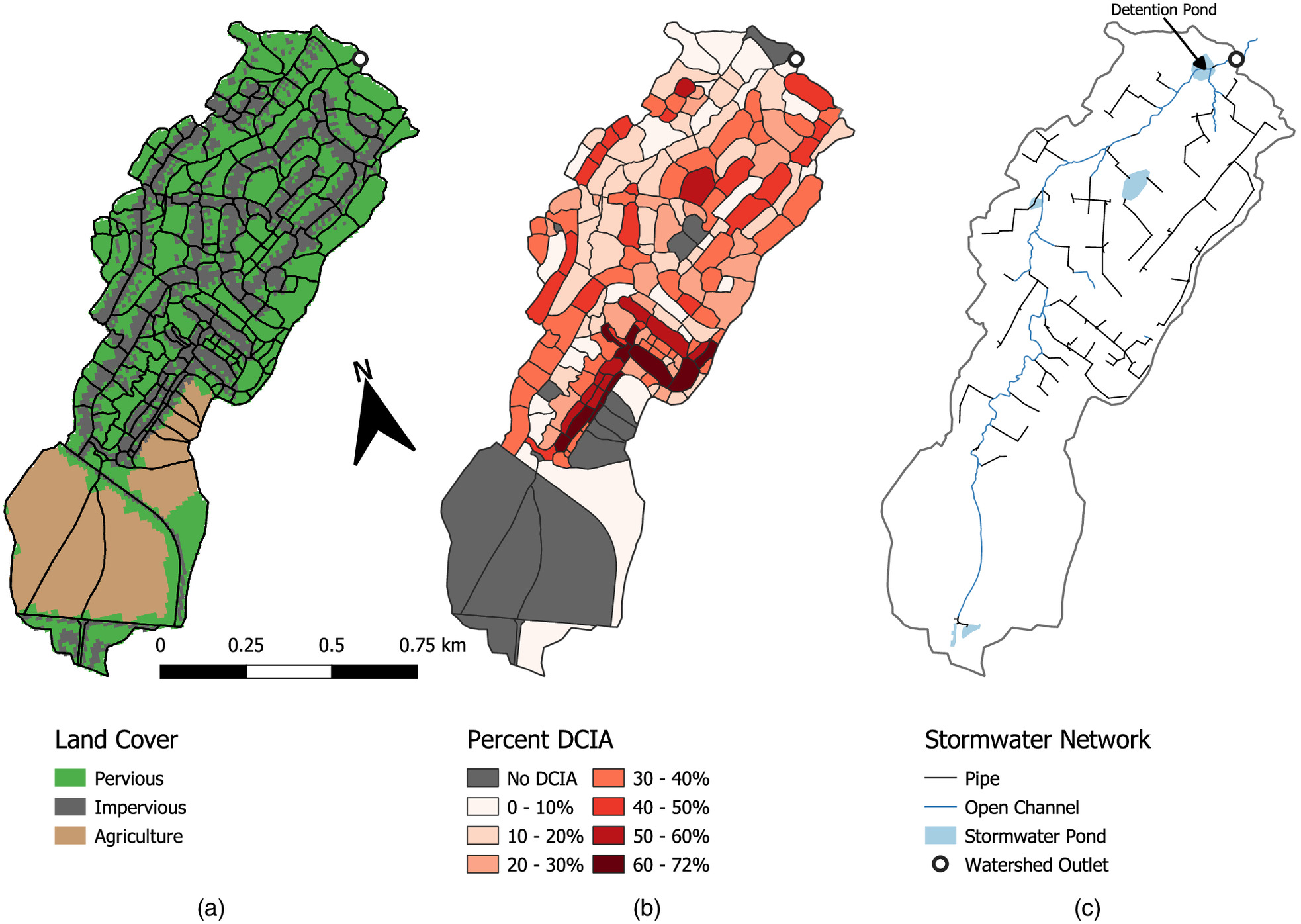
We modeled GSI performance in each of the representative cities identified above using the EPA Storm Water Management Model (SWMM) Version 5.1.013 (Rossman 2015). To isolate the effects of climate and GSI design alone (as opposed to watershed characteristics), we used the same modeled watershed fed with different climate data. We used a SWMM model developed for Shayler Crossing, a

{\sim 0.92 - km}^{2}

watershed east of Cincinnati, Ohio (Fig. 1) (Lee et al. 2018). At the time the model was developed, the watershed was 62.6% urban, 25.6% agriculture, and 11.8% forested, with low-infiltration soils (Lee et al. 2018). Total imperviousness and directly connected imperviousness were respectively 23.6% and 18.5% of the watershed area. Lee et al. developed this SWMM model with a unique approach to account for both indirectly connected and directly connected impervious area to more realistically simulate stormwater runoff. We used their calibrated model with some minor modifications to reduce water balance errors and allow continuous simulations (see the Supplemental Materials for details). Model performance was essentially unchanged after these modifications [Nash-Sutcliffe

coefficient = 0.853

,

R^{2} = 0.861

, compared with 0.852 and 0.871, respectively, from Lee et al. (2018); see Fig. S3]. The model underpredicted total runoff volume by 11.6%.

Fig. 1. Shayler Crossing watershed showing: (a) subbasins with land cover; (b) directly connected impervious area percentage; and (c) existing stormwater network, including pipes, open channels, and stormwater ponds. Watershed-scale metrics calculated using inflows to in-line detention pond near watershed outlet. [Land cover map reprinted from Hoghooghi et al. (2018) under Attribution 4.0 International (CC BY 4.0) license (https://creativecommons.org/licenses/by/4.0/).]

We used this SWMM model to compare current conditions (baseline) to various GSI scenarios using rainfall data from each of the nine cities identified in the rainfall region analysis. Only precipitation and temperature data varied between cities, meaning that we only analyzed climate effects and no other region-specific variables (e.g., in situ soil type). We conducted two sets of analyses: design storm–based modeling and continuous simulations (see the relevant sections for more details).

The baseline scenario corresponds to current watershed conditions (land use and stormwater network, including five stormwater ponds). The Lee et al. model subdivides each subbasin into several areas. An indirectly connected impervious area (ICIA) drains into a buffering pervious area (BPA) before draining to the subbasin outlet. A standalone pervious area (SPA) and a directly connected impervious area (DCIA) both drain directly into the outlet (Fig. S4). Lee et al. manually delineated each subbasin into these different areas based on satellite imagery. For example, major buildings were included as DCIAs because downspouts are plumbed directly into the stormwater system. Roads with curb-and-gutter drainage systems, and other impervious areas connected to these roads, were also classified as DCIAs. More details on this subbasin categorization can be found in Lee et al. (2018). For the different GSI scenarios, we simulated a single bioretention cell per subbasin to capture runoff from the DCIA. The area of the SPA was reduced based on the size of the bioretention cell (Fig. S4).

Each bioretention cell had the same basic design: 7.6 cm (3 in.) ponding depth, 45.7 cm (18 in.) soil depth, and 30.5 cm (12 in.) storage zone depth, with an upturned elbow underdrain (see Table S2 for details). This basic design was meant to be representative of a typical bioretention cell (e.g., Lewellyn and Wadzuk 2019). While results would likely be different for other designs, we expect the general trends to be consistent. Different scenarios were run with varying bioretention soil types and cell sizes. Three soil types were selected to represent high (loamy sand), medium (loam), and low (clay loam) infiltration capacity. We chose these soil types to compare performance across a range of infiltration capacities (hydraulic conductivity varies by

30 \times

between the selected soils). While the latter two soils have infiltration rates lower than typically required in design manuals, results from these soil types can help assess how soil clogging with fine sediment may affect performance (e.g., Davis et al. 2009). Bioretention size was based on a drainage area ratio [Eq. (1)]:

DAR = \frac{Area of bioretention}{Area of DCIA} \times 100 %

(1)

For this analysis, we used DARs of 1%, 5%, 10%, 15%, and 20%. Since only the surface area of the bioretention area changed, each of these DARs has an inherent maximum water storage capacity (which also changes based on soil type). For example, for a high-infiltration soil, each DAR has a total storage capacity of

0.39 - 7.72 cm

(

0.15 - 3.04 in.

) of surface runoff from its contributing watershed (see Table S2). Design manuals vary in their DAR recommendations, ranging from 3% to 43% (Stander et al. 2010). The literature has similar variability in DARs analyzed. For studies that reported this metric, values ranged from 1% to 25% (Boancă et al. 2018; Li et al. 2009; Stander et al. 2010; Wright et al. 2018). More commonly, design standards are based on depths of runoff that should be captured and/or treated by a stormwater control measure (McPhillips et al. 2020).

Design Storm Analysis

For the initial analysis, we modeled GSI performance for design storms of various sizes (1-month through 100-year). Designs storms represent storm depths and durations with various probabilities of occurring (usually expressed as a return period) and are commonly used to size stormwater facilities (ASCE EWRI/WEF 2012; McPhillips et al. 2020). We use them in this analysis because of their design relevance and to facilitate comparisons between storms of similar frequency in different climates. We used the NOAA Atlas 14 database (NOAA National Weather Service 2017) to obtain 24-h design storm depths for each city for 2-, 10-, 50-, and 100-year storm events. The exception was Seattle, Washington, which was not incorporated into Atlas 14. We used design storm depths from the Seattle stormwater manual, Protecting Seattle’s Waterways (City of Seattle 2016). Since rainfall depths for storms smaller than a 1-year event were not available, we estimated depths of 1-month and 6-month storms as one quarter and one half of a 2-year event, respectively. We used the Soil Conservation Service (SCS) design storm method to convert these storm depths into 24-h rainfall hyetographs (USDA 1986). We used the appropriate region-specific SCS design hyetographs for each city: Type I for Los Angeles, Type IA for Seattle, Type III for New Orleans, and Type II for the remaining cities. Some municipalities may have developed more locally appropriate design storms (Los Angeles, for example); however, we chose SCS design storms because of their widespread use.

For each city, we ran SWMM 90 times for each combination of 6 storm events (1- and 6-month and 2-, 10-, 50-, and 100-year), 5 drainage area ratios (1%, 5%, 10%, 15%, and 20%), and 3 bioretention soil types (high, medium, and low infiltration) plus an additional 6 simulations with no bioretention areas (baseline for each storm event). We simulated 48 h for each storm event (24-h storm plus an additional 24 h). We quantified bioretention performance in several ways. We estimated percentage reduction in peak flow rate and total runoff volume for the watershed using Eq. (2)

% r e d = \frac{X_{b a s e l i n e} - X_{G S I}}{X_{b a s e l i n e}} \times 100 %

(2)

where

X_{baseline}

= peak flow rate (or runoff volume) for the baseline scenario; and

X_{GSI}

= peak flow rate (or runoff volume) for a scenario with green stormwater infrastructure. Watershed-scale metrics were calculated using inflows to the in-line detention pond near the watershed outlet to remove the effects of this structure on reducing peak flows. Furthermore, we compared subbasin-scale performance with watershed-scale performance. We calculated percentage reduction in peak flow rate and runoff volume for each subbasin and calculated a weighted average for the watershed based on subbasin areas. We compared this value with what was calculated at the watershed outlet. Comparing these values provided an estimate of the differences between GSI performance at the subbasin/local scale versus the watershed scale.

Continuous Simulations

While analyses based on design storms are useful, they cannot fully represent conditions experienced by stormwater infrastructure in the real world (Voter and Loheide 2021). Continuous simulations of multiple years of rainfall in various climates provide a more realistic assessment of GSI performance. Importantly, this accounts for the effects of antecedent conditions and storm sequence that the design storm approach misses. We performed three years of continuous simulations for each city for a single GSI scenario (drainage area ratio of 10%). We obtained hourly precipitation and daily temperature and wind data for NOAA National Climate Data Center (NCDC) stations in each of the nine cities selected as part of the precipitation region analysis. For each city, we collected hourly precipitation data for all calendar years from 1981 to 2010, omitting any years with more than 5% missing data. We then selected a representative “normal,” “dry,” and “wet” year based on total annual precipitation amounts. “Normal” years were near the median of this period of record, while “dry” and “wet” years were near the 10th and 90th percentiles, respectively. Each of these three years was simulated separately (i.e., three 1-year simulations).

We computed several metrics to assess bioretention performance for each scenario. We quantified reductions in peak flow and runoff volume for each storm event in the continuous simulations. Events were defined as at least 0.25 mm (

0.01 in.

) of precipitation preceded by at least 6 h of no rainfall. At the annual scale, we computed high pulse count (HPC) and high pulse duration (HPD; number of times and total duration above some flow threshold) based on modeled in-stream discharge (DeGasperi et al. 2009; Wright et al. 2018). These physically-based metrics are negatively correlated with stream biotic indices (i.e., lower HPC and HPD means better stream health) and were chosen because they quantify the ability of GSI to change watershed hydrology in a way that provides meaningful in-stream benefits. The flow threshold was set as

2 \times

the mean flow for the baseline scenarios (DeGasperi et al. 2009). We also quantified the reduction in annual surface runoff from the entire watershed and changes in the Richards-Baker flashiness index (Baker et al. 2004). These watershed-scale metrics were calculated using inflows to the in-line detention pond near the watershed outlet.

Furthermore, we examined the performance of individual bioretention areas to determine when and why there was outflow. Specifically, we quantified the amount of outflow caused by infiltration excess (i.e., the intensity of inflow was higher than the infiltration capacity of the bioretention soil) and saturation excess (i.e., back-to-back events, which did not allow the bioretention area to drain sufficiently before additional inflow). Saturation excess was defined as the bioretention soil being

> 90 %

saturated at the beginning of a storm event. All streamflow metrics were calculated using runoff data with a 15-min time step. All outflow data for individual bioretention areas had a 1-min time step.

We used R Version 3.6.0 (R Core Team 2021) to run SWMM and perform all analysis. We used the following packages: cluster (Maechler et al. 2019), dplyr (Wickham et al. 2021), insol (Corripio 2019), lubridate (Grolemund and Wickham 2011), prism (Hart and Bell 2015), raster (Hijmans 2019), RColorBrewer (Neuwirth 2014), rnoaa (Chamberlain 2019), sf (Pebesma 2018), stringr (Wickham 2019), swmmr (Leutnant et al. 2019), vioplot (Adler and Kelly 2019), viridis (Garnier et al. 2021), and zoo (Zeileis and Grothendieck 2005).

Results

US Precipitation Regions

We created 10 unique precipitation regions for the conterminous US (Fig. 2, Table 1). The clustering analysis initially created 8 regions, but we subdivided Regions 2 and 3 because they had geographically distinct areas that, upon more detailed analysis, displayed some unique precipitation patterns (see the Supplemental Materials). Delineations between regions are not exact, but instead show general geographic trends in precipitation patterns that may affect the performance of all stormwater infrastructure, including GSI. These regions follow recognizable climate trends and bear some resemblance to other climate classifications. For example, the Gulf region stands out from the rest of the southeast, largely due to its higher total rainfall and storm intensity. The gradient between the arid west and humid east is also clearly delineated (border between Regions 8 and 3, near the 100th meridian). The desert southwest (including southern California and the Central Valley) is unique due to its high rainfall seasonality and long interstorm durations. The effects of mountains in the West (and to a smaller extent the Appalachians in the East) can also be identified. Mountains have higher precipitation with higher proportion of snowfall than their surrounding lowlands, giving these areas more variable regional classifications, especially where there are large elevation gradients (e.g., Rocky Mountains and Sierra Nevada). Representative cities were selected for each region except Region 6 (western mountains) because of its lack of large cities and long-term weather data in this region (Fig. 2, Table 1).

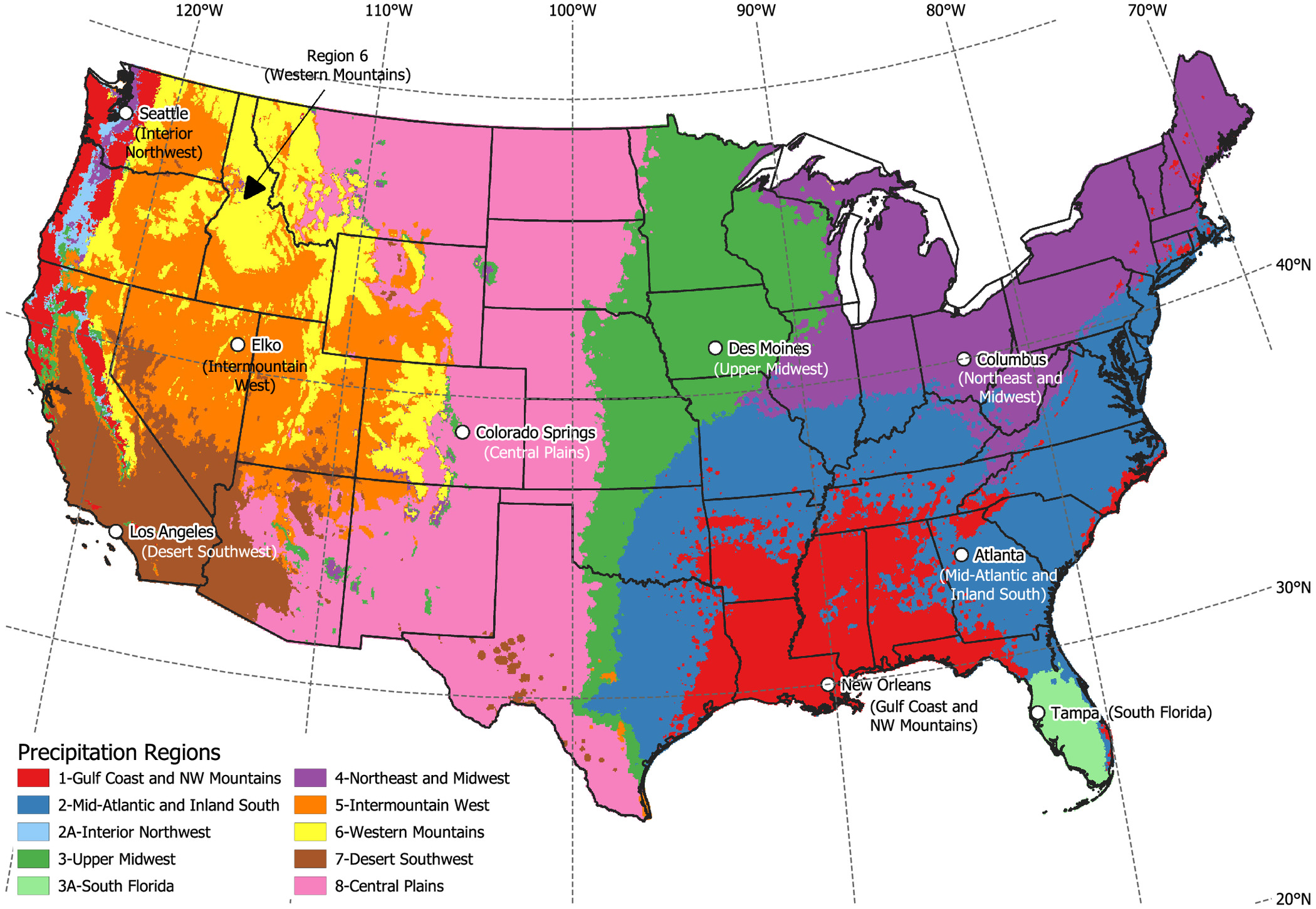
Fig. 2. Precipitation regions for the conterminous US, including the representative city for all but Region 6.

Table 1. Description of precipitation regions, including the representative city and the climate station where precipitation, temperature, and wind speed data were collected for continuous simulations

Region number	Name	Description	Representative city	NOAA NCDC climate station
1	Gulf Coast and Northwest Mountains	Wet, with frequent precipitation, frequent high-intensity events, and mixed seasonality and snowfall (high in Northwest, low in Gulf)	New Orleans	COOP: 166660 New Orleans Airport
2	Mid-Atlantic and Inland South	Moderate to wet, with frequent precipitation, low snowfall, frequent high-intensity events, low seasonality	Atlanta	COOP:090451 Atlanta Airport
2A	Interior Northwest	Moderate to wet, with frequent precipitation, low snowfall, frequent high-intensity events, high seasonality	Seattle	COOP:457473 Seattle-Tacoma Airport
3	Upper Midwest	Moderately wet, moderate snowfall, moderate seasonality, highsummer rainfall with moderate intensity	Des Moines, Iowa	COOP:132203 Des-Moines Airport
3A	South Florida	Wet, no snowfall, moderate seasonality, high summer rainfall with moderate intensity	Tampa, Florida	CCOP:088788
3A	South Florida		Tampa, Florida	Tampa Airport
4	Northeast and Midwest	Moderate to wet, frequent precipitation, moderate snowfall, low seasonality, moderate intensity	Columbus, Ohio	COOP:331786 Columbus Airport
5	Intermountain West	Arid, moderate snowfall, moderate seasonality, low-intensity events, moderate interstorm duration	Elko, Nevada	COOP:262573 Elko County
6	Western Mountains	Moderately wet, frequent precipitation, high snowfall, moderate seasonality, few high-intensity events	—	—
7	Desert Southwest	Arid, infrequent precipitation, low snowfall, high seasonality, low summer rainfall, few intense events, high interstorm duration	Los Angeles	COOP:045114 Los Angeles Airport
8	Central Plains	Arid, relatively infrequent precipitation, low-moderate snowfall, high seasonality and summer rainfall, moderate intensity	Colorado Springs, Colorado	COOP:051778 Colorado Springs Airport

Design Storm Modeling

Design storm simulations show three trends in GSI effectiveness: (1) increasing effectiveness with larger bioretention areas (higher DAR), (2) decreasing effectiveness with lower soil infiltration capacity, and (3) decreasing effectiveness with larger storm events (Fig. 3). For a given storm size and soil infiltration capacity, a larger bioretention area yields greater reductions in runoff volume and peak flows. Runoff volume reduction increases linearly with DAR [Figs. 3(j–l)]. The exception is for some small storm events (

< 5 cm / 2 in.

), where a larger bioretention area does not improve performance because all available runoff has already been captured. Peak flow reduction shows a much stronger threshold effect with increasing DAR [Figs. 3(d–f)]. For many storm events, there is little or no peak flow reduction until the bioretention cell becomes sufficiently large.

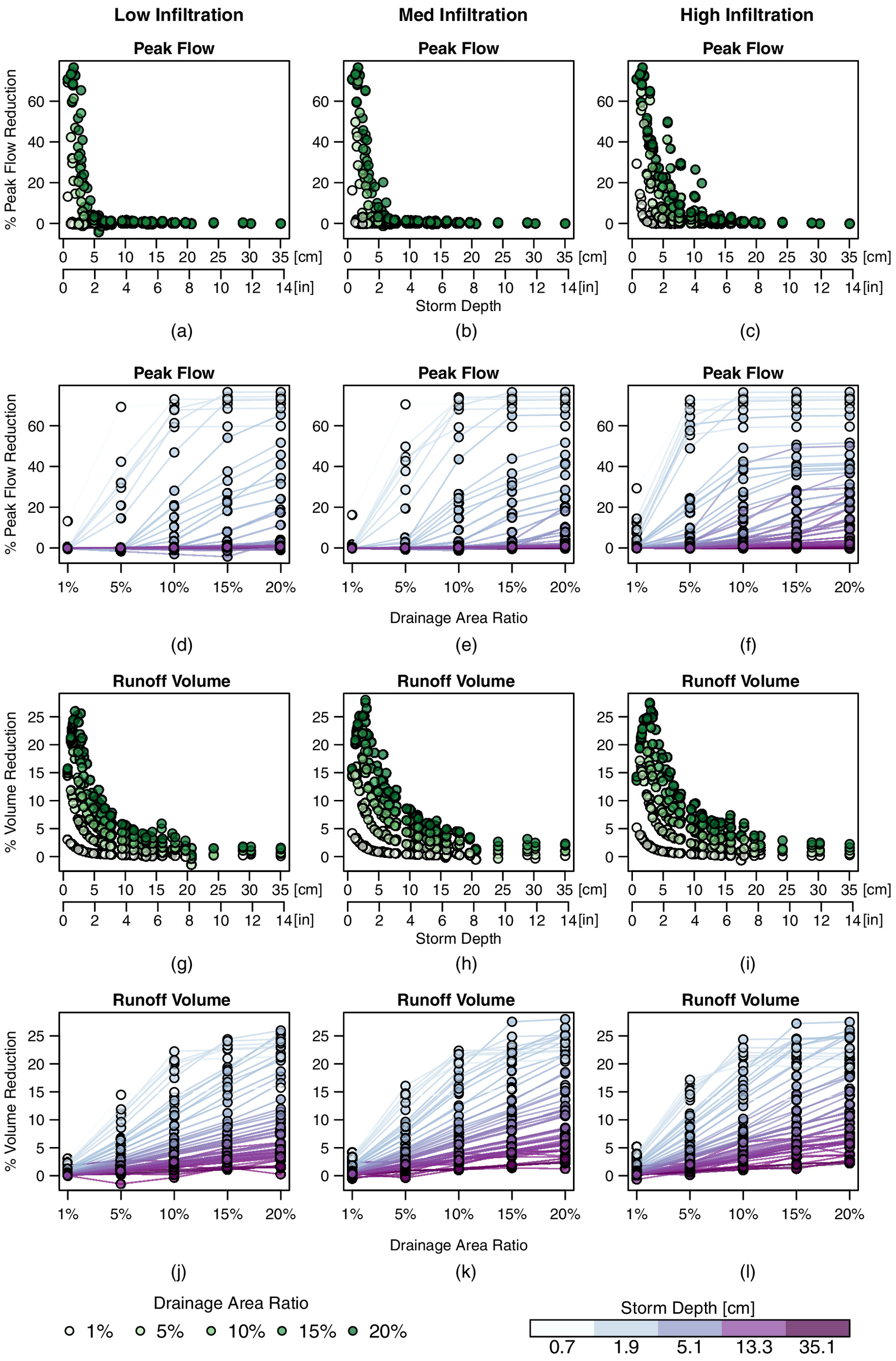
Fig. 3. Reduction in peak flow rate and total runoff volume measured at watershed outlet for all design storm scenarios: (a–c and g–i) performance versus storm with depth points colored by DAR; and (d–f and j–l) performance versus DAR with points colored by storm depth.

The infiltration capacity of the bioretention soil has a larger effect on peak flow reduction than on runoff volume reduction [Figs. 3(a–c and g–i)]. Notably, there is little to no peak flow reduction above

\sim 5 cm

(

2 in.

) of rainfall for low-infiltration soils, but there is appreciable peak flow reduction up to a

10 - cm

(

4 - in.

) storm for high-infiltration soils. This suggests that the infiltration rate can significantly affect peak flow reduction but has less effect on the total volume of runoff that is eventually retained.

Storm event size has the largest effect on the performance of GSI. Unsurprisingly, there is less peak flow and runoff volume reduction as storms get bigger. However, for large enough bioretention cells, there can still be a 3%–10% runoff volume reduction for storms larger than 10 cm (

4 in.

). There is essentially no peak flow reduction for these large storms, especially for low- and medium-infiltration soils. Fig. 3 lumps results for all cities together, but there is significant variability among them (see the Supplemental Materials for full results). Since storm depth for a given recurrence interval can differ significantly, so does GSI performance. For example, GSI may provide significant peak flow and volume reduction for a 100-event in Elko, Nevada (storm depth

6.7 cm / 2.64 in.

) but have essentially no effect on the runoff hydrographs for a 100-year event in New Orleans, Louisiana (

35 cm / 13.8 in.

). The shape of the storm hyetograph may also affect GSI performance, at least for peak flow reduction. For example, a storm in Seattle, Washington (early rainfall peak with long tail) showed greater peak flow reduction than a similarly sized storm in Tampa, Florida [peak in middle of storm, more equally weighted rainfall through time; see Figs. S14(c) and S20(b)]. Peak flows were also

\sim 5

times higher in Tampa than in Seattle for this similar rainfall depth, solely due to changes in the distribution of the rainfall through time.

Peak flow reduction is greater at the watershed-scale than the subbasin scale (Fig. 4). In most cases, peak flow reduction in individual subbasins is small. However, bioretention areas do significantly reduce runoff volume on the rising and falling limbs of the hydrograph. This has a cumulative effect at the watershed scale of reducing peak flow rates. While this may cause subbasin runoff hydrographs to be slightly flashier with GSI, the net effect at the watershed scale is reduced flashiness, as discussed later.

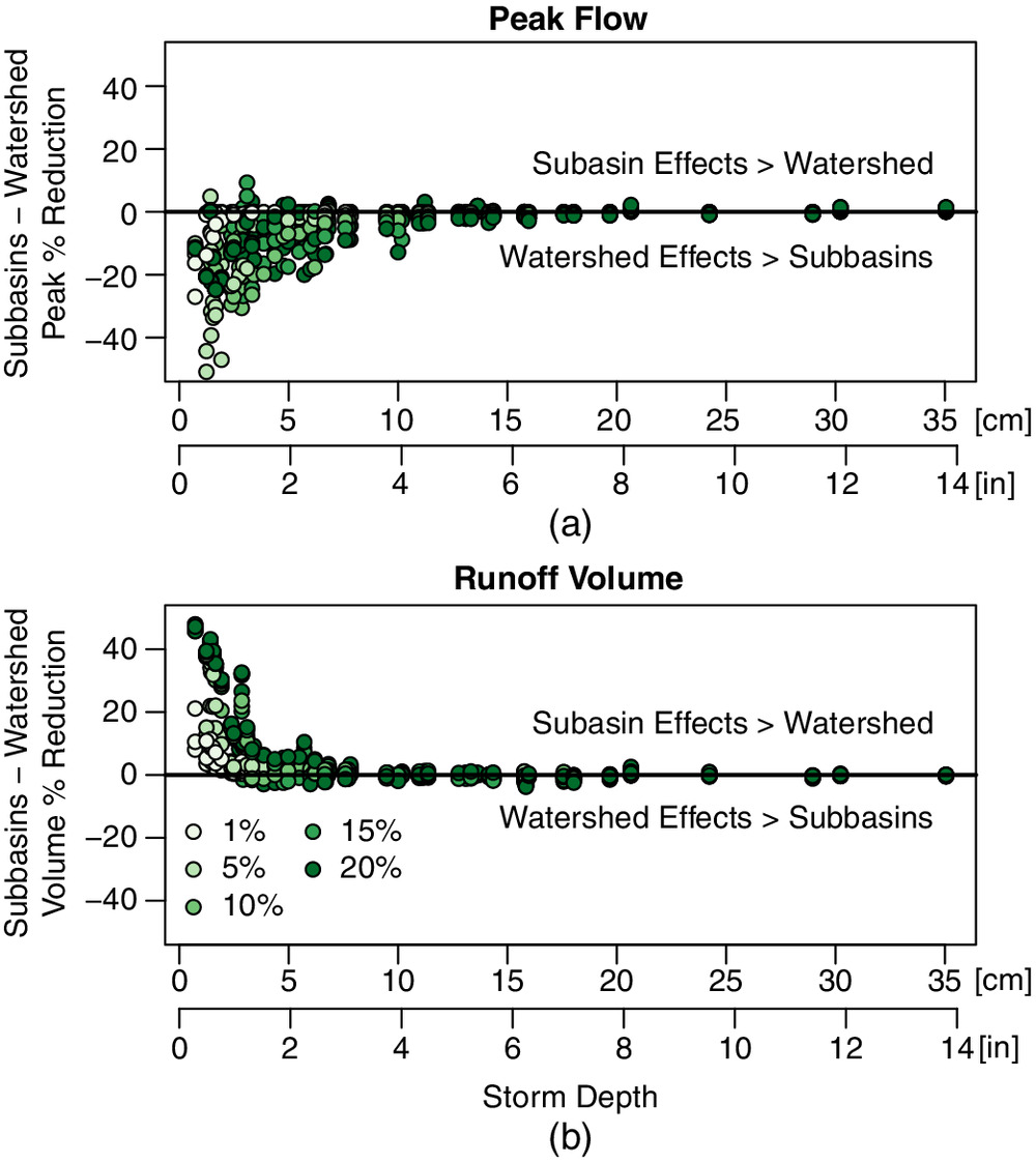
Fig. 4. Difference between subbasin-scale and watershed-scale effects of GSI for design storm simulations for (a) peak flow reduction; and (b) runoff volume reduction (points colored by DAR).

Runoff volume reduction shows the opposite trends: benefits are greater at the subbasin scale than the watershed scale (Fig. 4). This is primarily because the bioretention areas are increasing subsurface flow to the stream, leading to a gentler receding limb of the hydrograph and increasing stream base flow (see continuous simulation results below). Since we measure only surface runoff from the subbasins, this gives greater runoff reduction benefits at this scale. Fig. 4 also shows that performance at the subbasin and watershed scale is similar above

\sim 10 cm

(

4 in.

) for peak flows and

\sim 7.5 cm

(

3 in.

) for runoff volume. However, this does not mean that there is no reduction in these flow metrics above these thresholds (Fig. 3); it only means that those reductions are the same at the subbasin and watershed scales.

Continuous Simulations

Continuous simulations for the nine cities (for DAR of 10% only) show similar reductions in peak flows and surface runoff as event-scale results (Fig. 5). High pulse counts (HPCs) are reduced between 20% and 75%. Generally, HPC reduction is greatest for higher-infiltration soils in cities with lower annual precipitation. High pulse duration (HPD) sometimes increases and sometimes decreases with the addition of GSI. Higher subsurface flows to the stream (from infiltrating runoff in the bioretention areas) extend the recession limb of storm hydrographs, increasing HPD in some cases. HPD is also very sensitive to the flow threshold used. We used twice the mean flow (after DeGasperi et al. 2009), but this is not necessarily a geomorphically or biologically relevant flow value.

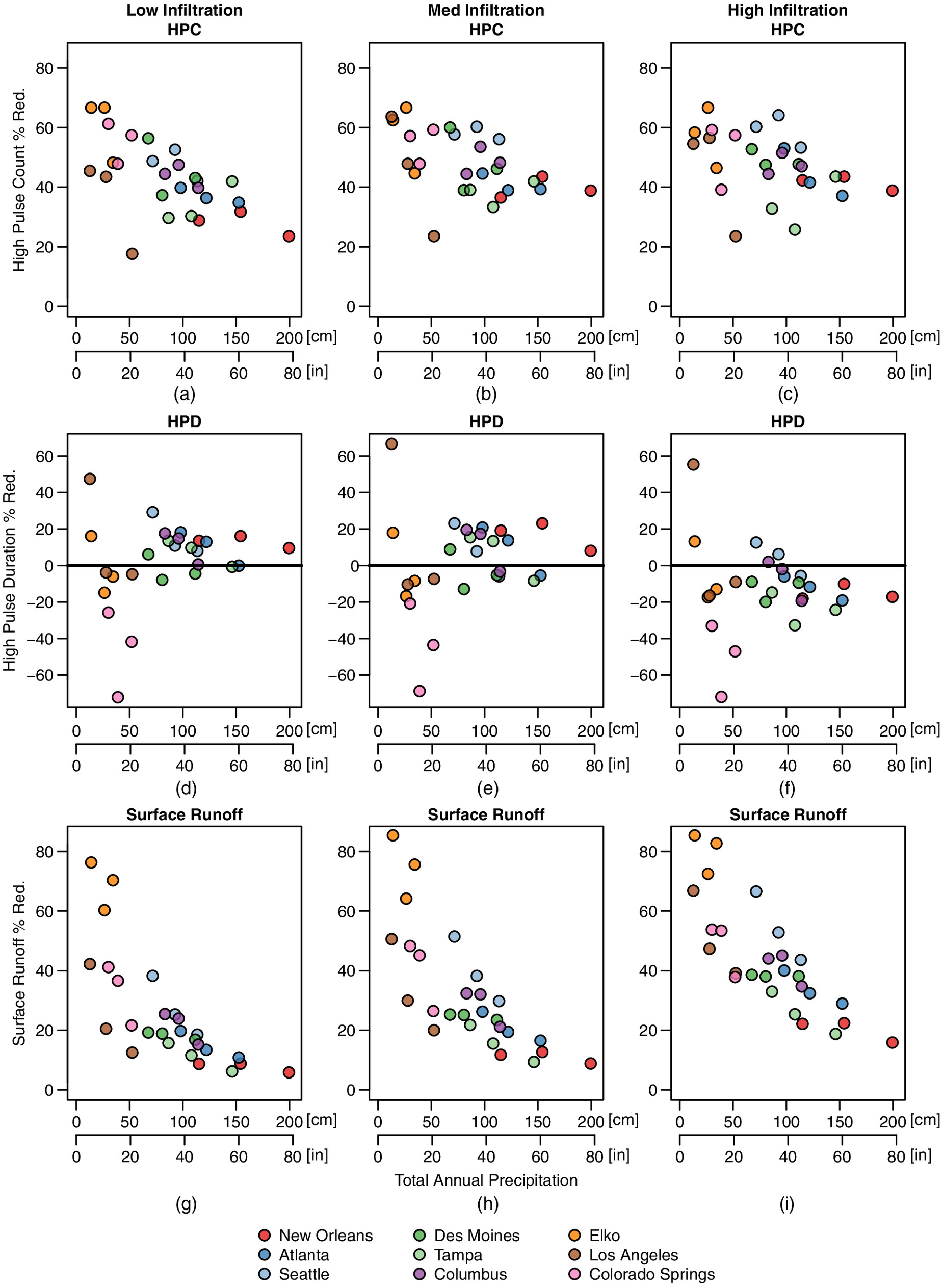
Surface runoff shows a much more predictable response, with greater reductions at higher soil infiltration rates. Surface runoff also shows the strongest relationship with total annual precipitation, with wetter cities (e.g., New Orleans) showing less runoff reduction than more arid cities (e.g., Elko). Despite the reduction in surface runoff, total water export from the basin actually increased in all cases with GSI. Again, this was in response to higher subsurface flow, which significantly increased base flow and therefore total annual flow. Stream flashiness also decreased in every case when GSI was added (median 19% reduction, ranging 7%–46%; Figs. S43–S51), suggesting that bioretention areas help reduce rapid changes in discharge in the receiving streams. The reduction in flashiness was greater for higher-infiltration soils and years with less rainfall.

Even with a DAR of 10%, not all runoff events are fully captured by the bioretention areas. Total outflow ranged

\sim 10 % - 80 %

of total bioretention inflow for all cities and years modeled [Figs. 6(a–c)]. Outflow events primarily occurred (by either surface overflow or drain outflow) from high-intensity events (i.e., the rate of inflow exceeds the infiltration rate of the soil) or from back-to-back events (i.e., the bioretention area was still saturated from a prior storm event). More outflow came from high-intensity events than back-to-back events [Figs. 6(d–i)]. Outflow from high-intensity events was strongly dependent on soil type, with higher infiltration soils better able to capture intense runoff. These soils also had slightly less outflow from back-to-back events. However, total outflow changed very little as soil infiltration capacity increased—even if surface overflow decreased, drain outflow increased. This suggests that while bioretention soil infiltration capacity controls the type of outflow (i.e., surface or drain), the total volume captured changes very little.

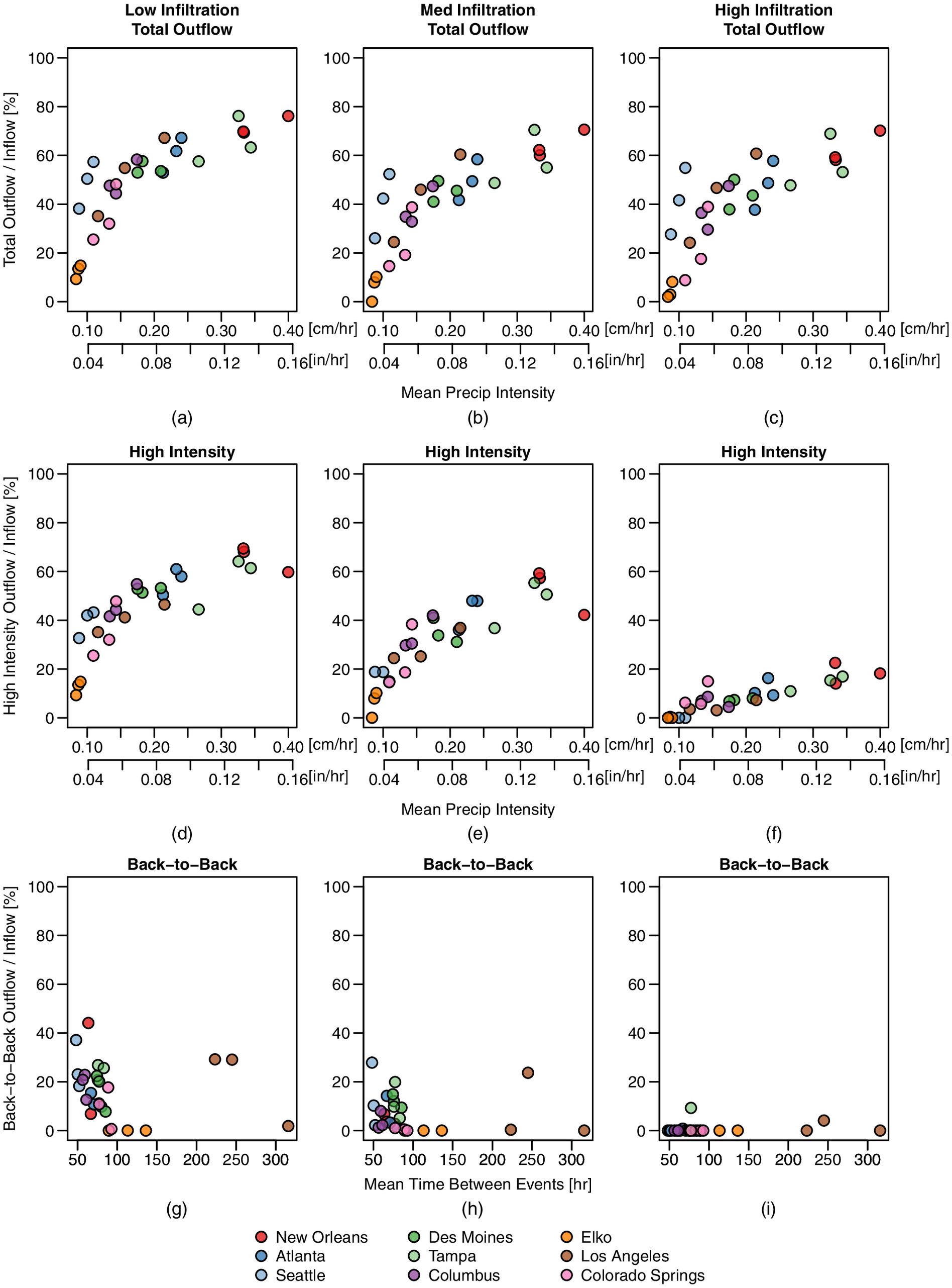
Fig. 6. (a–c) Total outflow from bioretention cells; (d–f) outflow from high-intensity storms; and (g–i) outflow from back-to-back events—all as percent of inflow for each of three years modeled for each city. All data are for 10% DAR. Note some double counting of outflow because an event can be classified as high-intensity and “back-to-back”.

Rainfall patterns can also have a significant effect on overflow from bioretention areas. Bioretention areas overflowed more in cities with frequent, high-intensity storms than in locations with infrequent lower-intensity, rainfall (Fig. 6). For high-infiltration soils, outflow from high-intensity events increases as mean precipitation intensity increases. Similarly, outflow from back-to-back events increases as interstorm duration decreases [with the exception of high-infiltration soils, which eliminate nearly all outflow from back-to-back events; Fig. 6(j)]. Seasonality also plays a role. For example, in Colorado Springs GSI outflow occurs primarily in the summer when high-intensity thunderstorms are common (Fig. S60). In Columbus, on the other hand, GSI outflow occurs consistently throughout the year, as does rainfall (Fig. S57).

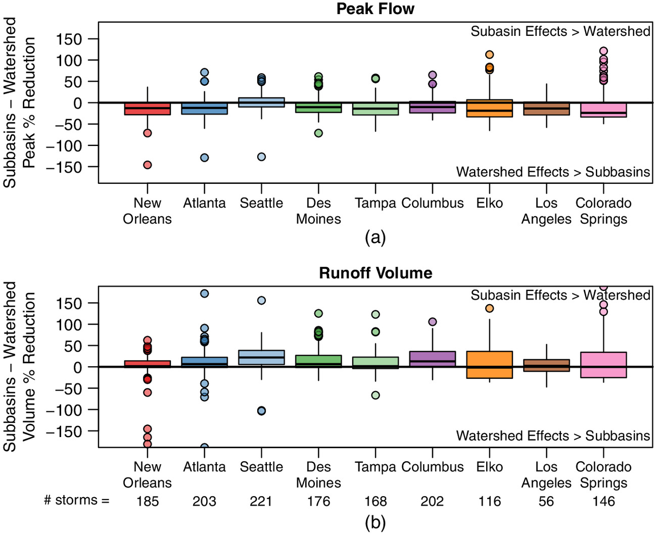
Differences between subbasin-scale and watershed-scale benefits were generally similar to the design storm analysis (Fig. 7). Watershed-scale reductions in peak flows were generally larger than what was observed at the subbasin scale. Volume reductions at the watershed scale generally were smaller than what was observed at the subbasin scale. However, for both peak flow and runoff volume, there were events where opposite trends were observed. There were slight variations by city, but interevent differences (variation within boxplots) appear to be larger than differences between cities/climates (variations between boxplots).

Fig. 7. Difference between GSI subbasin-scale and watershed-scale effects for continuous simulations for (a) peak flow reduction; and (b) runoff volume reduction by city. Boxplots show distributions of differences by event for all three years of analysis (dry, normal, wet); $y$ -axis scales cropped for readability, excluding some outliers. Data shown only for high-infiltration bioretention soils to avoid double-counting rainfall events.

Discussion

We modeled the effectiveness of different GSI scenarios at reducing runoff volume and peak flow rates in a small watershed under different rainfall regimes. Hydrologic benefits of GSI can be significant, especially for smaller rainfall events, but they are strongly dependent on design and climate.

Local-Scale and Watershed-Scale Effects Are Significantly Different

Watershed-scale benefits of GSI are not the same as what is observed at the site scale (Jefferson et al. 2017). Subbasin- or site-scale benefits of bioretention areas (Jennings 2016; Wadzuk et al. 2017; Winston et al. 2016) are generally reported to be significantly greater than watershed-scale benefits (Hoghooghi et al. 2018; Hopkins et al. 2019; Woznicki et al. 2018). We found this to be true for runoff volume reduction; however, we found the opposite results for peak flow reduction (Figs. 4 and 7).

For volume reduction, watershed-scale benefits never exceed subbasin-scale benefits in design storm modeling (Fig. 4) and they do so only rarely in the continuous simulations (Fig. 7). As noted above, this was partially due to measuring surface runoff from subbasins but cumulative streamflow volume in watersheds. The addition of GSI increased infiltration and base flow reaching the stream, which was counted as watershed-scale runoff. The modeled watershed-scale water balance supports this, showing an increase in the proportion of subsurface water reaching stream channels for all cities with the addition of GSI (Fig. S6). However, our groundwater model was parametrized to represent conditions in the study watershed, and was kept constant for simulations in all cities. Groundwater dynamics vary with climate and geology, and a different model parameterization (or a more sophisticated groundwater model) would potentially yield different results. Increased groundwater inputs to the stream are generally considered beneficial, especially in urban areas where natural base flow regimes have been altered (Bhaskar et al. 2016). Therefore, the smaller runoff reduction benefits we observed at the watershed scale are not necessarily detrimental. Still, it may be unreasonable to expect the benefits of an individual bioretention area to directly translate to watershed-scale reductions in runoff volume.

On the other hand, watershed-scale peak flow reductions are often greater than reductions at the subbasin scale (Figs. 4 and 7). Both the magnitude and timing of subbasin peak flows showed little or no change after GSI installation. What did change, however, was the shape of the runoff hydrograph. The bioretention cells captured runoff and “shaved” flow off the rising and falling limbs of the hydrographs, reducing runoff duration. As these altered hydrographs were routed downstream and combined with those from other subbasins, the cumulative effect on peak flows at the watershed outlet was much greater than what was observed in any individual subbasin. This result may be specific to the study watershed—watersheds with different shapes, topographies, drainage systems, and other characteristics will have unique hydrograph-routing characteristics.

Others have noted the potential for stormwater infrastructure to increase watershed peak flows by “stacking” or syncing peaks from different subbasins (Emerson et al. 2005; McCuen 1979). However, we have demonstrated that the opposite effect is also possible when using infiltration-based stormwater controls. This points to a potential management approach for strategically designing individual stormwater infrastructure to yield greater cumulative watershed-scale benefits than could otherwise be achieved (McCuen 1974).

Bioretention Size and Climate Affect Performance More Than Soil Infiltration Rate

Bioretention design (DAR and soil infiltration rate), storm event size, and climate all interact to affect the ability of green infrastructure to mitigate watershed-scale hydrologic effects of urbanization. Bioretention performance improves as bioretention cells get larger (Boancă et al. 2018; Tirpak et al. 2021; Wright et al. 2018) or more of the watershed is treated with GSI (Bell et al. 2020). However, the relationships between bioretention size and different performance metrics are not consistent. For example, we found generally linear increases in runoff volume reduction with increasing DAR [Figs. 3(j–l)], similar to those in Boancă et al. (2018). On the other hand, we found a nonlinear relationship between DAR and peak flow reduction [Figs. 3(d–f)], similar to that in Wright et al. (2018), who showed little improvement in peak flow metrics above a certain threshold bioretention size. These linear relationships with runoff volume and nonlinear relationships with peak flow also hold as more of the watershed is treated with GSI (Bell et al. 2020). These results suggest that there may be an upper limit to peak flow reduction as bioretention cells get bigger but that they continue to reduce runoff volume. There also appears to be a smaller potential to reduce peak flows than to reduce runoff volume, at least for larger storm events (Fig. S5). The primary design goal of bioretention is usually to target runoff volumes rather than peak flows (McPhillips et al. 2020). This helps explain why these infiltration-based practices yield bigger benefits for runoff reduction than peak flow, as opposed to detention-based stormwater controls that are designed for peak flow reduction (Bell et al. 2020).

The benefits of green stormwater infrastructure tend to decrease with increasing storm event depth (Fry and Maxwell 2017; Giese et al. 2019; Hopkins et al. 2019; Hu et al. 2019; Palla and Gnecco 2015; Woznicki et al. 2018). This is unsurprising since many bioretention areas are designed to capture runoff from smaller, more frequent storms (McPhillips et al. 2020). Still, we showed that, for storm events

> 10 - 13 cm

(

4 - 5 in.

), there may a 5%–10% reduction in watershed runoff volume, even if there is very little benefit for peak flows. This is a larger storm depth than even the 20% DAR bioretention area is sized to capture (

\sim 7.7 cm / 3 in.

), indicating that fully functioning bioretention areas can provide volume reduction benefits beyond their design capacities. Similar results have been reported by others. A monitoring study in the mid-Atlantic found that during a large storm (Tropical Storm Irene, a “1,000-year” rainfall event), runoff volume was smaller from a watershed with distributed GSI than from a watershed with conventional stormwater infrastructure, although peak flow rates were similar (Loperfido et al. 2014). However, small GSI may be ineffective during large storm events that contribute significantly to annual runoff volumes and may need to be paired with larger infrastructure (Woznicki et al. 2018). Other modeling studies have found measurable reduction in peak flow even during large storm events (Fry and Maxwell 2017; Hu et al. 2019); however, these studies simulated a high-density GSI and their 100-year storms were smaller (

\sim 7.6

and

14 cm / \sim 3.0

and

5.5 in.

, respectively) than many of the 100-year storm events we analyzed.

Climate effects on bioretention performance extend beyond just the total rainfall depth of an individual storm event. The continuous simulation results showed that watershed-scale (Fig. 5) and site-scale (Fig. 6) GSI performance were related to multiple precipitation metrics (e.g., total annual precipitation, mean storm intensity, mean interstorm duration). Rainfall seasonality (see the Supplemental Materials) is also important and can affect the timing and amount of outflow from bioretention areas. This is important because both the amount and timing of runoff affect water quality and ecological impacts on receiving streams [e.g., winter runoff, which can carry dangerously high concentrations of salt (Tiwari and Rachlin 2018)]. The effects of multiple precipitation metrics on GSI performance can also be seen by comparing differences between wet, normal, and dry years for individual cities. In New Orleans, for example (red points in Fig. 5), there is little variability in performance between years, despite a large range in annual rainfall. Seattle (light blue) and Los Angeles (brown) show much greater variability in GSI performance. This suggests that selecting different “representative” years yields very different predictions of GSI efficacy, at least in some climates.

Most other studies on climate effects on GSI performance also analyzed within-storm climate metrics (e.g., rainfall depth, intensity, duration) (Sohn et al. 2019). Voter and Loheide (2021), however, found that other climate metrics [such as ratio of potential evapotranspiration (PET) and precipitation (P), fraction of time raining, and temporal correlations between PET and P] are more important predictors of GSI performance over multiple years. For our continuous simulations, high pulse count and runoff volume reductions were negatively correlated with total annual rainfall, the difference in P and PET, and rainfall intensity metrics. However, all these metrics had strong, significant positive correlations with total annual rainfall, making it unclear what the specific physical driver is in GSI performance.

Storm intensity and interstorm duration were both correlated with outflow from individual bioretention cells. High-intensity events, rather than frequent storms, are responsible for most of the outflow (Fig. 6). Many researchers have noted that rainfall intensity (Hu et al. 2019; Jennings 2016; Sun et al. 2019) and peak intensity timing (Winston et al. 2016) are important controls of GSI performance. Even if there is excess storage capacity in the bioretention soil, outflow occurs if inflow rate exceeds soil infiltration capacity and the ponding area has filled. As an example, consider a constant intensity

2.5 cm / h

(

1 in. / h

) rainfall event for a bioretention area with a 10% drainage area ratio capturing runoff from a fully impervious area. The bioretention area receives

2.5 cm / h

of direct rainfall plus

25 cm / h

(

10 in. / h

) of runoff from its contributing drainage area. This inflow intensity can easily exceed the infiltration rate of the bioretention soil and overfill the ponding volume, even though there is available soil storage capacity. Despite the importance of rainfall intensity, most design procedures focus solely on rainfall depth (McPhillips et al. 2020).

Frequent storms (or back-to-back events) contribute somewhat to bioretention outflow, at least in climate regions with frequent rainfall. Other researchers have suggested that back-to-back events have little effect on GSI performance (Wadzuk et al. 2017); however, this is likely highly dependent on climate and specific bioretention design. Low saturated hydraulic conductivity of the underlying soil (as in our simulations) increases the risk of overflow and makes bioretention areas more sensitive to back-to-back events (Lewellyn and Wadzuk 2019). Areas with frequent rainfall also may have longer ponding times in bioretention areas (Jennings 2016), which may lead to public concerns about aesthetics or perceptions of mosquito breeding risk (Kwan et al. 2008; Metzger et al. 2018).

The infiltration capacity of the bioretention soil generally has a much smaller effect on the performance of bioretention areas than DAR, storm size, and other climate effects. Few studies have systematically evaluated the role of bioretention area infiltration rate, but Jennings (2016) showed that soils affect volume capture less than bioretention size does. Furthermore, there can be significant runoff volume reduction even when soils have relatively low infiltration rates (Jennings et al. 2015), as our results for both event-based (Fig. 3) and continuous simulations (Fig. 5) show. Other modeling studies have also shown that soil conductivity has a much smaller impact on bioretention performance compared to cell size, although it alters the relative amount of surface overflow versus that of drain outflow (Tirpak et al. 2021). We saw similar results (Fig. 6), with less surface runoff during high-intensity events with high-conductivity soil, although total outflow was not much different since more water left through the underdrain. This partitioning of bioretention outflow is important for runoff quality—surface overflow leaves the bioretention area untreated, while drain outflow is filtered through soil media and hopefully achieves at least some level of pollutant removal (Tirpak et al. 2021).

Soil infiltration rate is a primary design parameter for bioretention areas; however, our continuous simulation results suggest that if soil infiltration rates decline (for example, from clogging with fine sediment), GSI can still provide significant, if slightly reduced, watershed-scale benefits. For example, reductions in high peak counts decreased from an average of 48% to 43% and volume reductions, from an average of 44% to 25% when bioretention soils were changed from high- to low-infiltration capacity. Bioretention maintenance could help preserve infiltration capacity to offset these reductions in performance, as well as to reduce problems with standing water (Jennings et al. 2015) and prevent untreated overflow (Fig. 6) that could occur as soil infiltration rates decrease.

Implications for Design and Future Research Directions

A significant finding of this work is that bioretention overflow most often happens due to high-intensity storm events. This is despite the fact that most design procedures use only total rainfall depth, not rainfall intensity, to size bioretention areas (McPhillips et al. 2020). Chin (2017) proposed a simple design procedure based on the rational method that accounts for rainfall intensity, bioretention ponding depth, and soil infiltration rate to size bioretention areas. This type of design could be adopted in stormwater regulations to design bioretention areas to more effectively minimize overflow events and improve performance. This is especially critical as analyses have shown that rainfall depths and intensities in many parts of the US are increasing, and this trend will continue with climate change (Degaetano 2009; Wright et al. 2019). Changing rainfall patterns will reduce the effectiveness of GSI in the future (Tirpak et al. 2021). There is also a need to update the intensity-duration-frequency rainfall data used for stormwater design, as current data sources (e.g., Atlas 14) may already be obsolete (Wright et al. 2021).

Most stormwater infrastructure is sized using a design storm approach—a theoretical storm (typically with a 24-h rainfall duration) of a given probability of occurrence. However, bioretention area performance can vary significantly for real storm events of similar size (often

> 50 %

difference in peak flow or volume reduction as seen in the scatter in points in Figs. S43–S51(a and b). Differences in storm duration, rainfall distribution through time, and, perhaps most important, antecedent rainfall all affect runoff characteristics and GSI performance (Avellaneda and Jefferson 2020). While using a design storm approach is attractive in its simplicity, it may not provide an accurate assessment of bioretention effectiveness. There are many modeling tools (e.g., SWMM) that make it relatively easy to perform long term continuous simulations of GSI performance. These tools should be used to more rigorously assess proposed GSIs,—even incorporating potential effects of climate change or future development to design more resilient stormwater systems.

Regardless of the design approach used, it must account for local rainfall characteristics. We and others have shown that GSI performance varies widely depending on local climate (Cook et al. 2019; Jennings 2016). We saw generally greater volume and peak flow reduction in drier climates, but even in areas with frequent, intense rainfall (e.g., New Orleans), GSI significantly improved runoff characteristics. The rainfall regions we developed here can be useful for developing regional design guidance that incorporates more relevant rainfall metrics than just total storm depth. They can at least serve as a tool for cities in adopting guidance developed by others—for example, Elko, NV should not use design guidance meant for New Orleans). Furthermore, there can be significant variability in rainfall patterns within individual states that should be accounted for if agencies are developing statewide design guidance.

Our research also demonstrates that, when sized appropriately, distributed GSI can provide watershed-scale reductions in peak flow and runoff volume. Although they may need to be paired with conventional infrastructure to manage events

> 7 - 10 cm

(

3 - 4 in.

), properly sized bioretention areas can provide significant benefits for moderately sized storm events. On the other hand, we show that undersized bioretention areas (e.g., a DAR of 1%) may have little or no hydrologic benefits.

Beyond designing individual bioretention cells, this research demonstrates the importance of watershed-scale planning for effective stormwater management (McCuen 1974). Specifically, we show nonlinearities between subbasin-scale and watershed-scale GSI benefits (Figs. 4 and 7). Numerical models (including SWMM) can be effective in assessing watershed-scale effects of stormwater infrastructure and may allow more honest assessment of GSI’s potential benefits than site- or subbasin-scale calculations. Our simulations showed greater reductions in peak flows at the watershed scale because bioretention areas altered the shape of the runoff hydrograph (even if subbasin peak flow rates were relatively unchanged)—leading to greater cumulative benefits than may have been recognized by analyzing each subbasin individually. This may be unique to infiltration-based stormwater controls, since detention-based approaches have been shown to increase watershed peak flows by synchronizing peaks from various subbasins (Emerson et al. 2005). In either case, watershed-scale assessment is critical for either optimizing the cumulative benefits of stormwater infrastructure or preventing unintended consequences. Municipalities and regulatory agencies can encourage or require the use of models like SWMM to evaluate watershed-scale effects of proposed stormwater controls.

Additional research on the effectiveness of GSI, and bioretention areas specifically, at the watershed scale is needed. Our work provides additional insight into the role of bioretention size, soil infiltration rate, storm size, and climate in GSI performance. Other factors, including watershed size and shape, land use, topography, and in situ soil types also affect GSI effectiveness and deserve further research (Avellaneda and Jefferson 2020; Lewellyn and Wadzuk 2019). There has been recent work on assessing GSI performance under climate change (Tirpak et al. 2021), but at the site rather than the watershed scale. Future research should be motivated to provide design and management guidance that can be implemented by practitioners in a variety of locations and situations. It is therefore necessary to be able to directly compare results between studies. One suggestion from this research is to more explicitly state the drainage area ratio or design capture volume of modeled bioretention areas, since we showed this to be a major control over simulated results.

Limitations

There are several limitations to this study, the most notable of which is that we relied solely on a lumped hydrologic model (SWMM) to examine GSI performance. Modeling has a number of significant advantages (including the running of “controlled” experiments to examine the effects of different variables), but it cannot account for all of the complexities of the real world. For example, while we did allow for snowfall and snowmelt in the continuous SWMM simulations, we did not comprehensively evaluate GSI performance in cold climates and the effect of snow on runoff. Most simulated cities had little or no snowfall, but it could be significant in some regions (e.g., 4%–14% of total precipitation for Des Moines, 6%–8% for Columbus, and 11%–32% for Elko). Furthermore, SWMM perfectly routes all impervious runoff into the bioretention areas. In practice, however, microtopography or poor installation can result in some runoff bypassing bioretention areas altogether, limiting their effectiveness.

We found significant subsurface flow in our GSI scenarios. However, SWMM uses a simple groundwater model that does not account for complex groundwater dynamics (Zhang et al. 2018; Zhang and Chui 2020). More sophisticated modeling tools should be used to assess the subsurface flow dynamics of bioretention areas in more detail. All our simulations had the same underlying soil type, with low hydraulic conductivity. Underlying soil conductivity can exert a strong control over bioretention performance (Lewellyn and Wadzuk 2019), so performance would likely improve with higher-infiltration soils. However, our results confirm field-scale studies that found bioretention can function even with low-conductivity soils (Winston et al. 2016). All of our GSI simulations had extensive but spatially uniform placement of bioretention areas. We did not consider how benefits vary by location. Many studies have shown that GSI location can significantly influence performance (Epps and Hathaway 2019; Fry and Maxwell 2017; Hung et al. 2020), and many optimization techniques are being developed to find the best locations for GSI installation (Giacomoni and Joseph 2017).

The Shayler Crossing watershed we modeled is small (

{< 1 km}^{2}

). Our results will not necessarily scale to larger watersheds with more complex land use and stormwater infrastructure (Golden and Hoghooghi 2017). Finally, this analysis considered only the hydrologic performance of bioretention cells. We did not assess water quality, even though reducing pollutant loading is often a goal of GSI installation. Design considerations for hydrologic and water quality performance may be at odds (Hunt et al. 2012), so our results likely do not extend to water quality benefits.

Conclusions

We used SWMM simulations to assess the effects of bioretention size, soil infiltration rate, storm size, and climate on the watershed-scale GSI performance. We found that bioretention areas provide watershed-scale benefits, although performance declines as (1) bioretention areas become smaller, (2) soil infiltration rates decrease, and (3) precipitation depth increases. High intensity rainfall is the primary cause of outflow from bioretention areas, although frequent back-to-back events cause outflow in some climates. There are some clear discrepancies between subbasin-scale and watershed-scale GSI performance. Generally, runoff volume reduction is greater when measured at the subbasin-scale. Peak flow reduction, however, is greater at the watershed-scale, primarily because bioretention cells alter the shape of the runoff hydrograph, leading to greater cumulative peak flow reductions than seen in individual subbasins. Bioretention soil infiltration rates have much less of an effect on performance than bioretention size, storm size, or rainfall patterns.

Our results can help guide design and management of bioretention areas for watershed-scale stormwater control. Effective implementation of these GSI features may require accounting for rainfall intensity in addition to total depth and moving beyond the simple design storm approach to account for differences in storm characteristics and antecedent moisture conditions. Furthermore, watershed-scale modeling is required for a better assessment of the cumulative effects of stormwater infrastructure on runoff and streamflow patterns.

Supplemental Materials

File (supplemental_materials_jswbay.0000993_lammers.pdf)

Download
3.28 MB

Data Availability Statement

Some or all data, models, or code generated or used during the study are available in a repository or online in accordance with funder data retention policies. The data and code for the precipitation analysis can be accessed here: https://doi.org/10.5281/zenodo.6091448. The data and code for the SWMM modeling and analysis can be accessed here: https://doi.org/10.5281/zenodo.6091398.

Acknowledgments

This research was funded in part by the National Science Foundation Sustainability Research Network (SRN) Cooperative Agreement 1444758 (Urban Water Innovation Network, U-WIN). Additional support came from the US Army Corps of Engineers Engineering With Nature® Initiative through Cooperative Ecosystem Studies Unit Agreement W912HZ-20-2-0031. We are grateful to Joong Gwang Lee and Christopher Nietch for sharing the SWMM model of the Shayler Crossing watershed. We are also grateful to two anonymous reviewers whose suggestions improved the quality of the manuscript. This paper is Contribution 166 of the Central Michigan University Institute for Great Lakes Research.

References

Adler, D., and S. T. Kelly. 2019. “Vioplot: Violin plot.” R package version 0.3.4. Accessed July 27, 2021. https://github.com/TomKellyGenetics/vioplot.

Abstract

Introduction

Methods

US Precipitation Regions

Green Stormwater Infrastructure Modeling

Design Storm Analysis

Continuous Simulations

Results

US Precipitation Regions

Design Storm Modeling

Continuous Simulations

Discussion

Local-Scale and Watershed-Scale Effects Are Significantly Different

Bioretention Size and Climate Affect Performance More Than Soil Infiltration Rate

Implications for Design and Future Research Directions

Limitations

Conclusions

Supplemental Materials

Data Availability Statement

Acknowledgments

References

Information

Published In

Copyright

History

ASCE Technical Topics:

Authors

Affiliations

Metrics

Citations

Download citation

Cited by

Figures

Other

Share

Copy the content Link

Share with email

Share

Request Username

Create a new account

Change Password

Password Changed Successfully

Verify Phone

Congrats!