Functional Recovery of Steel Special Moment Frames

Richards, Paul W.; McCall, Amy J.; Marshall, Justin D.

doi:10.1061/JSENDH.STENG-11567

Open access

Technical Papers

Dec 28, 2022

Functional Recovery of Steel Special Moment Frames

Authors: Paul W. Richards, Ph.D., M.ASCE https://orcid.org/0000-0001-5036-1670 [email protected], Amy J. McCall, Ph.D. https://orcid.org/0000-0002-9010-8191 [email protected], and Justin D. Marshall, Ph.D., M.ASCE https://orcid.org/0000-0002-0761-3454 [email protected]Author Affiliations

Publication: Journal of Structural Engineering

Volume 149, Issue 3

https://doi.org/10.1061/JSENDH.STENG-11567

PDF

Abstract

Steel special moment frames (SMFs) designed per current codes will likely require major repair or be a total loss after design earthquake (DE) shaking. Functional recovery of SMFs can be improved by designing to stricter drift limits, improving postyield stiffness, or improving repairability. In this study, FEMA P-58/ATC-138 (beta) was used to determine the most effective option for improving functional recovery. Eighteen SMFs were designed with different heights (4, 6, and 8 stories), different risk categories (II and IV), and different connections (with varying postyield stiffness and repairability) and were analyzed under response history analysis (RHA). Results from the RHA were used in the FEMA P-58/ATC-138 (beta) analyses to quantify functional recovery for each design. The building designs showed that 6- and 8-story SMFs designed for Risk Category IV were 1.8 to 2.2 times heavier than Risk Category II designs, and that the direct cost premium for Risk Category IV design (versus Risk Category II) was 4%–14% of the total building costs. Response history analysis showed that SMFs with enhanced postyield stiffness had up to 47% lower residual drifts than SMFs with typical postyield stiffness. FEMA P-58/ATC-138 (beta) analyses showed that SMFs with enhanced postyield stiffness and repairability designed to Risk Category II had functional recovery comparable to Risk Category IV SMFs with typical postyield stiffness and repairability. While some proposals to improve functional recovery focus primarily on stiffness and strength, this study demonstrates the relative value of postyield stiffness and repairability.

Introduction

Steel special moment frames (SMFs) are popular in high-seismic areas because they have excellent ductility and can accommodate various floorplans. Because SMFs are designed using a high R-factor, significant inelastic behavior is expected under design earthquake (DE) shaking (AISC 2016b). To control inelastic deformations of SMFs, drift limits are imposed during design (ASCE 2016).

Steel special moment frames may not be repairable after DE loading. Erochko et al. (2011) investigated code-compliant SMFs designed per ASCE 7-05 and found that residual drifts ranged from 0.5% to 1.2% during DE loading with more severe residual drifts under maximum considered earthquake (MCE) shaking. Residual drifts greater than 0.5% will likely require repair (McCormick et al. 2008), but experience from Christchurch suggests that such repairs may be uneconomical and buildings may need to be demolished. Residual drifts greater than 1.0% are generally considered a life safety hazard and total loss (ATC 1997; HBR 2020a). Because code-compliant SMFs are expected to have residual drifts beyond 0.5% under DE loading, there is justified concern about SMF functional recovery.

It is desirable to reduce the residual drifts in SMFs to improve the prospects of functional recovery. The most common method for addressing residual drifts is using stricter drift limits during design. In the United States, typical steel buildings are Risk Category II and are designed with a 2% or 2.5% drift limit, but for hospitals and other essential facilities (Risk Category IV), the design drift limit is reduced to 1% or 1.5% (ASCE 2016). General proposals for improving functional recovery suggest, as an interim measure, designing more structures as Risk Category IV (EERI 2019; NIST 2021); however, the cost of that approach is concerning to some.

In contrast to stricter drift limits, the literature indicates that the most effective approach for controlling residual drifts is positive postyield stiffness. Macrae and Kawashima (1997) showed that for single-degree-of-freedom oscillators, the residual displacement was almost totally dependent on the postyield stiffness, with no significant effect from earthquake type, period of the oscillator, or peak ductility demand. They investigated positive postyield stiffnesses of 0%, 10%, 25%, 50%, and 75%, showing the greatest incremental benefits for postyield stiffness of 10%, with diminishing returns thereafter. Pettinga et al. (2007) summarized 11 other studies that recognized postyield stiffness as the most important parameter controlling residual drifts and investigated multiple-degree-of-freedom systems that had enhanced postyield stiffness through different materials, geometries, or backup frames. Pettinga et al. (2007) confirmed that increases in postyield stiffness above 5%–10% may not further reduce residual drifts by a significant amount. Kiggins and Uang (2006) found that backup moment frames were effective in reducing residual drift in buckling restrained braced frames, and their conclusions have been confirmed by others (Ariyaratana and Fahnestock 2011; Pettinga et al. 2007).

Backup frames are less feasible for SMFs (which are already inherently flexible), but other developments in SMF design practice may provide alternative paths toward improved functional recovery. Between 2009 and 2022, six prequalified proprietary connections were added to AISC 358 (AISC 2022). Some proprietary connections have improved hysteretic behavior compared with traditional SMFs, and one fully restrained proprietary connection has higher postyield stiffness (Richards 2021). Two proprietary systems have enhanced repairability through the use of replaceable fuses, which is one approach contemplated for functional recovery (NIST 2021).

As practitioners explore ways to improve functional recovery, methods for evaluating repair costs and repair times are used to evaluate various options. In the FEMA-P58 probabilistic performance prediction method, Monte Carlo simulation is performed with site hazard, structural response, and component fragility curves to generate loss estimates (economic loss, repair time, and casualties) (ATC 2019). FEMA-P58 has been used to compare losses from Risk Category II and IV SMFs (ATC 2018). However, P-58-5 (ATC 2018) used estimated drift demands, rather than actual drift demands from nonlinear analysis, when estimating losses. FEMA-P58 has also been used to compare losses for steel frames with proprietary versus standard SMF connections (HBR 2020b), but again the study used estimated drift demands rather than actual drift demands from nonlinear analysis. A new method for estimating functional recovery costs/times within the FEMA P-58 methodology was recently published in ATC-138 Functional Recovery Assessment Methodology (Beta) (ATC 2021).

In summary, current SMF design practice will result in buildings that require major repair or are a total loss after DE shaking. Designing SMFs to Risk Category IV (stricter drift limits), improving postyield stiffness (with proprietary connections), or improving repairability (with proprietary connections) should improve functional recovery. The objective of the present study was to use FEMA P-58/ATC-138 (beta) to quantify the functional recovery impact for SMFs designed as Risk Category IV and/or using proprietary connections. The motivation for the study was to identify the most economical path toward SMF functional recovery.

Methods

Response history analysis (RHA) was performed on 18 SMFs designed with different risk categories and connections. The SMFs were designed using RAM Structural System (Bentley 2021), and RHA was performed using OpenSees (Mazzoni et al. 2006). Story drift results and floor accelerations from the RHA analyses under DE and MCE demands were used in FEMA P-58 loss analyses to evaluate the functional recovery potential for the various designs. The FEMA-P58 analysis was performed with SP3 RiskModel (HBR 2022). Expected losses from the FEMA P-58 analyses were combined with up-front cost metrics to evaluate the economy of different functional recovery strategies.

Building and Site Parameters

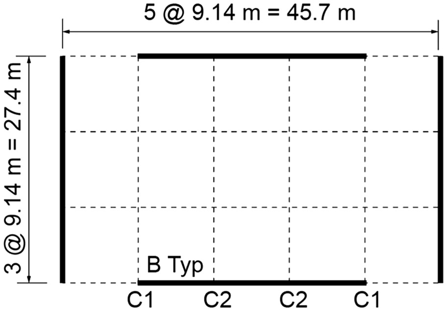
Four-, 6-, and 8-story buildings were considered in the study. The building plan and story height were the same for all and matched those used by Erochko et al. (2011). Fig. 1 shows the plan, with a 3-bay SMF on each side, a bay length of 9.1 m, and a story height of 3.7 m.

Fig. 1. Building plan geometry and member designations.

The seismic weight for the buildings was

4.3 kN / m^{2}

(

3.6 kN / m^{2} dead load + 0.72 kN / m^{2}

partitions). The

3.6 kN / m^{2}

dead load was based on

0.72 kN / m^{2}

steel frame weight;

2.0 kN / m^{2}

floor weight;

0.5 kN / m^{2}

mechanical, electrical, plumbing, insulation, lights, ceiling, floor covering;

0.2 kN / m^{2}

exterior wall weight (distributed); and

0.2 kN / m^{2}

miscellaneous. The floor was considered to extend 0.3 m past the frame lines.

The Los Angeles site used for the study was the same as in Erochko et al. (2011). The DE spectra had

S_{D S} = 1.4

and

S_{D 1} = 0.75

. The MCE spectra were 1.5 times the DE spectra.

Risk Categories and Design Criteria

Buildings were designed for Risk Categories II and IV following requirements in ASCE 7 (ASCE 2016), AISC 341 (AISC 2016b), and AISC 358 (AISC 2016a). The Risk Category II buildings were designed with an importance factor of 1.0 and a drift limit of 2.5% (4-story buildings) or 2.0% (6- and 8-story buildings). The Risk Category IV buildings were designed with an importance factor of 1.5 and a drift limit of 1.5% (4-story buildings) or 1.0% (6- and 8-story buildings). The maximum beam size was limited to

W 36 \times

. The maximum column size was limited to

W 24 \times

for Risk Category II designs and

W 27 \times

for Risk Category IV.

SMF Designs

Three different SMF connections were considered in the study, the reduced beam section (RBS) and two proprietary connections that were designated PropA and PropB (these designations were used to avoid the commercial tradenames in the academic work).

All of the SMF connections in the study were prequalified connections in AISC 358 (AISC 2022). RBS connections have been investigated in many experimental and analytical studies [see Montuori (2015) for a review] and were included in the original edition of AISC 358 (AISC 2005). The proprietary connections, PropA and PropB, have also been thoroughly vetted through experimental testing and are included in AISC 358 (AISC 2022) in Chapters 11 and 15, respectively. Experimental results for PropA are given in various test reports [see references in AISC 358 (AISC 2022)]. Experimental results for PropB are in the peer-reviewed literature (Richards 2019, 2021, 2022) and in reports referenced in AISC 358 (AISC 2022).

RAM Structural System (Bentley 2021) was used to design the frames and perform design checks (stiffness, strength, seismic provision requirements). RAM has built-in features to specifically assist with the design of RBS, PropA, and PropB connections. For the proprietary systems, the connections were modeled and checked according to the recommendations given by the connection distributors (Bentley 2021). Frames were analyzed using linear modal response spectrum analysis (ASCE 2016). The different connections resulted in different optimum beam and column sizes. For example, PropA frames used smaller beams, since substantial connection plates would be added at the beam ends, and PropB frames could use beams with higher width-to-thickness ratios than the others, because they do not form plastic hinges (AISC 2022). Also, the maximum moment that developed at the face of the column varied for the different connections, influencing the strong-column weak-beam checks. While the beam and column sizes varied depending on the connection, the stiffness of all the frames of the same height and risk category were essentially the same, reflecting the drift-governed designs. The combination of three building heights, two risk categories, and three SMF connections resulted in 18 unique frames. Table 1 summarizes the frame weights and other properties. The Appendix reports the member sizes for the frames.

Table 1. Building frame characteristics

Frame	Frame weight^a (kN)				Natural period (s)		Strength
Frame	Column	Beam	Cover Pl.	Total	RAM	OS^b	$V_{d} / W$ ^c	$V_{y} / W$ ^d
4-story
RBS II	330	427	N/A	756	1.39	1.38	0.108	0.168
RBS IV	451	625	N/A	1,080	0.96	0.96	0.162	0.315
PropA II	282	312	149	743	1.41	1.37	0.108	0.157
PropA IV	368	507	269	1,140	1	0.97	0.162	0.278
PropB II	282	368	73	723	1.42	1.39	0.108	0.113
PropB IV	356	509	98	963	1.03	0.97	0.162	0.237
6-story
RBS II	677	782	N/A	1,460	1.78	1.71	0.078	0.148
RBS IV	1,170	1,510	N/A	2,680	1	0.99	0.156	0.416
PropA II	492	620	315	1,430	1.76	1.71	0.078	0.133
PropA IV	853	1,060	625	2,540	1.02	1.01	0.156	0.334
PropB II	498	676	129	1,300	1.73	1.7	0.078	0.108
PropB IV	765	1,370	244	2,380	1.02	1.02	0.156	0.315
8-story
RBS II	884	1,000	N/A	1,900	2.4	2.36	0.062	0.103
RBS IV	2,170	1,930	N/A	4,110	1.27	1.22	0.093	0.3
PropA II	767	772	381	1,930	2.41	2.32	0.062	0.093
PropA IV	1,340	1,500	905	4,110	1.28	1.26	0.093	0.294
PropB II	718	895	155	1,780	2.43	2.36	0.062	0.067
PropB IV	1,260	1,960	342	3,570	1.28	1.26	0.093	0.245

Note: N/A = not applicable.

a

Frame weight as reported by RAM includes columns, beams, and cover plates (Cover Pl.) for PropA and PropB connections. It does not include RBS connection plates (doubler plates, continuity plates) or other connection plates for PropA and PropB connections.

b

OpenSees model used for RHA.

c

V_{d}

is the design base shear (used for strength checks). The ratio

V_{d} / W

is equivalent to

C_{s}

used for design.

d

V_{y}

is the base shear corresponding to first yield under a first-mode pushover analysis. The ratio

V_{y} / W

is an indication of actual frame strength.

Table 1 indicates weight savings for proprietary systems compared with RBS. The RBS frames had lower stiffness efficiency because of the beam cut-outs and higher panel zone flexibility. Even with added connection weight, the PropA and PropB frames generally had overall weight reductions while providing the same stiffness. The proprietary design weights were up to 13% less than the RBS weights for comparable frames, with the least total weight in the PropB frames.

The impact of risk category on total frame weight can be observed from Table 2. For the 4-story frames, the Risk Category IV SMF designs were 1.3–1.5 times heavier than the comparable Risk Category II designs. For the 6- and 8- story frames, the Risk Category IV designs were 1.8 to 2.2 times heavier than the comparable Risk Category II designs. The increased weights were due to stricter drift limits in combination with the period shift (which increased the forces required for the drift checks).

Table 2. Steel weights and total building cost index for RBS designs

Stories	Risk	$W_{S M F}$ ^a (kN)	$W_{g r a v}$ ^b (kN)	$W_{t o t}$ ^c (kN)	Total building cost index^d
4	II	756	841	1,600	1.00
4	IV	1,080	841	1,920	1.04
6	II	1,460	1,290	2,750	1.00
6	IV	2,680	1,290	3,970	1.09
8	II	1,890	1,760	3,650	1.00
8	IV	4,430	1,760	6,180	1.14

a

Total steel weight of the four SMFs in the building.

b

Total steel weight of non-SMF gravity steel framing in the building.

c

Total steel weight (

W_{S F M} + W_{g r a v}

).

d

The total building cost index was

0.8 + (0.2) \times (W_{t o t} / W_{t o t, II})

, where

W_{t o t, II}

= total steel weight from the corresponding Risk Category II design. The total building cost index is based on the following assumptions: the total steel cost for Risk II designs is 10% of the total cost of the building; the total foundation cost for Risk II designs is 10% of the cost of the building; the total steel cost is proportional to the steel weight; and the foundation costs for SMF rise in the same proportion as the steel costs for SMFs.

The cost impact of Risk Category IV design for SMFs is higher than what has been reported in more general studies. NIST (2021) suggests that designing for Risk Category IV represents less than a 2% cost premium for a building. This seems to be based primarily on buildings that were strength governed (NIST 2021). For the drift-governed RBS designs in this study, the direct structural cost premium for Risk Category IV was 4%–14% (Table 2), with the greater premiums for the taller buildings in which the seismic steel was a higher percentage of the overall steel weight. This estimate does not include the indirect effects of using deeper beams and columns (without which no feasible Risk Category IV designs could be found), which may increase costs by another 1%–2% since greater story heights would be required to attain the same floor-to-ceiling heights (not accounted for in this study).

Frame Modeling

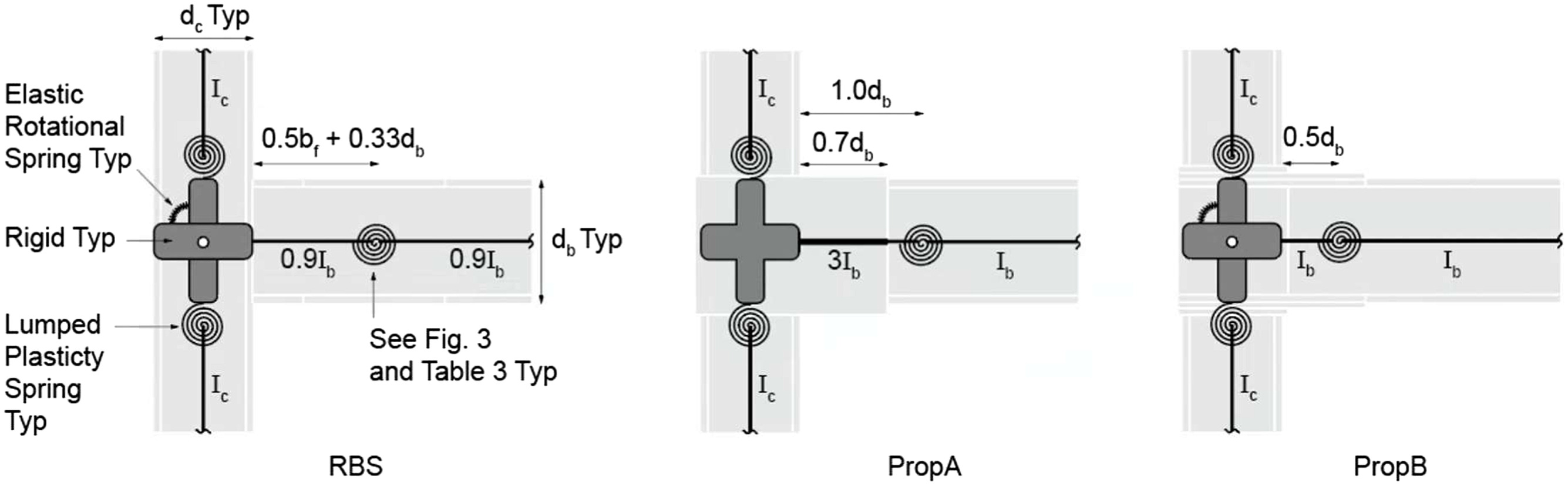
Two independent models were developed for each frame. An elastic model was generated by RAM (Bentley 2021) and used to proportion the members with modal response spectrum analysis and perform code checks, as discussed in the previous section. A nonlinear model was developed in OpenSees version 3.3.0.1.1 (Mazzoni et al. 2006) for pushover and RHA.

In the OpenSees model, beams and columns were represented with Timoshenko Beam-Column elements and lumped plasticity springs. An effective flexural stiffness was used for the beams and columns, so that less-than-infinite elastic stiffness could be assigned to the lumped plasticity springs (Zareian and Medina 2010). For determining the shear stiffness of the Timoshenko beam and column elements, the shear area was taken as the web area, measured to the centroids of the flanges.

Fig. 2 illustrates the how the joint regions were represented for each type of connection in OpenSees. For the RBS frames, a reduced moment of inertia was used for the beams (90% of actual) to represent the stiffness reduction from the cutouts (Hamburger et al. 2016). The PropA and PropB frames were simulated following the recommendations given by the proprietary connection distributors. Where panel zone scissor springs were used, they followed the recommendations from Charney and Marshall (2006), which resulted in elastic panel zone stiffness equivalent to that of a Krawinkler model.

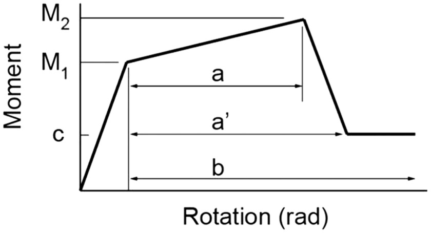
Fig. 2. OpenSees joint modeling for the different SMF connections.

The lumped plasticity beam springs in the models had backbone curves of the type shown in (Fig. 3). Table 3 summarizes the values for the spring parameters that were used for the different connections, and subsequent paragraphs explain the sources for the parameters. The OpenSees bilin material model, which simulates the modified Ibarra-Medina-Krawinkler deterioration model (Ibarra et al. 2005), was used to assign the lumped plasticity spring properties in the OpenSees models.

Fig. 3. Definition of backbone parameters for SMF beam lumped plasticity springs.

Table 3. Values for backbone parameters for lumped plasticity springs

Backbone parameter	Connection type
Backbone parameter	RBS	PropA	PropB
$a$	0.04	0.05	0.045
$a^{'}$	0.045	0.065	0.065
$b$	0.06	0.09	0.08
$c$	$0.2 M_{p}$	$0.4 M_{p}$	$0.5 M_{p}$
$M_{1}$	$0.72 M_{p}$	$1.0 M_{p}$	$0.6 M_{p}$
$M_{2}$	$0.83 M_{p}$	$1.2 M_{p}$	$1.0 M_{p}$

The backbone parameters for the RBS springs were taken from ASCE 41 (ASCE 2017) and AISC 358 (AISC 2016a). ASCE 41 gives values for

a

,

b

, and

c

(defined in Fig. 3) in terms of beam depth. A beam depth of 0.91 m was used to determine the values in Table 3, based on the deepest beams used in the designs. The RBS

M_{1}

value of

0.72 M_{p}

was based on the ratio of the plastic section modulus of the RBS regions to that of the unreduced beams, which ranged from 0.72 to 0.73 for the designs. The RBS

M_{2}

value was based on a

C_{p r}

value of 1.15 [

1.15 (0.72) = 0.83

] (AISC 2016a).

The backbone parameters for the PropA springs were determined from experimental results given in Fig. C-11.1(b) of AISC 358 (AISC 2016a), adjusted to reflect the more common bolted configuration. The values for

a

and

b

suggested by Fig. C-11.1(b) of about 0.04 and 0.08 were increased to 0.05 and 0.09 to account for beneficial bolt slip, not present in the experiment for Fig. C-11.1(b) but present in current bolted configurations. The

M_{1}

and

M_{2}

values of about

1.0 M_{p}

and

1.2 M_{p}

from Fig. C-11.1(b) would be similar for both bolted and welded configurations. The residual strength ratio suggested by Fig. C-11.1(b) was 0.4.

The backbone parameters for the PropB springs were derived by McCall and Richards (2020), based on prequalification experiments (Richards 2022). Relative to the RBS,

M_{1}

was lower for the PropB springs, but the maximum moment

M_{2}

was higher, due to the shear yielding mechanism in the PropB connections that enables them to reach high strains without local buckling.

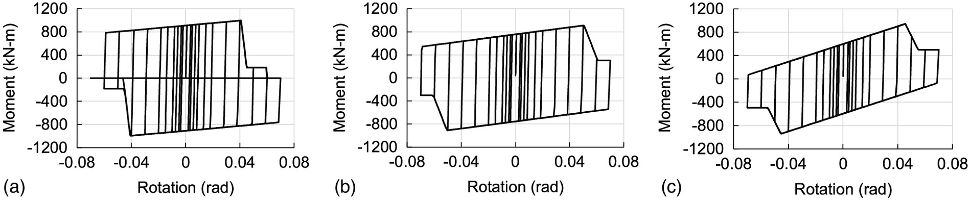
Fig. 4 compares the hysteretic behavior of the springs for the beams in first story of the 4-story Risk Category II buildings. In each case, the inelastic spring was subjected to the loading protocol in AISC 341 (AISC 2016b), Chapter K. Note that hinge ultimate strengths were similar for all, despite the higher

M_{1}

and

M_{2}

for PropA in Table 3, because the RBS and PropB designs use heavier beams (Appendix). The PropB hysteretic behavior is characterized by lower initial yield force and higher postyield stiffness.

Fig. 4. Lumped plasticity spring validation plot for first-story beams in the 4-story Risk Category II frames: (a) RBS, $W 24 \times 84$ ; (b) PropA, $W 24 \times 55$ ; and (c) PropB, $W 24 \times 62$ .

Simpler lumped-plasticity springs were used for the columns (Fig. 2), in which less inelasticity was expected and realized. The column springs were modeled in OpenSees with steel01 material with 2% strain hardening.

All of the OpenSees frame models had a leaning column to represent the gravity framing and

P - Δ

effects associated with each frame. The leaning column was pinned at the base and constrained to match the displacement of the SMF at each floor level. The effective moment of inertia for the leaning column varied every two stories, corresponding to the gravity column splices, and ranged from

9.82 \times 10^{8}

to

2.11 \times 10^{8} {mm}^{4}

. The seismic mass for the model was assigned to nodes on the leaning column,

285 kN - s^{2} / m

at each level, corresponding to half of the mass of each floor (since there were two frames in each direction). A downward force of 3,203 kN at each level was applied to the leaning column to represent the gravity loads (

1.2 D + 0.5 L

) associated with half of each floor.

Eigenvalue and Pushover Analysis

The building periods from the RAM models were used to validate the elastic behavior of the OpenSees models. Table 1 shows that OpenSees periods were similar those from RAM. The reasons for the small discrepancies in natural period between RAM and OpenSees varied for the different connections. For the RBS connections, RAM represented the cut sections with dedicated elements, while in OpenSees a general penalty on the beam stiffness was applied (Fig. 2). For RBS panel zones, a partial rigid end offset was used in RAM, while a scissor spring was used in OpenSees. For PropA frames, RAM used a proprietary database with beam-dependent parameters when representing the joints, while in OpenSees, parameters relative to beam depth (Fig. 2) were applied. Overall, the similar periods from RAM and OpenSees confirmed reasonable modeling of the elastic stiffness.

Comparing periods across different designs, the natural periods were similar for frames with the same height and risk category, reflecting that they were all designed for the same drift limit. For the 4-story frames, natural periods were around 1.4 s for Risk Category II and 1.0 s for Risk Category IV. The 6-story frames had periods similar to the 4-story frames, because the effects of the increased height were offset by the stricter design drift limit. For 8-story frames, natural periods were around 2.4 s for Risk Category II and 1.2 s for Risk Category IV.

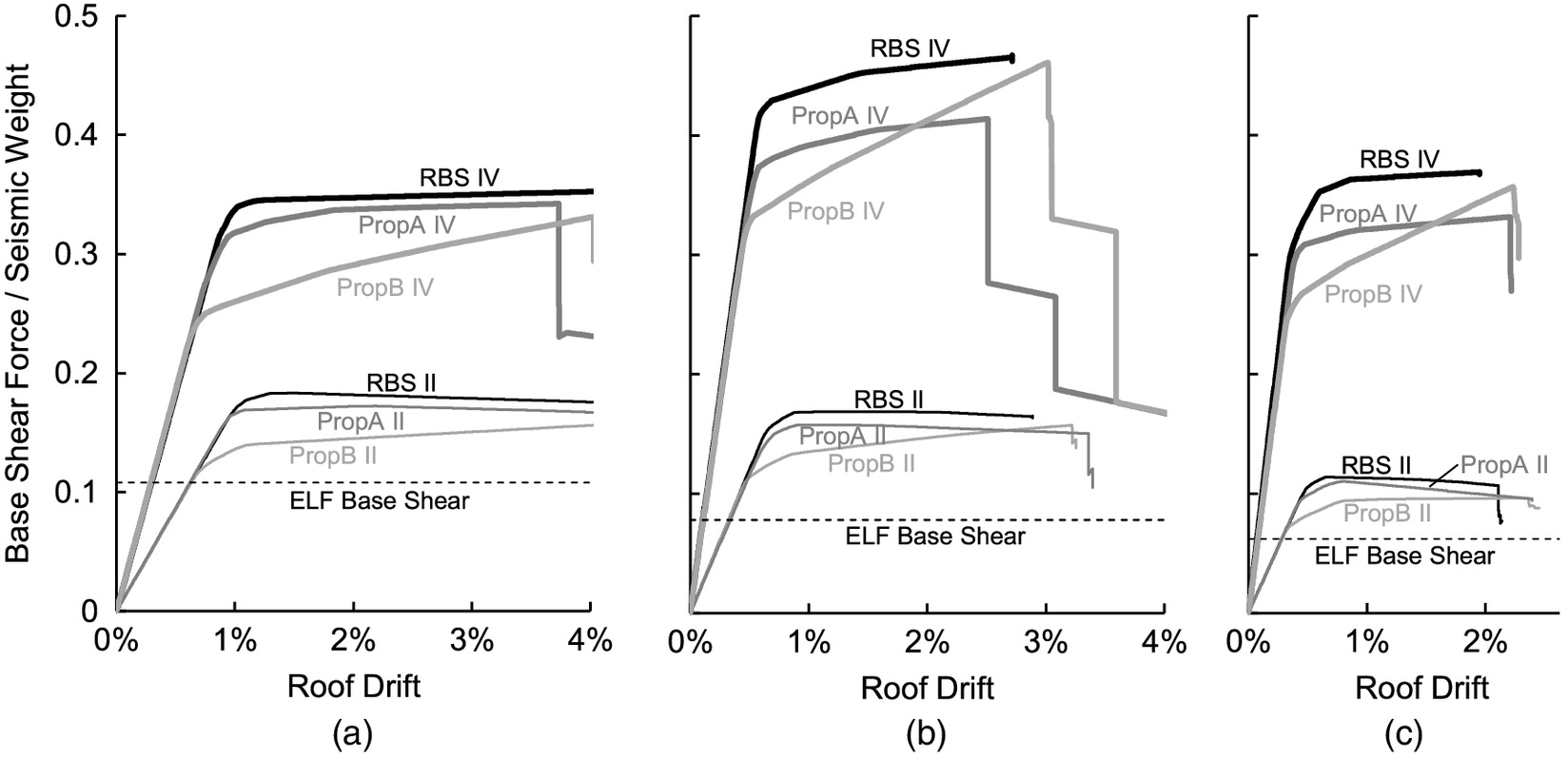
Pushover analysis was performed as part of the validation of the OpenSees models. The results shown in Fig. 5 have limited pertinence beyond basic validation, since an equivalent lateral force (ELF) distribution was used, and inelasticity concentrated in the lowest stories. The yield strength in all cases was higher than the ELF base shear (Fig. 5), reflecting drift-governed design. For a given frame height and risk category, RBS designs had the highest yield strength and PropB the lowest. However, PropB designs had greater postyield stiffness (5%), as would be expected based on the backbone parameters for the beam hinges (Figs. 3 and 4), and had strength similar to the RBS and PropA frames at high drifts. The difference in stiffness between the Risk Category II and IV designs was consistent with the design basis. For example, the 8-story Risk Category IV designs had 3.9 times greater initial stiffness than the Risk Category II designs, consistent with the drift limit reduction (factor of 2) and shift in actual building period (additional factor of 1.9).

Fig. 5. Pushover analysis results: (a) 4-story; (b) 6-story; and (c) 8-story.

Response History Analysis

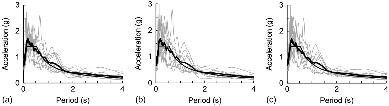
Ground motions were selected and scaled following procedures in ASCE 7 (ASCE 2016). Because RHA was performed on individual frames, individual components of records were considered, rather than pairs. Eleven ground motions were chosen from the FEMA P695 far-field suite and scaled so that the average spectra would not fall below 90% of the spectrum in the range of interest. Different scale factors were used for the 4-, 6-, and 8-story buildings, since the period range varied for each group (Table 4). Fig. 6 illustrates the scaled and average spectra for the DE. The MCE design spectra and scaled records are equal to 1.5 times the DE. The acceleration records were padded with 60 s of zero acceleration at the end to allow the frames to come to rest so that residual drifts could be evaluated.

Table 4. Earthquake records and scaling factors for RHA

GM no.	Event	Recording	PEER-NGA record no.	DE scale factor
GM no.	Event	Recording	PEER-NGA record no.	4-story	6-story	8-story
1	Hector Mine, 1999	HECTOR/HEC000	1,787	3.02	3.35	3.34
2	Imperial Valley, 1979	IMPVALL/H-DLT262	169	2.47	2.39	2.23
3	Kobe, Japan, 1995	KOBE/SHI000	1,116	2.90	3.11	2.77
4	Kocaeli, Turkey, 1999	KOCAELI/DZC180	1,158	2.10	2.13	2.01
5	Kocaeli, Turkey, 1999	KOCAELI/ARC090	1,148	3.87	3.66	3.50
6	Landers, 1992	LANDERS/YER360	900	3.46	3.09	3.16
7	Manjil, Iran 1990	MANJIL/ABBAR—T	1,633	1.34	1.42	1.27
8	Superstition Hills, 1987	SUPERST/B-ICC000	721	2.47	2.23	2.54
9	Superstition Hills, 1987	SUPERST/B-POE360	725	2.48	2.85	2.72
10	Chi-Chi, Taiwan, 1999	CHICHI/CHY101-E	1,244	1.57	1.54	1.41
11	San Fernando 1971	SFERN/PEL090	68	2.58	2.22	3.41

Fig. 6. Scaled earthquake spectra for the DE (a) 4-story; (b) 6-story; and (c) 8-story.

Rayleigh damping was used in the models to represent inherent damping in the structure. Stiffness proportional damping was assigned only to the linear beam and column elements (Zareian and Medina 2010). Mass proportional damping was assigned only to the nodes with point masses. Mass and stiffness multipliers were based on 2% damping in Modes 1 and 3.

Each of the frames was analyzed under the suite of earthquakes scaled to the DE level and again for the suite scaled to the MCE level. The SmartAnalyze script (Dong 2019) was used to automatically adjust time increments and solution methods to maximize the likelihood of completing the analyses.

Floor displacements and accelerations were output at each time increment. Maximum story drifts (peak and residual) and floor accelerations (absolute) were determined, and then mean and median values over the entire suite were calculated as final results and as inputs for FEMA P-58 analysis.

FEMA P-58 Analysis

The software SP3 RiskModel (HBR 2022) was used to perform the FEMA P-58 analysis (ATC 2019). The component fragility functions for the RBS connections were developed by Deierlein and Victorsson (2008) in accordance with the FEMA P-58 method for fragility creation. The fragility functions for PropA and PropB were developed independently by HBR with the same methods, using laboratory tests reports to define the connection behaviors and using the RBS fragility curves as a benchmark [e.g. (HBR 2020a)]. Table 5 summarizes some of the fragility and loss parameters for the connections that were used for the loss analysis. The parameters in Table 5 were for a one-sided connection with a beam depth of 0.69 m or less (HBR 2022). Repair costs were lowest for PropB, because the connection incorporates replaceable fuses. Parameters for two-sided connections and deeper beams were developed in the same way.

Table 5. Fragility and loss parameters for SMF connections

Fragility group	Damage state	Fragility parameters		Repair cost parameters^a			Repair time parameters
Fragility group	Damage state	Drift (%)^b	$β$	$C_{\max}$ ($K)	$C_{\min}$ ($K)	$β$	$T_{\max}$ (d)	$T_{\min}$ (d)	$β$
RBS (B1035.001)	DS1	3.0	0.30	21.7	14.8	0.35	12.8	8.7	0.43
	DS2	4.0	0.30	36.6	24.9	0.31	21.5	14.7	0.39
	DS3	5.0	0.30	36.6	24.9	0.31	21.5	14.7	0.39
PropA (B1035.201)	DS1	4.6	0.34	17.0	11.4	0.37	10.2	6.7	0.42
	DS2	5.5	0.34	20.9	13.9	0.36	12.3	8.2	0.42
	DS3	5.9	0.34	29.3	19.6	0.36	17.3	11.5	0.41
	DS4	7.6	0.79	29.3	19.6	0.37	17.3	11.5	0.41
PropB (B1035.301a)	DS1	6.0	0.33	10.9	7.4	0.35	6.4	4.4	0.43
PropB (B1035.301a)	DS2	9.0	0.33	14.4	9.8	0.29	8.5	5.8	0.38

a

Repair costs are shown in 2011 dollars. Scale factors were applied to these values based on the ratio of current/2011 expected building replacement cost.

b

Residual drift.

The fragility functions in Table 5 specifically relate to circumstances in which the residual drifts are low enough that building repair is feasible. The feasibility of repair is evaluated separately based on residual drifts. For RBS and PropA buildings, the buildings were considered not repairable if residual drifts exceeded 1% (ATC 1997; HBR 2020a). For PropB, special residual drift fragility parameters that reflect the improved repairability of the connection, which had been developed previously (Table 6) (HBR 2020a), were used when residual drifts were high.

Table 6. Fragility and loss parameters for residual drift repair of PropB frames

Fragility group	Damage state	Fragility parameters		Repair cost parameters^a			Repair time parameters
Fragility group	Damage state	Res. drift (%)	$β$	$C_{\max}$ ($K)	$C_{\min}$ ($K)	$β$	$T_{\max}$ (d)	$T_{\min}$ (d)	$β$
PropB (B1100.301)	DS1	1.0	0.30	68.3	46.5	0.36	43	29	0.39
	DS2	2.0	0.30	72.0	48.9	0.35	48	32	0.39
	DS3	2.5	0.30	75.6	51.4	0.35	52	36	0.39

Note: Res. drift = residual drift.

a

Repair costs are per frame line and are shown in 2011 dollars. Scale factors were applied to these values based on the ratio of current/2011 expected building replacement cost.

The fragility parameters and quantities for the other components of the buildings were the defaults assumed by SP3 RiskModel (HBR 2022) based on the square footage of the buildings. The components that were considered in the loss estimate were bolted shear tabs (B1031.001), column base plates (B1031.011a), column splices (B1031.021a), steel moment connections (Table 5), precast concrete panels (B2011.201), curtain walls (B2022.002), wall partitions (C1011.001b), steel stairs (C2011.011b), wall partition finishes (C3011.001b), raised access floor (C30127.002), suspended ceiling (C3023.003a-d), independent pendant lighting (C3034.002), elevator components (D1014.041-.044), potable water piping and bracing (D2021.013a-b; D2021.023a-b), sanitary waste piping (D2031.013b), chiller (D3031.013c), HVAC (D3041.011c, D3041.032c, D3041.103c, D3052.013f, D3067.012c), fire sprinkler piping and drop (D4011.024a, D4011.054a), transformer/primary service (D5011.013c), motor control centers (D5012.013d), low voltage switchgears (D5012.023c), and distribution panels (D5012.033c). Components (stairs, ceilings, lighting, piping, HVAC, and electrical equipment) were all assumed to be seismically rated.

The median drifts (maximum and residual) and floor accelerations from the RHA were used as the demand input parameters for the P-58 analysis. This approach is more precise than using the drifts and accelerations estimated by SP3 RiskModel (when RHA is not performed).

The outputs from the P-58 analysis were expected repair costs and time to achieve functional recovery. Expected repair costs were output as a percentage of the building replacement value. The functional recovery repair time was computed using the ATC-138 Functional Recovery Assessment Methodology (Beta) (ATC 2021). The SP3 RiskModel assumptions for functional recovery were HVAC functional, elevator functional, no more than 3 stories requiring stair access, and no surge demand. Impeding factors on the functional recovery repair time were inspection, financing, permitting, engineering mobilization, and contractor mobilization. For buildings that were not repairable (residual drifts exceeded the threshold), the functional recovery repair time was equal to the total rebuild time.

Results

The results from the study are presented in three parts: first, the results from the RHA under DE-scaled earthquakes; then, the RHA results for MCE shaking; and finally, the results from the FEMA P-58 analysis.

DE Results

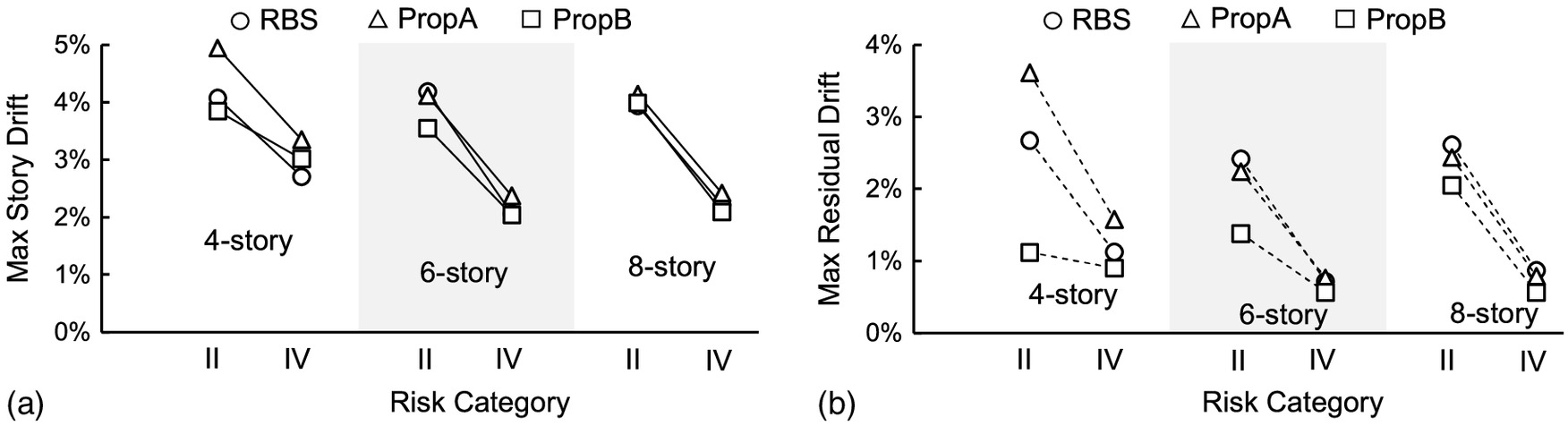
Maximum and residual drifts from the DE analyses are presented in Fig. 7. Each plot shows the results for Risk Category II (lighter lines) and Risk Category IV (heavier lines) designs with a particular connection. Solid lines indicate maximum drifts, and dashed lines indicate residual drifts. The plots for the 4-story frames are at the top, 6-story in the middle, and 8-story at the bottom. The plots for the RBS frames are at the left (data points indicated with circles), PropA frames in the middle (triangles), and PropB frames on the right (squares).

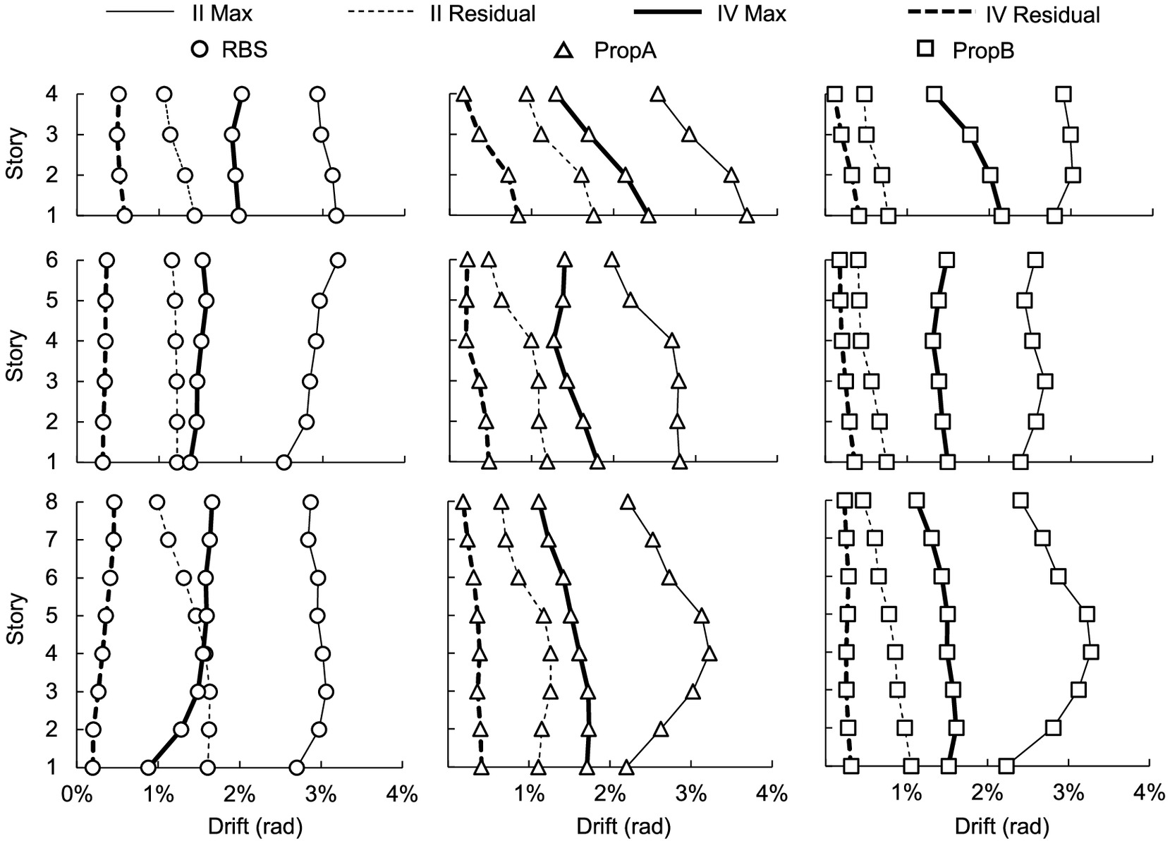
Fig. 7. Mean DE story drifts for frames in Risk Category II (light lines) and Risk Category IV (heavy lines).

The Risk Category II RBS designs are discussed first, as they represent baseline cases for the study. For RBS Risk Category II designs (Fig. 7, left column, light solid lines), the DE story drifts were around 2.5%–3%, which was a little greater than what was predicted by the linear modal response spectrum used in design. For RBS Risk Category II designs, the peak residual drifts from the different building heights ranged from 1.2% to 1.6% (Fig. 7, left column, light dashed lines), exceeding the 1.0% threshold and indicating the frames may be a total loss. The maximum and residual drifts for the Risk Category II RBS designs were consistent with those reported in other SMF studies (Erochko et al. 2011; Harris and Speicher 2018).

Results for the Risk Category IV RBS designs are shown on the same plots (Fig. 7, left column) with heavy lines. Designing for Risk Category IV reduced maximum drifts by around 1% drift, consistent with the design intent, and reduced residual drifts by a factor of two or more. For the 4-story frames, residual drifts were still above 0.5% even with the Risk Category IV design. However, the Risk Category IV designs for the 6- and 8- story frames had residual drifts under the 0.5 threshold (Fig. 7, left column).

For Risk Category II PropA designs (Fig. 7, middle column, lighter lines), the maximum drifts were around 2.8%–3.6%, a little worse than the RBS frames. The maximum residual drifts ranged from 1.1% to 1.8%. The higher drifts for PropA designs, relative to RBS, may be due to the lighter columns (Table 10). The Risk Category IV PropA designs (Fig. 7, middle column, heavier lines) were effective in reducing residual drifts, however they were still above 0.5% for the 4-story frame.

For Risk Category II PropB designs (Fig. 7, right column, lighter lines) the maximum drifts were around 2.5%–3.4%, similar to the RBS and PropA. The Risk Category II PropB maximum residual drifts ranged from 0.8% to 1.0%, much better than the RBS designs, even though the columns and beams were lighter. This can be attributed to the greater postyield stiffness in the PropB connections and is consistent with results from other studies of systems with higher postyield stiffness (Pettinga et al. 2007). The Risk Category IV PropB designs had the lowest residuals drifts of the frames in the study, below 0.5% for DE shaking for all frame heights.

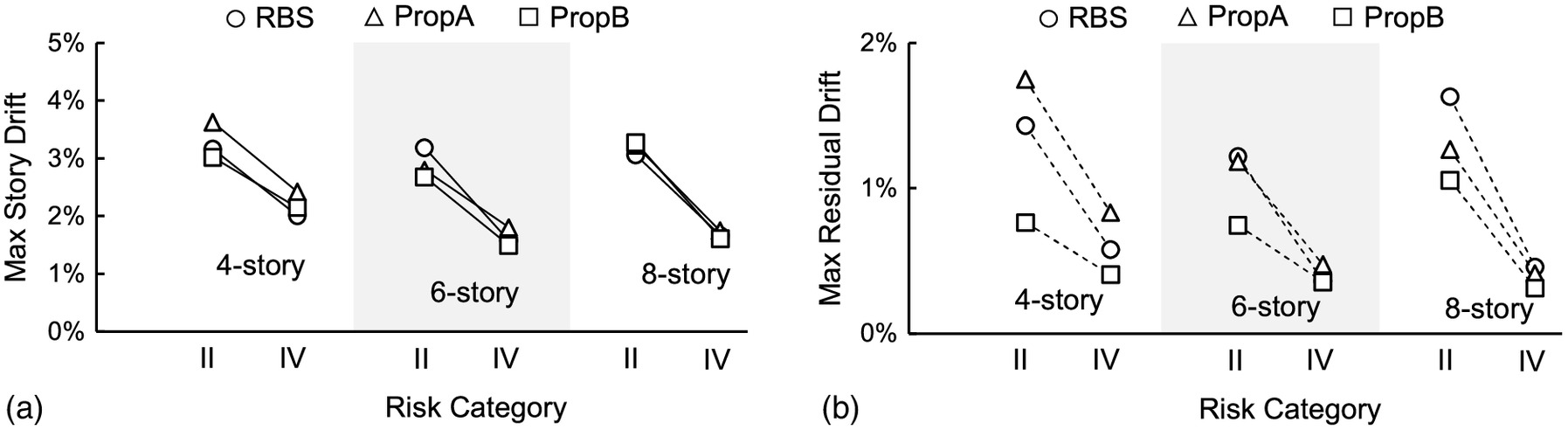
Drift results for DE are further summarized for interpretation in Figs. 8 and 9. Fig. 8 shows average results, and Fig. 9 shows the average plus one standard deviation. The general relationships between the results for the different connections (RBS, PropA, and PropB) are similar between Figs. 8 and 9, suggesting similar distribution of response. The plots highlight the more dramatic reduction in residual drift than in maximum drift for the Risk Category IV design versus the Risk Category II design. PropB frames had the lowest residual drifts for all cases.

Fig. 8. Mean DE drifts for the 11 ground motions: (a) maximum interstory; and (b) maximum residual.

Fig. 9. Mean plus one standard deviation DE drifts for the 11 ground motions: (a) maximum interstory; and (b) maximum residual.

MCE Results

None of the Risk Category II designs was able to complete all the MCE records without numerical problems, but most of the Risk Category IV designs did. Table 7 indicates which MCE analyses were able to run to completion. To make use of the available data, failed analyses were assigned a maximum drift of 10% [following Erochko et al. (2011)] and residual drift of 2%. Fig. 10 summarizes drifts from the MCE analyses, including these adjustments.

Table 7. MCE analyses that completed without numerical instability (P = passed)

Height	Risk category	Connection type	Ground motion											Pass rate (%)
Height	Risk category	Connection type	1	2	3	4	5	6	7	8	9	10	11	Pass rate (%)
4-story	II	RBS	—	P	—	—	P	—	P	—	P	—	P	45
		PropA	—	—	—	—	—	—	P	—	P	—	P	27
		PropB	P	P	P	—	—	—	P	P	—	P	P	64
	IV	RBS	P	P	P	P	P	P	P	P	P	P	P	100
		PropA	P	P	P	P	P	P	P	P	P	P	P	100
		PropB	P	P	—	P	P	P	P	P	P	P	P	91
6-story	II	RBS	—	—	—	—	P	P	P	P	P	—	P	55
		PropA	—	—	—	—	P	P	P	P	P	—	P	55
		PropB	P	P	—	—	P	P	P	P	P	—	P	73
	IV	RBS	P	P	P	P	P	P	P	P	P	P	P	100
		PropA	P	P	P	P	P	P	P	P	P	P	P	100
		PropB	P	P	P	P	P	P	P	P	P	P	P	100
8-story	II	RBS	P	—	—	—	—	—	P	—	—	—	P	27
		PropA	P	—	—	—	—	P	P	—	P	—	P	45
		PropB	P	P	—	—	—	P	P	—	P	P	P	64
	IV	RBS	P	P	P	P	P	P	P	P	P	P	P	100
		PropA	P	P	P	P	P	P	P	P	P	P	P	100
		PropB	P	P	P	P	P	P	P	P	P	P	P	100

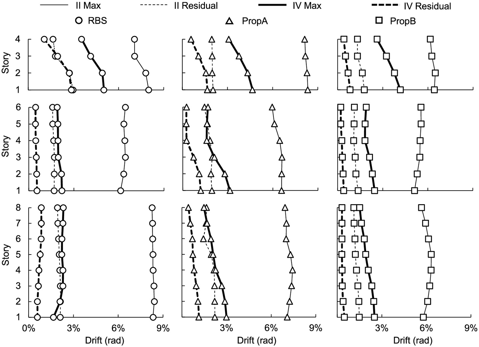
Fig. 10. Mean MCE drifts and residual drifts for Risk Category II and IV frames.

The inability of most of the Risk Category II designs to complete most of the MCE earthquakes suggests that they may not meet the collapse prevention performance objective targeted by ASCE 7. The large story drifts in Fig. 10 for the Risk Category II designs indicate questionable performance. Because incremental dynamic analysis was outside the scope of the present study, the collapse prevention performance was not rigorously evaluated. The Risk Category IV frames fared better for MCE loading, although residual drifts were greater than 0.5% in all cases except the 6- and 8-story PropB frames (Fig. 10).

FEMA P-58 Results

Results from the P-58 analysis loss analyses are shown in Figs. 11 and 12. Fig. 11(a) shows functional recovery repair costs from the DE in terms of the replacement value of the buildings. Risk Category II and IV buildings with the same height and connection type are linked. Functional recovery costs were similar for the RBS and PropA designs, ranging from 64% to 88% for Risk Category II and 14% to 57% for Risk Category IV. Functional recovery costs were much lower for the PropB connections because of lower residual drifts (Fig. 7) in combination with improved repairability (Tables 5 and 6). In fact, the functional recovery costs for the Risk Category II PropB frames were similar to those of Risk Category IV RBS and PropA frames of comparable height, even though the Risk Category II PropB frames were much lighter. For all three connections, the repair costs for the 4-story buildings were higher than for the 6- and 8- story designs because of the higher drifts (associated with the higher drift limit used in design).

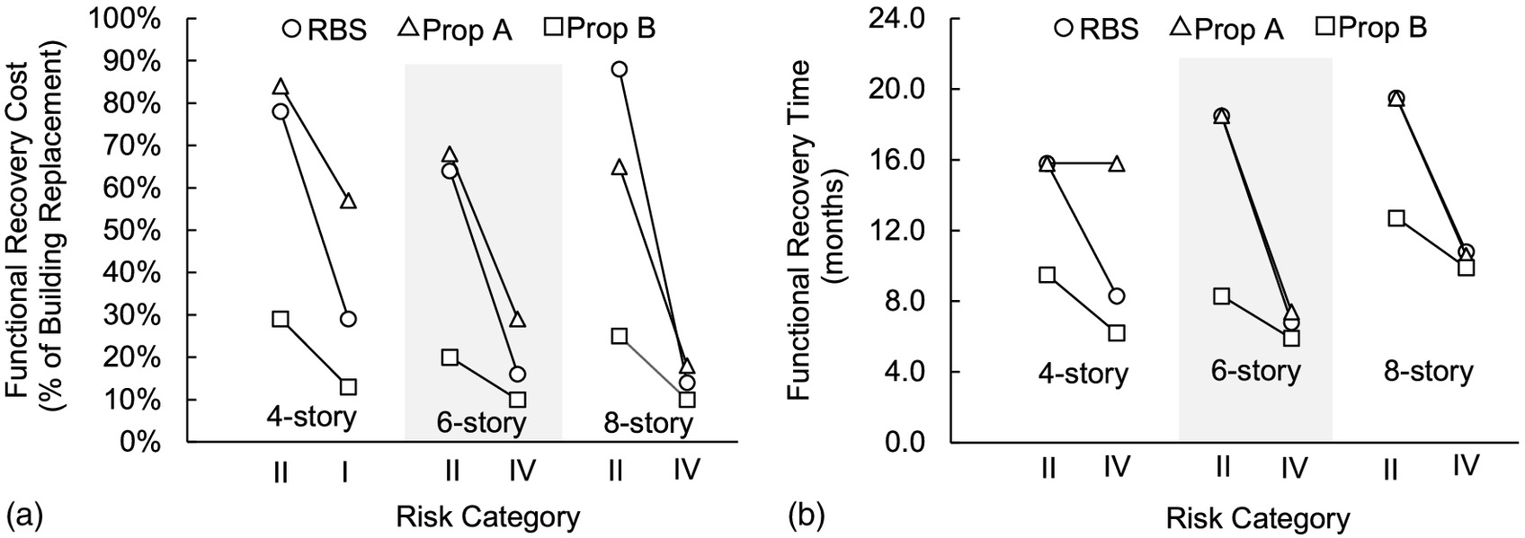
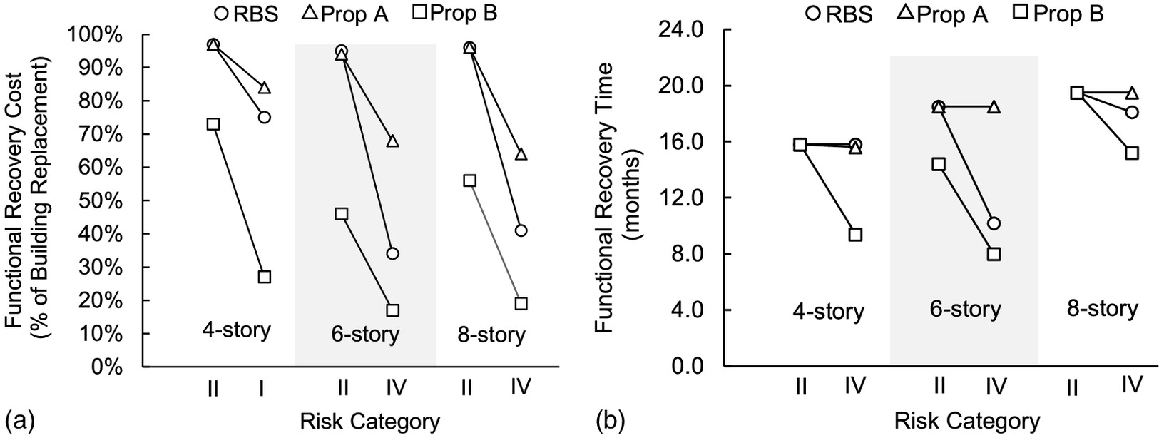
Fig. 11. DE functional recovery costs and functional recovery times from P-58 analysis.

Fig. 12. MCE functional recovery costs and functional recovery times from P-58 analysis.

Fig. 11(b) shows functional recovery repair times from the DE designs. The times for the RBS and PropA Risk Category II frames correspond to a total rebuild, triggered by the high residual drifts. The PropB Risk Category II frames had much lower functional recovery repair times compared with the RBS and PropA Risk Category II designs. Risk Category IV design reduced repair times to 6–11 months, except for the 4-story PropA frame.

Figs. 12(a and b) show results for the MCE in a similar format. The RBS and PropA Risk Category II designs would be a total loss (normalized cost of essentially 100% and a repair time equal to total rebuild). By designing for Risk Category IV, repair costs for RBS and PropA were reduced to 32%–85% of the replacement value. The PropB frames had significantly lower losses, owing to lower residual drifts (because of postyield stiffness) and improved repairability (because of replaceable fuses).

Discussion

The results are discussed in the context of previous studies and the ongoing conversation about how to incorporate functional recovery into building codes.

FEMA P-58-5 Study

The results from the present study were substantially different from a previous P-58 study that included steel SMFs designed as Risk Categories II and IV. In FEMA P-58-5 (ATC 2018), the FEMA P-58 methodology was applied to several building archetypes. Some of the building archetypes were steel SMFs, including some Risk Category II and some Risk Category IV designs. Table 8 compares results from the ATC 2018 study with the RBS results of the present study. The repair costs and repair times from the present study are much higher, even though they are functional recovery rather than full-recovery costs and times (Table 8).

Table 8. Median drifts and repair costs for nonproprietary SMFs under DE shaking from the present study and the ATC 2018 study

Risk	Height	Drift (%)		Residual drift (%)		Repair cost (% of replacement)		Repair time (mo)
Risk	Height	RHA^a	P-58-5	RHA	P-58-5	Fig. 11	P-58-5	Fig. 11	P-58-5
II	Low-rise^b	3.0	1.5–2.7	1.1	0.15–0.50	64–88	5–13	15.8–19.5	0.5–1.2
II	Mid- rise^c	2.9–3.1	1.1–1.9	0.91–1.60	0.03–0.26	64–88	5–13	15.8–19.5	0.5–1.2
IV	Low-rise	2.0	1.0–1.7	0.40	0.01–0.22	14–29	3	6.8–10.8	0.4–0.5
IV	Mid- rise	1.6–1.7	0.6–1.0	0.27–0.31	0.00–0.01	14–29	3	6.8–10.8	0.4–0.5

a

The drift ratios are for the RBS designs in the present study; median values used for the P-58 analysis are shown.

b

The 4-story frames in the present study were compared with the low-rise frames from the P-58-5 study.

c

The 6- and 8-story frames in the present study were compared with the mid-rise frames from the P-58-5 study.

The primary reason for the discrepancy is the difference in the methodology for producing the drift demands that were inputs for the FEMA P-58 analysis. In the ATC 2018 study, simplified design and analysis procedures were used to accommodate the volume of archetypes being considered. Dynamic properties of the SMFs were estimated and demands were estimated, without producing explicit frame designs or performing any frame analyses. Because the simplified elastic procedures used for “design” were essentially the same as those used for “analysis,” the drift demands were self-fulfilling. Residual drifts were roughly estimated based on the estimated maximum drifts. The exercise was an effective demonstration of how FEMA P-58 could be used, but the estimated residual drifts were not consistent with those that have been observed in studies with more rigorous SMF design and analyses (Erochko et al. 2011; Harris and Speicher 2018).

The drift demands in the present study came from frames that were explicitly designed (Appendix) and analyzed with nonlinear RHA. The results from the RHA in this study (Fig. 7) were consistent with the other studies mentioned in the ASCE 7 commentary that have recognized that SMFs designed with linear model response spectrum analysis “do not necessarily achieve the intended collapse performance” (ASCE 2016).

Impact of Drift Limits on Functional Recovery

Risk Category IV design improved functional recovery times, but they were still more than 6 months for the RBS frames. For the RBS designs, going from Risk Category II to Risk Category IV reduced functional recovery times from 15.8 to 19.5 months down to 6.8 to 10.8 months for the DE. Recovery times for PropB frames were slightly better [Fig. 11(b)]. The functional recovery times observed for the Risk Category IV frames were higher than people might guess based on other work, particularly FEMA P-58-5 (ATC 2018).

Risk Category IV design reduced functional recovery costs, but probably not enough to offset the initial higher construction costs. SMFs with traditional inelasticity (RBS and PropA), designed as Risk Category IV, saved an average of 47% of the replacement value of the building in repair costs after DE shaking relative to when they were designed as Risk Category II buildings (Fig. 11). If the DE earthquake were to occur 30 years after initial construction, the Present Value of those savings would be 7% of the replacement value (assuming 7% discount rate). These savings are less than the average initial direct cost premium for the Risk Category IV designs, which was 9% (Table 2), and the probability of the DE earthquake even occurring in 30 years is less than 10%. This crude economic analysis and the disappointing functional recovery times do not make a compelling economic argument for Risk Category IV design, even though it may be the correct policy for other reasons.

Impact of Postyield Stiffness and Connection Repairability on Functional Recovery

The higher postyield stiffness of the PropB frames resulted in reductions in residual drift compared with other systems (Figs. 7 and 8, previously discussed), even though the PropB frames were lighter (Table 1). This study confirms for SMFs what has been demonstrated for other systems, that residual drifts are most heavily influenced by postyield stiffness (MacRae and Kawashima 1997; Pettinga et al. 2007). The PropB connections also had lower repair costs and repair times, as represented in the fragility functions (Table 5).

In the FEMA P-58 analysis, the impact of both higher postyield stiffness (reduced residual drift demands) and improved repairability (improved fragility curves, reduced connection repair costs) are combined so that the effects of each component are unclear from results in Fig. 11. In other words, it is difficult to quantify how much of the improved functional recovery that is shown in Fig. 11 for Risk Category II PropB designs can be attributed to the reduction in residual drifts and how much can be attributed to improved connection repairability.

To quantify the amount of functional recovery improvement (cost/time) that could be attributed to repairability, the P-58 analyses were rerun for the PropB frames, using the drifts from the RBS frames. By comparing these results with those of the RBS frames, the fraction of the functional recovery improvement (cost/time) due to repairability was determined. The remaining functional recovery improvements (cost/time) were attributed to the lower residual drifts for the PropB frames. Table 9 indicates that 63%–82% of the repair cost improvement for the PropB frames (relative to RBS) could be attributed to improved repairability. Table 9 indicates that 28%–89% of the repair time improvement for the PropB frames (relative to the RBS) could be attributed to improved repairability.

Table 9. Percentage of PropB repair reductions (relative to RBS) attributed to better repairability and lower residual drifts

Height	Risk category	Repair cost reduction		Repair time reduction
Height	Risk category	Due to repairability (%)	Due to lower residual drifts (%)	Due to repairability (%)	Due to lower residual drifts (%)
4-story	II	82	18	89	11
4-story	IV	81	19	52	48
6-story	II	82	18	84	16
6-story	IV	67	33	33	67
8-story	II	63	37	28	72
8-story	IV	75	25	44	56

Most of the functional recovery benefits that could be obtained from Risk Category IV design for RBS and PropA frames could be obtained with no initial cost premium by using a Risk Category II PropB frame. The economic loss of the PropB Risk Category II frames was similar to that of the RBS Risk Category IV frames (Fig. 11), despite the RBS Risk Category IV frames being 1.3–2.2 times heavier (Table 1) and 2.2–3.9 times more stiff (Fig. 5).

As researchers and code-writers consider measures to incorporate functional recovery into building codes, it is important to recognize that postyield stiffness—not building strength or elastic stiffness—is the most important parameter for controlling residual drifts in buildings, and that repairability for residual drifts over 1% needs to be addressed.

Summary and Conclusions

Current SMF design practice for Risk Category II will result in buildings that require repair or are a total loss after DE shaking. The objective of the present study was to use FEMA P-58/ATC-138 to quantify the functional recovery impact for SMFs designed as Risk Category IV and/or using proprietary connections. The motivation for the study was to identify the most economical path toward SMF functional recovery.

RHA was performed on 18 SMFs designed with different heights (4, 6, and 8 stories), different risk categories (II and IV), and different connections [RBS and two proprietary connections (PropA and PropB)]. One of the proprietary connections (PropB) had enhanced postyield stiffness and repairability. Story drift results and floor accelerations from the RHA analyses under DE and MCE loading were used in FEMA P-58 loss analyses to evaluate the functional recovery repair costs/times for the various designs. The study supports the following conclusions about low- and mid-rise SMFs designed using linear modal response spectrum analysis.

Conclusions from the SMF building designs:

•

Six- and 8-story SMFs designed for Risk Category IV were 1.8–2.2 times heavier than Risk Category II designs and required deeper beams and columns.

•

The direct cost premiums for Risk Category IV design (versus Risk Category II) were 4%–14% of the total building costs, with the greatest cost premiums for the 8-story buildings.

Conclusions from the RHA analyses:

•

SMFs with traditional inelasticity (RBS and PropA), designed with linear modal response spectrum analysis, were questionable for life safety at DE and collapse prevention at MCE. The Risk Category II SMFs with RBS connections had residual drifts above 1% for DE loading and could complete fewer than 55% of MCE simulations.

•

Four-story SMFs with traditional inelasticity (RBS and PropA), designed as Risk Category IV, still had DE residual drifts from RHA that were greater than the 0.5% threshold.

•

SMFs with enhanced postyield stiffness (PropB) had similar maximum drifts but lower residual drifts than SMFs with traditional inelasticity (RBS and PropA).

Conclusions from the FEMA P-58 analyses:

•

SMFs with enhanced postyield stiffness and repairability (PropB), designed as Risk Category II, had functional recovery repair costs/times comparable to those of the much heavier Risk Category IV designs with traditional inelasticity (RBS and PropA).

•

SMFs with traditional inelasticity (RBS and PropA), designed as Risk Category IV, saved an average of 47% of the replacement value of the building in repair costs after DE shaking relative to when they were designed as Risk Category II buildings, but those savings were insufficient to offset the higher initial construction costs (taking into account time value of money), unless the earthquake occurred within the first 30 years.

•

SMFs with enhanced postyield stiffness and repairability (PropB), designed as Risk Category IV, had the fastest DE function recovery times, but those recovery times were still 5.9–9.9 months.

•

The best functional recovery repair costs and times were achieved when enhanced postyield stiffness and repairability were combined with Risk Category IV design. However, the higher costs associated with Risk Category IV design make it difficult to justify with economic analysis.

•

FEMA P-58 results were highly sensitive to the drift demands. Results from this study, in which drifts demands were determined through RHA, were significantly different from results of a previous study in which drift demands were simply estimated.

Recommendations for code development:

•

The 2.5% drift limit in ASCE 7, for Risk Category II buildings that are 4 stories or less, should be reconsidered. With SMFs designed with linear modal response spectrum analysis, it results in SMF buildings that probably do not meet the collapse performance objective.

•

Future codes should address functional recovery, but there should be patience in prescribing particular measures until more research can be conducted using the tools in FEMA P-58 and ATC-138. A previous study gave overly optimistic impressions of what is achievable for SMFs. This paper has demonstrated that design adjustments that do not increase building cost (PropB connections) may be nearly as effective and much less expensive than Risk Category IV design (designing to a 1% drift limit).

Limitations of the study:

•

Only steel SMFs were investigated.

•

Only 4-, 6-, and 8-story frames were considered. The conclusions may be different for taller frames for which different issues influence the frame design and dynamic response.

•

All of the SMFs were designed using linear modal response spectrum analysis (typical US practice in high seismic areas). Different results (somewhat heavier designs and somewhat lower drifts and functional recovery costs) would be expected if the ELF procedure were used for design.

•

Only two of the proprietary connections that are available in AISC 358 (AISC 2022) were investigated.

Appendix. Building Designs

In the process of preparing for the study, it was observed that the lightest possible code-compliant Risk Category II designs could not complete all of the DE records. The Risk Category II frames used for the main study (Table 10) were upsized slightly from the lightest possible code-compliant designs (frame weight increases 2%–10%), so that they would be able to complete all of the DE records. Tables 10 and 11 summarize the designs used for RHA and the FEMA P-58 study.

Table 10. Risk Category II designs for the frames that were used for RHA and P-58 study (see Fig. 1 for definition of terms)

Story	RBS			PropA			PropB
Story	C1	C2	B	C1	C2	B	C1	C2	B
1	$W 24 \times 94$	$W 24 \times 103$	$W 24 \times 84$	$W 24 \times 94$	$W 24 \times 84$	$W 24 \times 55$	$W 24 \times 94$	$W 24 \times 84$	$W 24 \times 68$
2	$W 24 \times 94$	$W 24 \times 103$	$W 24 \times 76$	$W 24 \times 94$	$W 24 \times 84$	$W 24 \times 55$	$W 24 \times 94$	$W 24 \times 84$	$W 24 \times 62$
3	$W 24 \times 94$	$W 24 \times 94$	$W 24 \times 62$	$W 24 \times 76$	$W 24 \times 76$	$W 21 \times 44$	$W 24 \times 76$	$W 24 \times 76$	$W 24 \times 55$
4	$W 24 \times 94$	$W 24 \times 94$	$W 21 \times 44$	$W 24 \times 76$	$W 24 \times 76$	$W 18 \times 40$	$W 24 \times 76$	$W 24 \times 76$	$W 21 \times 44$
1	$W 24 \times 131$	$W 24 \times 176$	$W 27 \times 102$	$W 24 \times 103$	$W 24 \times 131$	$W 24 \times 84$	$W 24 \times 103$	$W 24 \times 131$	$W 27 \times 102$
2	$W 24 \times 131$	$W 24 \times 176$	$W 27 \times 102$	$W 24 \times 103$	$W 24 \times 131$	$W 24 \times 84$	$W 24 \times 103$	$W 24 \times 131$	$W 27 \times 94$
3	$W 24 \times 103$	$W 24 \times 176$	$W 27 \times 94$	$W 24 \times 94$	$W 24 \times 94$	$W 24 \times 62$	$W 24 \times 94$	$W 24 \times 94$	$W 27 \times 84$
4	$W 24 \times 103$	$W 24 \times 176$	$W 24 \times 84$	$W 24 \times 94$	$W 24 \times 94$	$W 24 \times 62$	$W 24 \times 94$	$W 24 \times 94$	$W 27 \times 76$
5	$W 24 \times 94$	$W 24 \times 131$	$W 24 \times 62$	$W 24 \times 76$	$W 24 \times 76$	$W 24 \times 55$	$W 24 \times 76$	$W 24 \times 84$	$W 24 \times 55$
6	$W 24 \times 94$	$W 24 \times 131$	$W 21 \times 44$	$W 24 \times 76$	$W 24 \times 76$	$W 18 \times 40$	$W 24 \times 76$	$W 24 \times 84$	$W 21 \times 44$
1	$W 24 \times 131$	$W 24 \times 162$	$W 27 \times 94$	$W 24 \times 131$	$W 24 \times 162$	$W 24 \times 76$	$W 24 \times 131$	$W 24 \times 162$	$W 27 \times 84$
2	$W 24 \times 131$	$W 24 \times 162$	$W 27 \times 94$	$W 24 \times 131$	$W 24 \times 162$	$W 24 \times 76$	$W 24 \times 131$	$W 24 \times 162$	$W 27 \times 84$
3	$W 24 \times 131$	$W 24 \times 162$	$W 27 \times 94$	$W 24 \times 131$	$W 24 \times 131$	$W 24 \times 62$	$W 24 \times 103$	$W 24 \times 103$	$W 27 \times 84$
4	$W 24 \times 131$	$W 24 \times 162$	$W 24 \times 94$	$W 24 \times 131$	$W 24 \times 131$	$W 24 \times 62$	$W 24 \times 103$	$W 24 \times 103$	$W 24 \times 76$
5	$W 24 \times 103$	$W 24 \times 146$	$W 24 \times 76$	$W 24 \times 94$	$W 24 \times 94$	$W 24 \times 62$	$W 24 \times 94$	$W 24 \times 94$	$W 24 \times 76$
6	$W 24 \times 103$	$W 24 \times 146$	$W 24 \times 68$	$W 24 \times 94$	$W 24 \times 94$	$W 24 \times 55$	$W 24 \times 94$	$W 24 \times 94$	$W 24 \times 55$
7	$W 24 \times 94$	$W 24 \times 103$	$W 24 \times 62$	$W 24 \times 76$	$W 24 \times 76$	$W 21 \times 44$	$W 24 \times 76$	$W 24 \times 76$	$W 24 \times 55$
8	$W 24 \times 94$	$W 24 \times 103$	$W 21 \times 44$	$W 24 \times 76$	$W 24 \times 76$	$W 21 \times 44$	$W 24 \times 76$	$W 24 \times 76$	$W 21 \times 44$

Table 11. Risk Category IV designs for the frames that were used for RHA and P-58 study (see Fig. 1 for definition of terms)

Story	RBS			PropA			PropB
Story	C1	C2	B	C1	C2	B	C1	C2	B
1	$W 27 \times 114$	$W 27 \times 178$	$W 30 \times 116$	$W 27 \times 114$	$W 27 \times 129$	$W 24 \times 94$	$W 27 \times 114$	$W 27 \times 114$	$W 30 \times 90$
2	$W 27 \times 114$	$W 27 \times 178$	$W 30 \times 116$	$W 27 \times 114$	$W 27 \times 129$	$W 24 \times 84$	$W 27 \times 114$	$W 27 \times 114$	$W 30 \times 90$
3	$W 27 \times 94$	$W 27 \times 161$	$W 30 \times 108$	$W 27 \times 94$	$W 27 \times 94$	$W 24 \times 76$	$W 27 \times 94$	$W 27 \times 94$	$W 27 \times 84$
4	$W 27 \times 94$	$W 27 \times 161$	$W 21 \times 50$	$W 27 \times 94$	$W 27 \times 94$	$W 24 \times 62$	$W 27 \times 94$	$W 27 \times 94$	$W 24 \times 55$
1	$W 27 \times 217$	$W 27 \times 307$	$W 36 \times 194$	$W 27 \times 161$	$W 27 \times 217$	$W 33 \times 130$	$W 27 \times 146$	$W 27 \times 217$	$W 36 \times 182$
2	$W 27 \times 217$	$W 27 \times 307$	$W 36 \times 194$	$W 27 \times 161$	$W 27 \times 217$	$W 33 \times 130$	$W 27 \times 146$	$W 27 \times 217$	$W 36 \times 182$
3	$W 27 \times 178$	$W 27 \times 307$	$W 36 \times 194$	$W 24 \times 146$	$W 27 \times 178$	$W 33 \times 130$	$W 27 \times 146$	$W 27 \times 161$	$W 36 \times 160$
4	$W 27 \times 178$	$W 27 \times 307$	$W 33 \times 141$	$W 24 \times 146$	$W 27 \times 178$	$W 30 \times 116$	$W 27 \times 146$	$W 27 \times 161$	$W 36 \times 150$
5	$W 27 \times 146$	$W 27 \times 217$	$W 33 \times 141$	$W 27 \times 146$	$W 27 \times 146$	$W 27 \times 102$	$W 27 \times 94$	$W 27 \times 129$	$W 30 \times 116$
6	$W 27 \times 146$	$W 27 \times 217$	$W 24 \times 76$	$W 27 \times 146$	$W 27 \times 146$	$W 24 \times 55$	$W 27 \times 94$	$W 27 \times 129$	$W 24 \times 62$
1	$W 27 \times 258$	$W 27 \times 539$	$W 36 \times 182$	$W 27 \times 194$	$W 27 \times 258$	$W 33 \times 141$	$W 27 \times 194$	$W 27 \times 235$	$W 36 \times 194$
2	$W 27 \times 258$	$W 27 \times 539$	$W 36 \times 182$	$W 27 \times 194$	$W 27 \times 258$	$W 33 \times 141$	$W 27 \times 194$	$W 27 \times 235$	$W 36 \times 194$
3	$W 27 \times 217$	$W 27 \times 539$	$W 36 \times 182$	$W 27 \times 178$	$W 27 \times 258$	$W 33 \times 130$	$W 27 \times 146$	$W 27 \times 235$	$W 36 \times 194$
4	$W 27 \times 217$	$W 27 \times 539$	$W 36 \times 170$	$W 27 \times 178$	$W 27 \times 258$	$W 33 \times 130$	$W 27 \times 146$	$W 27 \times 235$	$W 36 \times 170$
5	$W 27 \times 178$	$W 27 \times 368$	$W 36 \times 170$	$W 27 \times 146$	$W 27 \times 217$	$W 30 \times 124$	$W 27 \times 146$	$W 27 \times 194$	$W 36 \times 160$
6	$W 27 \times 178$	$W 27 \times 368$	$W 33 \times 130$	$W 27 \times 146$	$W 27 \times 217$	$W 30 \times 108$	$W 27 \times 146$	$W 27 \times 194$	$W 33 \times 130$
7	$W 27 \times 178$	$W 27 \times 258$	$W 33 \times 118$	$W 27 \times 146$	$W 27 \times 161$	$W 30 \times 108$	$W 27 \times 129$	$W 27 \times 194$	$W 30 \times 118$
8	$W 27 \times 178$	$W 27 \times 258$	$W 24 \times 68$	$W 27 \times 146$	$W 27 \times 161$	$W 24 \times 55$	$W 27 \times 129$	$W 27 \times 194$	$W 24 \times 76$

Data Availability Statement

All data, figures, and models that support the findings of this study are available from the corresponding author upon reasonable request. The HBR (2020a, b) reports are available upon request.

References

AISC. 2005. Prequalified connections for special and intermediate steel moment frames for seismic applications. AISC 358-05. Chicago: AISC.

Google Scholar

AISC. 2016a. Prequalified connections for special and intermediate steel moment frames for seismic applications. AISC 358-16. Chicago: AISC.

Google Scholar

AISC. 2016b. Seismic provisions for structural steel buildings. ANSI/AISC 341-16. Chicago: AISC.

Google Scholar

AISC. 2022. Prequalified connections for special and intermediate steel moment frames for seismic applications. AISC 358-22. Chicago: AISC.

Google Scholar

Ariyaratana, C., and L. A. Fahnestock. 2011. “Evaluation of buckling-restrained braced frame seismic performance considering reserve strength.” Eng. Struct. 33 (1): 77–89. https://doi.org/10.1016/j.engstruct.2010.09.020.

Google Scholar

ASCE. 2016. Minimum design loads and associated criteria for buildings and other structures. ASCE/SEI 7-16. Reston, VA: ASCE.

Google Scholar

ASCE. 2017. Seismic evaluation and retrofit of existing buildings. ASCE/SEI 41-17. Reston, VA: ASCE.

Google Scholar

ATC (Applied Technology Council). 1997. NEHRP guidelines for the seismic rehabilitation of buildings. FEMA 273. Washington, DC: FEMA.

Google Scholar

ATC (Applied Technology Council). 2018. Seismic performance assessment of buildings volume 5—Expected seismic performance of code-conforming buildings. FEMA P-58-5. Redwood City, CA: ATC.

Google Scholar

ATC (Applied Technology Council). 2019. Seismic performance assessment of buildings volume 1—Methodology. FEMA P-58. Redwood City, CA: ATC.

Google Scholar

ATC (Applied Technology Council). 2021. Seismic perfomance assessment of buildings volume 8—Methodology for assessment of functional recovery time. ATC-138-3. Redwood City, CA: ATC.

Google Scholar

Bentley. 2021. RAM frame users manual, version 19. Exton, PA: Bentley Systems.

Google Scholar

Charney, F., and J. Marshall. 2006. “A comparison of the Krawinkler and Scissors models for including beam-column joint deformations in the analysis of moment-resisting steel frames.” Eng. J. 43 (1): 31–48.

Google Scholar

Deierlein, G., and V. Victorsson. 2008. Fragility curves for components of steel SMF systems. FEMA P-58/BD-3.8.3. Washington, DC: FEMA.

Google Scholar

Dong, H. 2019. “SmartAnalyze, version 4.0.2 alpha.” Accessed February 15, 2022. www.hanlindong.com.

Google Scholar

EERI (Earthquake Engineering Research Institute). 2019. Functional recovery: A conceptual framework with policy options. Edited by E. E. R. Institute. Oakland, CA: IEEE.

Google Scholar

Erochko, J., C. Christopoulos, R. Tremblay, and H. Choi. 2011. “Residual drift response of SMRFs and BRB frames in steel buildings designed according to ASCE 7-05.” J. Struct. Eng. 137 (5): 589–599. https://doi.org/10.1061/(ASCE)ST.1943-541X.0000296.

Google Scholar

Hamburger, R. O., H. Krawinkler, J. O. Malley, and S. O. Adan. 2016. Seismic design of steel special moment frames: A guide for practicing engineer. NIST GCR 09-917-3. Gaithersburg, MD: NIST.

Google Scholar

Harris, J., and M. Speicher. 2018. “Assessment of performance-based seismic design methods in ASCE 41 for new steel buildings: Special moment frames.” Earthquake Spectra 34 (3): 977–999. https://doi.org/10.1193/050117EQS079EP.

Google Scholar

HBR (Haselton Baker Risk). 2020a. Creation of DuraFuse frame fragilities with repairable residual drift considerations for FEMA P-58 assessments. Chico, CA: HBR.

Google Scholar

HBR (Haselton Baker Risk). 2020b. Seismic performance comparison of Durafuse frames and conventional moment frames using the FEMA P-58 Methodology. Chico, CA: HBR.

Google Scholar

HBR (Haselton Baker Risk). 2022. SP3-RiskModel, version v1.2.0. Chico, CA: HBR.

Google Scholar

Ibarra, L. F., R. A. Medina, and H. Krawinkler. 2005. “Hysteretic models that incorporate strength and stiffness deterioration.” Earthquake Eng. Struct. Dyn. 34 (12): 1489–1511. https://doi.org/10.1002/eqe.495.

Google Scholar

Kiggins, S., and C.-M. Uang. 2006. “Reducing residual drift of buckling-restrained braced frames as a dual system.” Eng. Struct. 28 (11): 1525–1532. https://doi.org/10.1016/j.engstruct.2005.10.023.

Google Scholar

MacRae, G. A., and K. Kawashima. 1997. “Post-earthquake residual displacements of bilinear oscillators.” Earthquake Eng. Struct. Dyn. 26 (7): 701–716. https://doi.org/10.1002/(SICI)1096-9845(199707)26:7%3C701::AID-EQE671%3E3.0.CO;2-I.

Google Scholar

Mazzoni, S., F. McKenna, M. Scott, and G. Fenves. 2006. OpenSees command language manual. Berkeley, CA: Pacific Earthquake Engineering Research Center (PEER).

Google Scholar

McCall, A. J., and P. W. Richards. 2020. Technical bulletin 5: Backbone curve for DuraFuse connections. West Jordan, UT: DuraFuse Frames.

Google Scholar

McCormick, J., H. Aburano, M. Ikenaga, and M. Nakashima. 2008. “Permissible residual deformation levels for building structures considering both safety and human elements.” In Proc., 14th World Conf. on Earthquake Engineering. Beijing: Seismological Press of China.

Google Scholar

Montuori, R. 2015. “The influence of gravity loads on the seismic design of RBS connections.” Open Constr. Build. Technol. J. 8 (Dec): 248–261.

Google Scholar

NIST (National Institute of Standards and Technology). 2021. Recommended options for improving the built environment for post-earthquake reoccupancy and functional recovery time. Gaithersburg, MD: NIST.

Google Scholar

Pettinga, D., C. Christopoulos, S. Pampanin, and N. Priestley. 2007. “Effectiveness of simple approaches in mitigating residual deformations in buildings.” Earthquake Eng. Struct. Dyn. 36 (12): 1763–1783. https://doi.org/10.1002/eqe.717.

Google Scholar

Richards, P. 2019. “A repairable connection for earthquake-resisting moment frames.” Steel Constr. 12 (3): 191–197. https://doi.org/10.1002/stco.201900015.

Google Scholar

Richards, P. W. 2021. “Cyclic hardening factor for replaceable shear fuse connections.” J. Constr. Steel Res. 185 (Oct): 106838. https://doi.org/10.1016/j.jcsr.2021.106838.

Google Scholar

Richards, P. W. 2022. “Cyclic behavior of DuraFuse frames moment connections.” Eng. J. 2022 (2): 135–148.

Google Scholar

Zareian, F., and R. A. Medina. 2010. “A practical method for proper modeling of structural damping in inelastic plane structural systems.” Comput. Struct. 88 (1–2): 45–53. https://doi.org/10.1016/j.compstruc.2009.08.001.

Google Scholar

Information & Authors

Information

Published In

Journal of Structural Engineering

Volume 149 • Issue 3 • March 2023

Copyright

This work is made available under the terms of the Creative Commons Attribution 4.0 International license, https://creativecommons.org/licenses/by/4.0/.

History

Received: Apr 12, 2022

Accepted: Aug 4, 2022

Published online: Dec 28, 2022

Published in print: Mar 1, 2023

Discussion open until: May 28, 2023

Authors

Affiliations

Paul W. Richards, Ph.D., M.ASCE https://orcid.org/0000-0001-5036-1670 [email protected]

P.E.

Vice President of Research and Development, DuraFuse Frames, 5801 W. Wells Park Rd., West Jordan, UT 84081 (corresponding author). ORCID: https://orcid.org/0000-0001-5036-1670. Email: [email protected]

View all articles by this author

Amy J. McCall, Ph.D. https://orcid.org/0000-0002-9010-8191 [email protected]

P.E.

Development Engineer, DuraFuse Frames, 29982 Ivy Glenn Dr. Ste. 202, Laguna Niguel, CA 92677. ORCID: https://orcid.org/0000-0002-9010-8191. Email: [email protected]

View all articles by this author

Justin D. Marshall, Ph.D., M.ASCE https://orcid.org/0000-0002-0761-3454 [email protected]

P.E.

President, DuraFuse Frames, 5801 W. Wells Park Rd., West Jordan, UT 84081. ORCID: https://orcid.org/0000-0002-0761-3454. Email: [email protected]

View all articles by this author

Metrics & Citations

Metrics

Citations

Download citation

If you have the appropriate software installed, you can download article citation data to the citation manager of your choice. Simply select your manager software from the list below and click Download.

Cited by

Maria J. Echeverria, Negar Mohammadgholibeyki, Abbie B. Liel, Maria Koliou, Achieving Functional Recovery through Seismic Retrofit of Existing Buildings: Barriers and Opportunities, Journal of Performance of Constructed Facilities, 10.1061/JPCFEV.CFENG-4395, 37, 4, (2023).
Abstract

Abstract

Introduction

Methods

Building and Site Parameters

Risk Categories and Design Criteria

SMF Designs

Frame Modeling

Eigenvalue and Pushover Analysis

Response History Analysis

FEMA P-58 Analysis

Results

DE Results

MCE Results

FEMA P-58 Results

Discussion

FEMA P-58-5 Study

Impact of Drift Limits on Functional Recovery

Impact of Postyield Stiffness and Connection Repairability on Functional Recovery

Summary and Conclusions

Appendix. Building Designs

Data Availability Statement

References

Information

Published In

Copyright

History

ASCE Technical Topics:

Authors

Affiliations

Metrics

Citations

Download citation

Cited by

Figures

Other

Share

Copy the content Link

Share with email

Share

Request Username

Create a new account

Change Password

Password Changed Successfully

Verify Phone

Congrats!