Reynolds Stress Model Study Comparing the Secondary Currents and Turbulent Flow Characteristics in High-Speed Narrow Open Channel and Duct Flows
Publication: Journal of Hydraulic Engineering
Volume 150, Issue 4
Abstract
This study numerically investigates and compares the secondary currents, velocity dips, turbulence properties, and boundary shear stresses in supercritical narrow open channel flows (OCFs) and in narrow duct flows (DFs) using an updated Launder–Reece–Rodi Reynolds stress model in OpenFOAM, which was validated previously for supercritical flows using experimental data. Six steady state simulations were performed at a bulk velocity of covering Reynolds numbers from to and aspect ratios (width to flow depth) of 1.0. 1.25, and 2.0, which in combination with the observed Froude numbers from 1.65 to 2.33 for OCFs are comparable to sediment bypass tunnel flows. Although free surface produces greater maximum secondary flows, the top wall in DFs creates stronger bulging of the longitudinal velocity above the velocity dips, which generates marginally higher maximum longitudinal velocity and significantly higher velocity fluctuations compared to OCFs. Two pairs of corner vortices are observed in each half width for DFs. However, such vortices differ in OCFs, in which the reduction of aspect ratio develops intermediate vortices. Such differences in the secondary currents are interrelated to the observed variations in the distributions of longitudinal velocity and Reynolds stresses. Higher average bed and sidewall shear stresses are obtained for DFs than for OCFs. The bottom vortices undulate the bed shear stress distributions. Similarly, the sidewall corner vortices (for DFs) or intermediate vortices and inner secondary vortices (for OCFs) undulate the wall shear stress distributions. These undulations are further influenced by the aspect ratio. Moreover, the flow characteristics below the mid depth observed for OCFs are comparable to those obtained for DFs, especially for the square cross sections with aspect ratio of 1.0.
Introduction
Turbulence-driven secondary currents or “secondary currents of Prandtl’s second kind” (Dey 2014; Nezu and Nakagawa 1993; Prandtl 1952) are observed in fully developed turbulent and straight open channel flows (OCFs) and pressurized duct flows (DFs) due to the turbulence anisotropy and nonhomogeneity. The solid boundaries and the free surface are responsible for the generation of these secondary currents in smooth or homogeneously rough bedded and walled symmetric cross sections. The free surface effect deviates the three-dimensional (3D) OCF characteristics from those observed for DFs with a solid top boundary. In narrow OCFs with aspect ratio , where is the ratio between the channel width and the flow depth , such secondary currents reach the channel center and alter the flow characteristics across the whole channel width (Auel et al. 2014; Nezu and Nakagawa 1993; Yang et al. 2004). The redistribution of high- and low-momentum fluids across the width causes velocity dips and undulation in the bed shear stress distribution, which can influence the sediment transport (Albayrak and Lemmin 2011; Auel et al. 2014; Demiral et al. 2020; Einstein and Li 1958; Kang and Choi 2006; Naot and Rodi 1982; Nezu and Nakagawa 1993), the erosion, and the invert abrasion for open channels and tunnels carrying high-speed sediment (bed load) laden flows, e.g., sediment bypass tunnels (SBTs) [primarily OCFs, although Mud Mountain, Patrind, and Rizzanese SBTs can have pressurized flow depending on the operational conditions (Demiral-Yüzügüllü 2021; Müller-Hagmann 2018)]. A better design of these structures for optimal hydraulic conditions to avoid sediment deposition and to minimize invert abrasion demands characterization of the complex 3D flow and precise predictions of the boundary shear stress, at which the present study aims by a numerical investigation.
Thomson (1879) initiated the discovery of secondary currents and the velocity dip phenomenon. Later, Einstein and Li (1958) expressed the development of secondary flows using an analytical solution for the vorticity. Nezu and Nakagawa (1993) provided a detailed investigation on 3D turbulent flow characteristics involving turbulence-driven secondary currents. Their elaborative analysis on the correlation between the Reynolds normal and shear stresses and the secondary flows stipulates that the generation of secondary flows is primarily governed by the anisotropy of the Reynolds normal stresses acting on the cross-sectional plane. This widely accepted mechanism of the secondary flow generation is supported by many studies, for example, Demuren and Rodi (1984) and Nezu and Nakagawa (1984), but differs from an alternate finding provided by Gessner (1973). In recent times, Nikora and Roy (2012) recommended the simultaneous use of multiple approaches out of “(1) the time-(ensemble)-averaged momentum equation or Reynolds-averaged Navier–Stokes (RANS) equation, (2) the energy balance equation for the mean flow, (3) the energy balance equation for the turbulence, and (4) the time-averaged vorticity equation,” which can demonstrate the time-averaged secondary currents.
The secondary currents observed in straight OCFs differ from those found in DFs. In narrow OCFs, generally the free surface vortex, marked as I in Fig. 1(a), spatially dominates the bottom vortex, marked as IV. However, such domination reduces with a reduction of , which increases the influence of sidewall on the flow, enlarges the bottom vortex, and narrows and deepens the free surface vortex (Kadia et al. 2022a). For very narrow OCFs (), Kadia et al. (2022a) found a fully developed intermediate vortex, marked as III in Fig. 1(c), that separates from the free surface vortex at such lower aspect ratios. Previously, Naot and Rodi (1982) and Broglia et al. (2003) found a similar vortex for [Nikuradse’s channel (Nikuradse 1926)] and using the algebraic stress model (ASM) and large-eddy simulation (LES), respectively. Although Nezu and Rodi (1985) did not detect any intermediate vortex for from the laser Doppler anemometer (LDA) measurements, possibly due to a lack of high-resolution results, Demiral et al. (2020) anticipated such a vortex using the two-dimensional LDA data for similar values. In contrast, DFs consist a pair of counterrotating corner vortices at each corner, marked as V and VI in Fig. 1(b) (Naot and Rodi 1982; Nezu and Nakagawa 1986, 1993; Pirozzoli et al. 2018). The domination of free surface vortex in OCFs produces stronger secondary flows; the maximum secondary velocity varies from 1.5% to 3% of maximum longitudinal velocity or bulk velocity (Albayrak and Lemmin 2011; Broglia et al. 2003; Kadia et al. 2022a; Naot and Rodi 1982; Nezu and Nakagawa 1986, 1993; Nezu and Rodi 1985; Tominaga et al. 1989), whereas the maximum secondary velocity ranges from 1% to 2% in DFs (Melling and Whitelaw 1976; Naot and Rodi 1982; Nezu and Nakagawa 1993; Pirozzoli et al. 2018). In addition, a comparatively smaller inner secondary vortex is observed at the mixed corner (formed by solid wall and free surface) for OCFs, which is marked as II in Figs. 1(a and c). Several simulations (Broglia et al. 2003; Grega et al. 1995; Kadia et al. 2021, 2022a, c, 2024; Kang and Choi 2006) and an experiment study (Grega et al. 2002) have confirmed such small scale vortex in rectangular channel flows.

Traditionally, the flow properties found in one-half width of an open channel ( and ) are compared with the corner flow characteristics observed in a duct ( and ), e.g., Fig. 1(a) versus Fig. 1(b). However, the free surface damping and redistribution of the turbulence intensities (Komori et al. 1982) deviate the free surface condition from the symmetry plane condition used at the mid depth in a duct flow (Cokljat and Younis 1995). In such comparison, the velocity fields, the turbulence characteristics, and the bed shear stress undulation observed for an OCF with significantly differed from those reported for a square DF with (Nezu and Nakagawa 1986, 1993). Recently, Demiral et al. (2020) and Kadia et al. (2022a) found that the flow conditions in the bottom half of a channel flow with can be comparable to the bottom corner flows in a square duct; i.e., the bottom half flow in Fig. 1(c) is comparable to the flow in Fig. 1(b) since both flow conditions consist of a pair of counterrotating vortices. However, there is still a lack of detailed investigations describing the differences and similarities, if any, between OCFs and DFs for low aspect ratios, which motivates the present study. In addition, 3D measurements of high-speed flows in narrow channels are challenging, scarce, and demand advanced nonintrusive measurement techniques (Kadia et al. 2022a), which makes the numerical model a suitable alternative.
This study compares the mean velocity fields, secondary currents, velocity dips, turbulence properties, and bed and wall shear stress distributions observed for three narrow OCFs of high Reynolds numbers Re with the corresponding DFs, which adds knowledge to the existing design recommendations for tunnels and channels conveying high-speed sediment laden flows. Six steady state simulations (see Table 1) were performed using the modified Launder, Reece, and Rodi Reynolds stress model (Launder et al. 1975) or LRR RSM implemented in OpenFOAM by Kadia et al. (2022a) based on Naot and Rodi (1982), Cokljat (1993), and Cokljat and Younis (1995). The OCF results for are collected from Kadia et al. (2022a), who previously compared the used model results with the experimental data from Demiral et al. (2020) for supercritical flows and obtained accurate computation of the bed shear stress. Reynolds stress models are faster and computationally more economical than transient options, detached-eddy simulation (DES), LES, and direct numerical simulation (DNS) (whose applications are limited by Re and , where = laterally averaged bed shear velocity, = vertical distance between the bed and the adjacent cell center, and = kinematic viscosity of the fluid), and can satisfactorily provide the desired Reynolds stresses and secondary currents in fully developed flows with high Re as obtained by Kadia et al. (2022a, c). Therefore, LRR RSM was used in this study. The simulations have a constant bulk velocity of and cover from to and of 1.0, 1.25, and 2.0 as provided in Table 1, where = hydraulic diameter. The studied OCFs with between 1.65 and 2.33 and the respective values are comparable to sediment bypass tunnel flows [detailed in Kadia et al. (2022a, c)], which are the focus of an ongoing research at NTNU.
| Case name | (m) | () | Fr | Re () | Grida () | Iterations to converge | Simulation execution time (min) | ||
|---|---|---|---|---|---|---|---|---|---|
| OCF_2 | 0.1 | 2.31 | 2.33 | 4.62 | 2.0 | 8,490 | 8.7 | 34.8 | |
| DF_2 | — | 3.08 | 8,575 | 31.0 | 36.7 | ||||
| OCF_1.25b | 0.16 | 1.84 | 5.7 | 1.25 | 9,659 | 18.6 | 33.6 | ||
| DF_1.25 | — | 4.11 | 12,264 | 80.4 | 35.4 | ||||
| OCF_1 | 0.2 | 1.65 | 6.16 | 1.0 | 9,714 | 22.6 | 33.2 | ||
| DF_1 | — | 4.62 | 14,512 | 124.3 | 34.8 |
Note: for all cases, , the flow regime is smooth, and the simulations were performed for one half of the channel or the duct.
a
One cell layer along the longitudinal direction.
b
From Kadia et al. (2022a).
Methodology
RSM Implementation
In the case of LRR RSM, the following transport equation is solved to compute the Reynolds stress components (Alfonsi 2009; Hanjalić and Launder 1972; Launder et al. 1975; Speziale et al. 1991; Wilcox 2006):where = mean (time-averaged) velocity along the direction i; = fluctuation in velocity ; = pressure fluctuation; = density of the fluid; = Kronecker’s delta; and = specific Reynolds stress tensor . Among the tensor terms, the most studied phenomenon is the redistribution or the pressure-strain tensor consisting of slow and rapid pressure-strain parts and the corrections due to boundaries. In the LRR model, and are modeled as follows (Cokljat 1993; Cokljat and Younis 1995; Kadia et al. 2022a; Launder et al. 1975; Reece 1977; Rodi 1993; Rotta 1951; Wilcox 2006):where , , turbulent kinetic energy (TKE) , production of TKE , mean strain-rate tensor , and coefficients and as utilized in previous studies by Launder et al. (1975), Cokljat (1993), Cokljat and Younis (1995), and Kadia et al. (2022a, c). At high Re values, the “Kolmogorov hypothesis of local isotropy” suggests the dissipation rate tensor , in which the scalar dissipation rate of TKE is computed from the following transport equation (Hanjalić and Launder 1972; Launder et al. 1975; Wilcox 2006):where , , and (Cokljat 1993; Cokljat and Younis 1995; Gibson and Rodi 1989; Kadia et al. 2022a; Kang and Choi 2006). The simple gradient-diffusion model proposed by Daly and Harlow (1970) is used in OpenFOAM (OpenFOAM Foundation 2022) to define the first term in the diffusion tensor. The viscous diffusion term and the production tensor need no separate models (Alfonsi 2009; Kim 2001).
(1)
(2)
(3)
(4)
The solid boundaries and the free surface damp the normal stress component perpendicular to themselves and redistribute the same among the other directions. To account for that in the pressure strain, the wall-reflection correction models proposed by Shir (1973) and Gibson and Launder (1978) were used in combination with the nonlinear wall and free surface damping functions proposed by Naot and Rodi (1982) and then improved by Gibson and Rodi (1989), Cokljat (1993), and Cokljat and Younis (1995). Kadia et al. (2022a, b) previously incorporated the modifications required in the existing LRR model in OpenFOAM and detailed the free surface and wall corrections. Briefly, the corrections are functions of Reynolds stress, turbulent kinetic energy, energy dissipation, unit normal vector, turbulence length scale, near wall turbulence, and the average distance from the boundary. The wall and free surface corrections were combined considering that each boundary acts separately and affects its normal stress component only.
Modeling in OpenFOAM and Boundary Conditions
The steady state uniform flow simulations were performed using OpenFOAM: version dev (OpenFOAM Foundation 2022), full LRR pressure-strain model, and simpleFoam solver, which attains the velocity-pressure coupling using the SIMPLE algorithm proposed by Caretto et al. (1973). Orthogonal hexahedra mesh configurations were generated using the blockMeshDict dictionary. For DF simulations, a uniform mesh of 0.75 mm cell size was used, which conforms to the log-law criteria at the first cell center (see Table 1). In the case of the OCFs, the near wall cells were of size 0.75 mm (also conforming to the log-law solution as found from Table 1) and increased toward the free surface and the channel center up to as detailed by Kadia et al. (2022a), who already performed a grid convergence test. Figs. 2(a and b) compare the used grid arrangements for cases and explain the domain boundaries. Furthermore, Table 1 provides the grid arrangements used for the tested six simulations. A total of 3,844–7,626 cells were generated for OCFs and 17,956–35,912 cells were created for DFs. Along the flow direction, one cell layer was required whose normal faces, i.e., the inlet and outlet boundaries, were neighbourPatch to each other and assigned cyclic or periodic boundary conditions to achieve the steady state converged solutions. A momentum source was introduced to all the cells using the fvOptions dictionary, which adjusts the velocity and the pressure gradient so that the volumetric average velocity reaches the target (, 0, 0) and produces a dynamically adjusted longitudinal pressure gradient to drive the flow [see Talebpour (2016), Talebpour and Liu (2019), and Kadia et al. (2021, 2022a, c) for further details].

The solid walls were no slip boundaries with fixedFluxExtrapolatedPressure condition used for pressure , kqRWallFunction used for , epsilonWallFunction used for , and nutUWallFunction used for eddy viscosity (OpenFOAM Foundation 2022). The local equilibrium condition near the wall, i.e., , is satisfied using such wall function. Only one half of the domain was simulated considering a symmetry plane condition at channel or duct mid width () to minimize the computational cost, and such an assumption did not influence the results. In OCF simulations, a symmetry plane condition was applied at the free surface for all variables except , for which the following condition proposed by Naot and Rodi (1982) was implemented in OpenFOAM using the codedFixedValue function (Kadia et al. 2022a):where coefficient , von Kármán constant , , , and = average distance of a face center from the nearest wall calculated following Naot and Rodi (1982), Cokljat (1993), and Kadia et al. (2022a). See the source file provided by Kadia et al. (2022a, b) for further details.
(5)
The convection term was discretized using second order schemes: bounded Gauss limitedLinearV for and bounded Gauss limitedLinear for and . A single gradient limiter is applied to all the components while using the scheme based on the most rapidly changing gradient, and such a scheme helps to stabilize the solution (Almeland et al. 2021; Greenshields and Weller 2022). Furthermore, the used cellLimited Gauss linear scheme for the velocity gradient improved the near wall solutions. The used default fvSchemes are Gauss linear for the gradient, Gauss linear orthogonal for the Laplacian term, and orthogonal for the surface-normal gradient. The used matrix solvers are the preconditioned (bi-)conjugate gradient (PBiCG) for , , and and the geometric-algebraic multigrid (GAMG) for . The converged OCF solutions were obtained when the equation residuals for the variables , , , and reached during the iterations. In DFs, those were set at , which provided improved bulging of the contour lines of the longitudinal velocity and longitudinal turbulence intensity. A relaxation factor of 0.7 was used for , , and , and the same was 0.3 for , which were suggested for the steady state simulations (Greenshields 2022; Greenshields and Weller 2022) and were used previously by Talebpour (2016) and Kadia et al. (2022a). To converge, the OCFs required between 8,490 and 9,714 iterations and the DFs required between 8,575 and 14,512 iterations, which were increased with an increase in the flow depth and number of cells (see Table 1). The simulations are computationally economical and took (only) between 8.7 and 22.6 min and between 31.0 and 124.3 min to achieve the converged solutions for OCFs and DFs, respectively (see Table 1). The increase in the number of cells impacted the simulation execution time, as expected. The resulting postprocessing was performed using ParaView: version 5.9.1 and MATLAB: version R2021a.
Results and Discussion
Mean Velocity Fields and Secondary Velocity Vectors
The longitudinal and lateral velocity distributions are symmetric, and the vertical velocity distributions are antisymmetric about the mid depth for DFs, and values are located at the center of the flow area [see Figs. 3, 4(a and b), and 5(a–c)]. However, the locations of for OCFs shift toward the free surface as the free slip top boundary condition and its damping and redistribution effects differ from those imposed by a no slip wall (Naot and Rodi 1982). At the mid width, such values are situated at , 0.61, and 0.625 for , 1.25, and 1.0, respectively, which correspond well to the results obtained by Nezu and Nakagawa (1993), Auel et al. (2014), and Demiral et al. (2020). However, these locations of are not a monotonically increasing function of , possibly because of the developing or developed intermediate vortices at lower . Guo (2014) proposed a model that shows exponential shifting of the velocity-dip location from the free surface to the mid depth with decreasing . However, the model was validated in detail for .
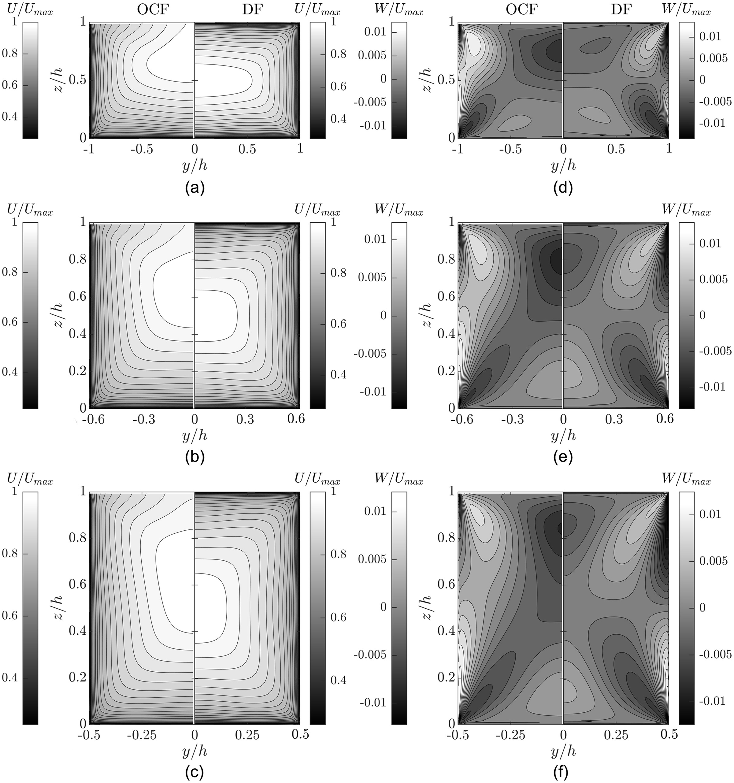

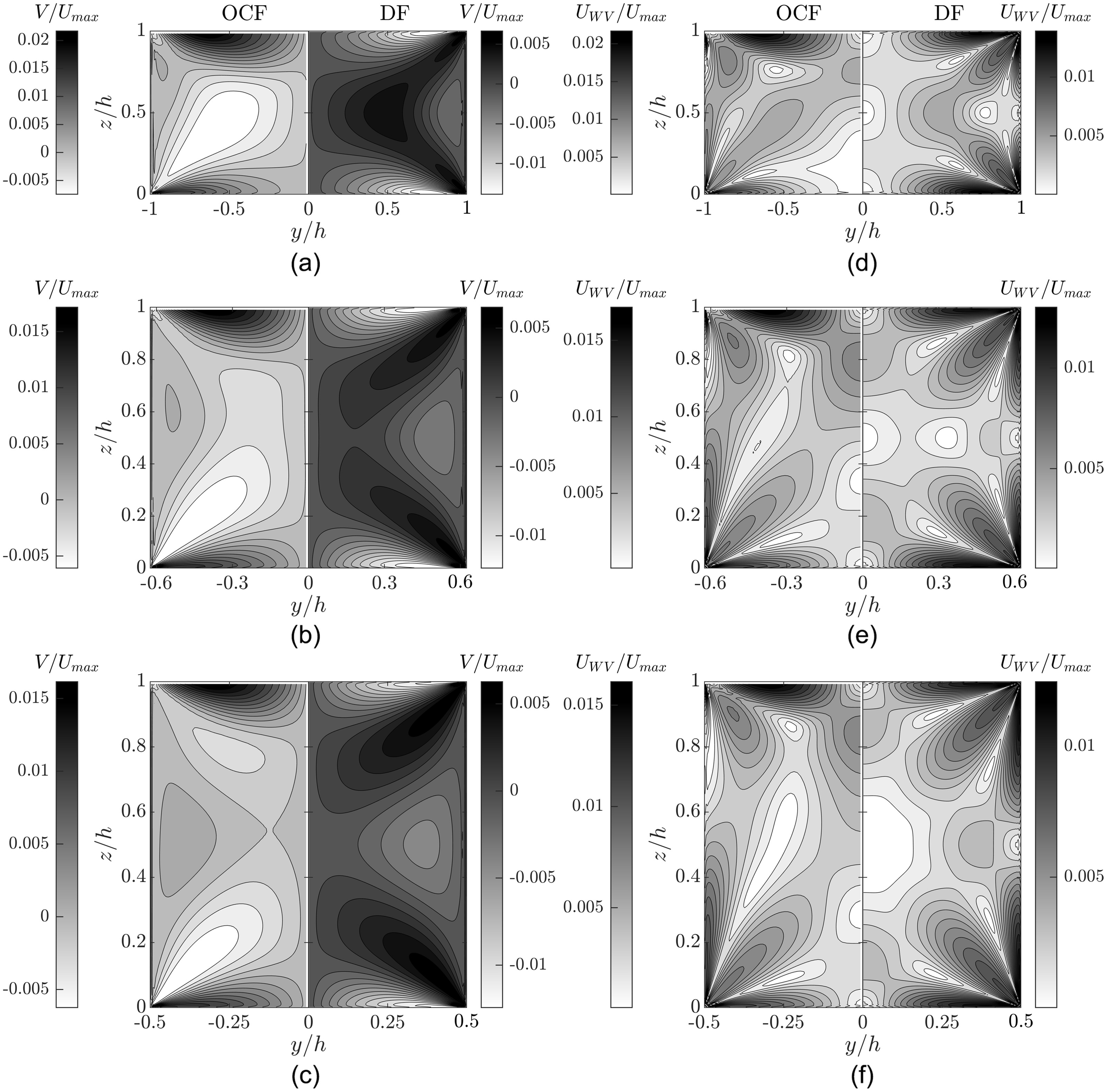
DFs produce 1.0%–2.3% higher values than OCFs (see Table 2). These values are 14.4%–14.9% higher than for OCFs and 15.5%–17.4% higher than for DFs [see also Fig. 4(a)]. Such incremental values and the relative positions of the velocity-dip can be useful to obtain approximate solution for using the discharge and values only. Marginally higher maximum normalized mean vertical velocity for DFs than for OCFs but significantly lower maximum absolute normalized mean lateral velocity and maximum normalized mean resultant secondary velocity (where the mean resultant secondary velocity ) for DFs than for OCFs (see Table 2) signify the stronger free surface vortices in OCFs than weaker corner vortices in DFs. Interestingly, the deviations reduce with a reduction of as the free surface influence reduces. At the mid width, considerably higher deviations between the OCF and DF profiles, especially in the outer flow region , are observed for the vertical velocity as seen from Fig. 4(b). Broadly, the secondary velocity values provided in Table 2 are comparable to previous studies on OCFs (Albayrak and Lemmin 2011; Broglia et al. 2003; Kadia et al. 2022a, c; Naot and Rodi 1982; Nezu and Nakagawa 1986, 1993; Nezu and Rodi 1985; Tominaga et al. 1989) and on DFs (Melling and Whitelaw 1976; Naot and Rodi 1982; Nezu and Nakagawa 1993). However, Nikitin (2021) reported higher (up to 5% of ) in a DNS study conducted for an OCF with .
| Case name | () | a (%) | (%) | (%) | () | () | () | () | (%) | |
|---|---|---|---|---|---|---|---|---|---|---|
| OCF_2 | 2.643 | 1.22 | 1.27 | 2.17 | 2.17 | 0.0928 | 0.0954 | 8.61 | 8.71 | 1.2 |
| OCF_1.25b | 2.654 | 1.23 | 1.22 | 1.72 | 1.72 | 0.0897 | 0.0903 | 8.06 | 8.46 | 5.0 |
| OCF_1 | 2.65 | 1.21 | 1.22 | 1.62 | 1.62 | 0.0886 | 0.0891 | 7.86 | 8.37 | 6.5 |
| DF_2 | 2.669 () | 1.34 () | 1.34 () | 1.39 () | 1.39 () | 0.0979 () | 0.1 () | 9.59 () | 9.05 () | |
| DF_1.25 | 2.692 () | 1.3 () | 1.3 () | 1.24 () | 1.3 () | 0.0944 () | 0.0943 () | 8.91 () | 8.76 () | |
| DF_1 | 2.712 () | 1.25 () | 1.25 () | 1.24 () | 1.25 () | 0.0929 () | 0.0927 () | 8.63 () | 8.63 () | 0.0 |
Note: The percentage values inside the brackets indicate the deviations of the duct flow results from the corresponding open channel flow results.
a
The values indicate the upward maximum and the values indicate the downward maximum.
b
From Kadia et al. (2022a).
The nearly symmetrical contours observed about the bottom corner bisectors for OCFs, especially for lower values, are comparable to the DF results with same bottom corner conditions [see Figs. 3(a–c)]. Additionally, contour patterns in the bottom half depth for OCFs match fairly with the same found for DFs. In the case of DFs, the diagonal components of the corner vortices push the high-momentum fluids and isovels of toward the corners, whereas the inward lateral components of the sidewall corner vortices [up to for for , and for as seen in Figs. 5 and 6(a–c)] and the inward vertical flows of the bottom and top wall corner vortices push the low-momentum fluids and isovels of toward the center of the flow area as found in Figs. 3(a–c) [see also Figs. 3(d–f), 5, and 6(a–c)]. The inward lateral components of the sidewall corner vortices are restricted up to such values (around which a zone of negligible secondary velocity is formed surrounded by corner vortices) due to the outward lateral components of the bottom and the top wall corner vortices [see Figs. 6(a–c)], which dominate the sidewall corner vortices for . The restriction relaxes with a reduction of , which enlarges the sidewall corner vortices in comparison to the bottom and top wall corner vortices. Therefore, the inward bulging of the isovels of is more pronounced for DF_1 than the same observed for higher of 1.25 and 2.0 as found in Figs. 3(a–c). Interestingly, the zone of negligible secondary velocity is also found for OCF with at and as found in Figs. 6(c–d). In OCFs, fully developed intermediate vortices are observed for [comparable to Broglia et al. (2003) and Kadia et al. (2022a)], which are developing for [see Fig. 6(b)] and absent for [see Fig. 6(a)]. The inward lateral components of the developing or the developed intermediate vortices at around 0.5–0.6 [see Figs. 5(b–c)] push the low-momentum fluids inward and result in bulging of the isovels of toward the channel center. In both OCFs and DFs, the reduction of eases the lateral transfer of low-momentum fluids toward the center of the flow area and results in narrowing the area of higher velocity fluids as found in Figs. 3(a–c). Although the bottom wall corner vortices are prominent up to the mid width for DFs, the similar (i.e., the bottom vortices in OCFs) could not reach the mid width for wider channels, especially for the OCF_2 case, as observed from Figs. 3(d–f) and 6(a–c). As a result, the upward bulging of the isovels of away from the bed for the OCF_1 and OCF_1.25 cases is similar to that observed for the DF_1 and DF_1.25 cases, respectively, but differs noticeably for as observed from Figs. 3(a–c). In the case of OCFs, the diagonal components of the bottom vortices and free surface vortices (additionally intermediate vortex components when they exist) toward the bottom corner bisectors bulge the isovels of toward the corners [see Figs. 3(a–c) and 6].

Unlike the lower half flow depth, significant differences between the OCF velocity fields and DF velocity fields are observed in the upper half flow depth due to the differences in top boundary conditions. The no slip top wall in DFs produces steeper velocity gradients and enhanced velocity-dip phenomena compared to those obtained in OCFs with free surface [see Figs. 3(a–c) and 4(a)] although the OCFs produce stronger secondary velocities than DFs as discussed earlier [relate Figs. 3(d–f), 4(b), 5(a–c), and 6 and Table 2]. Unlike in DFs, where the flow conditions are mirrored about the mid depth, in OCFs, the free surface vortices spatially dominate the other vortices as shown in Figs. 6(a–c), especially for higher values. The inward lateral components near the free surface [see Figs. 5(a–c) and 6] and the downward components near the channel center [see Figs. 3(d–f) and 6] of the free surface vortices convey the low-momentum fluids toward the mid width from the sidewalls, which bulges the isovels of toward the center of the flow area and results in velocity dips as found in Figs. 3(a–c). For OCF_2, the outward lateral components of the free surface vortices at transfer the high-momentum fluids toward the sidewalls and push the isovels of outward. Such transfer of fluids relaxes and even opposes with the decrease in (and the development of intermediate vortices) as found in Figs. 3(b and c). In addition, Fig. 6 shows that the inner secondary vortices formed at the mixed corners in OCFs are smaller than the free surface vortices [also reported previously by Grega et al. (1995, 2002), Broglia et al. (2003), Kang and Choi (2006), Nikitin (2021), and Kadia et al. (2022a, 2024)] and as compared to the corner vortices in DFs. However, such small-scale vortices could still alter the isovels of at the top mixed corners as seen in Figs. 3(a–c).
Mean Turbulence Characteristics and Mean Longitudinal Vorticity
The longitudinal, vertical, and lateral turbulence intensities are computed from the converged solutions of the specific Reynolds (normal) stresses as , , and , respectively [Figs. 7 and 8(a–c)]. The shear velocity values at the bed and sidewall were obtained from the log-law (von Kármán 1930; Prandtl 1932) using an integral constant of 5.29 used previously by Nezu and Rodi (1986), Nezu and Nakagawa (1993), Auel et al. (2014), and Demiral et al. (2020) and following Kadia et al. (2022a). The bulging of contour lines is stronger than that of contour lines [comparing Figs. 3(a–c) with Figs. 7(a–c)], which agree well with previous findings (Auel et al. 2014; Melling and Whitelaw 1976; Nezu and Nakagawa 1993). However, the trends are opposite; i.e., the higher values are found toward the no slip boundaries where reduces rapidly and produce steeper velocity gradient in the normal direction while the lower values are obtained toward the center of the flow area and around the velocity dips where reduces mildly and produces flatter gradient. The diagonal flows (combining a pair of corner vortices for DFs and combining bottom vortex, free surface vortex, and or intermediate vortex for OCFs) toward the solid corners push contour lines diagonally. Furthermore, the secondary flows around the mid depth and mid width for the and 1.0 cases bulge the contour lines toward the center of the flow area. In the case of OCF_2 and DF_2, contour lines are pushed away from the solid boundaries around and , respectively, but not up to the mid width due to the restricted growth of the bottom vortices. Additionally, the inner secondary vortices modify contour lines at the mixed corners. Figs. 7(a and b) and 9(a) indicate that contour lines in the central area below the mid depth for and 1.25 are more closely spaced for DFs than those found for OCFs. This is apparently influenced by the steeper found in such zones for DFs than those for OCFs [see Figs. 3(a and b) and 4(a)]. Similar variations are also found for , , and TKE [see Figs. 7(d and e), 8(a and b), and 9(b–d)] for and 1.25. Significantly higher deviations (but similar trends) are observed in the central area above the mid depth for , , and possibly due to the stronger bulging of (steeper ) found in such zone for DFs than the same for OCFs. However, the distributions of and primary specific Reynolds shear stress diverge due to dissimilar top boundaries and their influences. In uniform OCFs, reduces toward the free surface and attains the minimum value near the free surface (Auel et al. 2014; Komori et al. 1982; Nezu and Nakagawa 1986, 1993). Such observed trends are comparable to those reported in uniform supercritical flows by Nezu and Nakagawa (1986, 1993), Auel et al. (2014), and Jing et al. (2019). However, the trends can alter in nonuniform flows (Kironoto and Graf 1995; Song and Chiew 2001), while further deviations are observed in decelerating supercritical flows with higher Froude numbers (Demiral et al. 2020) experiencing surface perturbation and surface undulations as reported by Auel et al. (2014) and discussed by Kadia et al. (2022a), which apparently restrict the damping of . In contrast, increases in the central area above the mid depth for DFs as found in Figs. 7(d–f) and 9(b). However, does not change significantly very close to the bed and top wall due to its damping and redistribution. Interestingly, the distributions of the gap between and (represented by the turbulence anisotropy stress ) observed in the central area for DFs differ insignificantly from the same found for OCFs as seen from Figs. 8(d–f) and 9(f). Besides, the patterns of near the sidewalls for DFs are comparable to those for OCFs, where the maximum values [and the maximum negative turbulence anisotropy shown in Figs. 8(d–f)] are observed for both flow types [Figs. 7(d–f)] due to the comparable damping and redistribution of toward the sidewalls [see Figs. 8(a–c)]. Similarly, the damping and redistribution of toward the bed and top wall or the free surface increases toward such boundaries [see Figs. 7(d–f), 8(a–c), and 9(b and c)]. As a result, the maximum positive turbulence anisotropy values are obtained near such boundaries [Figs. 8(d–f)]. Overall, the distributions of , , and in the bottom half depth of DFs are comparable to the same observed in OCFs, especially for lower values 1.25 and 1.0. In addition, the magnitudes of the turbulence intensities presented in Fig. 9 indicate that the major contributor to is the longitudinal component, followed by lateral and vertical components. However, the maximum and values, where = bed shear velocity at the mid width, obtained near the bed are comparatively lower than the theoretical (Nezu and Nakagawa 1993) and experimental (Auel et al. 2014; Demiral et al. 2020) values, which is a limitation of the used RSM, as also noticed by Cokljat (1993).


The primary specific Reynolds shear stress is obtained from the converged solutions of the Reynolds shear stress component . Figs. 9(e) and 10(a–c) indicate that extrema values are attained close to the no slip walls for both OCFs and DFs, which is attributed to the steeper gradient there. Although the distributions of in the bottom half flow depth are mostly comparable, significant differences are observed above the mid depth. First, the weaker bulging of contour lines above the mixed corner bisectors (i.e., weaker velocity dips and flatter ) for OCFs [see Figs. 3(a–c)] produces more distantly spaced contour lines of negative there than those obtained for DFs. It further generates absolute minimum values around 0.2 for OCFs, which are consistent with previous experimental data (Nezu and Nakagawa 1993; Nezu and Rodi 1985) and numerical results (Broglia et al. 2003; Kadia et al. 2022a, c; Kang and Choi 2006; Shi et al. 1999) but are significantly lower than DFs as seen in Figs. 10(a–c). Second, with a decrease in , the intermediate vortex develops and modifies isovels, and thus, the contour line of around the channel quarters above the mid depth for OCFs is pushed toward the free surface and follows the patterns as in DFs. Such an interesting feature is clearly seen in Figs. 10(b–c) at to and around 0.55 to 0.6 for OCF_1.25, and more clearly for OCF_1 at around and around 0.5 to 0.6 [comparable to the findings of Broglia et al. (2003)]. Lastly, the positive values observed at around 0.95 for OCFs are attributed to the inward lateral components of the small-scale inner secondary vortices, which create there [see Figs. 3(a–c) and 10(a–c)].

The antisymmetric nature of the turbulence anisotropy stress at the solid and mixed corners and its steeper gradients toward the corners are the major contributors to the generation of counterrotating secondary flows at the corners, which are reflected from the vorticity equation provided by Einstein and Li (1958), Demuren and Rodi (1984), Nezu and Nakagawa (1984, 1993), Kang and Choi (2006), and Nikora and Roy (2012). Interestingly, contour lines for DFs are comparable to those for OCFs [Figs. 8(d–f)], especially for and 1.0 and more specifically for the bottom half flow depth. The differences between the free surface and solid top wall effects on the Reynolds stresses produce some dissimilarity in contour lines above the mid depth as seen in Figs. 8(d–f). Such a difference can produce different turbulence anisotropy gradients (toward the corners), which are relevant to the vorticity production. Eventually, the secondary current patterns for DFs obtained from the mean secondary velocity vector plots (Fig. 6) and mean longitudinal vorticity contours [around the mid depth in Figs. 10(d–f)] differ from those for OCFs. It is apparently impacted by the similar influences (on the damping and redistribution of the Reynolds stresses) of the sidewalls and top and bottom walls in DFs, but dissimilar influence of free surface and solid boundaries in OCFs. Furthermore, the spatial domination of the free surface vortices in OCFs produces small-scale inner secondary vortices (smaller than the sidewall corner vortices in DFs) and restricts the development of intermediate vortices at higher [see Figs. 6 and 10(d–f)]. The turbulence anisotropy distribution observed for OCF_2 [Fig. 8(d)] agrees well with previous studies performed for similar (Cokljat 1993; Cokljat and Younis 1995; Shi et al. 1999). In addition, two pairs of counterrotating corner vortices are found in one half of the ducts [see Figs. 10(d–f)], which are antisymmetric about the mid depth, as also visible from Figs. 6(a–c). The sidewall corner vortices swell, and the top and bottom corner vortices shrink with a reduction of . The vorticity plots indicate that the intermediate vortex is a part of the free surface vortex that separates with a decrease in for OCFs. Although a fully developed intermediate vortex is found for OCF_1, a part of the free surface vortex still reaches the bottom solid corner before going up toward the free surface while covering the intermediate vortex. In the lower flow region, the longitudinal vorticity distribution for OCF_1 is comparable to the same for DF_1.
Lateral Distribution of Bed Shear Stress and Vertical Distribution of Wall Shear Stress
Computation of the cross-sectional distribution of the boundary shear stress is crucial for better estimation of sediment transport and safer design of channels from erosion and of SBTs from hydro-abrasion, which can play a significant role in defining the capital and maintenance costs of such designs. The difference in the secondary currents between OCFs and DFs and the influence of on such flow structures impacts the boundary shear stress. The obtained , , laterally averaged bed shear stress , and depth averaged wall shear stress values for OCFs and DFs with a constant bulk velocity are compared in Table 2. Interestingly, higher (between 4.9% and 5.5%), i.e., higher (between 9.8% and 11.4%) values are found for DFs as compared to OCFs. The trend is the same across the entire channel width as reflected from Fig. 11(a) and is related to the higher near wall gradient observed for DFs than OCFs as found at the mid width (as an example) from the slopes of profiles provided in Fig. 4(a). However, the increments of (between 3.1% and 3.9%) are comparatively lower than those observed for . Interestingly, the increments of and decrease marginally (for , from being 11.4% for to 9.8% for and for , from being 3.9% for to 3.1% for ) with an increase in the flow depth or reduction of (i.e., reduction of the free surface contribution as compared to the flow depth). The decrease in reduces both and for OCFs as well as for DFs. However, such reductions are greater for than the same for . Additionally, the reduction of increases the deviation between and for OCFs but decreases the same for DFs as found in Table 2. Eventually, the quantities become equal for a square duct, i.e., both being for the tested conditions. Remarkably, such value is very close to the () and () values obtained for OCF_2. The restricted lateral growth of the bottom vortices undulates distributions for [see Figs. 3(d–f), 4(b), 6, and 11]. However, the distributions become more regular for lower values 1.25 and 1.0 as the bottom vortices reach the mid width. In all cases, the downflows of the bottom vortices toward the sidewall push the isovels of toward the bed and increase , whereas the upward flows toward the mid width for 1.25 and 1.0 and around the channel quarter for bulge the isovels of away from the bed, which reduces . Additionally, the bed shear increases toward the mid width for . The obtained undulations for OCF_2 and DF_1 are comparable to the results reported previously by Nezu and Rodi (1985) and Nezu and Nakagawa (1986, 1993) for similar values. However, those studies compared the OCF results obtained for with the DF results obtained for (although their consideration of = half flow depth, using horizontal symmetry plane, for DF makes ) and observed a significant difference between the profiles as also found in Fig. 11. Such a difference is attributed to the development of bottom vortices whose lateral extends reach up to the mid width for DF_1 but are limited up to the channel quarter for OCF_2 (see Fig. 6). Therefore, the bed shear stress distribution of a square duct cannot be compared to that of an OCF with even though values are close (see Table 2). For and 1.0, the lateral distributions of for OCFs differ insignificantly from those obtained for DFs as seen in Fig. 11(b).

The normalized wall shear stress increases up to but decreases above such and up to the mid depth for DFs (see Fig. 12) due to the outward and inward components of the sidewall corner vortices, respectively, which alter isovels and near wall gradient . In contrast, increases around the mid depth for OCF_2 as the outward flow of the free surface vortices push contour lines toward the sidewall. Such increments relax and values remain roughly constant with the developing (for OCF_1.25) and developed (for OCF_1) intermediate vortices, which push the low-momentum fluids toward the mid width (see Figs. 6 and 12). In addition, the rapid rise in toward the free surface is attributed to the outward bulging of contour lines due to the small-scale inner secondary vortices. Similarly, the inward bulging of contour lines due to such vortices around reduces the near wall and eventually the wall shear. Such influence of the inner secondary vortices was reported previously by Kang and Choi (2006) for a subcritical flow with . However, the Speziale et al. (1991) or SSG RSM used by Kang and Choi (2006) simulated weaker bulging of the contour lines toward the bottom solid corner and, thus, observed lower near the bed as seen in Fig. 12. It is challenging to experimentally determine the impact of inner secondary vortices because of the difficulties in measuring the velocity data close to the boundaries at the mixed corner. Therefore, Nezu and Rodi (1985) could not provide the near free surface undulation of . The vertical distribution of can be useful in the design of sidewall or bank erosion protections.

Potential Scale Effect and Upscaling of the Results
The simulated OCF conditions are comparable to the recent experimental studies on high-speed flows, e.g., Auel et al. (2014, 2017a, b) and Demiral et al. (2020, 2022), and the studied Re and values (see Table 1) satisfy the recommended minimum values of (Boes and Hager 2003) and 0.04 m (Heller 2011), respectively, to limit the scale effects in high-speed flows. Therefore, the results can be scaled up for geometric, kinematic, and dynamic similarities to compare the prototype designs using Froude similitude [see Heller (2011) and Pummer and Schüttrumpf (2018)]. For example, the scale factor for Solis SBT = existing channel width divided by model . Furthermore, Demiral-Yüzügüllü (2021) compared the hydro-abrasion results from the scaled flow, sediment, and invert material conditions with the field observations and observed no or negligible scale effects. In addition, the tested DFs have significantly higher Re than fully turbulent DF cases tested by Pirozzoli et al. (2018) and Nikitin (2021) using DNS, where it was found that the development of the corner vortices and their effect on the flow properties depended on Re when it was comparatively low. The results obtained for the DFs can be scaled up using the geometric scale and Euler number similarity (Aberle et al. 2020). However, further research at project scale shall enlighten the existing knowledge.
Conclusions
The present numerical study compares the mean velocity fields, secondary currents, velocity dips, turbulence properties, and bed and wall shear stress distributions in three supercritical narrow open channel flows (OCFs) of aspect ratios , 1.25, and 2.0, comparable to sediment bypass tunnel flow conditions, with those in three duct flows (DFs). Steady state uniform flow simulations were performed in OpenFOAM using a modified Launder, Reece, and Rodi Reynolds stress model, which was validated previously for supercritical flows by Kadia et al. (2022a). The used numerical approach is fast and computationally more economical than transient options but limits to uniform flow conditions. Overall, the three-dimensional turbulent flow characteristics of narrow OCFs differ from the same found in narrow square or rectangular DFs, especially above the mid depth, due to the difference between the free surface and top wall boundaries, whose damping and redistribution effects on the turbulence intensities are dissimilar. The major conclusions drawn from the comparison between OCFs and DFs are as follows:
•
Top no slip wall in DFs produces steeper velocity gradient and enhanced velocity-dip phenomenon compared to those in OCFs even though the free surface in OCFs generates maximum secondary velocity values that are greater than those are in DFs.
•
Unlike DFs, in which the turbulence intensity components, turbulent kinetic energy, and turbulence anisotropy stress all increase sharply in the central flow area above the mid depth due to the solid top wall, the free surface in OCFs produces comparatively lesser increments in the longitudinal and lateral turbulence intensities and turbulent kinetic energy above the velocity dips, and even sharp reduction in the vertical turbulence intensity there. However, the difference in the turbulence anisotropy stress is less significant. The observed damping of the vertical turbulence intensity toward the free surface agrees well with the uniform supercritical flow experiments reported in the literature.
•
In DFs, two antisymmetric pairs of counterrotating vortices are observed in each half width, and a reduction of enlarges the sidewall adjacent corner vortices in comparison with the remaining ones. Although decreasing for OCFs swells the bottom vortices, narrows and deepens the free surface vortices, and develops the intermediate vortices, it imposes an insignificant impact on the inner secondary vortices. These alternations of secondary currents are interrelated to the redistributions of longitudinal velocity and turbulence parameters among the flow zones toward the corners, boundaries, and central area. Interestingly, the intermediate vortices in the square channel impose similar effects on the flow properties such as the sidewall corner vortices in DFs.
•
DFs produce higher and as compared to OCFs. However, the percentage increase of is greater than that of . These percentage values are impacted insignificantly by because the increasing produces greater raise of for both OCFs and DFs than the respective raise of . The bottom vortices undulate the bed shear stress distributions whereas the sidewall corner vortices (in DFs) or the intermediate vortices and inner secondary vortices (in OCFs) undulate the wall shear stress distributions, which are influenced by . These observations are of utmost importance for the hydraulic design of tunnels and bed rock channels regarding sediment transport and hydro-abrasion processes, i.e., patterns and depths.
•
The flow characteristics in the bottom half depth of OCFs are comparable with those of DFs, especially for the square cross sections with .
•
The turbulent flow characteristics in a square duct are not comparable with those in an OCF with .
•
Overall, the used model is suitable to compute the turbulent flow characteristics and boundary shear stress in high-speed uniform and quasi-uniform narrow OCFs (when the free surface undulations are limited) and narrow DFs.
The present findings provide a comprehensive characterization of narrow OCFs and DFs useful in designing the channels and tunnels conveying high-speed sediment laden flows and will underpin follow up studies. In particular, the separation of intermediate vortex from the free surface vortex for narrower OCFs demands further numerical (LES and DNS) and experimental investigations. Furthermore, the model can be scaled up for project flow conditions based on the Froude similitude since no scale effect is expected for the tested and high Re. Lastly, the updated LRR RSM in OpenFOAM can further be modified by the users for 3D grid arrangements, irregular cross sections, and parallel processing.
Notation
The following symbols are used in this paper:
- aspect ratio;
- width of open channel or duct (m);
- hydraulic diameter (m);
- Froude number;
- flow depth (m);
- turbulent kinetic energy ();
- production of turbulent kinetic energy ();
- pressure ( in general, but in simpleFoam);
- Reynolds number;
- turbulence anisotropy stress ();
- specific Reynolds stress tensor ();
- , , and
- mean longitudinal, lateral, and vertical velocities ();
- mean resultant secondary velocity ();
- bulk velocity ();
- laterally averaged bed shear velocity ();
- , , and
- longitudinal, lateral, and vertical turbulence intensities ();
- , , and
- longitudinal, lateral, and vertical velocity fluctuations ();
- bed shear velocity at the mid width ();
- primary specific Reynolds shear stress ();
- lateral distance from the mid width (m);
- vertical distance from the bed (m);
- dissipation rate of turbulent kinetic energy ();
- and
- kinematic viscosity and eddy-viscosity ();
- and
- bed shear stress and laterally averaged bed shear stress ();
- and
- wall shear stress and depth averaged wall shear stress ();
- pressure-strain tensor (); and
- mean longitudinal vorticity ().
Data Availability Statement
Acknowledgments
This study is funded by NTNU (project number 81772024) and supported by HydroCen (project number 90148311).
References
Aberle, J., P. Y. Henry, F. Kleischmann, C. U. Navaratnam, M. Vold, R. Eikenberg, and N. R. B. Olsen. 2020. “Experimental and numerical determination of the head loss of a pressure driven flow through an unlined rock-blasted tunnel.” Water 12 (12): 3492. https://doi.org/10.3390/w12123492.
Albayrak, I., and U. Lemmin. 2011. “Secondary currents and corresponding surface velocity patterns in a turbulent open-channel flow over a rough bed.” J. Hydraul. Eng. 137 (11): 1318–1334. https://doi.org/10.1061/(ASCE)HY.1943-7900.0000438.
Alfonsi, G. 2009. “Reynolds-averaged Navier-Stokes equations for turbulence modeling.” Appl. Mech. Rev. 62 (4): 040802. https://doi.org/10.1115/1.3124648.
Almeland, S. K., T. Mukha, and R. E. Bensow. 2021. “An improved air entrainment model for stepped spillways.” Appl. Math. Modell. 100 (Dec): 170–191. https://doi.org/10.1016/j.apm.2021.07.016.
Auel, C., I. Albayrak, and R. M. Boes. 2014. “Turbulence characteristics in supercritical open channel flows: Effects of Froude number and aspect ratio.” J. Hydraul. Eng. 140 (4): 04014004. https://doi.org/10.1061/(ASCE)HY.1943-7900.0000841.
Auel, C., I. Albayrak, T. Sumi, and R. M. Boes. 2017a. “Sediment transport in high-speed flows over a fixed bed: 1. Particle dynamics.” Earth Surf. Processes Landforms 42 (9): 1365–1383. https://doi.org/10.1002/esp.4128.
Auel, C., I. Albayrak, T. Sumi, and R. M. Boes. 2017b. “Sediment transport in high-speed flows over a fixed bed: 2. Particle impacts and abrasion prediction.” Earth Surf. Processes Landforms 42 (9): 1384–1396. https://doi.org/10.1002/esp.4132.
Boes, R. M., and W. H. Hager. 2003. “Two-phase flow characteristics of stepped spillways.” J. Hydraul. Eng. 129 (9): 661–670. https://doi.org/10.1061/(ASCE)0733-9429(2003)129:9(661).
Broglia, R., A. Pascarelli, and U. Piomelli. 2003. “Large-eddy simulations of ducts with a free surface.” J. Fluid Mech. 484 (Jun): 223–253. https://doi.org/10.1017/S0022112003004257.
Caretto, L. S., A. D. Gosman, S. V. Patankar, and D. B. Spalding. 1973. “Two calculation procedures for steady, three-dimensional flows with recirculation.” In Proc., 3rd Int. Conf. on Numerical Methods in Fluid Mechanics, 60–68. Berlin: Springer. https://doi.org/10.1007/BFB0112677.
Cokljat, D. 1993. “Turbulence models for non-circular ducts and channels.” Doctoral thesis, Dept. of Civil Engineering, Univ. of London.
Cokljat, D., and B. A. Younis. 1995. “Second-order closure study of open-channel flows.” J. Hydraul. Eng. 121 (2): 94–107. https://doi.org/10.1061/(ASCE)0733-9429(1995)121:2(94).
Daly, B. J., and F. H. Harlow. 1970. “Transport equations in turbulence.” Phys. Fluids 13 (11): 2634–2649. https://doi.org/10.1063/1.1692845.
Demiral, D., I. Albayrak, J. M. Turowski, and R. M. Boes. 2022. “Particle saltation trajectories in supercritical open channel flows: Roughness effect.” Earth Surf. Processes Landforms 47 (15): 3588–3610. https://doi.org/10.1002/esp.5475.
Demiral, D., R. M. Boes, and I. Albayrak. 2020. “Effects of secondary currents on turbulence characteristics of supercritical open channel flows at low aspect ratios.” Water 12 (11): 3233. https://doi.org/10.3390/w12113233.
Demiral-Yüzügüllü, D. 2021. “Hydro-abrasion processes and modelling at hydraulic structures and steep bedrock rivers.” Ph.D. thesis, Laboratory of Hydraulics, Hydrology and Glaciology, ETH Zürich.
Demuren, A. O., and W. Rodi. 1984. “Calculation of turbulence-driven secondary motion in non-circular ducts.” J. Fluid Mech. 140 (Mar): 189–222. https://doi.org/10.1017/S0022112084000574.
Dey, S. 2014. “Fluvial hydrodynamics: Hydrodynamic and sediment transport phenomena.” In GeoPlanet: Earth and planetary sciences. Berlin: Springer. https://doi.org/10.1007/978-3-642-19062-9.
Einstein, H. A., and H. Li. 1958. “Secondary currents in straight channels.” Eos, Trans. Am. Geophys. Union 39 (6): 1085–1088. https://doi.org/10.1029/TR039i006p01085.
Gessner, F. B. 1973. “The origin of secondary flow in turbulent flow along a corner.” J. Fluid Mech. 58 (1): 1–25. https://doi.org/10.1017/S0022112073002090.
Gibson, M. M., and B. E. Launder. 1978. “Ground effects on pressure fluctuations in the atmospheric boundary layer.” J. Fluid Mech. 86 (3): 491–511. https://doi.org/10.1017/S0022112078001251.
Gibson, M. M., and W. Rodi. 1989. “Simulation of free surface effects on turbulence with a Reynolds stress model.” J. Hydraul. Res. 27 (2): 233–244. https://doi.org/10.1080/00221688909499183.
Greenshields, C. 2022. OpenFOAM v10 user guide. London: OpenFOAM Foundation.
Greenshields, C., and H. Weller. 2022. Notes on computational fluid dynamics: General principles. Reading, UK: CFD Direct.
Grega, L. M., T. Y. Hsu, and T. Wei. 2002. “Vorticity transport in a corner formed by a solid wall and a free surface.” J. Fluid Mech. 465 (Aug): 331–352. https://doi.org/10.1017/S0022112002001088.
Grega, L. M., T. Wei, R. I. Leighton, and J. C. Neves. 1995. “Turbulent mixed-boundary flow in a corner formed by a solid wall and a free surface.” J. Fluid Mech. 294 (Jul): 17–46. https://doi.org/10.1017/S0022112095002795.
Guo, J. 2014. “Modified log-wake-law for smooth rectangular open channel flow.” J. Hydraul. Res. 52 (1): 121–128. https://doi.org/10.1080/00221686.2013.818584.
Hanjalić, K., and B. E. Launder. 1972. “A Reynolds stress model of turbulence and its application to thin shear flows.” J. Fluid Mech. 52 (4): 609–638. https://doi.org/10.1017/S002211207200268X.
Heller, V. 2011. “Scale effects in physical hydraulic engineering models.” J. Hydraul. Res. 49 (3): 293–306. https://doi.org/10.1080/00221686.2011.578914.
Jing, S., W. Yang, and Y. Chen. 2019. “Smooth open channel with increasing aspect ratio: Influence on secondary flow.” Water 11 (9): 1872. https://doi.org/10.3390/w11091872.
Kadia, S., L. Lia, I. Albayrak, and E. Pummer. 2024. “The effect of cross-sectional geometry on the high-speed narrow open channel flows: An updated Reynolds stress model study.” Comput. Fluids 271 (Mar): 106184. https://doi.org/10.1016/j.compfluid.2024.106184.
Kadia, S., E. Pummer, and N. Rüther. 2021. “CFD simulation of supercritical flow in narrow channels including sediment bypass tunnels.” In Proc., 8th Int. Junior Researcher and Engineer Workshop on Hydraulic Structures, 7. Logan, UT: Utah State Univ. https://doi.org/10.26077/e5fd-df7a.
Kadia, S., N. Rüther, I. Albayrak, and E. Pummer. 2022a. “Reynolds stress modeling of supercritical narrow channel flows using OpenFOAM: Secondary currents and turbulent flow characteristics.” Phys. Fluids 34 (12): 125116. https://doi.org/10.1063/5.0124076.
Kadia, S., N. Rüther, I. Albayrak, and E. Pummer. 2022b. Updated LRR Reynolds stress model in OpenFOAM: The modified code files (v1.0). Geneva: Zenodo. https://doi.org/10.5281/zenodo.7313194.
Kadia, S., N. Rüther, and E. Pummer. 2022c. “Reynolds stress modelling of supercritical flow in a narrow channel.” In Proc., 9th Int. Symp. on Hydraulic Structures, 58. Roorkee, India: Utah State Univ. https://doi.org/10.26077/5e0b-783d.
Kang, H., and S. U. Choi. 2006. “Reynolds stress modelling of rectangular open-channel flow.” Int. J. Numer. Methods Fluids 51 (11): 1319–1334. https://doi.org/10.1002/fld.1157.
Kim, S. E. 2001. “Unstructured mesh based Reynolds stress transport modeling of complex turbulent shear flows.” In Proc., 39th Aerospace Sciences Meeting and Exhibit, 728. Reno, NV: AIAA. https://doi.org/10.2514/6.2001-728.
Kironoto, B. A., and W. H. Graf. 1995. “Turbulence characteristics in rough non-uniform open-channel flow.” Proc. Inst. Civ. Eng. Water Marit. Energy 112 (4): 336–348. https://doi.org/10.1680/iwtme.1995.28114.
Komori, S., H. Ueda, F. Ogino, and T. Mizushina. 1982. “Turbulence structure and transport mechanism at the free surface in an open channel flow.” Int. J. Heat Mass Transfer 25 (4): 513–521. https://doi.org/10.1016/0017-9310(82)90054-0.
Launder, B. E., G. J. Reece, and W. Rodi. 1975. “Progress in the development of a Reynolds-stress turbulence closure.” J. Fluid Mech. 68 (3): 537–566. https://doi.org/10.1017/S0022112075001814.
Melling, A., and J. H. Whitelaw. 1976. “Turbulent flow in a rectangular duct.” J. Fluid Mech. 78 (2): 289–315. https://doi.org/10.1017/S0022112076002450.
Müller-Hagmann, M. 2018. “Hydroabrasion by high-speed sediment-laden flows in sediment bypass tunnels.” Ph.D. thesis, Laboratory of Hydraulics, Hydrology and Glaciology, Swiss Federal Institute of Technology in Zürich. https://doi.org/10.3929/ethz-b-000273498.
Naot, D., and W. Rodi. 1982. “Calculation of secondary currents in channel flow.” J. Hydraul. Div. 108 (8): 948–968. https://doi.org/10.1061/JYCEAJ.0005897.
Nezu, I., and H. Nakagawa. 1984. “Cellular secondary currents in straight conduit.” J. Hydraul. Eng. 110 (2): 173–193. https://doi.org/10.1061/(ASCE)0733-9429(1984)110:2(173).
Nezu, I., and H. Nakagawa. 1986. “Investigation on three-dimensional turbulent structure in uniform open-channel and closed duct flows.” [In Japanese.] Doboku Gakkai Ronbunshu 1986 (369): 89–98. https://doi.org/10.2208/jscej.1986.369_89.
Nezu, I., and H. Nakagawa. 1993. Turbulence in Open Channel Flows (IAHR Monographs). Rotterdam, Netherlands: A. A. Balkema.
Nezu, I., and W. Rodi. 1985. “Experimental study on secondary currents in open channel flows.” In Vol. 2 of Proc., 21st IAHR Congress, 115–119. Melbourne, VIC, Australia: Institution of Engineers.
Nezu, I., and W. Rodi. 1986. “Open-channel flow measurements with a laser Doppler anemometer.” J. Hydraul. Eng. 112 (5): 335–355. https://doi.org/10.1061/(ASCE)0733-9429(1986)112:5(335).
Nikitin, N. 2021. “Turbulent secondary flows in channels with no-slip and shear-free boundaries.” J. Fluid Mech. 917 (Jun): A24. https://doi.org/10.1017/jfm.2021.306.
Nikora, V., and A. G. Roy. 2012. “Secondary flows in rivers: Theoretical framework, recent advances, and current challenges.” In Gravel-bed rivers: Processes, tools, environments, edited by M. Church, P. M. Biron, and A. G. Roy, 3–22. Chichester, UK: Wiley. https://doi.org/10.1002/9781119952497.ch1.
Nikuradse, J. 1926. “Turbulente strömung im innern des rechteckigen offenen kanals.” [In German.] Forschungsarbeiten 281: 36–44.
OpenFOAM Foundation. 2022. “OpenFOAM dev: C++ source code guide.” Accessed June 24, 2022. https://cpp.openfoam.org/dev/.
Pirozzoli, S., D. Modesti, P. Orlandi, and F. Grasso. 2018. “Turbulence and secondary motions in square duct flow.” J. Fluid Mech. 840 (Apr): 631–655. https://doi.org/10.1017/jfm.2018.66.
Prandtl, L. 1932. “Zur turbulenten Strömung in Röhren und längs Platten [On turbulent flows in ducts and along plates].” In Ergebnisse der Aerodynamischen Versuchsanstalt zu Göttingen, 18–29. München, Germany: Oldenbourg.
Prandtl, L. 1952. Essentials of fluid dynamics. London: Blackie and Son.
Pummer, E., and H. Schüttrumpf. 2018. “Reflection phenomena in underground pumped storage reservoirs.” Water 10 (4): 504. https://doi.org/10.3390/w10040504.
Reece, G. J. 1977. “A generalized Reynolds-stress model of turbulence.” Doctoral thesis, Faculty of Engineering, Univ. of London.
Rodi, W. 1993. Turbulence models and their application in hydraulics: A state-of-the-art review (IAHR Monographs). Rotterdam, Netherlands: A. A. Balkema.
Rotta, J. 1951. “Statistische Theorie nichthomogener Turbulenz.” [In German.] Zeitschrift für Physik 129 (6): 547–572. https://doi.org/10.1007/BF01330059.
Shi, J., T. G. Thomas, and J. J. R. Williams. 1999. “Large-eddy simulation of flow in a rectangular open channel.” J. Hydraul. Res. 37 (3): 345–361. https://doi.org/10.1080/00221686.1999.9628252.
Shir, C. C. 1973. “A preliminary numerical study of atmospheric turbulent flows in the idealized planetary boundary layer.” J. Atmos. Sci. 30 (7): 1327–1339. https://doi.org/10.1175/1520-0469(1973)030%3C1327:APNSOA%3E2.0.CO;2.
Song, T., and Y. M. Chiew. 2001. “Turbulence measurement in nonuniform open-channel flow using acoustic Doppler velocimeter (ADV).” J. Eng. Mech. 127 (3): 219–232. https://doi.org/10.1061/(ASCE)0733-9399(2001)127:3(219).
Speziale, C. G., S. Sarkar, and T. B. Gatski. 1991. “Modelling the pressure-strain correlation of turbulence : An invariant dynamical systems approach.” J. Fluid Mech. 227 (Jun): 245–272. https://doi.org/10.1017/S0022112091000101.
Talebpour, M. 2016. “Numerical investigation of turbulent-driven secondary flow.” M.S. thesis, Dept. of Civil and Environmental Engineering, Pennsylvania State Univ.
Talebpour, M., and X. Liu. 2019. “Numerical investigation on the suitability of a fourth-order nonlinear k- model for secondary current of second type in open-channels.” J. Hydraul. Res. 57 (1): 1–12. https://doi.org/10.1080/00221686.2018.1444676.
Thomson, J. 1879. “On the flow of water in uniform régime in rivers and other open channels.” Proc. R. Soc. London 28 (190–195): 113–127. https://doi.org/10.1098/rspl.1878.0100.
Tominaga, A., I. Nezu, K. Ezaki, and H. Nakagawa. 1989. “Three-dimensional turbulent structure in straight open channel flows.” J. Hydraul. Res. 27 (1): 149–173. https://doi.org/10.1080/00221688909499249.
von Kármán, T. 1930. “Mechanische Ähnlichkeit und Turbulenz [Mechanical similarity and turbulence].” [In German.] Nachr. Ges. Wiss. Göttingen Mathematisch-Physische Kl. 5: 58–76.
Wilcox, D. C. 2006. Turbulence modelling for CFD. La Canada, CA: DCW Industries.
Yang, S.-Q., S.-K. Tan, and S.-Y. Lim. 2004. “Velocity distribution and dip-phenomenon in smooth uniform open channel flows.” J. Hydraul. Eng. 130 (12): 1179–1186. https://doi.org/10.1061/(ASCE)0733-9429(2004)130:12(1179).
Information & Authors
Information
Published In

Journal of Hydraulic Engineering
Volume 150 • Issue 4 • July 2024
Copyright
This work is made available under the terms of the Creative Commons Attribution 4.0 International license, https://creativecommons.org/licenses/by/4.0/.
History
Received: Jul 3, 2023
Accepted: Jan 23, 2024
Published online: Apr 24, 2024
Published in print: Jul 1, 2024
Discussion open until: Sep 24, 2024
Authors
Metrics & Citations
Metrics
Citations
Download citation
If you have the appropriate software installed, you can download article citation data to the citation manager of your choice. Simply select your manager software from the list below and click Download.