Abstract
A new formulation of the Preissmann Slot for modeling surcharged (pressurized) one-dimensional (1D) pipe flow is presented. The Dynamic Preissmann Slot (DPS) is derived in a nondimensional form where the slot is treated as transient storage, which is a function of slot cross-sectional area rather than width. The use of transient storage area removes the traditional conceptualization of the slot as a simple rectangular shape of fixed width. The transient storage area and its shape evolve dynamically with the flow. A nondimensional smoothing approach, using a newly defined Preissmann Number, is developed to address issues of instabilities and shocks that have been problems for prior Preissmann Slot models. The new model is tested using a Saint-Venant equation finite-volume solver that has been written as an extension of the Storm Water Management Model (SWMM). Comparison of model results to laboratory data from the literature show that the new approach captures mixed-flow dynamics in transitions from unpressurized to pressurized flow and back again.
Introduction
A consequence of aging stormwater infrastructure is that pipes designed for free-surface flow may be more frequently forced into surcharged (pressurized) flow. As such, numerical methods that effectively handle mixed-flow transitions between free-surface and pressurized flow are critical to efficient numerical simulation of stormwater systems. The Preissmann Slot is a long-standing computational approach for simulating one-dimensional (1D), pressurized, closed-conduit flow with the Saint-Venant equations (SVE) of open-channel flow (Cunge and Wegner 1964). Two key problems of the Preissmann Slot are (1) the need to a priori specify a slot width in each section of pipe, which affects algorithm performance and is difficult to set consistently over widely-varying pipe sizes, and (2) the appearance of shocks, oscillations, and numerical instabilities at the interface between surcharged and free-surface pipe sections in a simulation. The oscillations and instabilities caused by mixed-flow shocks result in degraded performance of a numerical solver. For the widely-used US EPA Storm Water Management Model (SWMM), the result is typically slow convergence and poor mass conservation.
In this paper, we show that the underlying ideas of the Preissmann Slot approach can be used without a user-specified slot width. Indeed, the concept of the slot width can be dispensed with entirely except as a heuristic for understanding transient storage. The new approach is called a Dynamic Preissmann Slot (DPS) algorithm. The behavior of the DPS algorithm primarily depends on user-specified global target pressure celerity, whose value is related to the desired representation of acoustic wave speeds, the model time step, and numerical stability constraints—quantities that are easier to identify and comprehend than the behavior of the slot width. A key advantage is that the slot is enforced consistently and smoothly across a simulation domain through a surcharge shock parameter (controlling the shock magnitude at a mixed-flow transition) and a decay time scale (controlling the surcharge celerity rate of change). By dynamically adjusting the slot across the moving boundaries between free-surface and pressurized zones, the new approach limits the development of shocks and numerical instabilities that have plagued users of the traditional Preissmann Slot.
In developing the new DPS approach we identify a nondimensional number—which we propose to call the Preissmann Number that is similar to an inverse Mach Number but is more meaningful for surcharged pipe systems. We show that ensuring a smoothly varying Preissmann Number, , is a non-dimensional approach to providing a smoothly varying celerity in a surcharged conduit.
The Background section provides our motivation with a discussion of the Preissmann Slot and other forms of pressurized flow modeling in closed conduits. In the Methodology section, the new DPS algorithm is derived along with its numerical implementation. In the Results section, the new approach is tested and validated against laboratory experiments of Trajkovic et al. (1999) and Vasconcelos et al. (2006). Implications of the DPS algorithm and the need for further study are considered in the Discussion section. The key findings are summarized in the Conclusion.
Background
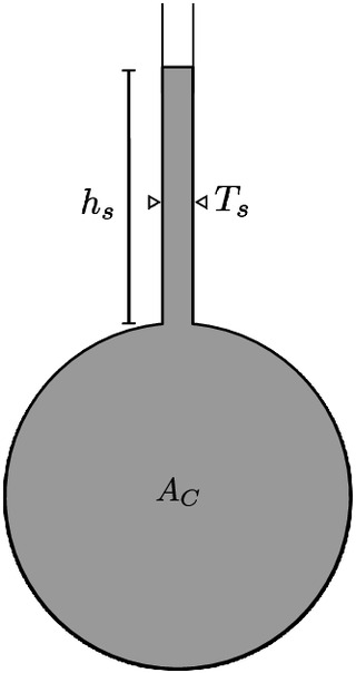
The Preissmann Slot was first demonstrated for simulating surges in a dam penstock by Cunge and Wegner (1964) based on an idea attributed to Preissmann and Cunge (1961). With this innovation, a closed conduit has an imaginary, infinitely-high, narrow, rectangular slot attached at the top of the closed conduit (Fig. 1). The height of water in the slot () represents the surcharge pressure. The goal of the Preissmann Slot is to allow the SVE for free-surface flow to be used in place of weakly-compressible equations or the rigid-column approximation for surcharged flow in a closed conduit. In effect, this is a transient storage model similar to the Two Component Pressure Approach (TPA) and Artificial Compressibility (AC) methods (Vasconcelos et al. 2006; Hodges 2020; Hodges et al. 2022). In SVE implementations of the Preissmann Slot, the slot volume must small compared to the conduit volume and the flow in the slot is treated as frictionless. Although the volume of water in the slot is a representation of transient storage, the Preissmann Slot has not been used to physically parameterize the conduit expansion or fluid compression that causes transient storage.
The key characteristic of the Preissmann Slot is that the simulated pressure celerity () depends upon gravity, the cross-sectional area of the conduit (), and the selected slot width () aswhich was first presented by Cunge and Wegner (1964). The small volume of the slot and neglect of friction within the slot implies its impact on the flow dynamics in the underlying conduit is mainly through the surcharge pressure head. However, the selection of the slot width sets , the speed of a pressure pulse through the surcharged conduit, which can have significant consequences in the modeled results—particularly at the mixed-flow boundary where a celerity shock occurs at the transition between the gravity wave of the free-surface flow and higher-celerity pressurized flow. Further background on celerity shocks is provided in Sharior et al. (2023).
(1)
In Cunge and Wegner (1964), the slot width was a priori selected such that the celerity in the slot matched the expected acoustic celerity () of the pressurized flow. Vasconcelos and Wright (2004) demonstrated that slot size has a significant impact on modeled bore arrival timing, with the bore arriving quicker as the slot size was reduced. Malekpour and Karney (2015) argued that is needed where local system design depends on correctly estimating the filling velocity of a bore propagating into a section of unpressurized conduit. Indeed, in any simulation where short transient timescales are of foremost interest, e.g., pressure pulses causing stormwater geysers (Guo and Song 1990; Zhou et al. 2002), arguably the slot width should be selected to match the acoustic celerity. Unfortunately, precisely evaluating under dynamically-changing conditions is a nontrivial task as depends on the gas fraction in air/water mixtures as well as conduit geometry, materials, and construction techniques (Wylie and Streeter 1983). Furthermore, is indirectly a function of the pressure itself (through conduit expansion and fluid compressibility), whereas is strictly a function of the conduit and slot geometry. Thus, the Preissmann Slot is an approximate model of weak compressibility effects, but does not lend itself to detailed study of the underlying compressibility dynamics as it does not include the equations for the relevant factors.
Nevertheless, despite the ad hoc nature of specifying the Preissmann Slot width and its limitations, over the past 60 years the method has proven well-suited for large-scale modeling of piping systems with episodic mixed flow conditions, i.e., where the system is mostly free-surface flow and a relatively small portion (in time and/or space) of the system has pressurized flow. Such conditions are common in stormwater drainage systems where the precise representation of transient pulses are not (usually) a driving concern. The key advantage of the Preissmann Slot for the model designer is that one set of governing equations (the SVE) are used for both free-surface and pressurized flow sections. Using a single set of dynamic equations across the entire system generally leads to a simpler and more robust numerical model. In contrast, models suited to full-conduit hydraulic transient analyses (Wylie and Streeter 1983; Leon et al. 2008) are typically ill-suited for free-surface flow, which means modeling a mixed-flow system requires two solvers that must trade-off with the time/space locations of surcharging (León et al. 2010; Rokhzadi and Fuamba 2022). To address this issue, transient storage models designed specifically for mixed-flow conditions have been proposed (e.g., Song et al. 1983; Cardle and Song 1988; Vasconcelos and Wright 2007; Hodges 2020). As yet, these computationally intense models have not proven practical for large stormwater networks where the majority of the system is free-surface flow and pressurization events are episodic in space and time.
The Preissmann Slot has been criticized for numerical oscillations and stability issues that occur when the flow transitions across the mixed-flow boundary from free-surface to pressurized flow (Vasconcelos et al. 2009; León et al. 2009; Malekpour and Karney 2015). The common remedies in literature are (1) setting of Eq. (1) such that , (2) applying oscillation suppression filters, and (3) introducing slots that are wider at the conduit crown and smoothly narrow with increasing elevation (Sjöberg 1982; Capart et al. 1997; León et al. 2009; Vasconcelos et al. 2009; Malekpour and Karney 2015). The third approach, a tapering slot, requires Eq. (1) be rewritten in terms of the slot area, , as detailed in Sharior et al. (2023), which results in
(2)
Unlike the fixed slot width of Eq. (1) that results in a fixed value for , the slot with a tapering width in Eq. (2) results in a time-space varying that depends on the accumulated slot area () at a given surcharge height (). While such functionality does not necessarily represent real-world behavior, it serves to ensure that the transition from free-surface to pressurized flow (at low surcharge) has a smaller and hence is less likely to have oscillatory behavior. This idea of a tapering slot is the foundation of the present work. The first to propose this appears to be Sjöberg (1982), but their model required additional numerical dissipation to damp oscillations. A more successful approach was that of León et al. (2009) who prescribed a slot that tapered from 95% of the pipe diameter to the desired of the slot at 50% of the pipe diameter above the crown. Their tapering approach provided a successful model but their definition was inherently ad hoc, static, and dimensional, which inspired the present work to create a non-dimensional dynamic approach where control of the slot is inherently based on fluid behavior rather than conduit geometry.
The slot width () in many of the Preissmann Slot applications in the literature is not predicated on representing . Most modeling focuses on larger timescales where slower pressure celerity will not have a significant impact. The is often decided based on practical considerations associated with (1) the computational effort implied by the small model time-step required for the celerity , and (2) suppressing oscillations and/or instabilities associated with celerity shocks. There have been a wide range of conditions paired with different numerical schemes in literature. For example, Garcia-Navarro et al. (1994) used a fixed for a conduit of diameter (), which reduces from to . The Preissmann Slot in the SWMM model—reintroduced in Version 5, Build 5.1.013, (USEPA 2022)—uses , which results in for in m; i.e., the modeled is less than 5% of typical acoustic celerities for . Setting a larger value of is a common approach (Capart et al. 1997; Ji 1998; Trajkovic et al. 1999), which results in for in m; i.e., the modeled is less than 1.5% of typical acoustic celerities for . Other transient-storage models have used similarly reduced celerities. For example, the TPA model of Vasconcelos et al. (2006) used a to minimize the numerical oscillation due to shocks. The hybrid numerical scheme of An et al. (2018) used ; they noted that larger caused spurious oscillations. There are a few studies that used however, most reported numerical oscillation and stability issues (Vasconcelos et al. 2009; León et al. 2009; Sanders and Bradford 2010; Kerger et al. 2011; Malekpour and Karney 2015; Lieb et al. 2016). Our Discussion section provides further insight on oscillations relative to the present work.
In the methodology developed in the following, we show that the traditional formulation of the Preissmann Slot—where the slot width is the principal ad hoc control—can be inverted to make pressure celerity the controlling parameter. This idea leads to an approach that is effectively a dynamic Preissmann Slot—a slot whose width changes in both time and space to create smooth transitions across mixed-flow boundaries. This idea has its genesis in the smoothing approaches investigated by Capart et al. (1997), León et al. (2009), Vasconcelos et al. (2009), and Malekpour and Karney (2015). The key innovation in the present work is through providing dynamic control of the shape and cross-section of the Preissmann Slot to smooth celerity gradients, thereby reducing shocks and yet allowing or to the modeler’s desired celerity.
Methodology
Overview
To address the outstanding difficulties of the Preissmann Slot we propose a reformulated relationship between the surcharge pressure head increment (i.e., the traditional slot height, ) and the transient storage cross-sectional area (, traditionally the product ). To do this, we introduce the concept of a pressure celerity target, , that is a modeler’s desired global pressure celerity for the surcharged system, i.e., the model’s replacement for the true acoustic pressure celerity, . For true transient analysis, can be used, but for many systems—particularly those with both free-surface and surcharged sections—values of will be desired to allow stable and accurate solutions at larger time steps. Furthermore, we introduce the idea that a conduit may have spatial and temporal distributions such that is allowed to ensure smoothly-varying pressure celerity throughout the system during time-varying surcharging, across transitions in pipe size, and where free-surface flow meets surcharged flow. We believe this generalized Dynamic Preissmann Slot (DPS) will solve some of the long-standing stability issues in prior approaches.
The DPS model is implemented within the new SWMM5+ hydraulic solver (Hodges et al. 2023). The new code replaces the link-node approach in EPA SWMM (Rossman 2017) with a finite-volume SVE solver similar to that outlined in Hodges and Liu (2020). The main change in the algorithm between SWMM5+ and Hodges and Liu (2020) is that the time advance has been simplified to a Runge-Kutta 2nd-order time-marching scheme (RK2) in place of the prior RK4. This change reduces the computational cost and communication between processors on a multi-core machine by almost 50% but has little effect on the overall accuracy of the solution, which is dominated by errors inherent in 1st and 2nd-order spatial discretizations.
Governing Equations
The semidiscrete 1D free-surface continuity and momentum equations in a conservative finite-volume formulation can be written following Hodges and Liu (2020) aswhere = volume; = velocity; = lateral inflow; = element length; = cross-sectional flow area; = flowrate (); = piezometric head; and = friction slope. Subscripts represent the index for a finite-volume element with and the upstream and downstream faces, respectively. The and sign represent values at the upstream and downstream side of a face, respectively, which allows a jump condition to exist at a face. The friction term is modeled with a standard Chezy-Manning approach, but the hydraulic radius and cross-sectional area in do not include the slot wetted perimeter or cross-sectional area. In SWMM5+ the time advance for and is through an explicit RK2. The interpolation of (e.g.) values to faces is through a time scale weighting algorithm proposed in Hodges and Liu (2020). This method is approaches 2nd-order central for subcritical flows and 1st-order upwind for supercritical flows. For further details on the SWMM5+ solver see Hodges et al. (2023).
(3)
(4)
Nondimensionalizing the Preissmann Slot
There are three types of celerities involved in a mixed-flow Preissmann slot model: (1) acoustic celerity, , (2) Preissmann Slot celerity , and (3) gravity-wave celerity, . For general transient-flow modeling of pressurized system, depends on the elasticity of the conduit and the (weak) compressibility of the fluid, in the general formwhere = bulk modulus of elasticity of the fluid; = fluid density; = pipe cross-sectional area; and = change in the pipe cross-sectional area due to pressure surcharge of (Wylie and Streeter 1983). The preceding reduces to for inelastic thick-walled pipes. The second type of celerity is the Preissmann Slot celerity, which is presented as Eq. (1), and is derived in Sharior et al. (2023). The third type of celerity, that of a gravity-wave celerity in an open channel, can be approximated as , where is the hydraulic depth, given for an open channel with monotonically increasing breadth as , where is the cross-sectional area and is the topwidth at the free surface. For circular conduits, we use a modified hydraulic depth () as suggested by Hodges (2020) and discussed further in Sharior et al. (2023). For the purposes of the DPS algorithm, is only used in approximating at nearly-full conditions for the purposes of (1) setting the target surcharge celerity for the Preissmann Slot, and (2) defining the relationship between the target surcharge celerity and the gravity-wave celerity. The former is discussed in the following paragraph and the latter with regards to Eq. (23).
(5)
From a practical point of view, the celerity of any Preissmann Slot model should be limited to celerities within , that is, there is no reason to have slot celerity faster than the acoustic celerity or slower than the fastest gravity wave in the conduit. A desirable Preissmann Slot celerity can be selected by considering a common characteristic of time-marching numerical schemes: the Courant-Friedrich-Lewy (CFL) constraint that limits computational stability. The Courant number for any SVE computational element is typically defined aswhere = flow velocity; = time step; and = element length. A method can be said to be CFL constrained if there is some above which time-marching will experience unphysical numerical oscillations and/or instabilities. The can be used to set the largest allowable for a model where , , and are known. That is, for a Preissmann Slot with surcharged flow, we replace the in Eq. (6) with , so that the CFL condition for a given becomes a constraint on . Let us assume that is known, and there is some target that is the smallest desirable model time step. For characteristic values of and that are representative of the largest expected velocity and the smallest expected element length, we can define a target celerity, that is the fastest pressure celerity we can support in a conduit system modeled with the SVE and a Preissmann Slot. Eq. (6) can be written with the known values as
(6)
(7)
The value of is thus controllable by the model (or modeler) by setting the target given (1) the expected velocity scale, (2) the element length used for discretization, and (3) the Courant limit of the numerical scheme.
However, simply invoking as the global pressure celerity in a Preissmann Slot model is identical to defining a set of fixed values for throughout the model with Eq. (1); i.e., a conventional Preissmann Slot algorithm with all the stability problems at mixed-flow boundaries as discussed in the Background section. We propose to let represent the pressure celerity enforced in any position () within the system, for which we desire a spatially smooth, time-varying function that prevents the development of sharp celerity shocks. To do so, we introduce a new nondimensional number to represent the ratio of the target celerity to the actual celerity
(8)
Note that in the case of , the preceding is simply the reciprocal of the Mach Number. However, it could be confusing to use the Mach Number terminology in our method since many (if not most) Preissmann Slot applications will use .
We propose that this new non-dimensional number, which is likely only important in Preissmann Slot modeling, should be called the Preissmann Number. In Sharior et al. (2023) we show that can also be interpreted as the product of a nondimensional Preissmann slot width and a celerity ratio. In the following subsections, we introduce the relationship of to the surcharge height, the physical evolution of a dynamic Preissmann Slot, and the implementation of dynamic values of . Details of spatial smoothing for within the discrete algorithm are found in Sharior et al. (2023).
Surcharge Height and the Preissmann Number
The classic form of the Preissmann celerity, Eq. (1), can be derived without explicitly using the slot width (Sharior et al. 2023). The resulting celerity in terms of the surcharge height () and the transient storage slot area () is presented previously as Eq. (2). For simplicity in exposition, let be uniform in space (a constraint that is readily relaxed). Solving for provideswhich is identical to the Vasconcelos et al. (2006) definition of surcharge head for the TPA model. The local Preissmann Number, from Eq. (8) can be introduced to provide an equation that depends on the selected target celerity that is globally applicable to the system:
(9)
(10)
The preceding provides our fundamental relationship between surcharge height () and the Preissmann Slot characterized by the slot area () and Preissmann Number (). Note that the Preissmann Slot width, , is irrelevant in this equation.
Evolution of the Dynamic Preissmann Slot
A key feature of the new DPS algorithm is that we dispense with the concept of the slot width, . Indeed, we have found that invoking the classic slot width conceptualization with a dynamic slot causes instabilities. To illustrate, consider a slot that is required to be rectangular and always characterized by a single slot width , but the width is allowed to change with time. In which case, the relationship of is required at any time step and Eq. (10) implies the dynamic slot width is governed by:
(11)
A simple explicit approach is to update at the end of each time step. Unfortunately as , the narrowing of acts as an amplifier of the surcharge head—effectively an ad hoc potential energy source. This behavior can be understood by considering Fig. 2. Reducing the slot width across time step requires squeezing the prior slot volume at time into a narrower slot, hence amplifying the time head even before time behavior is considered. Our preliminary experiments with this naive approach developed oscillations and instabilities. Note that a fully-implicit time-march that integrates the dynamic slot behavior might provide stabilization, but has not been investigated.

However, the uniform rectangular slot characterized by is an unnecessarily restrictive conceptual model as illustrated by tapered slot models (Sjöberg 1982; León et al. 2009). Eqs. (2) and (10) and the derivation in Sharior et al. (2023) demonstrate the Preissmann Slot can be formulated solely in terms of the the slot area, which allows us to propose a step-wise Preissmann Slot as shown in Fig. 3, which is similar to the tapered slot of Fig. 1 in León et al. (2009); the important addition by the present work is the dynamic computation of the slot shape, as described in the following.

The dynamic slot behavior is best illustrated with a simple 1-step explicit time-marching of continuity, Eq. (3). Note that the implementation in SWMM5+ is an RK2 advance, described in more detail in the following. The 1-step explicit advance provides the volume change over a time step. Imagine a conduit that is unpressurized at and becomes surcharged during the step . We define an incremental increase in the surcharge area as, , which is derived from the volume at that is greater than the element volume, i.e.
(12)
For incipient surcharge, , where = length of the finite-volume element. In this first surcharging step, the total slot area is identical to the change, i.e., . In the next time step, the incremental increase (decrease) in the slot area is given bywhere . It follows that the general rule for evolution of a surcharging element that accumulates iswhere = last time step prior to surcharging and . Note that may be positive or negative as the surcharge pressure increases or decreases.
(13)
(14)
(15)
The evolution of the Dynamic Preissmann Slot through time depends on the discrete relationships between the surcharge head, , and the surcharge slot area, . In theory, once is known from continuity and Eq. (14), then Eq. (10) could be enforced as a diagnostic condition with a time-lagged , e.g.
(16)
However, our experience is that this direct diagnostic solution has the same issues as the naive approach to using a dynamic as discussed with Fig. 2; specifically, a decrease in Preissmann Number with each time step serves to amplify the from prior time steps—creating an ad hoc energy source—which leads to oscillations in an explicit time-marching scheme. To overcome this issue, we can imagine the Preissmann Slot in each time step to be a new slot that is added (or subtracted) from the existing conduit and slot. Formally, this is the equivalent of writing Eq. (10) using the new as the slot area and including the prior slot area, as part of the conduit area. The result is then the change :where the total slot head is then . To simplify this relationship, we note that Eq. (10) is derived from the Preissmann celerity relationship (Sharior et al. 2023) that is based on , so we can use a binomial expansion of
(17)
(18)
Neglecting terms of order and higher, we can write Eq. (17) aswhich is similar to Eq. (16) exccept that the slot area, , in the numerator is replaced with , the change in the slot area. The importance of this approach is the at the time step is controlled by the Preissmann Number, and will remain an invariant contribution to in all future time steps until the element is depressurized, i.e., when . This approach prevents future changes in from altering the past contributions to ; that is, we prevent any squeezing of the prior slot that would constitute an energy source.
(19)
Although the DPS algorithm does not require computation of the slot width, we can visualize the effect of Eq. (19) as a succession of Preissmann slots of different widths that are stacked, as shown in Fig. 3. At the time step, the equivalent Preissmann Slot width of the added volume is recovered as
(20)
Thus, the conceptual at any time level is a function of the over the last time step and is applied only to the present section of the slot. In this conceptualization the prior values are the memory inherent in the cumulative computed by Eq. (15).
As discussed in more detail in the following section, is initially set to a large value () for an unpressurized conduit, and increases toward unity as time progresses and the conduit and its neighbors remain surcharged. However, as a conduit depressurizes from , the relationship in Eq. (19) includes hysteresis: the during depressurization at a given will typically be lower than the during pressurization. In effect the depressurization is allowed occur at a faster than occurs during pressurization. As a consequence of this hysteresis, may be reached while . Under this condition the algorithm sets and the conduit is treated as full but unpressurized until the accumulation of in subsequent time steps leads to . Thus, the residual remaining after is reached will be conserved as subsequent steps reduce . This approach helps prevent rapid oscillations in and out of surcharge. Because the continuity equation is enforced in a finite-volume form over the conduit and the slot together, mass conservation is controlled by the accumulation of machine-precision round-off in the explicit time march.
The Dynamic Preissmann Number Algorithm
The controlling parameter in Eq. (19) is the Preissmann Number, in the form . A large value of indicates the local is much less than the target . As flow in a conduit transitions from free surface to surcharged, we desire that as , which implies . Furthermore, we desire spatial gradients of should be smooth as abrupt changes in imply shocks in the pressure gradient . We propose a 3-step algorithm to achieve these ends:
•
Define a provisional based on a first-order decay such that as ,
•
Use a spatial interpolation scheme to obtain provisional values on the finite-volume faces between elements, and
•
Use a second spatial interpolation scheme to smooth .
Details of the computation of are provided in the following and the spatial interpolation schemes (of lesser interest) are presented in Sharior et al. (2023).
The provisional Preissmann Number, is a function of the time interval since the the element first became surcharged, which can be represented as , where is the time that finite-volume element last crossed from nonsurcharged to surcharged. Using a first order decay model we propose:where is a decay time scale (s). The scaling factor ensures that at time we obtain . Ensuring over timescale is arguably more intuitive to modelers than using an e-folding time scale where .
(21)
Using as the initial Preissmann Number for nonsurcharged elements, the exact solution to Eq. (21) iswhere the unity integration constant is adopted such that as and the factor ensures that is the Preissmann number for any unpressurized conduit (i.e., where ). This equation implies that at time after surcharging the local Preissmann number will be close to unity and the local will be close to the target . Thus, the should be set to a meaningful physical or numerical time scale in the simulation.
(22)
The idea of in Eq. (21) as the Preissmann Number applied to unpressurized pipe requires some clarification. Referring to Eq. (8), arguably an unpressurized pipe section should have for the Preissmann Number, where is the gravity wave speed in element just prior to surcharge. As this implies a large in a nonsurcharged pipe. However, we have found it convenient to introduce a surcharge shock parameter, , such thatwhere controls the expected celerity shock at the transition from free-surface to surcharged conduit. Larger values of imply an initial closer to unity, hence a larger celerity shock from the of the open channel flow to the of the Preissmann Slot. Note that if is set too large we return to the celerity shock problems of the static Preissmann Slot, as outlined in the Background section. In theory, can be used to ensure a perfectly smooth transition; however, oscillations sometimes develop at this lower bound. We hypothesize (but cannot yet prove), that such oscillations occur because implies a that is the breadth of the conduit, which further implies we are solving a simple open channel but are introducing numerical noise into the free-surface solution. Until this issue is better understood, we recommend for .
(23)
Note that the will always tend toward unity as the surcharge time increases, thereby forcing a faster in accordance with Eq. (8). However, the neighboring finite-volume elements affect the final value of through the two-step interpolation scheme noted previously and detailed in Sharior et al. (2023). For example, if the element is nonsurcharged then the value is fixed at , which exerts an ongoing restraint on the increase of the adjacent to ensure spatial smoothness in the celerity.
The behavior of the new DPS algorithm depends on the selection of three quantities: , , and . As noted in the discussion of Eqs. (6) and (7), the can be selected based on the user’s desired time step, model stability behavior, and length scale of discrete elements. At this early stage in development of the DPS, settings for and are less clear. As reported in the Results section, herein we use for both experiments. The values for were set based on the desired time scale for given the other physical time scales in the experiments.
Summary of Time Marching the DPS
The time-marching of Eqs. (3) and (4) in the SWMM5+ solver is an explicit, coupled advance of and using an RK2 algorithm. The individual RK2 steps can be written as, e.g., where time levels. Diagnostic auxiliary variables that are not affected by the Preissmann Slot are updated at consistent time levels, e.g.
(24)
However, the DPS directly affects the piezometric head, whose update iswhere is the Piezometric head; is the elevation of the interior crown of the conduit; and the superscript corresponds to time-lagging of . That is, the slot area determined at time is used for the advance from time and the slot area at time is used for the advance from time . The overall DPS update with an RK2 method for as single time step is
(25)
1.
Time advance for the first RK2 step for , using Eq. (3).
2.
Compute new transient storage using Eq. (14).
3.
Compute head in slot from Eq. (19) with .
4.
Enforce on unpressurized elements from Eq. (23).
5.
Compute on surcharged elements using Eq. (22).
6.
Timescale interpolation from elements to faces from Sharior et al. (2023).
7.
Linear smoothing interpolation from faces to elements from Sharior et al. (2023).
8.
Repeat steps 1–7 for RK2 step using in step 3 and update to in steps 4–7.
Note the solution of the momentum equation does not affect the explicit time-advance of the dynamic Preissmann Slot.
Results
Overview
The new DPS algorithm is used herein to simulate laboratory experiments previously conducted by Vasconcelos et al. (2006) and Trajkovic et al. (1999). These experiments provide detailed observations of unsteady mixed flows that are challenging for any numerical solver. The Vasconcelos et al. (2006) study is a transient flow containing a bore propagation and mass oscillation, and was previously used by Sanders and Bradford (2010), Malekpour and Karney (2015), and Vasconcelos et al. (2018) to validate numerical models. The Trajkovic et al. (1999) study evaluates flow transition between surcharged and free-surface flow during closing and rapid opening of a sluice gate. These results were previously used by León et al. (2009), Lieb et al. (2016), An et al. (2018), Vasconcelos et al. (2018), and Hodges (2020) to test numerical models.
Vasconcelos et al. (2006) Experiments
The experimental setup of Vasconcelos et al. (2006) is a 14.33 m horizontal acrylic circular pipe of 9.4 cm internal diameter that connects to upstream acrylic box and downstream cylindrical acrylic surge tank. Flow can only be admitted or withdrawn from the upstream box tank, which has a square base of 25 cm on a side and a height of 31 cm above the pipe invert. The downstream surge tank has a circular base with a diameter of 19 cm. The height of the downstream tank in the experiments was sufficient to prevent downstream overflows. A partially-open gate valve was installed at the downstream end of the pipe to avoid any effects of air on the pipe pressurization and surge tank water level measurement. The bottom of the gate was kept below the standing water level so that no air escaped through the surge tank. A ventilation tower was installed upstream of the gate valve to avoid air-pressurization during fully-flooded conditions.
The experiment initial conditions are a quiescent water column of 7.3 cm depth throughout. At , an impulse flowrate of is introduced into the upstream tank and held constant throughout the experiment. This inflow initiates a filling bore that pressurizes the pipe. Flow reverses when the bore encounters the downstream tank and produces mass oscillation (surging) between the tanks. The oscillation dissipates over the course of the experiment. Overflows during the oscillation are allowed to escape through the upstream tank. Pressure and velocity measurement were taken at 9.9 m from the from the upstream end of the pipe, which corresponds to 5.33 m from the downstream end.
Our numerical simulations use a computational discretization identical to the simulations reported in Vasconcelos et al. (2006): the laboratory pipe is divided into 400 computational cells resulting in elements. We selected Manning’s roughness, through calibration trial across the range and found the best agreement with experiments at . Our value compares with used by Vasconcelos et al. (2006) and and 0.02 used by other investigators for models of the same experiments (Sanders and Bradford 2010; Malekpour and Karney 2015). The TPA simulations of Vasconcelos et al. (2006) used an acoustic celerity of . To test the ability of the DPS method to handle higher celerities, herein we use a target Preissmann celerity of , which is the order of magnitude of the expected acoustic celerity. Details on the size of the downstream gate opening were not reported in the original study, but calibration estimates of Sanders and Bradford (2010) indicated a 25% open gate that resulted in a head loss coefficient of when applied to the last computational element. Herein, we applied to the last element of the pipe, which was marginally better than . Note that Malekpour and Karney (2015) took a different approach and estimated a gate headloss coefficient of using a gate-discharge equation with calibrated a gate opening of 48% and a discharge coefficient of 0.6. Their use of a smaller coefficient may be due to their introduction of added dissipation to reduce oscillations. The other unique parameters for the DPS model are the surcharge shock number () and the Preissmann decay time scale, (). Using with 1,000 m/s results in an initial Preissmann Number of . The Preissman decay rate for was selected as , which is about 4% of the overall transit time for the bore over the length of the pipe.
The results of the DPS model are compared to laboratory observations of Vasconcelos et al. (2006) in Fig. 4. The new DPS model is in good agreement for both pressure head and velocity with the experimental data, albeit without some of the higher frequency oscillations seen in the laboratory. The slight time lag of the model is not unexpected as the hydrostatic approximation introduces a phase lag relative to real-world nonhydrostatic behaviors. The overall smoothness of the simulation is arguably attributable to the smoothness of both and as illustrated in Fig. 5.

Trajkovic et al. (1999) Experiments
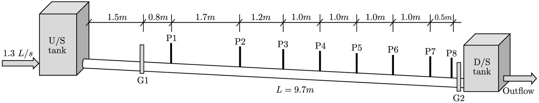
The experimental setup for Trajkovic et al. (1999) consists of a 10 m pipe with an inner diameter of 0.1 m that is connected to upstream and downstream tanks with two intervening sluice gates. Head at the upstream tank was kept constant during the experiments and an upstream sluice gate (G1) located 1.5 m from the tank was used to control the flow. Herein, we focus on their Type A experiments where the downstream tank was in a supercritical overflow condition. The downstream gate (G2), located 0.4 m upstream of the downstream tank, was modulated during the experiments to create transient flows. To restrict possible air-water interaction in the pressurized flow, several vents were located at the top of the pipe. Pressure transducers were placed along the length of the pipe to measure head at eight location. Fig. 6 shows their experimental setup and the pressure measurement locations. The Manning roughness coefficient for the pipe reported by Trajkovic et al. (1999) was . The upstream boundary conditions and gate G2 openings for Case A experiments are summarized in Table 1.
| Type | Slope | Upstream Q () | G1 height (m) | G2 initial height (m) | G2 reopen height (m) | G2 time closed (s) |
|---|---|---|---|---|---|---|
| A1 | 0.027 | 0.0013 | 0.014 | 0.100 | 0.008 | 30.0 |
| A2 | 0.027 | 0.0013 | 0.014 | 0.100 | 0.015 | 30.0 |
| A3 | 0.027 | 0.0013 | 0.014 | 0.100 | 0.028 | 30.0 |
| A4 | 0.014 | 0.0013 | 0.014 | 0.100 | 0.100 | 30.0 |
Source: Data from Trajkovic et al. (1999).
Our numerical domain to mimic this experiment was subdivided into 55 elements of 0.185 m length. The DPS model uses the Manning’s of Trajkovic et al. (1999) without calibration. The supercritical downstream boundary conditions are approximated herein by extending the pipe section downstream of gate G2 by 1 m and adding a 5 m buffer domain. The extended pipe and buffer section is subdivided into 30 elements of 0.2 m length. The buffer domain has zero slope and a larger Manning’s roughness coefficient () to damp numerically reflected waves at the downstream boundary.
For the DPS model, sluice gates G1 and G2 are modeled as gated side orifices as in EPA SWMM with the standard orifice flow equations from Brater and King (1996)where is the orifice discharge coefficient; is the area of the orifice opening; and is the effective head across the orifice. The discharge coefficient was used without any calibration. When any of the orifice is unsubmerged the flow is modeled as a weir flow according to EPA SWMM and thus, the equivalent weir equations were used to model the flow () aswhere is the crest length; and is the weir coefficient, which is estimated aswhere is the pipe diameter.
(26)
(27)
(28)
The numerical model in Trajkovic et al. (1999) that accompanied their experiments used a Preissmann Slot approach with a fixed slot width of , which corresponds to using Eq. (1). They reported using due to numerical instabilities that appeared with a narrower slot. Our model used , which is similar to the expected acoustic celerity. The Preissmann Number decay time scale was set to , which is 20% of the gate closing time. The entire pressurization event of the experiment is . The surcharge shock parameter was set as , which results in a incipient surcharge celerity, and .
Type A1-3 Experiment Comparisons
Trajkovic et al. (1999) reported laboratory-observed pressure head measurements at sensor location P5 and P7 for experiments A1 through A3. Fig. 7 shows the pressure head comparison between our model and experiments at sensor location P5, which is 2.6 m upstream of gate G2. Fig. 8 shows similar data for location P7. At both locations the simulated pressure heads are in good agreement with the experimental result during the filling bore (). Note that DPS simulations of three test cases have identical pressure heads during bore filling since the differences between these three test cases (see Table 1) are only in the G2 gate opening heights after 30 s. For , the DPS model has reasonable agreement for the initial pressure drop with gate opening and the subsequent recovery phase for all the test cases at the P5 and P7 sensors. We note that the pressure behavior in the modeled A3 case is slightly different than the A1 and A2 cases for the recovery phase; whereas A1 and A2 show slight overprediction of the recovery pressure, the A3 case shows slight underprediction. We suspect this disagreement is related to the larger pressure drop and recovery spike occurring in the first few seconds after the gate is opened in Case A3. Also note that at location P7 (closer to the gate G2), as shown in Fig. 8, the upstream propagating bore in the DPS model and laboratory observations are almost identical. However, as the bore moves upstream to location P5 (see Fig. 7) the bore in the model arrives a few seconds sooner than observed in the experiment. This divergence is attributable to the fact that the numerical model includes dispersive errors, which bias the wave speed and accumulate position error as waves propagate through space.

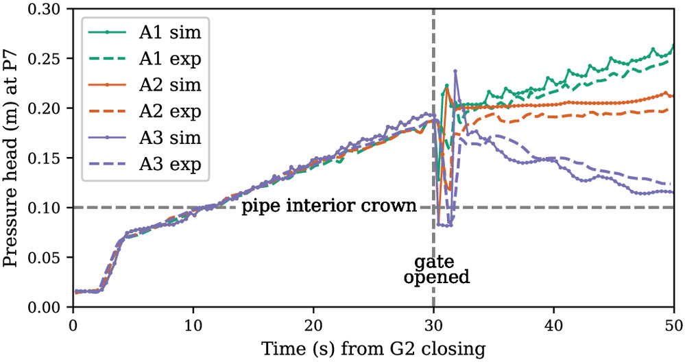
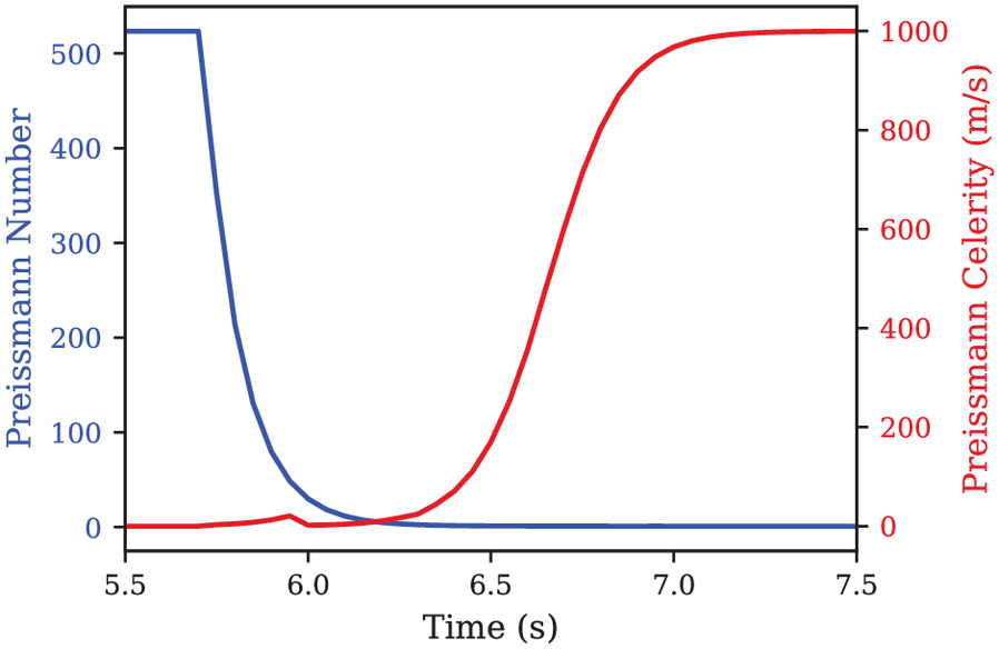
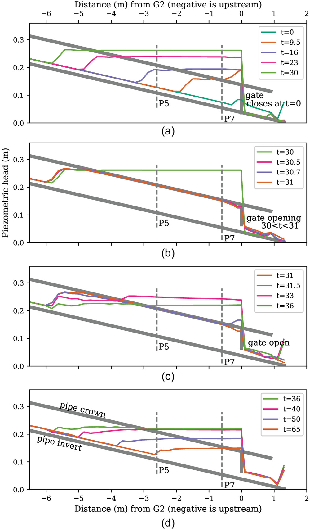
Fig. 9 shows the evolution of and at sensor location P7 for the experiment A3, illustrating the model’s ability to produce smooth increases in during pressurization ( and ) while allowing sharp decrease in during depressurization (). To provide further insight, Fig. 10 illustrates the evolution of the piezometric head profiles for DPS simulations of the A3 experiment. In Fig. 10(a), the upstream-propagating bore forms with the gate closure and arrives at P7 later. During the rapid gate opening, Fig. 10(b), we see a rapid reduction of head that is followed in Fig. 10(c) by a rebound of the pressure head as the filling bore reverses and water begins to accelerate back down the pipe.

Type A4 Experiment Comparisons
The Trajkovic et al. (1999) experiment A4 used a shallower bed slope than cases A1-A3 and fully-opened gate G2 after 30 s (see Table 1). The Trajkovic et al. (1999) paper reported the evolution of the filling bore from sensors P3 through P7, as shown in Fig. 11. The new DPS model correctly estimates bore propagation time for P6 and P7, close to the gate. However, as in Fig. 7 for case A1-A3, the simulated bore arrives earlier than observed at locations P3–P5, with the discrepancy indicating the model bore biased toward a faster bore wave celerity that accumulates error in the front arrival time. Similar phase error was observed in the Hodges (2020) model of the same experiments. Additionally, the model slightly overpredicts the pressure heads for all the sensors when the bore first arrives, perhaps indicating that the model dissipation rate is not optimized. No attempt has been made to calibrate Manning’s for the DPS in this model.

Discussion
The DPS method provides a means of smoothing the numerical pressure celerity across a celerity shock to prevent oscillations that typically occur whenever there are mixed-flow transitions conditions or pipe size changes. A key point is that celerity shocks are not necessarily numerical artifacts, but are part of the physics of transitions in acoustic celerity. However, the large oscillations often seen in models of mixed-flow shocks are predominantly numerical artifacts occurring in response to the physical shock.
With the notable exception of Kerger et al. (2011), the primary methods for handling the celerity shock and resulting numerical oscillations in transient-storage models have been either (1) limit the modeled acoustic celerity to reduce the shock and hence limit oscillations, or (2) provide some form of damping to prevent oscillations from growing. For example, Trajkovic et al. (1999) presented a Preissmann Slot model of their laboratory experiments that used a low acoustic celerity () to minimize the postshock oscillations generated by the rapid opening/closing of the gate. The TPA approach of Vasconcelos et al. (2006) was able to operate at an order of magnitude higher celerity () but encountered oscillations when attempting to model at acoustic celerities. Extending the TPA approach, Vasconcelos et al. (2009) proposed new filtering strategies and added dissipation to damp oscillations for even higher celerities. Similarly, Malekpour and Karney (2015) proposed an enhanced numerical viscosity that damped oscillations. For large-scale networks, the TPA method applied with an approximate Riemann solver in Sanders and Bradford (2010) encountered postshock oscillations when acoustic celerities were used, although high frequency oscillations were reduced by using a coarse model grid (effectively increasing numerical dissipation). Oscillations have also been addressed through development of numerical solvers with enhanced dissipative behavior, as in An et al. (2018), where the dissipative MINMOD limiter was used in a hybrid solver combining an upwind discretization at shocks and a more dissipative centered discretization elsewhere, which successfully limited oscillations for celerities less than . Similarly, León et al. (2009) applied the dissipative MINMOD limiter with an approximate Riemann solver and achieved success at acoustic-scale celerities; however, their success is arguably due to their tapered Preissmann Slot, which serves to locally-reduce celerities at the mixed-flow transition hence limiting the shock and the source of oscillations.
The interesting exception to the preceding discussion is the model of Kerger et al. (2011), which appears to be the only transient storage model that uses acoustic celerities without some form of damping and/or smoothing. To the best of our knowledge, the key change from other Godunov solvers is that Kerger et al. (2011) uses an exact rather than an approximate Riemann solver. However, it is not clear how the exact Riemann solver might eliminate shock oscillations that occur with the approximate solver. This issue requires further investigation for traditional Godunov methods.
The new DPS algorithm is similar to prior works where the surcharge celerity is reduced to smooth celerity shocks—but instead of a global limit on the surcharged celerity we provide local smoothing in time and space across any celerity transition, which allows the transition to develop without oscillations and does not require artificial damping. In the DPS algorithm the celerity smoothing is accomplished by smoothing the evolution of the Preissmann number in time and space, which affects the relationship between surcharge head and the transient storage volume of the Preissmann Slot. It seems likely that other forms of transient storage solvers might be able to similarly reduce oscillations with ad hoc smoothing for acoustic celerity.
Of course, the DPS algorithm does not solve the time-scale challenge of mixed-flow modeling. High acoustic celerities require extremely small time steps in an explicit numerical scheme to to meet the CFL limit [Eq. (7)]. For the SWMM5+ model (used herein) with the DPS algorithm for a target celerity of , the Vasconcelos et al. (2006) test case required for CFL with element sizes of 3.6 cm. To maintain the CFL for the Trajkovic et al. (1999) test case, the 20 cm elements required . For practical stormwater system simulations, such small time steps are impractical, so modelers will typically need to select their as a compromise between fidelity to small time-scale physics and computational constraints. Indeed, this idea has been previously recognized, as Sanders and Bradford (2010) suggested pressurized flow wave speeds in the range of might be most suitable for storm sewer flow modeling. If we consider the lower end of this range as a and take 50 m as a typical conduit discretization scale, then a model time step of 1.0 s will likely be suitable. Although this is perhaps smaller than we might wish, it will likely be a practical for simulations conducted on multi-core computers.
The DPS algorithm introduces three parameters () in place of the single “slot width” parameter for the conventional Preissmann Slot. As discussed in the section on Nondimensionalizing the Priessmann Slot and illustrated in Eq. (7), the can be set based on the CFL limit of the numerical algorithm, expected flow velocity, discretization length, and the target time step. However, in this introductory work, we have not attempted to fully examine the implications of and upon the solution. Our preliminary observations are the surcharge shock parameter () does not exert a major control, and can be set as for a wide variety of conditions. In contrast, the decay time scale, , has a direct effect on the stability of the simulation and its value will affect the damping rate of postshock oscillations. Formally, the controls how fast the is converging to through Eq. (22). Alternatively, it can be thought of as the time scale for . In general, a small value of implies a rapidly changing transition and may allow a celerity shock to generate numerical oscillations. A preliminary investigation into the effect of on the solution of the Vasconcelos et al. (2006) test case is illustrated in Fig. 12. For this case, values of are fairly similar, but results in dramatic spatial oscillations in Piezometric head. It can be seen that higher values of (e.g., ) tend to slightly slow the bore propagation speed, resulting in a shorter distance traveled in the snapshot. As decreases, we see a relatively smooth bore being retained until , where incipient oscillations appear near the bore front. For context, was used in the TPA simulations of Vasconcelos et al. (2006) presented in Fig. 4. In contrast, our simulations of the Trajkovic et al. (1999) test case used . In both cases the damping time scales are far larger than the model time steps required for stability. As a cautionary note, both the test cases presented herein are of similar length scale and used similar . Thus, we cannot presently draw conclusions as to the appropriate setting of in more general cases, especially for network-scale simulations or with lower . It seems likely that an automated approach for selecting could be related to the target model time step, , the discrete element length, and the physical time scales of the system.

If the DPS approach has a disadvantage, it is the same as the underlying Preissmann Slot idea: the acoustic celerity must be known (or approximated) prior to setting the slot parameters; i.e., as the DPS is presently posed, the acoustic celerity cannot be part of the solution of the algorithm. Thus, where transient modeling is focused on relationships between pipe elasticity and acoustic wave speed, the DPS model as presently formulated cannot replace classic hydraulic transient solvers.
The main advantages of the DPS approach are (1) ensuring a smooth solution across a celerity shock, and (2) providing consistent celerities throughout the system. These characteristics should provide more flexible and robust system-level solutions under mixed-flow conditions. Nevertheless, modeling mixed-flow conditions for large networks will remain a challenge due to the wide range of scales and the need to use small time steps to resolve acoustic celerities. Furthermore, the physics of subatmospheric pressure (Vasconcelos et al. 2006; Kerger et al. 2011) and air entrapment (Vasconcelos and Marwell 2011; Kerger et al. 2012) have yet to be considered within the DPS framework. Our near-term goals for DPS include investigating the application of DPS at network scale and developing automated approaches to setting parameters and .
Conclusion
A new DPS algorithm is presented to solve some of the long-standing problems associated with oscillations of the modeled pressure heads at mixed-flow transitions. The new approach replaces the traditional specification of a Preissmann Slot width with three parameters, the surcharge shock parameter (), a decay time scale () and a target celerity (). The key advance of the DPS method is defining the Preissmann Slot behavior across a transition using a smoothed Preissmann Number, which is a new nondimensional number introduced for this purpose. Formally, the Preissmann Number is an inverse Mach Number that relates the target celerity to the local Preissmann Slot celerity. Although several questions remain as to the selection of parameters , , and for large network simulations, the new DPS algorithm shows promise for reducing numerical oscillation in mixed-flow simulations of storm sewer systems while retaining the relative simplicity of the Preissmann Slot method.
Data Availability Statement
The version of the SWMM5+ code and all supporting data used in the previous simulations are archived in the Texas Data Repository at https://doi.org/10.18738/T8/I5KDRX (Sharior et al. 2022). The SWMM5+ code is under active development as public domain software with the latest version developed by the Center for Infrastructure Modeling and Management available at https://github.com/CIMM-ORG/SWMM5plus. Additional methodology and discussion supporting this work will be found in the associated technical report, Sharior et al. (2023).
Acknowledgments
This article is based upon work supported by the National Science Foundation under Grants Nos. 2049025 and 2048607 and was developed in part under Cooperative Agreement No. 83595001 awarded by the US Environmental Protection Agency to The University of Texas at Austin. It has not been formally reviewed by EPA. The views expressed in this document are solely those of the authors and do not necessarily reflect those of the Agency. EPA does not endorse any products or commercial services mentioned in this publication.
References
An, H., S. Lee, S. J. Noh, Y. Kim, and J. Noh. 2018. “Hybrid numerical scheme of Preissmann slot model for transient mixed flows.” Water 10 (7): 899. https://doi.org/10.3390/w10070899.
Brater, E. F., and H. W. King. 1996. Handbook of hydraulics. 7th ed. New York: McGraw-Hill.
Capart, H., X. Sillen, and Y. Zech. 1997. “Numerical and experimental water transients in sewer pipes.” J. Hydraul. Res. 35 (5): 659–672. https://doi.org/10.1080/00221689709498400.
Cardle, J. A., and C. C. S. Song. 1988. “Mathematical-modeling of unsteady-flow in storm sewers.” Int. J. Eng. Fluid Mech. 1 (4): 495–518.
Cunge, J. A., and M. Wegner. 1964. “Intégration numérique des équations d’écoulement de Barré de Saint-Venant par un schéma implicite de différences finies.” Houille Blanche 50 (1): 33–39. https://doi.org/10.1051/lhb/1964002.
Garcia-Navarro, P., F. Alcrudo, and A. Priestley. 1994. “An implicit method for water flow modelling in channels and pipes.” J. Hydraul. Res. 32 (5): 721–742. https://doi.org/10.1080/00221689409498711.
Guo, Q., and C. C. Song. 1990. “Surging in urban storm drainage systems.” J. Hydraul. Eng. 116 (12): 1523–1537. https://doi.org/10.1061/(ASCE)0733-9429(1990)116:12(1523).
Hodges, B. R. 2020. “An artificial compressibility method for 1D simulation of open-channel and pressurized-pipe flow.” Water 12 (6): 1727. https://doi.org/10.3390/w12061727.
Hodges, B. R., and F. Liu. 2020. “Timescale interpolation and no-neighbor discretization for a 1D finite-volume Saint-Venant solver.” J. Hydraul. Res. 58 (5): 738–754. https://doi.org/10.1080/00221686.2019.1671510.
Hodges, B. R., S. Sharior, E. Tiernan, G. R. Briceno, E. Jenkins, C. Brashear, and C. E. D. Hernandez. 2023. The SWMM5+ hydraulic engine. Austin, TX: Univ. of Texas at Austin.
Hodges, B. R., J. G. Vasconcelos, S. Sharior, and V. Geller. 2022. “Hyperbolic numerical models for unsteady incompressible, surcharged stormwater flows.” In Proc. 39th IAHR World Congress, 4061–4066. Beijing: International Association for Hydro-Environment Engineering and Research.
Ji, Z. 1998. “General hydrodynamic model for sewer/channel network systems.” J. Hydraul. Eng. 124 (3): 307–315. https://doi.org/10.1061/(ASCE)0733-9429(1998)124:3(307).
Kerger, F., P. Archambeau, B. J. Dewals, S. Erpicum, and M. Pirotton. 2012. “Three-phase bi-layer model for simulating mixed flows.” J. Hydraul. Res. 50 (3): 312–319. https://doi.org/10.1080/00221686.2012.684454.
Kerger, F., P. Archambeau, S. Erpicum, B. J. Dewals, and M. Pirotton. 2011. “An exact Riemann solver and a Godunov scheme for simulating highly transient mixed flows.” J. Comput. Appl. Math. 235 (8): 2030–2040. https://doi.org/10.1016/j.cam.2010.09.026.
Leon, A. S., M. S. Ghidaoui, A. R. Schmidt, and M. H. García. 2008. “Efficient second-order accurate shock-capturing scheme for modeling one- and two-phase water hammer flows.” J. Hydraul. Eng. 134 (7): 970–983. https://doi.org/10.1061/(ASCE)0733-9429(2008)134:7(970).
León, A. S., M. S. Ghidaoui, A. R. Schmidt, and M. H. Garcia. 2010. “A robust two-equation model for transient-mixed flows.” J. Hydraul. Res. 48 (1): 44–56. https://doi.org/10.1080/00221680903565911.
León, A. S., M. S. Ghidaoui, A. R. Schmidt, and M. H. García. 2009. “Application of Godunov-type schemes to transient mixed flows.” J. Hydraul. Res. 47 (2): 147–156. https://doi.org/10.3826/jhr.2009.3157.
Lieb, A. M., C. H. Rycroft, and J. Wilkening. 2016. “Optimizing intermittent water supply in urban pipe distribution networks.” SIAM J. Appl. Math. 76 (4): 1492–1514. https://doi.org/10.1137/15M1038979.
Malekpour, A., and B. W. Karney. 2015.“Spurious numerical oscillations in the Preissmann slot method: Origin and suppression.” J. Hydraul. Eng. 142 (3): 04015060. https://doi.org/10.1061/(ASCE)HY.1943-7900.0001106.
Preissmann, A., and J. A. Cunge. 1961. “Calcul du mascaret sur machine électronique.” Houille Blanche 47 (5): 588–596. https://doi.org/10.1051/lhb/1961045.
Rokhzadi, A., and M. Fuamba. 2022. “A modified shock tracking–capturing finite-volume approach for transient mixed flows in stormwater systems.” J. Hydraul. Eng. 148 (11): 04022022. https://doi.org/10.1061/(ASCE)HY.1943-7900.0001997.
Rossman, L. A. 2017. Storm water management model reference manual, Volume II—Hydraulics. Cincinnati: USEPA, National Risk Management Laboratory, Office of Research and Development.
Sanders, B. F., and S. F. Bradford. 2010. “Network implementation of the two-component pressure approach for transient flow in storm sewers.” J. Hydraul. Eng. 137 (2): 158–172. https://doi.org/10.1061/(ASCE)HY.1943-7900.0000293.
Sharior, S., B. R. Hodges, and J. G. Vasconcelos. 2022. Replication data for the generalized, dynamic transient-storage form of the Preissmann slot. Austin, TX: Texas Data Repository. https://doi.org/10.18738/T8/I5KDRX.
Sharior, S., B. R. Hodges, and J. G. Vasconcelos. 2023. Background and details of the generalized, dynamic, transient-storage form of the Preissmann slot. Austin, TX: Texas Data Repository.
Sjöberg, A. 1982. “Sewer network models DAGVL-A and DAGVL-DIFF.” In Urban stormwater hydraulics and hydrology, edited by B. C. Yen, 127–136. Littleton, CO: Water Resource Publications.
Song, C. C. S., J. A. Cardle, and K. S. Leung. 1983. “Transient mixed flow models for storm sewers.” J. Hydraul. Eng. 109 (11): 1487–1504. https://doi.org/10.1061/(ASCE)0733-9429(1983)109:11(1487).
Trajkovic, B., M. Ivetic, F. Calomino, and A. D’Ippolito. 1999. “Investigation of transition from free surface to pressurized flow in a circular pipe.” Water Sci. Technol. 39 (9): 105–112. https://doi.org/10.2166/wst.1999.0453.
USEPA. 2022. “SWMM 5 updates and bug fixes (txt).” Accessed December 15, 2022. https://www.epa.gov/system/files/other-files/2022-08/epaswmm5_updates_0.txt.
Vasconcelos, J., Y. Eldayih, Y. Zhao, and J. A. Jamily. 2018. “Evaluating storm water management model accuracy in conditions of mixed flows.” J. Water Manage. Model. 26: C451.
Vasconcelos, J., and S. J. Wright. 2004. “Numerical modeling of the transition between free surface and pressurized flow in storm sewers.” In Proc., Innovative Modeling of Urban Water Systems, edited by W. James, 189–214. Guelph, ON, Canada: Computational Hydraulics International Publications.
Vasconcelos, J. G., and D. T. Marwell. 2011. “Innovative simulation of unsteady low-pressure flows in water mains.” J. Hydraul. Eng. 137 (11): 1490–1499. https://doi.org/10.1061/(ASCE)HY.1943-7900.0000440.
Vasconcelos, J. G., and S. J. Wright. 2007. “Comparison between the two-component pressure approach and current transient flow solvers.” J. Hydraul. Res. 45 (2): 178–187. https://doi.org/10.1080/00221686.2007.9521758.
Vasconcelos, J. G., S. J. Wright, and P. L. Roe. 2006. “Improved simulation of flow regime transition in sewers: Two-component pressure approach.” J. Hydraul. Eng. 132 (6): 553–562. https://doi.org/10.1061/(ASCE)0733-9429(2006)132:6(553).
Vasconcelos, J. G., S. J. Wright, and P. L. Roe. 2009. “Numerical oscillations in pipe-filling bore predictions by shock-capturing models.” J. Hydraul. Eng. 135 (4): 296–305. https://doi.org/10.1061/(ASCE)0733-9429(2009)135:4(296).
Wylie, E. B., and V. L. Streeter. 1983. Fluid transients. Ann Arbor, MI: FEB Press.
Zhou, F., F. E. Hicks, and P. M. Steffler. 2002. “Transient flow in a rapidly filling horizontal pipe containing trapped air.” J. Hydraul. Eng. 128 (6): 625–634. https://doi.org/10.1061/(ASCE)0733-9429(2002)128:6(625).
Information & Authors
Information
Published In

Journal of Hydraulic Engineering
Volume 149 • Issue 11 • November 2023
Copyright
This work is made available under the terms of the Creative Commons Attribution 4.0 International license, https://creativecommons.org/licenses/by/4.0/.
History
Received: Dec 15, 2022
Accepted: May 9, 2023
Published online: Sep 6, 2023
Published in print: Nov 1, 2023
Discussion open until: Feb 6, 2024
ASCE Technical Topics:
- Continuum mechanics
- Cross sections
- Dynamic models
- Dynamics (solid mechanics)
- Engineering fundamentals
- Engineering mechanics
- Flow (fluid dynamics)
- Fluid dynamics
- Fluid mechanics
- Hydrologic engineering
- Infrastructure
- Mathematics
- Models (by type)
- One-dimensional flow
- Pipe flow
- Pipeline systems
- Pipes
- Pressure pipes
- Solid mechanics
- Transient flow
- Transient response
- Water and water resources
Authors
Metrics & Citations
Metrics
Citations
Download citation
If you have the appropriate software installed, you can download article citation data to the citation manager of your choice. Simply select your manager software from the list below and click Download.