Surfing Waves from the Ocean to the River with the Serre-Green-Naghdi Equations

Cienfuegos, Rodrigo

doi:10.1061/JHEND8.HYENG-13487

Open access

Technical Papers

Jul 3, 2023

Surfing Waves from the Ocean to the River with the Serre-Green-Naghdi Equations

Author: Rodrigo Cienfuegos, Ph.D. https://orcid.org/0000-0001-5768-2477 [email protected]Author Affiliations

Publication: Journal of Hydraulic Engineering

Volume 149, Issue 9

https://doi.org/10.1061/JHEND8.HYENG-13487

PDF

Abstract

A wide variety of hydraulic and coastal flows can be modeled using shallow water theories, where the so-called Serre-Green-Naghdi (SGN) equations constitute a fully nonlinear and weakly dispersive wave theory that has been successfully applied in fluvial and maritime contexts. In the present contribution, we show that SGN models with wave-breaking parameterizations can reproduce challenging nonlinear processes in the surf and swash zones including wave–wave interactions and infragravity wave generation from a narrow-band swell spectrum. The excellent performance of the model motivates us to explore its application to a simplified shallow bar-built river configuration where surf zone–generated infragravity waves may propagate upstream the river. We show that long-wave penetration is controlled by the Froude number over the bar, and that these nonlinear long waves may give rise to a solitonic dynamics. The power spectral density (PSD) signature of free surface time series with a slope of

\sim f^{- 1}

in the infragravity range is consistent with the latter, as also found in field observations. Transferring of energy into lower frequencies is observed in the numerical experiment as long waves propagate upstream; nevertheless, low-frequency energy also cascades back into the swell energy band. Standard linear Fourier analysis may fail in showing the hidden solitonic dynamics, so nonlinear techniques would need to be applied to fully elucidate the fate of the long-wave energy while propagating upstream of river mouths.

Introduction

A wide variety of hydraulic and coastal flows can be modeled using shallow-water theories. Shallow-water wave approximations can be derived from the inviscid and incompressible Euler or potential flow equations (when the flow is in addition assumed irrotational), using, for instance, series of expansion based on the following standard nondimensional parameters:

ϵ = \frac{H}{h} and δ = \frac{h}{λ}

(1)

then truncating and depth integrating the resulting equations to obtain the so-called Boussinesq-type (BT) water wave models [see reviews from Brocchini (2013) and Kirby (2016)]. In Eq. (1),

H

,

h

, and

λ

respectively represent a typical wave height, the mean depth of the fluid, and a characteristic wavelength in the horizontal dimension. Parameters

ϵ

and

δ

measure the strength of nonlinearity and frequency dispersion, respectively. Similary, the Ursell number,

U_{r}

, and the wave steepness,

Λ

, are derived from them, such that

U_{r} = \frac{ϵ}{δ^{2}} = \frac{H λ^{2}}{h^{3}}, Λ = ϵ δ = \frac{H}{λ}

(2)

Shallow-water wave models can also be obtained by depth averaging the Reynolds equations so turbulent and mixing terms may be naturally incorporated; the equations are nondimensionalized based on the same scaling in Eq. (1), and higher-order terms are truncated under shallow-water assumptions [see, for instance, Kim and Lynett (2011) and Kim (2015)]. BT models incorporating both turbulent and rotational dynamics have also been derived and implemented for surf zone applications (Briganti et al. 2004; Musumeci et al. 2005).

The Ursell number measures the relative importance of nonlinear effects in comparison to dispersion and can be used to distinguish between different water wave theories. For waves of finite amplitude,

U_{r} ≫ 1

corresponds to the nondispersive nonlinear approximation of Barré de Saint-Vénant (1871),

U_{r} \sim O (1)

denotes the weakly dispersive nonlinear theory of Boussinesq (1872) and Korteweg and de Vries (1895), and

U_{r} ≪ 1

corresponds to the linear dispersive approximation of Airy (1841). When

ϵ \sim O (1)

, large-amplitude waves propagating in shallow waters can be modeled. The first strongly nonlinear, weakly dispersive set of BT equations was derived by Serre (1953), Su and Gardner (1969), and Green and Naghdi (1976) obtained the same set of equations following a different approach. The Serre-Green-Naghdi (SGN) equations can be obtained by depth averaging the incompressible, irrotational, and inviscid flow equations and truncating the resulting set of equations at

O (δ^{4})

without making any assumptions on the order of

ϵ

(Barthélemy 2004). This full nonlinearity makes the SGN equations ideal for studying large-amplitude or nearly breaking waves propagating in shallow waters, but boundary-layer effects and breaking dissipation need to be introduced through ad hoc formulations.

The work of Serre (1953) was aimed to extend the range of application of the nondispersive Saint-Venant equations in open-channel hydraulics by allowing vertical accelerations in the fluid motion (i.e., dropping the hydrostatic pressure distribution assumption); free-surface waves propagating in open-channel flows such as the ones that could appear in weak hydraulic jumps, the sudden operation of weirs and gates, and the flow over spillways or below sluice gates were among Serre’s main concerns. Curiously, it was not until the last couple of decades that this set of equations started to be applied again to the problems first sought by Serre (e.g., Nadiga et al. 1996; Mohapatra and Chaudhry 2004; Mignot and Cienfuegos 2009; Kim and Lynett 2011; Cantero-Chinchilla et al. 2016; Shimozono et al. 2017; Roy Biswas et al. 2021). Indeed, BT equations had to come a long way in coastal and maritime theory and practice since the work of Peregrine (1967), who set the basis for engineering and computational physics to undertake a thorough and exciting exploration of the potentialities of nonlinear shallow-water wave theories, before coming back to the open-channel hydraulics arena where they were first born.

In their way back home, BT equations have demonstrated their elegance, versatility, and accuracy over a wide range of coastal applications; to do so, specific numerical methods, boundary conditions, means of incorporating wave-breaking dynamics, and higher computing power were made available. Complete reviews on these advancements are presented by Brocchini (2013) and Kirby (2016).

In the present contribution, we explore the application of the set of SGN equations to surf zone processes involving infragravity wave generation and their penetration into river mouths. Recent field observations in shallow bar-built estuaries have shown that while sea-swell energy is mostly dissipated in the surf zone, low-frequency energy in the range of the infragravity band could propagate upstream of river mouths (e.g., Williams and Stacey 2016; Bertin et al. 2019; McSweeney et al. 2020; Brocchini 2020). In the following, we present the SGN numerical model and test its capabilities under a challenging surf zone laboratory experiment with infragravity wave generation. The excellent performance of the model motivates us to explore its application to river mouth processes including surf zone–generated infragravity waves penetrating upstreams.

Material and Methods

Serre-Green-Naghdi Numerical Model for Breaking and Nonbreaking Waves

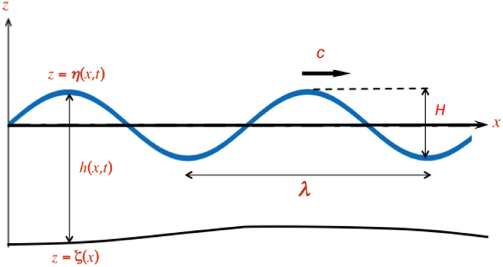
The numerical results presented herein were obtained using the fourth-order finite-volume solver SERR-1D (Cienfuegos et al. 2006, 2007), which numerically integrates the set of Serre-Green-Naghdi fully nonlinear and weakly dispersive shallow-water equations (Serre 1953; Green and Naghdi 1976). The equations are recast in the following form:

h_{t} + F_{x} = D_{h}

(3)

q_{t} + G_{x} = \frac{1}{h} D_{h u} - \frac{τ_{b}}{ρ h} - S

(4)

where

ρ

= water density;

h

= water depth;

τ_{b}

= bed shear stress; and subscripts

t

and

x

= partial derivatives with respect to time and space, respectively. In addition,

D_{h}

and

D_{h u}

represent breaking dissipation terms to be described subsequently. Both terms are written in a strict conservative form so when spatially integrated over the breaker front, neither mass nor momentum are added or subtracted (Cienfuegos et al. 2010a). The current breaking dissipation model was designed to overcome a limitation observed when implementing the Kennedy et al. (2000) model (which only considers a diffusive term in the momentum equation) in the SGN set of equations: it was not possible to accurately obtain the wave height and wave asymmetry evolution in the surf zone at the same time by tuning the model parameters. The latter is shown and discussed in Cienfuegos et al. (2010a, Fig. 3), and motivated the inclusion of an additional term in the mass conservation equation. The remaining variables and functions are defined as follows:

q = [1 + (h_{x} + ζ_{x}) ζ_{x} + \frac{1}{2} h ζ_{x x})] u - \frac{1}{3 h} {(h^{3} u_{x})}_{x} - α ζ^{2} u_{x x}

(5)

F = h u

(6)

G = q u + g (h + ζ) - \frac{1}{2} u^{2} (1 + ζ_{x}^{2}) + (ζ_{x} u - \frac{1}{2} h u_{x}) h u_{x} - α ζ^{2} u_{x}^{2} + u u_{x x} + g {(h + ζ)}_{x x}

(7)

S = 2 α ζ ζ_{x} u u_{x} + g {(h + ζ)}_{x x}

(8)

where

g

= acceleration of gravity;

u

= depth-averaged horizontal velocity;

z = ζ

is the vertical coordinate of the impermeable bed, measured from the still water depth (

z

is positive upward, see Fig. 1); and

α

= dispersion correction parameter set to

α = 1 / 15

to produce a Padé approximant to the linear Stokes dispersion relation (Cienfuegos et al. 2007).

Fig. 1. Variables describing the wave propagation over uneven bathymetries.

Breaking energy dissipation is taken into account through the diffusive-type terms,

D_{h}

and

D_{h u}

, applied locally on the wave front face using the hydraulic jump analogy on a frame of reference attached to each wave crest as described in Cienfuegos et al. (2010a). An explicit breaking criterion based on the breaker angle such as the one proposed by Schäffer et al. (1993) is considered to switch these terms on and off. The mathematical form for

D_{h}

and

D_{h u}

is chosen to ensure the overall mass and momentum budget is preserved, acting only as to locally redistribute these quantities under the breaker (Cienfuegos et al. 2010a). Breaking terms are thus written in the form

D_{h} = \frac{\partial}{\partial x} (ν_{h} h_{x})

(9)

D_{h u} = \frac{\partial}{\partial x} [ν_{h u} {(h u)}_{x}]

(10)

where

ν_{h}

and

ν_{h u}

are diffusivity functions varying locally on each breaking wave (Cienfuegos et al. 2010a)

ν_{h} (X) = - K_{h} \exp (\frac{X}{l_{r}} - 1) (\frac{X}{l_{r}} - 1) + {(\frac{X}{l_{r}} - 1)}^{2}

(11)

ν_{h u} (X) = - K_{h u} \exp (\frac{X}{l_{r}} - 1) (\frac{X}{l_{r}} - 1) + {(\frac{X}{l_{r}} - 1)}^{2}

(12)

with

K_{h}

and

K_{h u}

slowing varying scaling coefficients;

X

= moving horizontal coordinate attached to the wave crest of the breaker; and

l_{r}

= horizontal extent over which breaking terms are active. The adoption of an exponential distribution for the eddy viscosity functions on the breaker fronts attempts to facilitate the physical interpretation of the parameterization of the ad hoc diffusive-like terms using the hydraulic jump analogy. The default values for model parameters proposed by Cienfuegos et al. (2010a) are

K_{h} = 2 c_{0} d

,

K_{h u} = 20 c_{0} d

, and

l_{r} / d = 0.82

, where

c_{0} = \sqrt{g d}

is the linear shallow-water phase speed computed with the local still-water depth,

d = | ζ |

. Similarly, breaking inception occurs when the mean front breaker angle,

θ

, reaches

θ_{b} = 30 °

and stops when it falls below 8°.

The bed shear stress in Eq. (4) is estimated through a quadratic friction model (Grant and Madsen 1979)

τ_{b} = \frac{1}{2} C_{f} ρ u | u |

(13)

where

C_{f}

= empirical Darcy-Weisbach friction factor, which may be expressed in terms of the open-channel Manning friction coefficient,

n

, as [see, for instance, Julien (2010)]

C_{f} = \frac{2 g n^{2}}{h^{1 / 3}}

(14)

For nearshore wind waves, values for

C_{f}

are in the order of

10^{- 3}

[see, for instance, Church and Thornton (1993)], while in hydraulics the Manning coefficient

n

ranges between 0.012 and 0.035 for straight channels with sandy beds [see, for instance, Arcement and Schneider (1989)].

The numerical implementation of the model includes absorbing-generating boundary conditions to specify an incoming wave field and let the reflected or outgoing waves to leave the domain freely, a moving shoreline boundary condition to represent wet–dry interfaces, and the possibility of specifying flow discharge or gate operation functions to address hydraulic problems (Cienfuegos et al. 2007; Mignot and Cienfuegos 2009). A fourth-order numerical finite-volume scheme is used to discretize the quasi-conservative form of the SGN [Eqs. (3) and (4)], where cell-face values are reconstructed using implicit compact schemes, the nonconservative source terms are discretized using a fourth-order centered-in-space approach, and time integration is performed using a fourth-order Runge-Kutta method; details and an extensive analysis of the numerical scheme are presented in Cienfuegos et al. (2006). The model has shown its accuracy and validity on coastal and hydraulic applications (Cienfuegos et al. 2007, 2010a; Mignot and Cienfuegos 2009; Michallet et al. 2011; Bonneton et al. 2011; Moris et al. 2021).

Experimental Setup for Infragravity Waves Generation in the Surf Zone

The laboratory experiments presented here were carried out in the wave tank of the Instituto Nacional de Hidráulica in Peñaflor, Chile (INH) (Cienfuegos et al. 2010b). The wave flume is 70 m long and has a square cross section with side length of 1.5 m. It has a concrete bottom and side walls and was prepared with an impermeable smooth concrete plane beach of 1/80 slope. The beach starts 23 m from the mean position of the wave paddle and the origin for the horizontal coordinate,

x

, is taken at the commencement of the slope, positive shoreward. The origin for the vertical coordinate,

z

, is taken at the still-water level, positive upward (Fig. 2). The flume is equipped with a hydraulically driven piston-type wave paddle from the Danish Hydraulic Institute (DHI). The generator is controlled by the DHI wave synthesizer software and allows for second-order wave generation (Schäffer 1996), which significantly suppresses spurious free waves. In addition, back reflection at the wave paddle is minimized by active absorption through the DHI Active Wave Absorption Control System (AWACS). The wave signal is highly repeatable, allowing for data collection at multiple locations in the wave flume.

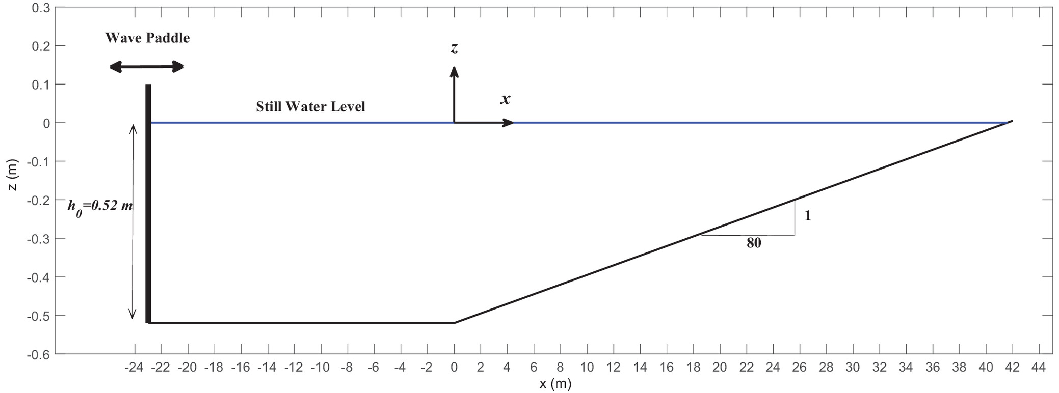
A large number of experiments were run using a single 25-min time series wave signal obtained from a JONSWAP-type spectrum with a significant wave height

H_{m 0} = 0.18 m

, a peak frequency

f_{p} = 0.25 Hz

, a peak enhancement factor 3.3 (Goda 2000), and a random phase distribution. The still-water depth at the wave maker was fixed at

h_{0} = 0.52 m

.

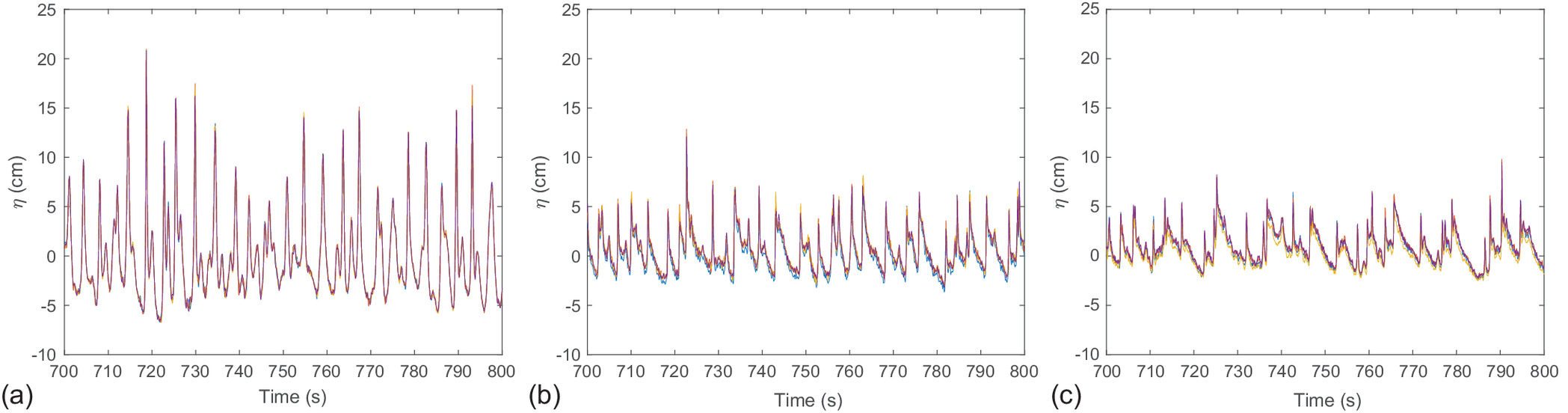
For each run, free-surface elevations were recorded simultaneously with an array of six resistive DHI wave gauges at 20 Hz mounted on a carriage. The absolute accuracy of these gauges is of nearly

\pm 1 mm

with a relative accuracy on the order of

\pm 0.2 mm

. The wave gauges were positioned every 1.0 m across the flume, from

x = - 22 m

to

x = 34 m

(Fig. 2). The repeatability of the experiments was assessed by maintaining a fixed probe 2 m shoreward of the wave paddle (

x = - 22 m

) for all runs, and several redundant measurements were performed at different locations during the experiment runs. In Fig. 3, four different runs of free surface measurements within the surf zone are shown. Only slight differences among runs are observed with an average absolute distance between signals of less than 6 mm; these differences may be explained by the randomness of the highly turbulent dynamics that exist within the surf zone.

Fig. 3. Free-surface measurements at different locations within the surf zone for four experimental runs: (a) $x = 14 m$ ; (b) $x = 30 m$ ; and (c) $x = 34 m$ .

These experiments were used to test the ability of the SGN equations to reproduce highly nonlinear wave dynamics, including wave–wave interactions and infragravity wave generation, propagation, and breaking dissipation.

Results

Capabilities of the Serre-Green-Naghdi Equations for Nonlinear Wave Interactions and Energy Transfers

The characteristic wavelength in the laboratory experiment was estimated from the linear theory using the swell peak frequency,

f_{p} = 0.25 Hz

, and the still-water depth in the horizontal part of the channel,

h_{0} = 0.52 m

, to be

λ_{h_{0}} = 8.84 m

; hence, the nondimensional parameters defined in Eqs. (1) and (2) are

ϵ_{h_{0}} = 0.346

,

δ_{h_{0}} = 0.059

,

U_{r, h_{0}} = 99.40

, and

Λ_{h_{0}} = 0.02

. These numbers show that the experimental high-frequency wave conditions are representative of a highly nonlinear shallow-water wave regime that is well beyond the range of validity of classical weakly dispersive and weakly nonlinear Boussinesq-type models relying on

U_{r} \sim O (1)

.

The experimental conditions are indeed very challenging and ideal to test the capabilities of the SGN equations to reproduce highly nonlinear wave processes in shallow waters. The corresponding Iribarren number (Galvin 1968; Battjes 1974)

I r_{b} = \frac{| ζ_{x} |}{\sqrt{H_{b} / λ_{0}}}

(15)

is estimated to be

I r_{b} = 0.16

, which is within the spilling breaking regime (

I r_{b} < 0.4

), thus ensuring the establishment of a wide surf zone in the laboratory beach. In Eq. (15),

H_{b}

is the characteristic wave height at the mean breaking position and

λ_{0}

is the equivalent wavelength in deep water. Wave height at breaking is estimated from measurements to be

H_{S, b} ≃ 0.15 m

(Fig. 4), while, based on the linear theory, the deep-water wavelength is

λ_{0} = 25 m

for the peak swell period; the beach slope is

| ζ_{x} | = 1 / 80

. The critical front wave angle to activate breaking terms in the SGN model is set to

θ_{b} = 25 °

, which is better for spilling breakers. This was expected because the default value of

θ_{b} = 30 °

reported in Cienfuegos et al. (2010a) was calibrated on regular wave experiments carried out over a much steeper beach slope (

| ζ_{x} | = 1 / 30

) with plunging breakers. The quadratic friction model of Eq. (13) was set with a friction coefficient

C_{f} = 0.001

. Sensitivity tests with friction coefficients in the range of

C_{f} = 0.001 - 0.005

were performed to choose this value, which gave the best results for the estimation of the swell and infragravity wave energy evolution within the surf zone (not shown).

Fig. 4. Wave heights computed from the power spectral density of free-surface time series. Plain lines = SGN model; symbols = experiment; circles = swell band [ $(3 / 5) f_{p} < f < 8 f_{p}$ ]; pluses = fundamental high-frequency harmonic ( $f_{p} - δ f < f < f_{p} + δ f$ ); crosses = second high-frequency harmonic ( $2 f_{p} - δ f < f < 2 f_{p} + δ f$ ); triangles = third high-frequency harmonic ( $3 f_{p} - δ f < f < 3 f_{p} + δ f$ ); and dashed line = infragravity band [ $(1 / 50) f_{p} < f < (3 / 5) f_{p}$ ].

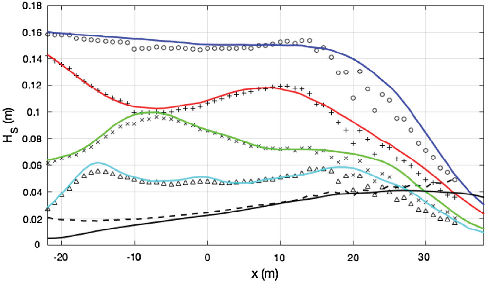
The spatial evolution of spectral wave energy and energy exchange among wave frequencies is presented in Fig. 4. Wave heights were estimated at each location from the power spectral density (PSD) of the free-surface time series integrated between specific frequency bands

H_{S} = 4 \sqrt{\int_{f_{1}}^{f_{2}} E (f) d f}

(16)

Wave heights were estimated for the swell band [

f_{1} = (3 / 5) f_{p}

,

f_{2} = 8 f_{p}

] and the infragravity band [

f_{1} = (1 / 50) f_{p}

,

f_{2} = (3 / 5) f_{p}

]; in addition, nonlinear interactions among high-frequency harmonics are depicted through wave heights integrated between

f_{1} = f_{p} - δ f

and

f_{2} = f_{p} + δ f

(first),

f_{1} = 2 f_{p} - δ f

and

f_{2} = 2 f_{p} + δ f

(second), and

f_{1} = 3 f_{p} - δ f

and

f_{2} = 3 f_{p} + δ f

(third), where

δ f = 0.125 Hz

. The agreement between measured and modeled wave heights is very good for all the studied frequency bands, though some discrepancies arise in the surf zone (

x > 15 m

). A slight underestimation of breaking energy dissipation is observed, which may explain the differences between measured and modeled high-frequency amplitudes within the surf zone. The energy exchange among high-frequency harmonics across the wave propagation process is striking, confirming the highly nonlinear regime of the experimental conditions. During the short-wave propagation over the horizontal part of the flume, energy transfer is observed, which is due to the resonant mechanism resulting from the interaction between forced and free harmonics (e.g., Mei 1989, Section 11.11).

The SGN model succeeds in reproducing these challenging nonlinear energy transfer dynamics, including the generation of ingragravity waves. Nonetheless, more infragravity energy is present in the experiment than in the numerical model. These differences are attributed to quasi-standing long waves that are present in the experimental flume owing to partial reflection on the wave paddle.

A linear modal analysis considering the flume configuration with a closed offshore wall gives

f_{n 1} = 0.013 Hz

,

f_{n 2} = 0.023 Hz

, and

f_{n 2} = 0.031 Hz

as the first, second, and third natural frequencies. In Fig. 5(a) the spectral signature of measured and modeled free-surface data at

x = - 22 m

(near the wave paddle) is presented: there is much more low-frequency energy in the experimental flume than in the model, with peaks around the natural frequencies. The spatial structure of significant wave heights integrated around these frequencies (taking

δ f = 0.003 Hz

) are shown in Fig. 5(b), thus confirming that the difference between measured and modeled infragravity wave energy is due to partial reflection of long waves at the paddle. Moreover, the experimental data follow the standing wave patterns for the natural modes, while the absorbing-generating boundary condition implemented in the SGN numerical model is transparent to infragravity waves reflected at the beach and propagating offshore.

Fig. 5. Analysis of natural modes of the wave flume: (a) spectral signature in the infragravity band estimated from experimental and numerical free surface data at $x = - 22 m$ . Experiment = dashed line; SGN model = plain line; and vertical thin dashed lines correspond to natural frequencies; and (b) spatial structure of significant wave heights integrated around natural frequencies. Experiment = black symbols; SGN = plain lines with symbols; circles = first mode $f_{n 1} = 0.013 Hz$ ; squares = second mode $f_{n 2} = 0.023 Hz$ ; and triangles = third mode $f_{n 3} = 0.031 Hz$ .

To further establish that the infragravity wave dynamics are not affected by the long-wave seiching in the experimental flume, we applied the time-domain incoming and outgoing wave separation method proposed by Almar et al. (2014) to low-pass filtered time series of experimental and modeled free-surface signals. We separated infragravity waves from short waves at each location using a low-pass filter with cutoff frequency

f_{c} = 3 / 5 f_{p}

applied on measured and computed free-surface time series. By doing so, we defined the high-frequency,

η_{hf} (x, t)

, and low-frequency,

η_{lf} (x, t)

, signal components at each location

x

. The incoming and outgoing wave separation method consists in applying the Radon transform (Deans 2007), which has been successfully implemented in surf zone wave applications by Almar et al. (2016), Martins et al. (2017), and Almar et al. (2017, 2018, 2021), among others. Here we closely follow the methodology described for a similar application in Martins et al. (2017) to separate the incoming and outgoing infragravity wave signals in the time domain to obtain

η_{lf} (x, t) = η_{lfin} (x, t) + η_{lfout} (x, t)

(17)

where

η_{lfin} (x, t)

and

η_{lfout} (x, t)

= incoming and outgoing infragravity wave signals at each location

x

, respectively.

The application of the method on experimental and numerical infragravity wave signals is shown in Fig. 6, where an excellent correspondence between the total time series and the ones obtained by summing up incoming and outgoing infragravity signals separated using the Radon transform is observed at the commencement of the beach slope (

x = 0 m

). The spatial evolution of incoming and outgoing infragravity wave signals estimated from the PSD [Eq. (16)] of the free-surface time series integrated between

f_{1} = (1 / 50) f_{p}

and

f_{2} = (3 / 5) f_{p}

is presented in Fig. 7. It is confirmed that the partial reflection on the wave paddle results in an increase of infragravity wave energy (in incoming and outgoing signals) in the experimental setup, but the latter mostly affects the long-wave dynamics outside of the surf zone (

x < 15 m

). Minor differences are observed within the surf zone between experimental and numerical data, thus giving confidence to the infragravity wave dynamics that are to be analyzed using the SGN model.

Fig. 6. Separation of incoming and outgoing infragravity wave signals using the Radon transform, illustrated for a wave gauge located at $x = 0 m$ : (a) incoming (blue) and outgoing (red) infragravity wave signals obtained from the experimental measurements; (b) total experimental infragravity wave signal (blue) and reconstructed time series summing up incoming and outgoing signals obtained by the Radon transform method applied to the experimental data (dashed black); (c) incoming (blue) and outgoing (red) infragravity wave signals obtained from the SGN model; and (d) total modeled infragravity wave signal (blue) and reconstructed time series summing up incoming and outgoing signals obtained by the Radon transform method applied to the modeled data (dashed black).

Fig. 7. Incoming (blue) and outgoing (red) infragravity wave heights computed from the PSD of the time signals obtained from the application of the Radon transform method described by Almar et al. (2016). Circles = experiments; and plain lines = SGN model.

To investigate the long-wave generation mechanisms responsible for the transfer of energy from the carrying narrow-band JONSWAP spectrum to the infragravity band, we present the cross-correlation analysis between the short-wave envelope and long waves following the procedure reported in Baldock and Huntley (2002) and Janssen et al. (2003), among others. To perform a correlation analysis between short-wave groups and infragravity waves, we define the high-frequency (hf)-wave envelope function using a Hilbert transform (e.g., Baldock and Huntley 2002)

| A (t) | = | η_{hf} (t) + i H {η_{hf} (t)} |

(18)

where

H {}

denotes de Hilbert transform; and

i

= pure imaginary number.

Long-wave generation and propagation are studied by means of a cross-correlation analysis between the short-wave envelope and long waves. We used the following normalized cross-correlation function (e.g., Bendat and Piersol 2011):

R_{p q} (τ) = \frac{⟨ p (t) q (t + τ) ⟩}{σ_{p} σ_{q}}

(19)

where

τ

= time shift;

⟨ ⟩

= time-averaging operator;

p (t)

and

q (t)

= two time series signals; and

σ_{p}

and

σ_{q}

= standard deviations of

p (t)

and

q (t)

respectively.

In Fig. 8, the cross-correlation function between the short-wave envelope measured at

x = - 22 m

and the infragravity frequency band computed at each location are presented for both the experimental [Fig. 8(a)] and the SGN model [Fig. 8(b)]. Very close to the wave paddle, the long waves are anticorrelated to the short-wave envelope as expected from the bound long-wave generation theory (e.g., Biesel 1952; Longuet-Higgins and Stewart 1962; Schäffer 1993). Nevertheless, a slight phase difference between the negative ridge and the carrying short-wave group is visible up to the inner surf zone, where the negative ridge disappears (

x \sim 22 - 25 m

). Janssen et al. (2003) observed a similar phase lag between the forced long-wave and the short-wave group in the shoaling process of their experimental conditions. The latter was confirmed and explained by Battjes et al. (2004), who demonstrated that this phase lag plays a fundamental role in the transfer of energy from the short waves to the bound long waves in the shoaling zone. In our experiment, the lag is noticed from the very beginning of the wave propagation owing to the highly nonlinear and shallow-water conditions of the incident short-wave field, implying nearly resonant conditions between forced and free long waves leading to the appearance of an N-shaped long-wave, with a positive surge ahead of the group, and a negative one lagging behind (Nielsen and Baldock 2010).

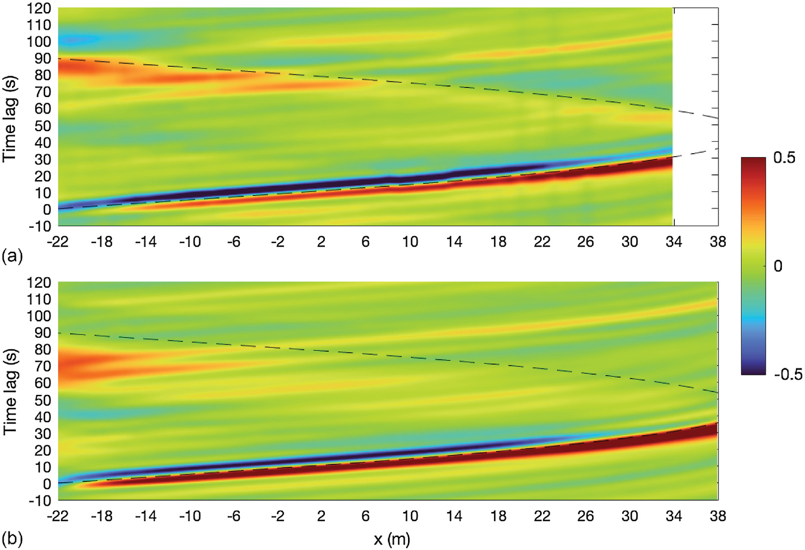
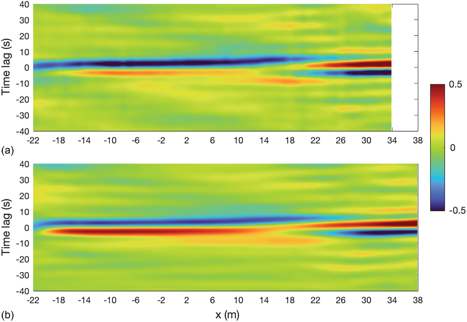
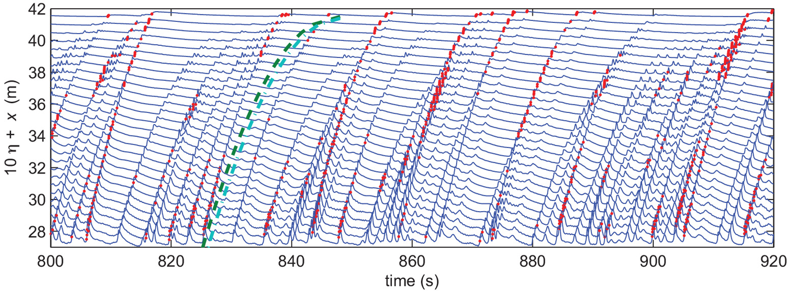
Fig. 8. Cross-correlation functions between the squared short-wave envelope, ${| A (t) |}^{2}$ , at $x = - 22 m$ , and the infragravity signal, $η_{lf} (t)$ , at the other locations: (a) experiment; and (b) SGN model. Dashed lines represent the incoming and reflected long-wave trajectories at the phase speed $c = \sqrt{g | ζ |}$ .

A closer inspection of the fate of the positive and negative ridges is made with the help of the cross-correlation map between the low-frequency surface elevation signals and the short-wave envelopes at identical positions as shown in Fig. 9. In the inner surf zone, there is a sudden shift in phase with the emergence of a positively correlated pulse at nearly zero time lag with the carrying short-wave group, and a negatively correlated ridge ahead of it. The latter is in agreement with results reported by van Dongeren et al. (2007) and Lara et al. (2011), who argued that in very shallow water, short-wave propagation is strongly influenced by low-frequency motions producing a convergence of short-wave fronts and long-wave bores; indeed, infragravity motions enhance nonlinear bore merging in the inner surf zone (Tissier et al. 2015). The latter is confirmed by the free-surface elevation time series plotted at consecutive locations within the inner surf zone in Fig. 10. In the inner surf zone, the merging of short waves is clearly observed, giving rise to bore-like long waves reaching the swash zone. The positive long-wave surge running ahead of the group experiences a rapid grow in amplitude and a nonlinear steepening in the surf zone due to the strong nonlinear interactions in very shallow waters between short waves and low-frequency motions. Similar patterns were observed on an experimental beach with the same slope in the Globex project (Ruessink et al. 2013).

Fig. 9. Cross-correlation function between the squared short-wave envelope ${| A (t) |}^{2}$ and the infragravity signal, $η_{lf} (t)$ , at the same locations: (a) experiment; and (b) SGN model.

Fig. 10. Time series of the free-surface elevation at consecutive locations within the inner surf zone computed by the SGN model. Red dots are used to mark breaking events using a front face’s wave angle threshold of 25°. The dashed and dash-dotted lines represent linear phase and group velocities respectively.

The agreement between SGN results and the measured features that arise from complex nonlinear wave–wave interactions, energy transfer among different wave frequencies, and infragravity wave dynamics is excellent. The SGN equations are thus the ideal depth-integrated set of equations to deal with strongly nonlinear and nonhydrostatic flows in shallow waters. The addition of a breaking dissipation model allows fair reproduction of the most important nonlinear processes within the surf and swash zones.

Bringing Together Coastal and Fluvial Hydraulics at the River Mouth: A Preliminary Exploration Based on the SGN Equations

Given the excellent performance that SGN equations have shown both in coastal and riverine research, it seems natural to move ahead to apply them to river mouth hydrodynamics, which is where the disciplines collide. Even if the depth-integrated essence of the model may obscure important physical processes, such as shear, vorticity, and mixing, it appears that SGN models would remain a powerful tool to describe first-order nonhydrostatic free-surface water wave dynamics, in particular for engineering applications (Kirby 2016; Castro-Orgaz and Hager 2019; Roy Biswas et al. 2021).

In this section we perform exploratory numerical experiments considering a simplified river mouth configuration. The latter is motivated by recent field work data showing that infragravity motions generated by surf zone wave processes, such as the ones described in the previous section, can penetrate upstream of shallow bar-built estuaries (e.g., Williams and Stacey 2016; Bertin et al. 2019; McSweeney et al. 2020; Brocchini 2020). We focus specifically on two features that have been described in these field observations: (1) wave blocking on the river outflow under certain conditions (e.g., Williams and Stacey 2016); and (2) energy transfers toward lower frequencies as infragravity waves are able to propagate upstream of the river mouth (e.g., McSweeney et al. 2020).

The simplified configuration of the river mouth is depicted in Fig. 11. The beach slope is 1/80 (offshore to the left), and the incident wave conditions are specified at

x = 0 m

where the still-water depth is

h_{0} = 10 m

. The river bed has a constant upstream slope of 5‰, and extends up to

x = 1,200 m

, where the river discharge is specified. At

x = 640 m

, we define a bar with an offshore slope of 4/100, a bar crest length of 10 m at a vertical elevation of

z = 0 m

, and a slope of 2/100 toward the river. In Fig. 11 the location of the river mouth is depicted in vertical dashed lines at

x = 700 m

.

Fig. 11. Simplified bathymetric configuration for the numerical experiments and free-surface snapshots for different offshore sea levels. The vertical dashed lines show the location of the river mouth at $x = 700 m$ . Black line = bathymetry; blue line = snapshot of the free surface at $t = 1,550 s$ (waves start entering at the left boundary of the domain when $t = 0 s$ ); blue dash-dotted line = time-averaged free surface; red line = time-averaged depth-averaged velocities; and red dashed line = time-averaged Froude number.

The incoming discharge from the river is kept constant,

Q = 0.8 m^{2} / s

, and a 60-min time series wave signal, obtained from a JONSWAP spectrum with a significant wave height

H_{m 0} = 2.0 m

, a peak frequency

f_{p} = 0.0833 Hz

, a peak enhancement factor 3.3 (Goda 2000), and a random phase distribution, is specified at the offshore boundary. In the computations, we use a Manning friction coefficient

n = 0.025

and set the parameters of the breaking dissipation model to their default values (Cienfuegos et al. 2010a). The characteristic wavelength is estimated to be

λ_{h_{0}} = 224.8 m

from the linear theory using the swell peak frequency,

f_{p} = 0.0833 Hz

and the water depth

h_{0} = 10 m

; hence, the nondimensional parameters are

ϵ_{h_{0}} = 0.2

,

δ_{h_{0}} = 0.0445

,

U_{r, h_{0}} = 101.10

, and

Λ_{h_{0}} = 0.009

. The Ursell number is similar to the one reported in the experimental conditions of the previous section, typical of a highly nonlinear shallow-water wave regime.

Before allowing the offshore waves to enter the domain, we ran the model until a steady-state equilibrium for the river flowing downstream was reached; the Froude number associated to the uniform flow upstreams is

F_{r} = 0.71

. In the numerical experiments, the only variable that we changed was the offshore sea level, so different Froude numbers at the river mouth could be set. For runs that include waves entering the domain, the Froude number was computed as the time average over the simulations

\bar{F_{r}} (x) = \frac{1}{Δ t} \int_{t_{0}}^{t_{0} + Δ t} \frac{| u (x, t) |}{\sqrt{g (η (x, t) - ζ (x))}} d t

(20)

where

t_{0} = 480 s

to allow the wave regime to be established (

\sim 40

waves); and

Δ t = 3,120 s

. Similarly, we define the time average of depth-averaged velocities as

\bar{u} (x) = \frac{1}{Δ t} \int_{t_{0}}^{t_{0} + Δ t} u (x, t) d t

(21)

A remarkable feature of the SGN model in the context of hydraulic engineering practice is its ability to deal with nonhydrostatic shallow-water flows. The fluid pressure at the bottom of the water column may be estimated along the channel as (Seabra-Santos et al. 1987; Cienfuegos 2005)

P_{b} (x, t) = ρ g (η (x, t) - ζ (x)) + ρ \int_{ζ}^{η} Γ (x, z, t) d z

(22)

where the first term is the hydrostatic contribution; the second is the nonhydrostatic part; and

Γ (x, z, t)

= vertical acceleration of the fluid that may be expressed in terms of the depth-averaged horizontal velocity and its derivatives [truncating terms of

O (δ^{4})

] as

Γ (x, z, t) = \frac{(z - ζ)}{(η - ζ)} P (x, t) + Q (x, t)

(23)

where

P (x, t) = - (η - ζ) (u_{x t} + u u_{x x} - u_{x}^{2})

(24)

Q (x, t) = ζ_{x} (u_{t} + u u_{x}) + ζ_{x x} u^{2}

(25)

With these definitions, the bottom piezometric head of the fluid reads

H_{b} = ζ + \frac{P_{b} (x, t)}{ρ g} = η (x, t) + \frac{1}{g} (η (x, t) - ζ (x)) (\frac{1}{2} P (x, t) + Q (x, t))

(26)

where the second term on the right-hand side corresponds to the nonhydrostatic contribution.

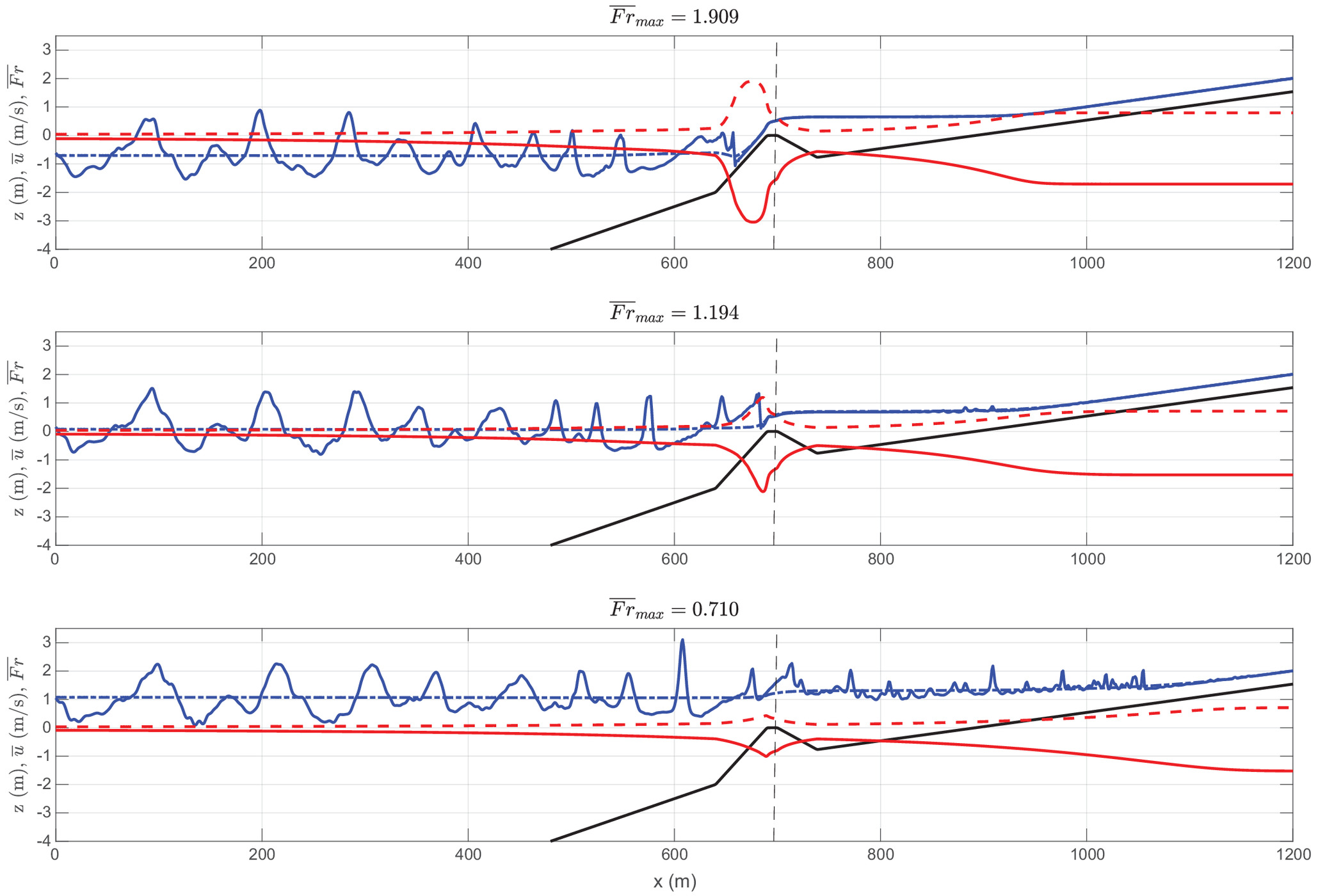
In Fig. 11, snapshots of the free surface at

t = 1,550 s

are shown for different sea levels, resulting in different time-averaged Froude numbers and depth-averaged velocities. Supercritical, nearly critical, and subcritical flow conditions over the bar are shown with maximum time-averaged values of

{\bar{F r}}_{\max} = 1.909

,

{\bar{F r}}_{\max} = 1.194

, and

{\bar{F r}}_{\max} = 0.710

, respectively. The results confirm that a blocking of the incoming offshore waves occurs under supercritical conditions, as observed in the field when the “estuarine mouth is perched above the low tide ocean water level” (Williams and Stacey 2016).

The free surface and the bottom piezometric head are shown for the case with

{\bar{F r}}_{\max} = 0.710

in Fig. 12. The differences between the variables are more pronounced where the free surface curvatures are stronger. In general, the bottom piezometric head tends to be below the free surface under narrow wave crests, and the opposite occurs near the wave troughs.

Fig. 12. Snapshots of free surface (blue) and bottom piezometric head (red) for the case with ${\bar{F r}}_{\max} = 0.710$ at $t = 1,550 s$ . The vertical dashed line shows the location of the river mouth at $x = 700 m$ , and the black line shows the location of the bathymetry.

Fig. 13 presents the spatial evolution of wave heights computed from the PSD [Eq. (16)] integrated between

f_{1} = (3 / 5) f_{p}

and

f_{2} = 8 f_{p}

(swell energy band), and between

f_{1} = (1 / 50) f_{p}

and

f_{2} = (3 / 5) f_{p}

(infragravity energy band). There is a rapid decay of the swell wave heights near the offshore side of the bar (

600 < x < 700

), while the infragravity wave energy increases in the same zone. For the higher supercritical Froude numbers over the bar (1.909 and 1.713), the infragravity energy grows rapidly and exceeds the swell energy before reaching the bar; very little wave energy (swell or infragravity) penetrates upstream under these Froude numbers. For the remaining simulations (Froude numbers of 1.194, 0.777, 0.712, and 0.710), wave energy is capable of propagating upstream of the bar, penetrating farther when the Froude number is lower. The spectral wave energy appears to be nearly equally partitioned between the swell and infragravity bands while propagating through the river. Nevertheless, it appears that the Fourier analysis would no longer be useful to characterize the strongly nonlinear wave dynamics the

x - t

maps suggest in Fig. 14. Indeed, recent studies have demonstrated that standard linear Fourier analysis fails in revealing the hidden soliton dynamics in long-wave bore propagation (Brühl et al. 2022).

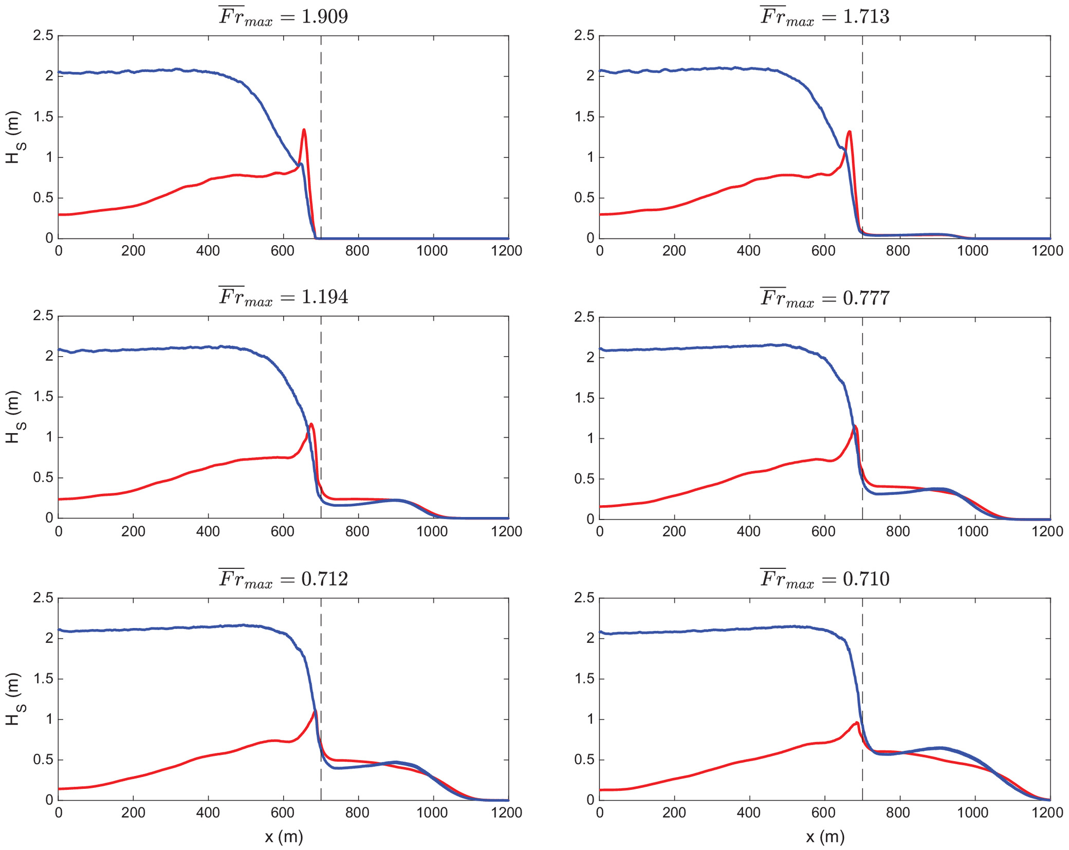
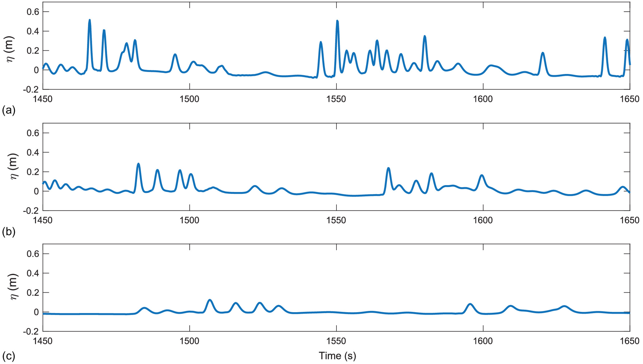
Fig. 13. Wave heights computed from the power spectral density of the free-surface time series. Blue line = swell band [ $(3 / 5) f_{p} < f < 8 f_{p}$ ]; red line = infragravity band [ $(1 / 50) f_{p} < f < (3 / 5) f_{p}$ ]. The vertical dashed lines show the location of the river mouth at $x = 700 m$ .

Fig. 14. Time stacks of free-surface time series along the simplified river mouth configuration for different Froude numbers above the bar. The vertical dashed lines show the location of the river mouth at $x = 700 m$ .

The timestacks of free-surface time series presented in Fig. 14 highlight the importance of the river mouth Froude number in controlling the infragravity wave propagation into the river, a feature that has been described as a low-pass filtering property of shallow bar-built river inlets (e.g., Williams and Stacey 2016; Bertin et al. 2019; Melito et al. 2020; McSweeney et al. 2020). When the Froude number is high enough, neither short nor infragravity waves can propagate upstream [Figs. 14(a and b)]. As the Froude numbers decrease, approaching critical (

\sim 1

) and for subcritical conditions (

< 1

), some waves are able to penetrate and propagate upstream. The strongly nonlinear propagation of individual waves is remarkable because either merging or separating trajectories can be observed. A closer view of the evolution of the free-surface time series at

x = 1,000 m

,

x = 1,030 m

, and

x = 1,060 m

for the Froude number 0.712 over the bar is presented in Fig. 15. Waves propagating upstream are organized as wave packets, which appear to result from the fission of long waves into solitons, a feature that has been documented in tsunami-like propagating upstream rivers (Tsuji et al. 1991), and over mild slope bathymetries (e.g., Matsuyama et al. 2007).

Fig. 15. Free-surface time series at different spatial positions within the river for a Froude number 0.712 over the bar: (a) $x = 1,000 m$ ; (b) $x = 1,030 m$ ; and (c) $x = 1,060 m$ .

These wave packets giving rise to solitonic dynamics have also been observed in field measurements of wind wave propagation in Currituck Sound, North Carolina, over a shallow flat area with depths in the range of 1.8–2.4 m by Long and Resio (2007). By analyzing the same data set using linear Fourier transform, Costa et al. (2014) established that the infragravity range dominated by solitonic dynamics had a power spectral signature of

\sim f^{- 1}

. Fig. 16 shows the PSD of free surface time series between

x = 640 m

(the offshore toe of the bar) and

x = 900 m

(upstream of the river mouth), evenly spaced between

Δ x = 10 m

. It is seen that while propagating over the bar, the infragravity PSD signature has a slope

\sim f^{- 1}

, thus consistent with the observations of solitonic dynamics in low-frequency bands made by Costa et al. (2014). The latter supports the soliton fission mechanism described previously; nonlinear Fourier transforms would be necessary to adequately analyze these dynamics as discussed in Brühl et al. (2022).

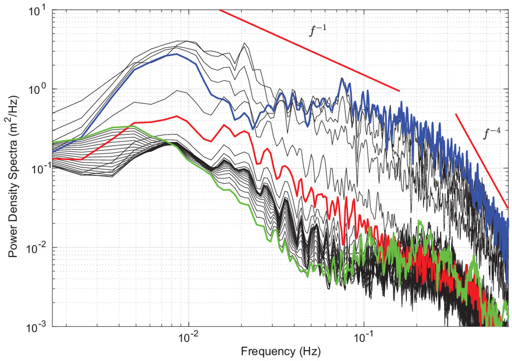
Fig. 16. PSD signatures for free-surface time series between $x = 640$ and $x = 900 m$ , evenly spaced every $Δ x = 10 m$ , computed for the case ${\bar{F r}}_{\max} = 1.194$ . Blue = PSD computed from the wave gauge located at $x = 640 m$ ; red = PSD computed from the wave gauge located at $x = 700 m$ ; green = PSD computed from the wave gauge located at $x = 900 m$ . $f^{- 1}$ and $f^{- 4}$ slopes are shown for reference in red.

Fig. 17 plots the cross-correlation functions between the short-wave envelope at

x = 0 m

and the long-wave signal at other locations for the simulations with Froude numbers of 1.909 [Fig. 17(a)], 1.194 [Fig. 17(b)], and 0.710 [Fig. 17(c)]. In the surf zone, the pattern of the incoming infragravity waves is similar to the one presented in Fig. 8, with a positive surge ahead of the group and a negative one lagging behind it; but there are important differences regarding the long-wave energy that is reflected offshore. For a Froude number of 1.909, the blocking of waves at the river mouth is clear, while strong dissipation and reflection of long waves appears to take place near the bar. As the Froude number decreases, the positive surge is able to penetrate the river. The latter is very clear for the Froude number of 0.710, where the signal of the positive surge advancing upstream is very strong, while the negatively correlated signal is much weaker.

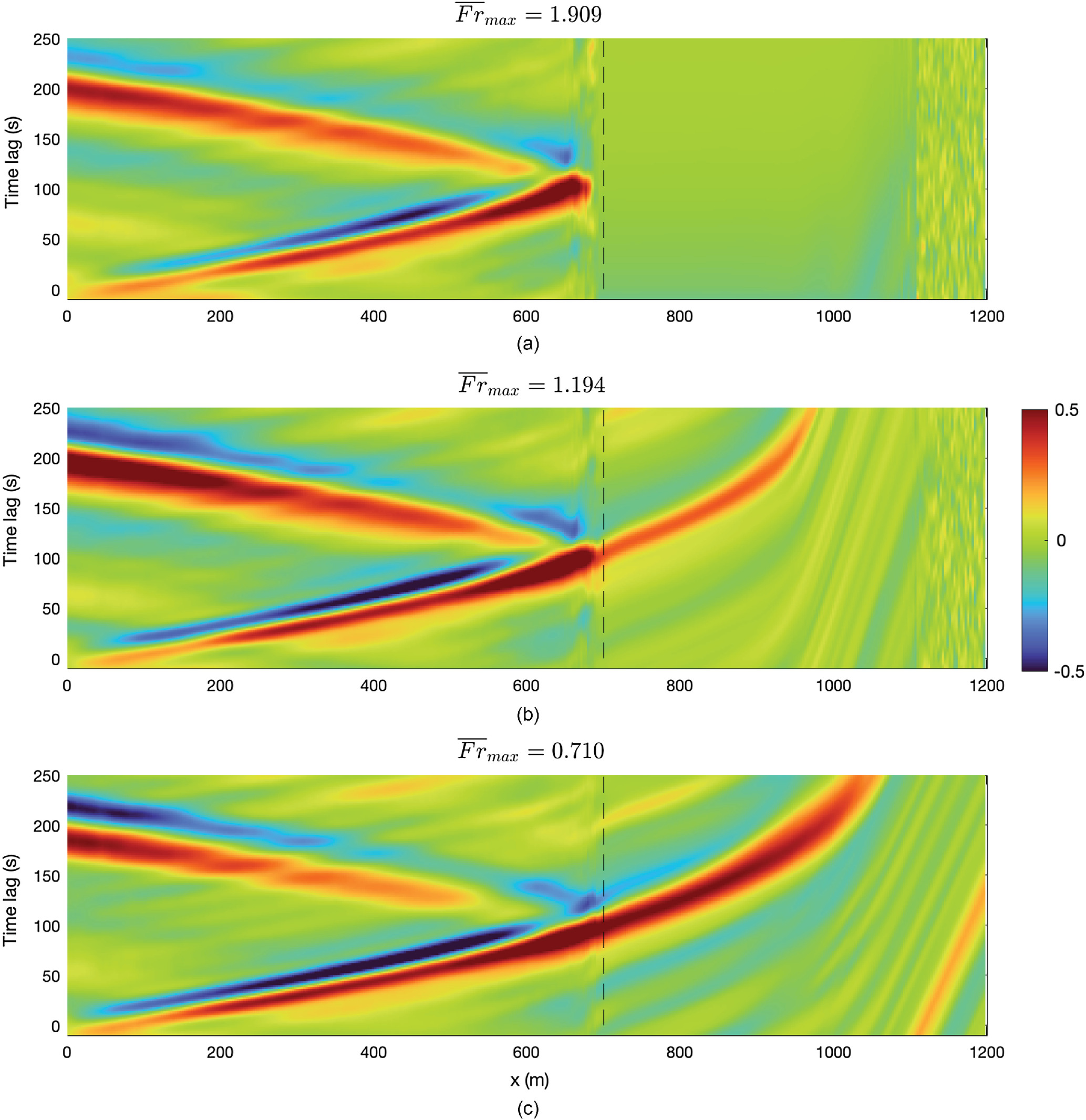
Fig. 17. Cross-correlation functions between the squared short-wave envelope, ${| A (t) |}^{2}$ , at $x = 0 m$ , and the infragravity signal, $η_{lf} (t)$ , at the other locations. The vertical dashed lines show the location of the river mouth at $x = 700 m$ .

By comparing the cross-correlation maps for the experimental surf zone shown in Fig. 8 and for the infragravity waves propagating in the numerical river mouth configuration presented in Fig. 17, we conclude that the generation mechanism for the infragravity waves in both cases is the same, but much higher long-wave energy is reflected offshore in the bar-built shallow-estuary configuration. Moreover, Fig. 15 suggests a similar behavior for convergent bore-like long waves propagating upstream the river, and a fission of these nonlinear fronts into solitons as depicted in Fig. 15. As shown previously, the PSD signature of the free-surface time series supports the latter. On the other hand, by comparing the PSD evolution between

x = 640 m

(offshore toe of the bar),

x = 700 m

(bar location), and

x = 900 m

(upstream of the bar) in Fig. 16, a transfer of energy into lower frequencies is observed, similar to the one described in the field data of McSweeney et al. (2020). Nevertheless, an inverse energy cascade from the infragravity band back to the swell energy band is also present. The standard linear Fourier analysis in the frequency domain is not able to see the solitonic dynamic that is in place, and the frequency separation between infragravity and swell energy bands would no longer be adequate, so nonlinear frameworks for wave analysis should be employed to elucidate the fate of these long waves, as discussed previously.

Conclusions

The SGN equations constitute a powerful tool to model fully nonlinear and weakly dispersive wave processes in the shoaling, surf, and swash zones if appropriate breaking dissipation parameterizations are incorporated. They are able to fairly reproduce the complexities of wave–wave interactions and nonlinear frequency transfers from a narrow-band wave spectrum into higher and lower frequencies. In particular, infragravity wave generation, propagation, and swash zone dynamics are well captured. The latter is demonstrated by testing the numerical model used in this work on challenging experimental conditions run on a wave flume.

Moreover, SGN equations are also capable of reproducing riverine flows and transients generated by the sudden operation of weirs and gates, and, more generally, open-channel flows with nonnegligible vertical accelerations by dropping the hydrostatic pressure distribution assumption. The latter is of particular interest for expanding the limits of traditional hydraulic modeling, and would also deserve more attention in teaching and research practice within this discipline. We have thus explored in this work the application of the set of SGN equations to surf zone processes involving infragravity wave generation and their penetration into river mouths. We have studied, through numerical experiments, the fate of infragravity waves on a simplified shallow bar-built estuary with constant river discharge and different sea levels. The simulations confirm that a blocking of the incoming offshore waves occurs under supercritical conditions over the bar, as previously observed in several field campaigns. Infragravity waves start penetrating upstream when the Froude number approaches and falls below 1. When long waves are able to penetrate, they experience a strongly nonlinear propagation, where both merging and separating individual trajectories are observed. It appears that they propagate upstream as wave packets that may result from the fission of long waves into solitons. The PSD signatures of free-surface time series at different locations from offshore of the bar toward the river support the latter because a

\sim f^{- 1}

slope is observed in the PSD, consistent with previous field observations of solitonic dynamics in coastal waves. The numerical experiments performed here show a transfer of energy toward lower frequencies while the long waves propagate upstream of the river mouth, as suggested by recent field data; however, low-frequency energy is also able to cascade back to the high-frequency swell band. Nonlinear signal analysis techniques should be employed to confirm and characterize these complex energy transfers.

Data Availability Statement

The experimental and numerical data reported in this article are accessible by request to the author.

Acknowledgments

The reported surf zone wave experiment was conducted in the facilities of the Instituto Nacional de Hidráulica (INH) in Chile; I am grateful for all the technical support the INH staff provided during the study. The work done by Maricarmen Guerra and Leonardo Duarte in the laboratory during the undergraduate project of Leonardo is to be commended and recognized. I also acknowledge discussions and exchanges that have taken place over the years on infragravity waves with Professor Eric Barthélemy and Dr. Hervé Michallet from the Laboratoire des Écoulements Géphysiques et Industriels (LEGI) in Grenoble, France, and with Dr. Rafael Almar from the Laboratoire d’Études en Géophysique et Océanographie Spatiales (LEGOS) in Toulouse, France. I also acknowledge the careful reviews and constructive suggestions made by the two anonymous reviewers, and the associated and chief journal editors. This work has been partially funded by the Centro de Investigación para la Gestión Integrada del Riesgo de Desastres (CIGIDEN), through the grant ANID/FONDAP/1522A0005 and by the ANID/FONDEF/ID22I10087 project.

References

Airy, G. 1841. “Tides and waves.” In Encyclopaedia metropolitana (1817–1845), mixed sciences, 3. London: Hugh James Rose Eds.

Google Scholar

Almar, R., et al. 2021. “Sea state from single optical images: A methodology to derive wind-generated ocean waves from cameras, drones and satellites.” Remote Sens. 13 (4): 679. https://doi.org/10.3390/rs13040679.

Google Scholar

Almar, R., C. Blenkinsopp, L. P. Almeida, R. Cienfuegos, and P. A. Catalan. 2017. “Wave runup video motion detection using the radon transform.” Coastal Eng. 130 (Dec): 46–51. https://doi.org/10.1016/j.coastaleng.2017.09.015.

Google Scholar

Almar, R., S. Larnier, B. Castelle, T. Scott, and F. Floc’h. 2016. “On the use of the radon transform to estimate longshore currents from video imagery.” Coastal Eng. 114 (Aug): 301–308. https://doi.org/10.1016/j.coastaleng.2016.04.016.

Google Scholar

Almar, R., H. Michallet, R. Cienfuegos, P. Bonneton, M. Tissier, and G. Ruessink. 2014. “On the use of the radon transform in studying nearshore wave dynamics.” Coastal Eng. 92 (Oct): 24–30. https://doi.org/10.1016/j.coastaleng.2014.06.008.

Google Scholar

Almar, R., A. Nicolae Lerma, B. Castelle, and T. Scott. 2018. “On the influence of reflection over a rhythmic swash zone on surf zone dynamics.” Ocean Dyn. 68 (7): 899–909. https://doi.org/10.1007/s10236-018-1165-5.

Google Scholar

Arcement, G. J., and V. R. Schneider. 1989. Guide for selecting manning’s roughness coefficients for natural channels and flood plains. Denver: USGS.

Google Scholar

Baldock, T., and D. Huntley. 2002. “Long-wave forcing by the breaking of random gravity waves on a beach.” Proc. R. Soc. London, Ser. A 458 (2025): 2177–2201. https://doi.org/10.1098/rspa.2002.0962.

Google Scholar

Barré de Saint-Vénant, A. J.-C. 1871. “Théorie du mouvement non-permanent des eaux, avec application aux crues des rivières et à l’introduction des marées dans leur lit.” C. R. Acad. Sci. Paris 73 (147–154): 237–240.

Google Scholar

Barthélemy, E. 2004. “Nonlinear shallow water theories for coastal waves.” Surv. Geophys. 25 (3): 315–337. https://doi.org/10.1007/s10712-003-1281-7.

Google Scholar

Battjes, J. 1974. “Surf similarity.” In Coastal engineering, 26–26. Reston, VA: ASCE.

Google Scholar

Battjes, J., H. Bakkenes, T. Janssen, and A. R. van Dongeren. 2004. “Shoaling of subharmonic gravity waves.” J. Geophys. Res.: Oceans 109 (C2). https://doi.org/10.1029/2003JC001863.

Google Scholar

Bendat, J. S., and A. G. Piersol. 2011. Random data: Analysis and measurement procedures. Hoboken, NJ: Wiley.

Google Scholar

Bertin, X., D. Mendes, K. Martins, A. B. Fortunato, and L. Lavaud. 2019. “The closure of a shallow tidal inlet promoted by infragravity waves.” Geophys. Res. Lett. 46 (12): 6804–6810. https://doi.org/10.1029/2019GL083527.

Google Scholar

Biesel, F. 1952. “Équations générales au second ordre de la houle irrégulière.” Houille Blanche 3 (3): 372–376. https://doi/abs/10.1051/lhb/1952033.

Google Scholar

Bonneton, P., E. Barthelemy, F. Chazel, R. Cienfuegos, D. Lannes, F. Marche, and M. Tissier. 2011. “Recent advances in Serre–Green Naghdi modelling for wave transformation, breaking and runup processes.” Eur. J. Mech. B. Fluids 30 (6): 589–597. https://doi.org/10.1016/j.euromechflu.2011.02.005.

Google Scholar

Boussinesq, J. 1872. “Théorie des ondes et des remous qui se propagent le long d’un canal rectangulaire horizontal, en communiquant au liquide contenu dans ce canal des vitesses sensiblement pareilles de la surface au fond.” J. Math. Pures Appl. 17: 55–108.

Google Scholar

Briganti, R., R. Musumeci, G. Bellotti, M. Brocchini, and E. Foti. 2004. “Boussinesq modeling of breaking waves: Description of turbulence.” J. Geophys. Res.: Oceans 109 (C7). https://doi.org/10.1029/2003JC002065.

Google Scholar

Brocchini, M. 2013. “A reasoned overview on boussinesq-type models: The interplay between physics, mathematics and numeric.” Proc. R. Soc. London, Ser. A 469 (2160): 20130496. https://doi.org/10.1098/rspa.2013.0496.

Google Scholar

Brocchini, M. 2020. “Wave-forced dynamics in the nearshore river mouths, and swash zones.” Earth Surf. Processes Landforms 45 (1): 75–95. https://doi.org/10.1002/esp.4699.

Google Scholar

Brühl, M., P. J. Prins, S. Ujvary, I. Barranco, S. Wahls, and P. L.-F. Liu. 2022. “Comparative analysis of bore propagation over long distances using conventional linear and KdV-based nonlinear Fourier transform.” Wave Motion 111 (May): 102905. https://doi.org/10.1016/j.wavemoti.2022.102905.

Google Scholar

Cantero-Chinchilla, F. N., O. Castro-Orgaz, S. Dey, and J. L. Ayuso. 2016. “Nonhydrostatic dam break flows. I: Physical equations and numerical schemes.” J. Hydraul. Eng. 142 (12): 04016068. https://doi.org/10.1061/(ASCE)HY.1943-7900.0001205.

Google Scholar

Castro-Orgaz, O., and W. H. Hager. 2019. Shallow water hydraulics. Berlin: Springer.

Crossref

Google Scholar

Church, J. C., and E. B. Thornton. 1993. “Effects of breaking wave induced turbulence within a longshore current model.” Coastal Eng. 20 (1–2): 1–28. https://doi.org/10.1016/0378-3839(93)90053-B.

Google Scholar

Cienfuegos, R., E. Barthélemy, and P. Bonneton. 2006. “A fourth-order compact finite volume scheme for fully nonlinear and weakly dispersive Boussinesq-type equations. Part I: Model development and analysis.” Int. J. Numer. Methods Fluids 51 (11): 1217–1253. https://doi.org/10.1002/fld.1141.

Google Scholar

Cienfuegos, R., E. Barthélemy, and P. Bonneton. 2007. “A fourth-order compact finite volume scheme for fully nonlinear and weakly dispersive Boussinesq-type equations. Part II: Boundary conditions and validation.” Int. J. Numer. Methods Fluids 53 (9): 1423–1455. https://doi.org/10.1002/fld.1359.

Google Scholar

Cienfuegos, R., E. Barthélemy, and P. Bonneton. 2010a. “Wave-breaking model for Boussinesq-type equations including roller effects in the mass conservation equation.” J. Waterw. Port Coastal Ocean Eng. 136 (1): 10–26. https://doi.org/10.1061/(ASCE)WW.1943-5460.0000022.

Google Scholar

Cienfuegos, R., L. Duarte, L. Suarez, and P. Catalán. 2010b. “Numerical computation of infragravity wave dynamics and velocity profiles using a fully nonlinear Boussinesq model.” Coastal Eng. Proc. 1 (32): 48. https://doi.org/10.9753/icce.v32.currents.48.

Google Scholar

Cienfuegos, R. A. 2005. “Modélisation numérique des houles bidimensionnelles et du déferlement bathymétrique.” Ph.D. thesis, Terre, Univers, Environnement, Institut National Polytechnique de Grenoble, France.

Google Scholar

Costa, A., A. R. Osborne, D. T. Resio, S. Alessio, E. Chrivì, E. Saggese, K. Bellomo, and C. E. Long. 2014. “Soliton turbulence in shallow water ocean surface waves.” Phys. Rev. Lett. 113 (10): 108501. https://doi.org/10.1103/PhysRevLett.113.108501.

Google Scholar

Deans, S. R. 2007. The radon transform and some of its applications. Mineaola, NY: Dover Publications.

Google Scholar

Galvin, C. J. 1968. “Breaker type classification on three laboratory beaches.” J. Geophys. Res. 73 (12): 3651–3659. https://doi.org/10.1029/JB073i012p03651.

Google Scholar

Goda, Y. 2000. Random seas and design of maritime structures. 2nd ed. Singapore: World Scientific.

Crossref

Google Scholar

Grant, W. D., and O. S. Madsen. 1979. “Combined wave and current interaction with a rough bottom.” J. Geophys. Res.: Oceans 84 (C4): 1797–1808. https://doi.org/10.1029/JC084iC04p01797.

Google Scholar

Green, A. E., and P. M. Naghdi. 1976. “A derivation of equations for wave propagation in water of variable depth.” J. Fluid Mech. 78 (2): 237–246. https://doi.org/10.1017/S0022112076002425.

Google Scholar

Janssen, T., J. Battjes, and A. Van Dongeren. 2003. “Long waves induced by short-wave groups over a sloping bottom.” J. Geophys. Res.: Oceans 108 (C8): 1–14. https://doi.org/10.1029/2002JC001515.

Google Scholar

Julien, P. Y. 2010. Erosion and sedimentation. Cambridge, UK: Cambridge University Press.

Crossref

Google Scholar

Kennedy, A. B., Q. Chen, J. T. Kirby, and R. A. Dalrymple. 2000. “Boussinesq modeling of wave transformation, breaking, and runup. I: 1D.” J. Waterw. Port Coastal Ocean Eng. 126 (1): 39–47. https://doi.org/10.1061/(ASCE)0733-950X(2000)126:1(39).

Google Scholar

Kim, D.-H. 2015. “H2D morphodynamic model considering wave, current and sediment interaction.” Coastal Eng. 95 (Jan): 20–34. https://doi.org/10.1016/j.coastaleng.2014.09.006.

Google Scholar

Kim, D.-H., and P. J. Lynett. 2011. “Turbulent mixing and passive scalar transport in shallow flows.” Phys. Fluids (1994) 23 (1): 016603. https://doi.org/10.1063/1.3531716.

Google Scholar

Kirby, J. T. 2016. “Boussinesq models and their application to coastal processes across a wide range of scales.” J. Waterw. Port Coastal Ocean Eng. 142 (6): 03116005. https://doi.org/10.1061/(ASCE)WW.1943-5460.0000350.

Google Scholar

Korteweg, D. J., and G. de Vries. 1895. “On the change of form of long waves advancing in a rectangular canal, and on a new type of long stationary waves.” London Edinburgh Dublin Philos. Mag. J. Sci. 39 (240): 422–443. https://doi.org/10.1080/14786449508620739.

Google Scholar

Lara, J. L., A. Ruju, and I. J. Losada. 2011. “Reynolds averaged Navier–Stokes modelling of long waves induced by a transient wave group on a beach.” Proc. R. Soc. London, Ser. A 467 (2129): 1215–1242. https://doi.org/10.1098/rspa.2010.0331.

Google Scholar

Long, C. E., and D. T. Resio. 2007. “Wind wave spectral observations in Currituck Sound, North Carolina.” J. Geophys. Res.: Oceans 112 (C5). https://doi.org/10.1029/2006JC003835.

Google Scholar

Longuet-Higgins, M. S., and R. Stewart. 1962. “Radiation stress and mass transport in gravity waves, with application to ‘surf beats.’” J. Fluid Mech. 13 (4): 481–504. https://doi.org/10.1017/S0022112062000877.

Google Scholar

Martins, K., C. E. Blenkinsopp, R. Almar, and J. Zang. 2017. “The influence of swash-based reflection on surf zone hydrodynamics: A wave-by-wave approach.” Coastal Eng. 122 (Apr): 27–43. https://doi.org/10.1016/j.coastaleng.2017.01.006.

Google Scholar

Matsuyama, M., M. Ikeno, T. Sakakiyama, and T. Takeda. 2007. “A study of tsunami wave fission in an undistorted experiment.” In Tsunami and its hazards in the Indian and pacific oceans, 617–631. Basel, Switzerland: Springer.

Crossref

Google Scholar

McSweeney, S. L., J. C. Stout, and D. M. Kennedy. 2020. “Variability in infragravity wave processes during estuary artificial entrance openings.” Earth Surf. Processes Landforms 45 (13): 3414–3428. https://doi.org/10.1002/esp.4974.

Google Scholar

Mei, C. C. 1989. Vol. 1 of The applied dynamics of ocean surface waves. Singapore: World Scientific.

Google Scholar

Melito, L., M. Postacchini, A. Sheremet, J. Calantoni, G. Zitti, G. Darvini, P. Penna, and M. Brocchini. 2020. “Hydrodynamics at a microtidal inlet: Analysis of propagation of the main wave components.” Estuarine Coastal Shelf Sci. 235 (Apr): 106603. https://doi.org/10.1016/j.ecss.2020.106603.

Google Scholar

Michallet, H., R. Cienfuegos, E. Barthélemy, and F. Grasso. 2011. “Kinematics of waves propagating and breaking on a barred beach.” Eur. J. Mech. B. Fluids 30 (6): 624–634. https://doi.org/10.1016/j.euromechflu.2010.12.004.

Google Scholar

Mignot, E., and R. Cienfuegos. 2009. “On the application of a Boussinesq model to river flows including shocks.” Coastal Eng. 56 (1): 23–31. https://doi.org/10.1016/j.coastaleng.2008.06.007.

Google Scholar

Mohapatra, P. K., and M. H. Chaudhry. 2004. “Numerical solution of Boussinesq equations to simulate dam-break flows.” J. Hydraul. Eng. 130 (2): 156–159. https://doi.org/10.1061/(ASCE)0733-9429(2004)130:2(156).

Google Scholar

Moris, J. P., P. A. Catalán, and R. Cienfuegos. 2021. “Incorporating wave-breaking data in the calibration of a Boussinesq-type wave model.” Coastal Eng. 168 (Sep): 103945. https://doi.org/10.1016/j.coastaleng.2021.103945.

Google Scholar

Musumeci, R. E., I. A. Svendsen, and J. Veeramony. 2005. “The flow in the surf zone: A fully nonlinear Boussinesq-type of approach.” Coastal Eng. 52 (7): 565–598. https://doi.org/10.1016/j.coastaleng.2005.02.007.

Google Scholar

Nadiga, B., L. Margolin, and P. Smolarkiewicz. 1996. “Different approximations of shallow fluid flow over an obstacle.” Phys. Fluids (1994) 8 (8): 2066–2077. https://doi.org/10.1063/1.869009.

Google Scholar

Nielsen, P., and T. E. Baldock. 2010. “И-shaped surf beat understood in terms of transient forced long waves.” Coastal Eng. 57 (1): 71–73. https://doi.org/10.1016/j.coastaleng.2009.09.003.

Google Scholar

Peregrine, D. H. 1967. “Long waves on a beach.” J. Fluid Mech. 27 (4): 815–827. https://doi.org/10.1017/S0022112067002605.

Google Scholar

Roy Biswas, T., S. Dey, and D. Sen. 2021. “Modeling positive surge propagation in open channels using the Serre-Green-Naghdi equations.” Appl. Math. Modell. 97 (Sep): 803–820. https://doi.org/10.1016/j.apm.2021.04.028.

Google Scholar

Ruessink, B. G., H. Michallet, P. Bonneton, D. Mouazé, J. Lara, P. A. Silva, and P. Wellens. 2013. “Globex: Wave dynamics on a gently sloping laboraty beach.” In Proc., Coastal Dynamics 2013, 1351–1362. Utrecht, Netherlands: Utrecht Univ. Repository.

Google Scholar

Schäffer, H. A. 1993. “Infragravity waves induced by short-wave groups.” J. Fluid Mech. 247 (Feb): 551–588. https://doi.org/10.1017/S0022112093000564.

Google Scholar

Schäffer, H. A. 1996. “Second-order wavemaker theory for irregular waves.” Ocean Eng. 23 (1): 47–88. https://doi.org/10.1016/0029-8018(95)00013-B.

Google Scholar

Schäffer, H. A., P. A. Madsen, and R. Deigaard. 1993. “A Boussinesq model for waves breaking in shallow water.” Coastal Eng. 20 (3): 185–202. https://doi.org/10.1016/0378-3839(93)90001-O.

Google Scholar

Seabra-Santos, F. J., D. P. Renouard, and A. M. Temperville. 1987. “Numerical and experimental study of the transformation of a solitary.” J. Fluid Mech. 176: 117–134.

Crossref

Google Scholar

Serre, F. 1953. “Contribution à l’étude des écoulements permanents et variables dans les canaux.” Houille Blanche 39 (6): 830–872. https://doi.org/10.1051/lhb/1953058.

Google Scholar

Shimozono, T., H. Ikewaza, and S. Sato. 2017. “Non-hydrostatic modeling of coastal levee overflows.” Coastal Dyn. 83 (1): 1606–1615.

Google Scholar

Su, C. H., and C. S. Gardner. 1969. “Korteweg-de Vries equation and generalizations. III. Derivation of the Korteweg-de Vries equation and burgers equation.” J. Math. Phys. 10 (3): 536–539. https://doi.org/10.1063/1.1664873.

Google Scholar

Tissier, M., P. Bonneton, H. Michallet, and B. G. Ruessink. 2015. “Infragravity-wave modulation of short-wave celerity in the surf zone.” J. Geophys. Res.: Oceans 120 (10): 6799–6814. https://doi.org/10.1002/2015JC010708.

Google Scholar

Tsuji, Y., T. Yanuma, I. Murata, and C. Fujiwara. 1991. “Tsunami ascending in rivers as an undular bore.” Nat. Hazards 4 (2): 257–266. https://doi.org/10.1007/BF00162791.

Google Scholar

van Dongeren, A., J. Battjes, T. Janssen, J. Van Noorloos, K. Steenhauer, G. Steenbergen, and A. Reniers. 2007. “Shoaling and shoreline dissipation of low-frequency waves.” J. Geophys. Res.: Oceans 112 (C2). https://doi.org/10.1029/2006JC003701.

Google Scholar

Williams, M. E., and M. T. Stacey. 2016. “Tidally discontinuous ocean forcing in bar-built estuaries: The interaction of tides, infragravity motions, and frictional control.” J. Geophys. Res.: Oceans 121 (1): 571–585. https://doi.org/10.1002/2015JC011166.

Google Scholar

Information & Authors

Information

Published In

Journal of Hydraulic Engineering

Volume 149 • Issue 9 • September 2023

Copyright

This work is made available under the terms of the Creative Commons Attribution 4.0 International license, https://creativecommons.org/licenses/by/4.0/.

History

Received: Sep 5, 2022

Accepted: Mar 2, 2023

Published online: Jul 3, 2023

Published in print: Sep 1, 2023

Discussion open until: Dec 3, 2023

Authors

Affiliations

Rodrigo Cienfuegos, Ph.D. https://orcid.org/0000-0001-5768-2477 [email protected]

Departamento de Ingeniería Hidráulica y Ambiental, Escuela de Ingeniería, Pontificia Universidad Católica de Chile, Centro de Investigación para la Gestión Integrada del Riesgo de Desastres (CIGIDEN ANID/FONDAP/1522A0005), Macul 7820436, Santiago de Chile. ORCID: https://orcid.org/0000-0001-5768-2477. Email: [email protected]

View all articles by this author

Metrics & Citations

Metrics

Citations

Download citation

If you have the appropriate software installed, you can download article citation data to the citation manager of your choice. Simply select your manager software from the list below and click Download.

Cited by

Sergey Gavrilyuk, Keh-Ming Shyue, 2D Serre-Green-Naghdi Equations over Topography: Elliptic Operator Inversion Method, Journal of Hydraulic Engineering, 10.1061/JHEND8.HYENG-13703, 150, 1, (2024).
Abstract
Takenori Shimozono, Boussinesq Modeling of Transcritical Flows over Steep Topography, Journal of Hydraulic Engineering, 10.1061/JHEND8.HYENG-13614, 150, 1, (2024).
Abstract

Surfing Waves from the Ocean to the River with the Serre-Green-Naghdi Equations

Abstract

Introduction

Material and Methods

Serre-Green-Naghdi Numerical Model for Breaking and Nonbreaking Waves

Experimental Setup for Infragravity Waves Generation in the Surf Zone

Results

Capabilities of the Serre-Green-Naghdi Equations for Nonlinear Wave Interactions and Energy Transfers

Bringing Together Coastal and Fluvial Hydraulics at the River Mouth: A Preliminary Exploration Based on the SGN Equations

Conclusions

Data Availability Statement

Acknowledgments

References

Information & Authors

Information

Published In

Copyright

History

ASCE Technical Topics:

Authors

Affiliations

Metrics & Citations

Metrics

Citations

Download citation

Cited by

View Options

Media

Figures

Other

Tables

PREVIOUS ARTICLE

NEXT ARTICLE

Verify Phone

Congrats!

Abstract

Introduction

Material and Methods

Serre-Green-Naghdi Numerical Model for Breaking and Nonbreaking Waves

Experimental Setup for Infragravity Waves Generation in the Surf Zone

Results

Capabilities of the Serre-Green-Naghdi Equations for Nonlinear Wave Interactions and Energy Transfers

Bringing Together Coastal and Fluvial Hydraulics at the River Mouth: A Preliminary Exploration Based on the SGN Equations

Conclusions

Data Availability Statement

Acknowledgments

References

Information

Published In

Copyright

History

ASCE Technical Topics:

Authors

Affiliations

Metrics

Citations

Download citation

Cited by

Figures

Other

Share

Copy the content Link

Share with email

Share

Request Username

Create a new account

Change Password

Password Changed Successfully

Verify Phone

Congrats!