Toward a Complete Kinematic Description of Hydraulic Plucking of Fractured Rock

Gardner, Michael

doi:10.1061/JHEND8.HYENG-13193

Open access

Technical Papers

Apr 21, 2023

Toward a Complete Kinematic Description of Hydraulic Plucking of Fractured Rock

Author: Michael Gardner, Ph.D., M.ASCE https://orcid.org/0000-0002-5238-630X [email protected]Author Affiliations

Publication: Journal of Hydraulic Engineering

Volume 149, Issue 7

https://doi.org/10.1061/JHEND8.HYENG-13193

PDF

Abstract

Scour by hydraulic plucking is a fundamental process in landscape evolution in which large, competent rock blocks are eroded from a fractured rock mass by flowing water. This process also affects engineered structures interacting with water, such as dams and bridges, and often leads to operational and safety concerns because erosion of large volumes of material can compromise structure foundations and serviceability. To assess potential scour at a site, present methods either are empirically derived, assume a specific failure mode, or significantly simplify the geometry of potentially eroding rock particles. This limits the broader applicability of these methods and their ability to offer actionable insight into scour risk. Therefore, the discrete-element method coupled with the lattice Boltzmann method was applied to assess hydraulic plucking of fractured rock. In this approach, the three-dimensional shape of rock particles was considered explicitly, including how each particle interacts dynamically with fluid. Additionally, the highly turbulent flow conditions at which plucking often occurs were modeled using large-eddy simulation. The results show that this modeling methodology was able to capture the correct kinematic failure mode in block removal in two example scenarios without restricting the potential failure mechanism, and naturally captures the governing response. This capability makes this scour assessment technique broadly applicable since site-specific characteristics can be input directly into scour risk assessments to understand the influence of local features on the plucking process.

Introduction

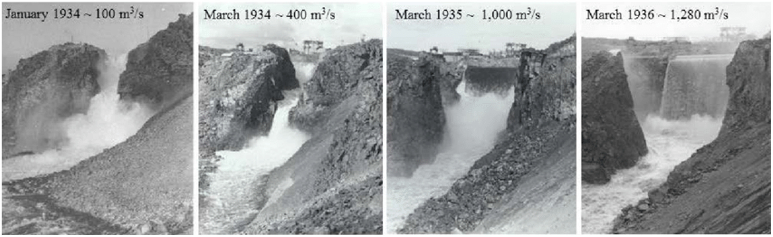
Hydraulic plucking is an important scour mechanism and a critical design consideration for infrastructure interacting with flowing water. Large volumes of competent rock can be eroded quickly to the point at which stability and safe operation of engineered structures is compromised. In particular, scour of unlined rock spillways is known to cause damage that can jeopardize their integrity and continued operation. For example, Ricobayo Dam in Spain (Fig. 1) suffered rapid and extensive scour damage to the spillway at flows well below the design discharge (Annandale 2006). Similarly, the unlined spillway at Spaulding Dam, located in the Sierra Nevada Mountains in Northern California, is eroding actively, with erosion occurring during routine discharges (George and Sitar 2016a). Additionally, the near-disaster that occurred at Oroville Dam in Northern California in February 2017 initiated at flows well below the maximum design flow rate (Wahl et al. 2019), and the rapid expansion and deepening of the ensuing cavity was due largely to erosion of hard rock along preexisting joints. These examples illustrate the potential hazard posed by hydraulic plucking and the limitations in how we currently assess when and how it will occur.

Fig. 1. Progressive scour damage to the unlined rock spillway at Ricobayo Dam in Spain. (Reprinted from Annandale 2006, with permission from McGraw Hill.)

Given these limitations, there is a clear need for scour assessment methods that can incorporate local features into engineering design and scour risk assessments to effectively identify the potential for hydraulic plucking. The erodibility index method (Annandale 1995, 2006) is a prominent empirical scour prediction model that is particularly attractive for use in engineering practice due to its simplicity. However, given the empirical nature of this method, it is not able to differentiate between different failure modes and scour mechanisms, so it does not provide information about what remediation might be most beneficial for engineered structures. Comparatively, physical process models (Bollaert 2002; Liu and Li 2007; Li and Liu 2010; Federspiel et al. 2011; Pan et al. 2014; Li et al. 2016) explicitly represent mechanisms that may lead to scour so that their influence may be investigated. However, the shapes of the blocks generally are simplified (either rectangles or cubes), which may not not be representative of the shapes of rock particles within a fractured rock mass. Additionally, simplifying block shapes to two dimensions enforces plane-strains and effectively treats particles as infinite rods. This introduces limitations in the broader applicability of these methods: three-dimensional (3D) geometry of individual particles, formed by the joints and fractures, dictates the kinematic behavior of fractured rock (Goodman and Kieffer 2000; Sitar et al. 2005; Gardner and Sitar 2019b) and the kinematic admissibility of individual rock particle removal (Goodman and Shi 1985). In their scaled flume experiments, George and Sitar (2016b) showed that the three-dimensional orientation and geometry of particles have a significant impact on the ease with which the particles can be hydraulically plucked and dictates the kinematic response. At present, three-dimensional particle geometry, and how it influences the dominant mode of failure, is not considered directly in scour models.

To capture these three-dimensional effects, it is necessary to explicitly incorporate individual particle geometry in scour analyses such that the kinematics are handled naturally and match site conditions as closely as possible. In addition, the influence of the particle shapes and how they interact with fluid should be included in analyses—initial particle orientations will affect fluid flow and, as the particles move, the flow field will be altered, potentially increasing the rate at which scour occurs. Such analyses require direct simulation of the hydrodynamic forces and dynamic interaction of the fluid–rock system. To this end, the discrete-element method (DEM) (Cundall and Strack 1979; Cundall 1988; Hart et al. 1988) and the lattice Boltzmann method (LBM) (McNamara and Zanetti 1988; Succi et al. 1989) are coupled to model the dynamic fluid–solid interaction that leads progressively to hydraulic plucking. This coupled approach is capable of explicitly incorporating three-dimensional particle shape in scour assessments such that kinematic constraints are captured automatically, without the need for rolling resistance models (Sakaguchi et al. 1993; Zhou et al. 1999; Iwashita and Oda 1998; Jiang et al. 2005) as are required when using spherical DEM. Additionally, by using LBM coupled with DEM, the need for remeshing due to large particle displacements and rotations is avoided, which reduces computational cost and potential numerical error incurred during the remeshing process. Nonspherical DEM and LBM can be coupled through a momentum exchange approach (Ladd 1994; Aidun et al. 1998; Ginzburg et al. 2008a), a volume-fraction approach (Noble and Torczynski 1998; Gardner and Sitar 2019a), or immersed boundaries (Peskin 1977; Feng and Michaelides 2004). Here, the momentum exchange approach was used with linear interpolation, as outlined by Ginzburg et al. (2008a), because it has been shown to provide more-accurate results (Peng and Luo 2008).

An additional aspect of assessing the removability of particles by hydraulic plucking is the influence of turbulent flow because conditions often are highly turbulent in both natural and engineered flows that interact with infrastructure. Several models have been developed to consider the influence of turbulent pressure pulses on the erosion of rock from unlined spillways (Bollaert 2002; Bollaert and Schleiss 2003, 2005; Liu and Li 2007; Pan et al. 2014; Fiorotto et al. 2016); however, these models do not directly consider the dynamic evolution of the pressure pulses due to block displacements, nor do they incorporate three-dimensional effects due to block geometry. To describe this three-dimensional, dynamic effect, a large-eddy simulation (LES) approach was implemented in the LBM. In this approach, flow features that occur at scales below what can be resolved directly by the LBM mesh are described through a turbulent eddy subgrid-scale viscosity. Here, the Smagorinsky (1963) LES model was implemented within the LBM framework to account for energy transfer between the resolved and unresolved scales in the fluid model.

These different elements are linked together such that scour analyses can incorporate irregular, three-dimensional particles and how they interact with turbulent flow. This allows for the influence of site-specific characteristics on hydraulic plucking to be addressed directly in scour assessments. Specifically, solid particles are modeled using convex polyhedral DEM such that the correct kinematic response is captured as dictated by particle and boundary geometry. A two-relaxation time (TRT) (Ginzburg et al. 2008a) collision model with Smagorinsky LES is used in the LBM to model turbulent flow. A D3Q27 velocity discretization is used in the LBM to avoid issues associated with rotational invariance in D3Q15 and D3Q19 discretizations (Silva and Semiao 2014), which is known to cause issues in high-Reynolds-number flows (White and Chong 2011; Kang and Hassan 2013; Suga et al. 2015; Krüger et al. 2017). These methods are all implemented together in a customized version of the open source software waLBerla (Bauer et al. 2021), which is a massively parallel computational fluid dynamics framework with the ability to couple fluid simulations with rigid body–dynamics solvers. The features that were added to this framework as part of the work presented here include convex polyhedral DEM, the LES model in the TRT LBM implementation, and coupling of the polyhedral DEM model with the fluid solver. The polyhedral DEM implementation enables analyses that consider how convex polyhedral shape influences particle–particle interactions, and coupling the polyhedral DEM with the LBM fluid solver enables direct simulation of dynamic fluid–solid interaction that explicitly considers particle shape. The addition of the LES model in the TRT model allows higher-Reynolds-number flows to be simulated such that turbulent flow can be modeled during the scour process. By adding this functionality to waLBerla, the parallel computing capability already available through this framework can be leveraged on high-performance computing (HPC) systems, which ultimately makes this class of simulation possible. This polyhedral DEM-LBM-LES model was used to simulate two high Reynolds number (

R \sim 1 \times 10^{6}

and

\sim 50,000

) flows. The first configuration considered a backward-facing step to illustrate how sliding and toppling failure modes are captured automatically by the modeling approach. The second configuration modeled flume experiments considering tetrahedral particles in turbulent flow (George and Sitar 2016b), in which the failure mode was not as immediately obvious. These simulations show that this numerical approach is capable of accurately predicting the dominant failure modes and reproducing observations from the physical flume experiments. The correct predictions of the failure modes were achieved without any a priori assumptions or restrictions on the likely failure mode. Therefore, the presented modeling approach implemented in HPC has the potential for broad yet geographically specific application in scour assessment studies because local features, such as jointing and fracturing within the rock mass and how they interact with surrounding flow conditions, can be assessed directly.

Model for Fractured Rock

The mechanical behavior of fractured rock is governed by the discontinuities within the rock mass—displacements occur along fractures and joints, and the strength of these discontinuities is significantly lower than that of the surrounding competent rock. Given this inherent discontinuous nature of the rock and the highly localized displacements along discontinuities, continuum-based methods cannot capture the full kinematics of rock mass response. The discrete-element method (Cundall and Strack 1979; Cundall 1988; Hart et al. 1988) explicitly accounts for the discrete, particulate nature of fractured rock and is well suited to describe the kinematic interaction between individual rock blocks. Specifically, polyhedral DEM was used here to consider explicitly the shape of rock blocks in a fractured rock mass. In DEM, the Newton–Euler equations are solved for each individual particle in the system, and the interaction of particles with other particles and boundaries is described through collisions and an associated constitutive model for these collision contacts. Essentially, DEM establishes resulting forces and moments on each particle by considering all collisions of the particles with their neighbors, and then integrates individual particle motion after all forces and moments acting on the particles have been resolved. The following sections provide a brief overview of the DEM, focusing on the methods that were applied in this research.

Contact Detection

The process associated with determining which particles are actually physically in contact accounts for approximately 80% of the total simulation time for DEM analyses (Horner et al. 2001). To minimize the number of computations associated with contact detection, the process generally is divided into two phases: (1) a neighbor search aimed at identifying particle pairs that are physically close enough to potentially be in contact; and (2) contact resolution, which takes the list of potentially contacting particle pairs and scrutinizes them further to establish whether particles are physically touching. The general idea in the neighbor search algorithm is to avoid checking particles that are not close enough to realistically be touching. Here, an order

O (N)

hierarchical hash grid (Schornbaum 2009) is used during the neighbor search.

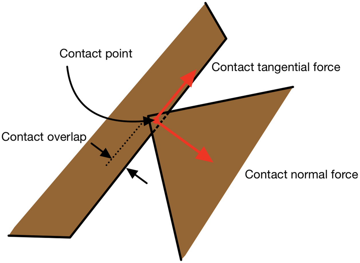
After the neighbor search has established which particles are sufficiently close to potentially be in contact, individual particle pairs from the list of potentially contacting particles are scrutinized further to determine if there is actual contact. To avoid unnecessary computations, the axis-aligned bounding boxes of the particle pair are checked for intersection. If they do not intersect, the particles are not in contact and no further checking is required; if they do intersect, detailed computation is required to assess if the particles are in contact. In this research, contact was checked using the Gilbert–Johnson–Keerthi (GJK) (Gilbert et al. 1988) algorithm, and the contact point, contact overlap, and contact normal were established using the expanding polytope algorithm (EPA) (van den Bergen 2001).

Contact Forces and Moments

The contact geometry calculated during contact resolution (Fig. 2) is input into a contact constitutive model that describes the forces and moments between two particles that are in contact. Given the modular formulation of DEM, it is possible to use a broad array of constitutive models for modeling particle–particle interactions. In the simplest case, contact between two particles is described using linear elastic contact springs that relate the amount of deformation to a contact force, in which the contact springs can be thought of as penalty springs (O’Sullivan 2011). Richer models that can describe hysteresis and time-varying response can be implemented within this framework, and many such models have been developed to consider contact interaction (Walton and Braun 1986; Thornton and Yin 1991; Vu-Quoc and Zhang 1999; Goodman and Kieffer 2000; Barton and Bandis 1987; Plesha 1987; Amadei and Saeb 1990; Jing et al. 1994). Here, a linear spring model in the contact normal direction and Coulomb friction in the tangential direction was implemented, as defined by Hart et al. (1988). The confining stresses acting on the particles are sufficiently low such that contact forces are relatively small and can be assumed to be in the elastic range.

Fig. 2. Contact geometry between two colliding particles. The contact resolution phase establishes the contact point, contact overlap, and contact normal that are used in calculating contact forces and moments.

The forces and moments calculated from the contact model are added to each of the particles participating in the contact. Thus, after all contacts have been considered, the forces and moments acting on an individual particle are the resultant of all contact forces and moments from all the contacts that the particle participates in. The position of individual particles then can be updated independently by integrating translational and rotational motion

{\ddot{x}}_{i} + α {\ddot{x}}_{i} = \frac{F_{i}}{m_{i}} + g_{i} {\dot{ω}}_{i} + α ω_{i} = \frac{M_{i}}{I_{i}}

(1)

where

{\ddot{x}}_{i}

and

{\dot{ω}}_{i}

= translational and rotational acceleration of particle

i

;

F_{i}

and

M_{i}

= total force and moment acting on particle

i

;

α

is a damping constant;

m_{i}

and

I_{i}

= mass and moment of inertia of particle

i

; and

g_{i}

= gravitational acceleration. Particle motion is integrated using a velocity Verlet finite-difference approach (Swope et al. 1982).

Model for Turbulent Flow

Modeling the flow conditions leading up to and during hydraulic plucking requires a numerical model for the fluid that can describe evolving flow conditions as the solid rock particles begin to displace, while also being able to accommodate large rotations and displacements of these solid particles embedded in the fluid mesh. Additionally, hydraulic plucking often occurs during turbulent flow, so it is essential for the fluid solver to be able to model large-Reynolds-number flows. Therefore, the lattice Boltzmann method is used to model the fluid because it is able naturally to accommodate unpredictable and large displacements and rotations of solid particles that move through the fluid mesh. However, to be able to model turbulent flow conditions and resolve flow structures below the scale of the LBM mesh, it is necessary to also implement a large-eddy simulation model within the LBM. The following sections provide an overview of the LBM and how it was applied in this research, and also describe how a LES model was implemented in the LBM to model turbulent flow conditions.

Lattice Boltzmann Method

Unlike other commonly used methods in computational fluid dynamics (CFD) that directly solve the Navier–Stokes equations, the LBM solves a discretized version of the Boltzmann equation that arrives at the same macroscopic solution of fluid flow as that achieved by solving Navier–Stokes equations directly. By discretizing physical space, time, and velocity space, the so-called lattice Boltzmann equation is derived as (McNamara and Zanetti 1988)

f_{i} (x + c_{i} Δ t, t + Δ t) = f_{i} (x, t) + Ω_{i} (x, t)

(2)

where

c_{i}

= discrete set of velocities which limits continuous particle velocity to a carefully selected subset. The lattice Boltzmann equation, like its continuous counterpart, describes the advection and collision of particles. These two steps are performed sequentially at each time step in the LBM, in which the advection step more commonly is referred to as streaming in the LBM literature. The streaming step describes how a population of particles,

f_{i}

, located at

x

moves with velocity

c_{i}

to a neighboring point located at

x + c_{i} Δ t

; the velocity sets are defined such that it takes a single time step for these populations to arrive at neighboring points. The collision step models particle collisions through the collision operator,

Ω_{i}

, by redistributing particles among the particle populations

f_{i}

.

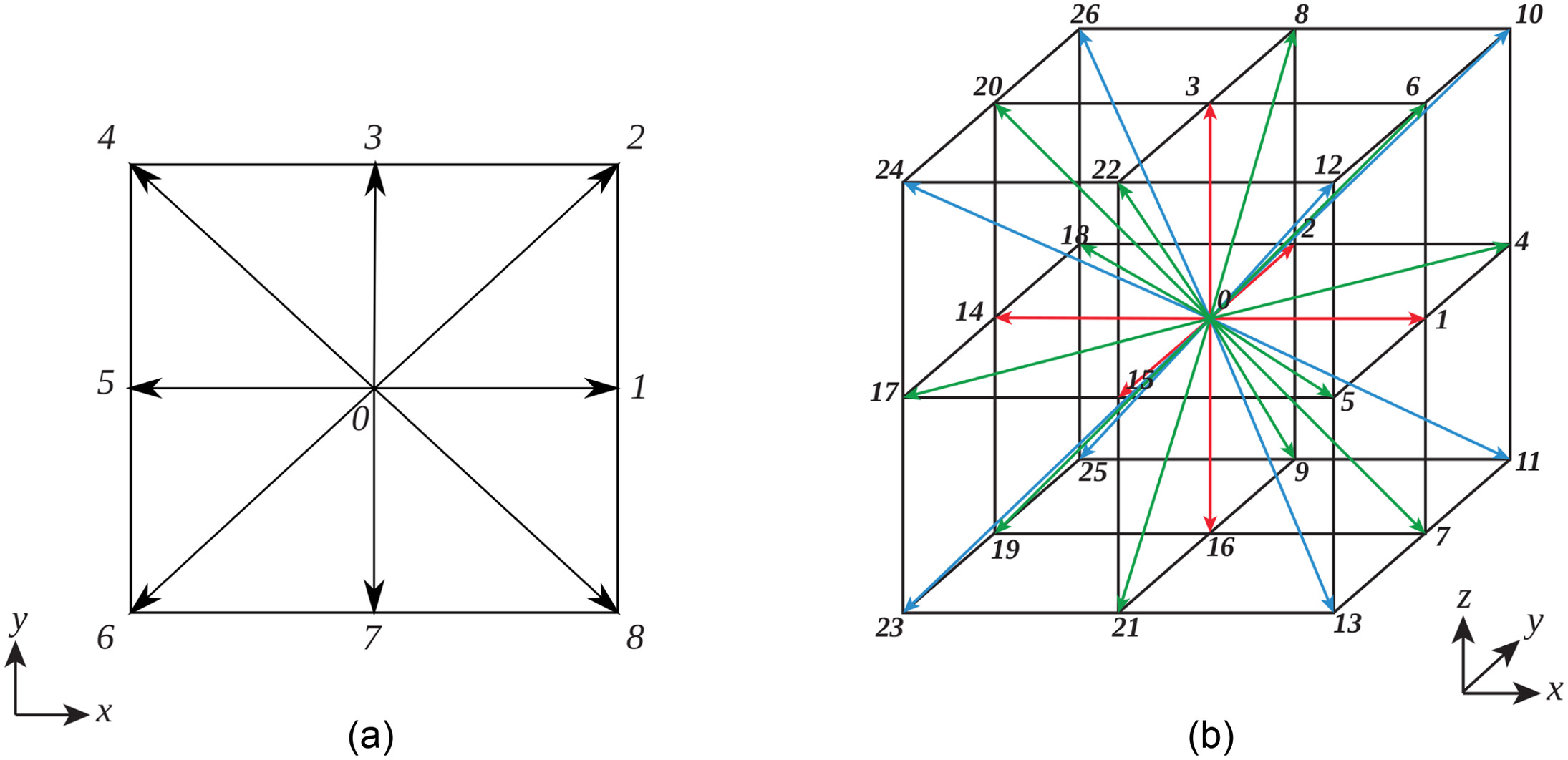
In each fluid cell in the LBM mesh, the discretization of velocity space (Fig. 3) restricts the directions in which populations of particles can stream to a discrete set. How velocity space is discretized impacts both the computational cost and limitations of the LBM in modeling fluid flows. Fewer discrete velocities mean fewer computations and a smaller memory footprint, but this may lead to nonphysical results in specific applications. For example, three-dimensional models with 15 or 19 discrete velocities (D3Q15 or D3Q19) are not rotationally invariant (Silva and Semiao 2014). For large-Reynolds-number flows, this lack of isotropy is known to cause problems: inconsistent results depending on lattice orientations relative to flow (White and Chong 2011), deficient momentum transfer of flow and turbulence (Kang and Hassan 2013), and unsatisfactory accuracy when simulating turbulent flow through pipes and porous media (Suga et al. 2015). Thus, given the potentially highly turbulent flow conditions during hydraulic plucking, a three-dimensional, 27-discrete-velocity set (D3Q27) (Rubinstein and Luo 2008; Suga et al. 2015) was necessary for this research and its larger memory demand is justified.

Fig. 3. Examples of discrete velocity sets in the lattice Boltzmann method: (a) two-dimensional velocity set containing 9 discrete directions in which particles can stream (D2Q9); and (b) three-dimensional velocity set containing 27 discrete directions in which particles can stream (D3Q27). The D3Q27 velocity set was used in this research.

The collision operator,

Ω_{i}

, in Eq. (2) captures the relaxation of particle populations toward equilibrium. This operator is a simplification of the original collision operator in the Boltzmann equation, and is chosen based on the requirements of a particular simulation. The most common and simple collision operator is the Bhatnagar–Gross–Krook (BGK) collision operator (Bhatnagar et al. 1954). However, when using the BGK collision operator, the numerical stability is coupled to the kinematic viscosity, which can become problematic with small viscosities. Additionally, the location of no-slip boundaries is viscosity-dependent when using the BGK collision operator (He et al. 1997), which can lead to nonphysical results—the intrinsic permeability of the porous medium becomes a function of the numerical method and not of the physical properties of the material being modeled. When considering fluid–rock interaction and flow through fractured rock, correctly capturing the physical location of solid boundaries in the fluid simulation is especially important, so the use of the BGK collision operator is not appropriate. To overcome these issues, a two-relaxation time (Ginzburg et al. 2008a) collision model is necessary. The lattice Boltzmann equation for this model then is as follows (Ginzburg 2012):

f_{i}^{*} = f_{i} - λ^{+} Δ t (f_{i}^{+} - f_{i}^{eq +}) - λ^{-} Δ t (f_{i}^{-} - f_{i}^{eq -}) f_{i} (x + c_{i} Δ t, t + Δ t) = f_{i}^{*} (x, t)

(3)

where

λ^{+}

and

λ^{-}

= model parameters; and

f_{i}^{+}

,

f_{i}^{-}

,

f_{i}^{eq +}

, and

f_{i}^{eq -}

= symmetric and antisymmetric parts for populations and equilibrium populations, respectively

f_{i}^{+} = \frac{f_{i} + f_{\bar{i}}}{2}, f_{i}^{-} = \frac{f_{i} - f_{\bar{i}}}{2} f_{i}^{eq +} = \frac{f_{i}^{eq} + f_{\bar{i}}^{eq}}{2}, f_{i}^{eq -} = \frac{f_{i}^{eq} - f_{\bar{i}}^{eq}}{2}

(4)

where

f_{\bar{i}}

and

f_{\bar{i}}^{eq}

= populations with velocity

- c_{i}

. In the TRT collision model, the stability of the simulation is decoupled from the kinematic viscosity such that stability may be achieved regardless of the value of the kinematic viscosity. More importantly, the actual solid boundary (no-slip) location is viscosity-independent in the TRT collision model (Ginzburg and d’Humières 2003; Pan et al. 2006), so that the correct intrinsic permeability is captured. Central to this is the so-called magic number, defined as

Λ = (\frac{1}{λ^{+} Δ t} - \frac{1}{2}) (\frac{1}{λ^{-} Δ t} - \frac{1}{2})

(5)

where

λ^{+}

is related to the kinematic viscosity. The value of the magic number,

Λ

, can be set to optimize for different characteristics in terms of stability and error;

Λ = 3 / 16

results in solid boundaries being located exactly in the middle between solid and fluid nodes (Ginzburg et al. 2008b), and is the value that was used for this research. The value of

λ^{-}

is set to enforce the

3 / 16

magic number based on the kinematic viscosity. The macroscopic Navier–Stokes behavior then is recovered when the kinematic shear viscosity

ν

is related to the

λ^{+}

parameter

ν = c_{s}^{2} (\frac{1}{λ^{+} Δ t} - \frac{1}{2})

(6)

From this mesoscopic description of the fluid, the macroscopic fluid density and momentum are calculated through weighted sums of the particle populations,

f_{i}

, in velocity space

ρ (x, t) = \sum_{i} f_{i} (x, t) ρ u (x, t) = \sum_{i} c_{i} f_{i} (x, t)

(7)

Body Forces

The original LBM does not include body forces; their inclusion manifests as an additional source term in Eq. (2). Several forcing schemes are available (Shan and Chen 1993; He et al. 1998; Guo et al. 2002; Kupershtokh et al. 2009) and have been shown to be equivalent up to second order for the force and third order for velocity (Huang et al. 2011). Thus, for ease of implementation, the forcing scheme proposed by Guo et al. (2002) was used in this research.

Turbulent Flow

The standard LBM is restricted to flows with low to moderate Reynolds numbers and requires special treatment when modeling turbulent flows, as are often encountered during hydraulic plucking. For the range of Reynolds numbers that need to be considered when flow is turbulent, direct numerical simulation of all flow features is not possible because the computational cost to make the LBM mesh sufficiently small is not tractable. To overcome this issue, large-eddy simulation is a popular technique used in computational fluid dynamics to account for this large difference in the scale of flow structures (Pope 2000). In this approach, flow structures larger than the numerical mesh discretization are solved for directly, whereas features at a scale smaller than what the numerical mesh can resolve are accounted for through a subgrid scale model. In the subgrid scale model, the energy transfer between the resolved and unresolved scales is captured through a subgrid-scale turbulent eddy viscosity,

ν_{SGS}

, that is based on the rate-of-strain tensor,

S

. In this research,

ν_{SGS}

was calculated using the Smagorinsky (1963) approach

ν_{SGS} = {(C_{s} Δ)}^{2} | \bar{S} |

(8)

where

Δ

= filtered length scale taken as numerical mesh size;

C_{S}

= Smagorinsky constant, which usually ranges from 0.1 to 0.2 (Scotti et al. 1993); and

\bar{S}

= rate-of-strain tensor. The subgrid-scale eddy viscosity then is incorporated in the LBM through a modified version of Eq. (6)

ν + ν_{SGS} = c_{s}^{2} (\frac{1}{λ^{+} Δ t} - \frac{1}{2})

(9)

The subgrid-scale eddy viscosity is calculated for each cell in the fluid mesh based on the local rate-of-strain tensor. The LBM parameter

λ^{+}

then also is locally modified to incorporate turbulent effects.

Solid–Fluid Coupling

During dynamic fluid–solid interaction, the presence of solid particles in the fluid modifies the flow field in their vicinity, whereas the fluid in turn imparts forces and moments to the solid particles. The hydrodynamic loads on the particles may cause them to move; this induces changes in the flow field, which changes the forces and moments on the solid particles. To capture this evolving interaction between the fractured rock and water, the models for the fractured rock (DEM) and turbulent flow (LBM) need to exchange information continuously throughout the analysis. Here, the momentum exchange method (Ladd 1994; Wen et al. 2014) with a central linear interpolation scheme (Ginzburg et al. 2008a) was used, as described by Rettinger and Rüde (2017). In this method, the exchange of momentum between the solid rock particles and fluid is considered by mapping the particles into the fluid domain such that fluid cells covered by the particles are identified as solid, no-slip boundaries. Because the particle shape is known explicitly, it is possible to calculate the particle velocity at the particle surface and enforce this velocity in the fluid phase. This is achieved by a linear interpolation of the particle populations that enforces the no-slip boundary condition (Ginzburg et al. 2008a).

With the orientation of the solid particles established in the fluid field, the hydrodynamic force acting on a solid particle is calculated following Ladd (1994) as modified by Wen et al. (2014). In this approach, the fluid force contribution for every fluid cell that intersects the solid particle boundary essentially is the difference between momentum toward and momentum away from the solid particle boundary. The total hydrodynamic force,

F

, and torque,

T

, acting on a solid particle then are calculated as the sum of the force contributions of all solid–fluid boundary intersections

F (t) = \sum_{x_{b}} \sum_{j} F_{j} (x_{b}, t)

(10)

T (t) = \sum_{x_{b}} \sum_{j} (x_{b} - x_{c m}) \times F_{j} (x_{b}, t)

(11)

where

x_{c m}

= location of the particle center-of-mass; and

F_{j} (x_{b}, t)

= hydrodynamic force at fluid–solid boundary intersection

j

located at

x_{b}

at time

t

. Thus, the influence of solid particles is considered for each fluid node with which the solids interact, and the resulting hydrodynamic force and torque applied to the solid particles is the aggregated effect from all the fluid nodes with which a particle interacts.

Validation of LES in TRT LBM

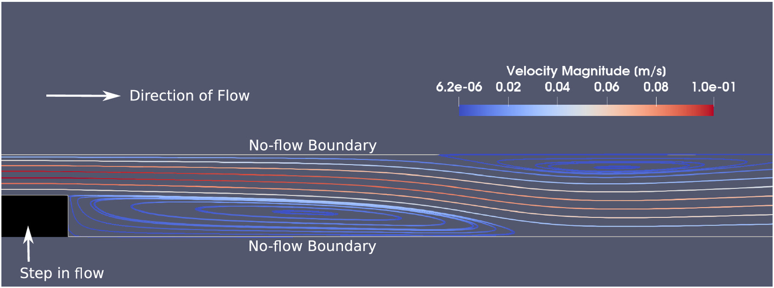
To enable simulations with high levels of turbulence, the LES model developed by Smagorinsky (1963) was used in the LBM. This approach is linked to the TRT collision model within the waLBerla framework such that a subgrid scale viscosity is considered on a cell-by-cell basis throughout the entire fluid domain. Before applying this approach together with the coupled fluid–solid model, it was verified against previous physical and numerical simulations of fluid flow in the vicinity of a backward-facing step to ensure that reasonable results were obtained. For these simulations, an expansion ratio of 2 (i.e., the channel height downstream of the step was twice the height of the channel above the step) was used to compare the results of the TRT with LES with the results from others (Erturk 2008; Rettinger and Nabikhani 2022). Fig. 4 shows a portion of the simulation domain in the vicinity of the backward-facing step. The full simulation domain length was 120 times the step height, with the step located in the left third of the simulation domain. The left boundary was a constant velocity inflow boundary, whereas the right boundary was an outflow boundary. The top and bottom boundaries of the domain in Fig. 4 are no-flow boundaries.

Fig. 4. Configuration for backward-facing step simulations with TRT and LES. Flow moves from left to right in the simulation domain in which the channel height downstream of the step is twice that upstream of the step. Stream tracers shown are for $R = 700$ .

These simulations were run for a range of Reynolds numbers to evaluate the validity of the TRT-LES implementation over a range of velocities. For each of these simulations, the normalized recirculation length was calculated and compared with previous results (Table 1). The normalized recirculation length was taken as the distance from the bottom of the backward step to the reattachment location, normalized by the step height. The results in Table 1 are the recirculation zone calculated using the TRT-LES implementation and the BGK implementation without LES (Rettinger and Nabikhani 2022), and experimental data (Erturk 2008). The results show that the numerical results compared well with both the BGK and experimental results; errors compared with the experimental results were less than 1% in all but one case. The TRT-LES implementation also is shown to be able to model flows at a higher Reynolds numbers than the BGK model with no LES.

Table 1. Normalized recirculation length

Reynolds number	BGK	TRT with LES	Literature	% difference between BGK and literature	% difference between TRT with LES and literature
100	2.880	2.89	2.922	1.44	1.10
400	8.180	8.17	8.237	0.69	0.81
700	11.080	11.11	11.129	0.44	0.17
1,000	13.040	13.07	13.121	0.62	0.39
1,500	—	15.845	15.916	—	0.45
2,000	—	18.195	18.336	—	0.77

Note: Rettinger and Nabikhani (2022); and Erturk (2008).

Influence of Mesh Resolution and LES

In addition to the extensive validation that has been done for the existing code in waLBerla (Rettinger and Rüde 2018; Masilamani et al. 2015; Bogner et al. 2015; Fattahi Evati 2017; Peinado Bravo 2019; Rettinger 2013; Gmeiner 2007), a sensitivity analysis of the DEM-LBM-LES approach to mesh size was conducted. A series of analyses was run at varying mesh sizes both with the LES model and without. In these analyses, a cube was placed in a three-dimensional, uniform flow field in which the left boundary was a constant velocity inflow boundary, the right boundary was an outlet boundary, and the remaining boundaries were periodic. This test case provided an ideal configuration for testing the influence of both the mesh and LES model on the calculated drag because numerical values can be compared with extensive experimental data to verify that the results are reasonable. The drag coefficient,

C_{D}

, can be calculated directly from these simulations using the following equation:

C_{D} = \frac{F_{D}}{\frac{1}{2} ρ u^{2} A_{proj}}

(12)

where

F_{D}

= hydrodynamic drag force exerted on cube;

u

= flow speed;

ρ

= density of fluid; and

A_{proj}

= projected cross-sectional area of the volume-equivalent sphere of the cube. Fig. 5 shows the numerical setup for these simulations, in which the upstream side of the cube is perpendicular to the inflow velocity. Fig. 5(a) shows the overall domain with the numerical mesh for the finest grid spacing. A two-dimensional section is shown in Fig. 5(b) that is zoomed in on the cube to illustrate the mesh size relative to the cube.

Fig. 5. Numerical setup for testing influence of mesh resolution on simulations with and without LES: (a) three-dimensional mesh showing cube in the center of the domain, in which the left boundary is a constant velocity inflow boundary, the right boundary is an outlet, and all remaining boundaries are periodic; and (b) section through domain showing magnified view of mesh in the vicinity of the cube, in which the block side length is 1.0 unit and the mesh discretization is 0.05 units ( $Δ x = 0.05$ ).

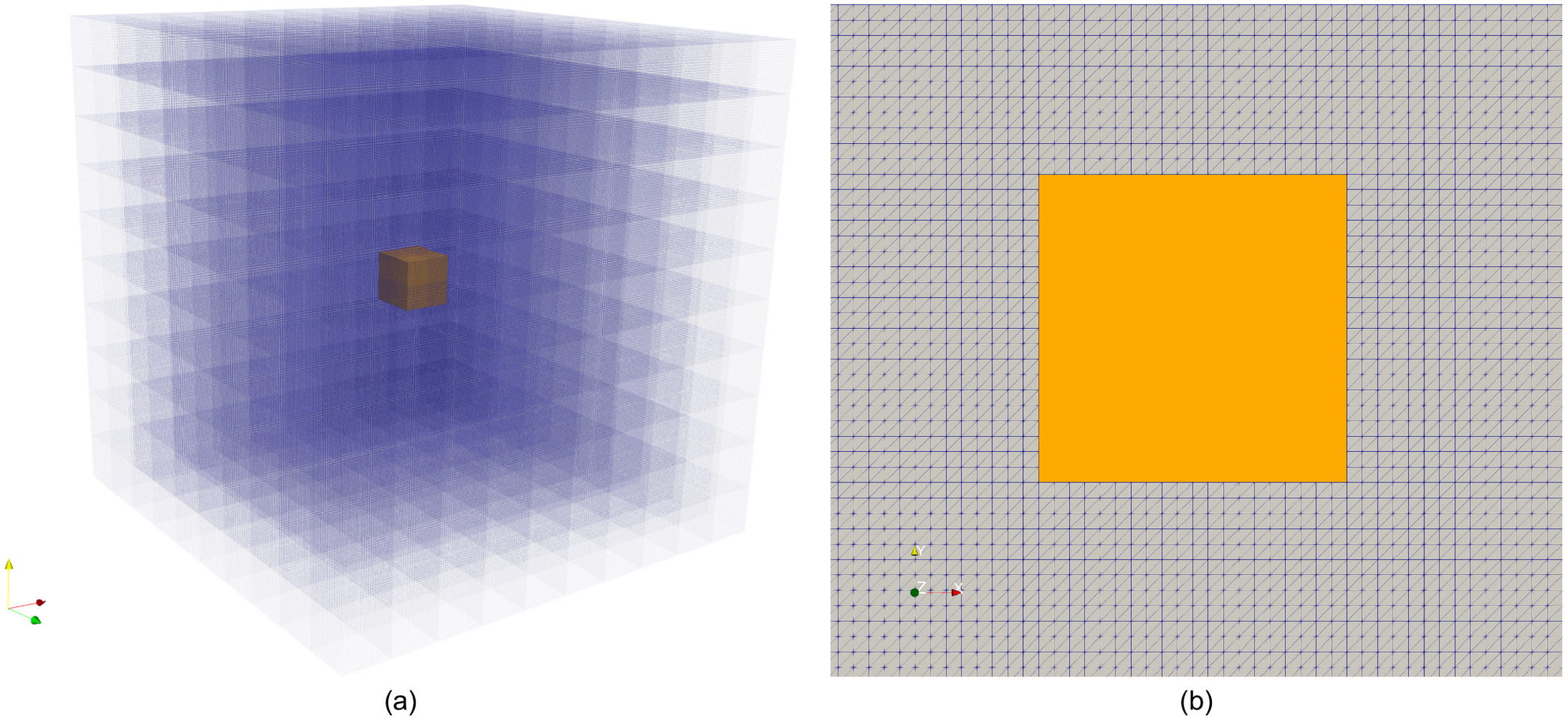
For these simulations, the mesh discretization was set to 0.5, 0.2, 0.1, and 0.05 units; the cube had a side length of 1.0. Because both the drag coefficient and Reynolds numbers are dimensionless, the physical units do not matter as long as they are consistent, and therefore they are not specified here. For all the mesh sizes, the simulation was run with and without the LES model over a range of Reynolds numbers to evaluate the influence of the mesh and LES on the calculated drag coefficient. The results of these simulations are shown in Fig. 6. The numerical results are plotted together with regressions on experimental results (Ganser 1993; Haider and Levenspiel 1989; Hölzer and Sommerfeld 2008) to verify that the values fell within a reasonable range.

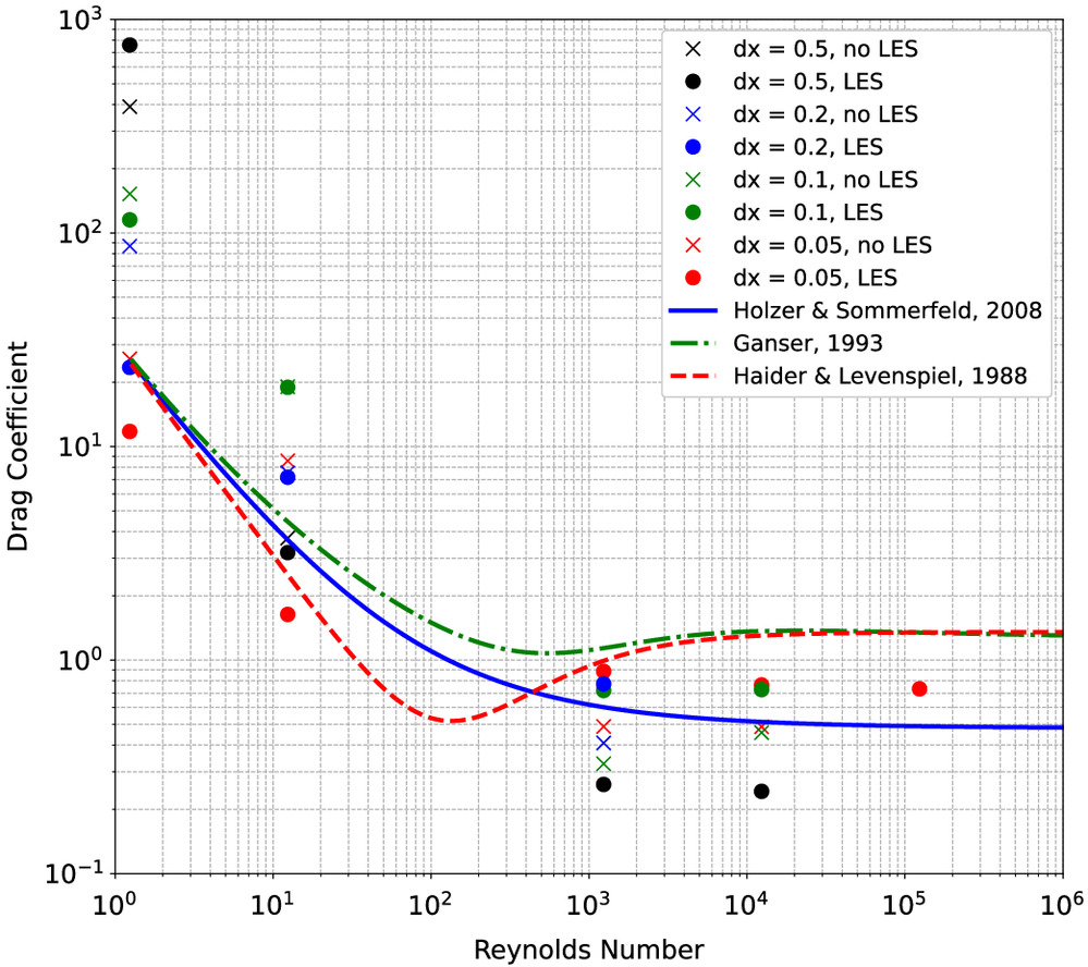
Fig. 6. Numerically calculated drag coefficient, $C_{D}$ , for varying grid resolutions with and without LES compared with regressed experimental data.

In terms of the mesh size, the coarser meshes performed more poorly at lower Reynolds numbers and experienced numerical stability issues at higher Reynolds numbers, especially when no LES model was used. For the cases tested, when the Reynolds numbers were higher than

10^{4}

, the three coarsest meshes failed due to numerical instability in the absence of a LES model. For the finer meshes used, the drag coefficient values were reasonable over the range or Reynolds numbers tested and provided the best estimate of the drag coefficient in general. Stability issues were observed at higher Reynolds numbers even for the finest mesh when a LES model was not used. For higher Reynolds numbers, the finer meshes with LES provided better estimates of the drag coefficient than did simulations that did not use LES, which tended to give lower estimates of the drag coefficient. These simulations show that for typical larger-Reynolds-number simulations, it is necessary to adopt a finer mesh and use a turbulence model, because numerical stability and/or accuracy may suffer otherwise.

Kinematic Analysis of Hydraulic Plucking in Turbulent Flow

The coupled DEM-LBM-LES model was used to analyze two instances of turbulent flow to examine the kinematic response and dynamic evolution of hydraulic plucking. The first scenario considered hydraulic plucking at a backward-facing step. In this case, the only kinematically admissible failure modes based on the geometry of the particle and step were either sliding or toppling. This provided an ideal scenario to evaluate the ability of the modeling framework to correctly predict the failure mode from a simple set of admissible failure modes. The second scenario modeled physical flume experiments conducted by George and Sitar (2016b) of three-dimensional particles hydraulically plucked in turbulent flow. For this scenario, the mode of failure was more complicated and changed based on three-dimensional block orientations, so this set of simulations showcased how the numerical approach is able to capture correctly more-complicated plucking modes in which the likely mode of failure is not as immediately obvious.

In terms of parameter settings for these simulations, the numerical parameters that required calibration were minimal. For the fluid phase, the TRT collision model in the LBM has two input parameters. The first parameter,

λ^{+}

, sets the viscosity of the fluid, which was set in this case to match the kinematic viscosity of water at 20°C. The second parameter,

λ^{-}

, was set to ensure that the solid boundaries were enforced exactly midway between fluid nodes, as discussed in the section “Solid–Fluid Coupling.” For the solid phase, the DEM model requires the friction angle for the solid material, the normal and tangential contact springs, and damping constant. The friction angle values used in each of the simulations are discussed in the appropriate sections subsequently. The normal and tangential contact springs were set to the minimum values that ensured minimal overlap between contacting particles, and essentially functioned as penalty springs (O’Sullivan 2011). Lastly, the damping constant,

α

, as discussed in the section “Model for Fractured Rock,” was set to 0.02.

Erosion in the Vicinity of a Backward-Facing Step

When rock jointing and fracturing is almost parallel and vertical to the slope surface, the dominant modes of hydraulic plucking are toppling (Lamb and Dietrich 2009) and sliding (Dubinski and Wohl 2013). This configuration is illustrated in Fig. 7, which shows a backward-facing step with a single block located on the downstream side of the step. Here, the kinematic constraints due solely to the geometry of the block and backward-facing step are such that only toppling or sliding are the possible modes of failure. Which of these occurs depends on the geometry of the individual block and boundaries and on the flow conditions. The DEM-LBM-LES simulation approach was used to model this configuration to determine whether the modeling approach is able to correctly distinguish the correct failure mode without constraining the potential movement of the erodible blocks. The modifications added to waLBerla make it possible to consider different block shapes within the turbulent flow, and the dynamics of how blocks erode in turbulent flow. Here, two configurations were considered that had two different dominant failure modes: one failing by toppling, and the other failing by sliding.

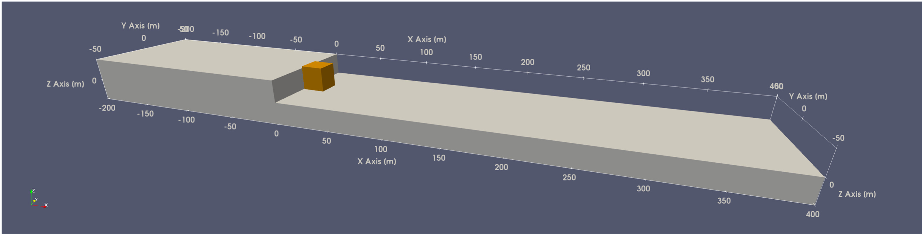
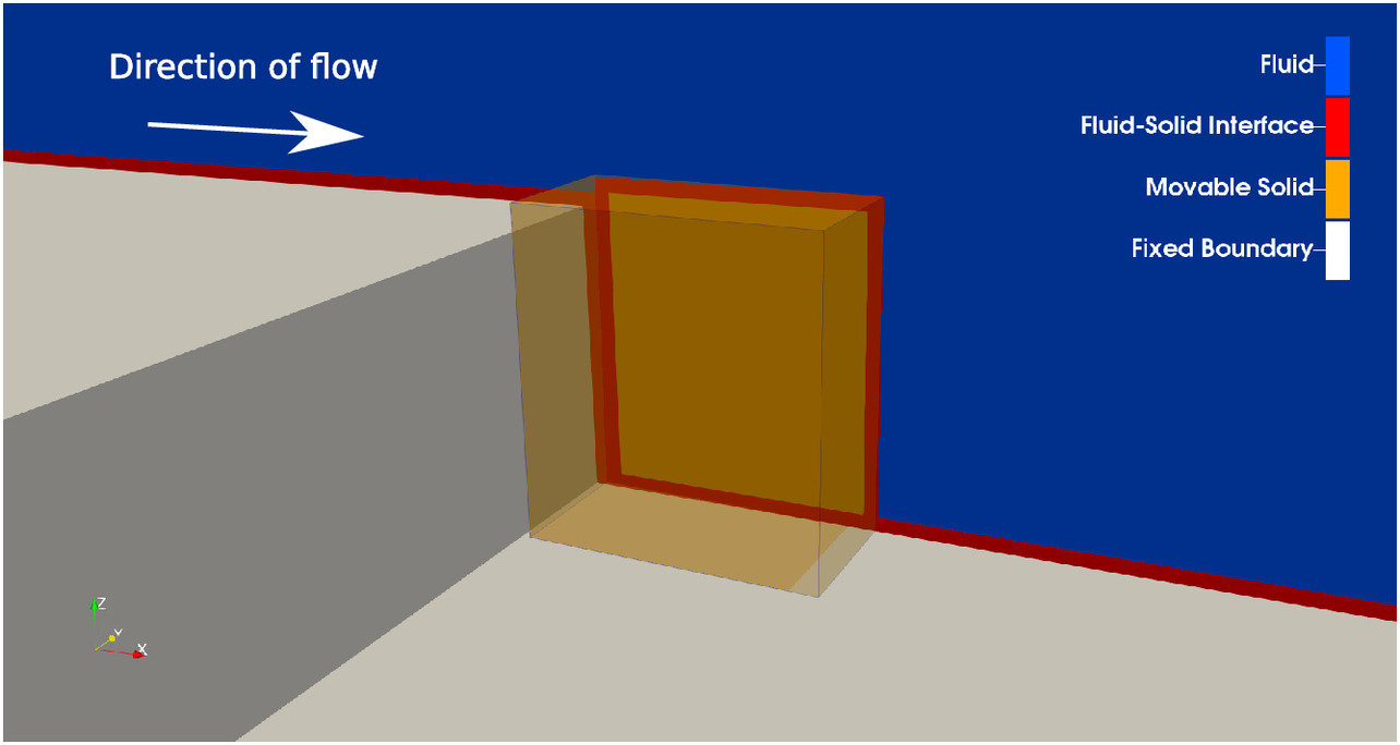
Fig. 7. Simulation domain showing block located at backward step. Inflow boundary is on the left, and outflow boundary is on the right.

The numerical setup (Fig. 7) for these simulations was as follows. The left boundary enforced a steady-state open channel velocity profile based on the slope angle (12° in this case); the right boundary was an outflow boundary; the top boundary was modeled as a free-slip boundary; and the flow-parallel vertical boundaries (front and back) were treated as periodic boundaries. The solid particles that formed the backward-facing step were mapped into the fluid domain as fixed boundaries, whereas the erodible particles were mapped into the fluid domain as movable solid particles (Fig. 8). This mapping also shows fluid–solid interface cells where the exact particle boundary is mapped based on the coupling algorithm described previously. The numerical grid size was 0.05 m, which equates to approximately 20 fluid cells/side of the movable solid block. An important feature in this simulation framework was the ability to set the fracture aperture, which defines the effective space available for fluid to flow between the individual solid particles. In polyhedral DEM. the faces of the particles are perfectly planar and thus do not allow for fluid to flow through fractures when particles are perfectly flush; however, in real rock masses, surface asperities and joint undulations allow for some amount of fluid to flow through the fractures. To capture this effect, the initial fracture aperture can be set to allow fluid flow along these planar contacts. When setting the fracture aperture, the block sides are shifted toward the center of mass of the particle when mapped into the fluid domain. This creates space for the fluid to move between particles so that fracture flow can be incorporated in simulations. The true locations of the block sides still are used in solid–solid contact calculations, and the fracture aperture changes during the simulations as blocks move.

Fig. 8. Cross section perpendicular to flow direction showing how block and fixed boundaries are mapped into fluid domain for backward-facing step.

In the first configuration [Fig. 9(a)], the block experienced sliding downstream due to fluid shear across the top and along the sides of the block as well as transient pressures in the gap between the block and the fixed boundary. The friction angle between the block and sliding plane was 16°, so in the absence of hydrodynamic loads the block would be stable due to frictional resistance between the bottom of the block and the fixed boundary. However, due to hydrodynamic loading, the block experienced a pure translational, sliding failure as it was plucked. In the second configuration [Fig. 9(b)], the block was identical except that the width of the block in the downstream direction was 25% the width of the block in the first configuration. This block underwent toppling failure due to fluid shear from water flowing over and around the block, which induced sufficient moment to rotate the block around the downstream edge. In both simulations, the three-dimensional vortex structure in the vicinity of the blocks is shown through contours of the Q-criterion (Hunt et al. 1988), which is defined as the second invariant of the velocity gradient tensor. Positive values of the Q-criterion indicate vorticity-dominance in the flow field, which is evident in the vicinity of the blocks. The Reynolds number in these simulations was on the order of

\sim 1 \times 10^{6}

, and thus in the turbulent regime.

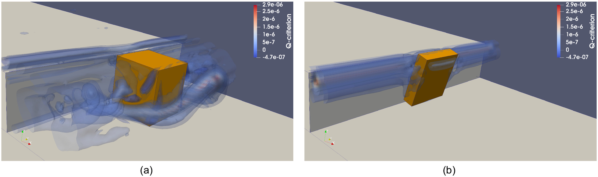
Fig. 9. Different failure modes during hydraulic plucking at backward-facing step: (a) sliding failure mode; and (b) toppling failure mode. Which failure mode is dominant depends on the rock particle geometry. Boundary conditions are identical for both simulations; the only difference is the width of the particle in the downstream direction.

In both simulations, the mode of failure was determined naturally from the analyses without any a priori restrictions on how the blocks were allowed to move—the correct failure mode was captured by the method based on the geometry of the rock blocks and solid boundaries, flow conditions, and the mechanical properties of the solid–solid interaction. How different features contribute to plucking in this setting is an active research topic, and Hurst et al. (2021) showed how, in two dimensions, the mode of failure depends on characteristics of both the solid block and flow conditions. The numerical approach presented here has the potential to build upon this work by directly considering three-dimensional effects and how block motion influences fluid loads acting on the particles both during and post plucking.

Comparison with Flume Experiments of Three-Dimensional Block Erodibility

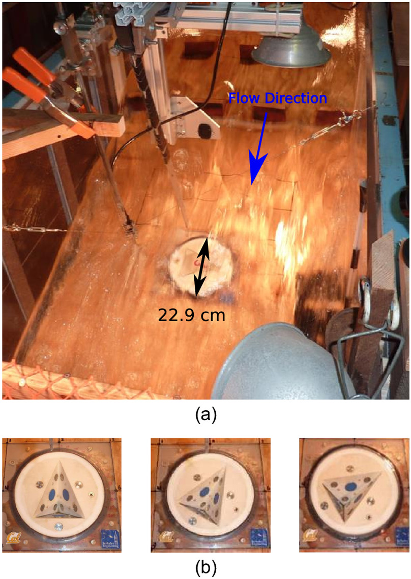
When considering three-dimensional geometry of more-complex-shaped rock blocks and how they interact with water during hydraulic plucking, the dominant mode of failure is not as intuitively identified as was the case with the backward-facing step. This is illustrated in the physical flume experiments conducted by George and Sitar (2016a), in which they investigated the influence of particle geometry and orientation relative to flow on the erodibility of individual particles. In the experimental setup (Fig. 10), 3D-printed tetrahedral blocks were placed in a mold that could be rotated 180° so that the orientation of the blocks relative to the flow direction could be varied. The overall channel grade was 22% at the block location, the friction angle between the block and mold was determined to be approximately 16°, and Reynolds numbers ranged from

\sim 2.0 \times 10^{4}

to

3.0 \times 10^{5}

(George and Sitar 2016a).

Fig. 10. Experimental setup for flume experiments performed by George and Sitar: (a) flume configuration looking upstream; and (b) mold for tetrahedral blocks shown in different orientations. (Modified from George and Sitar 2016a.)

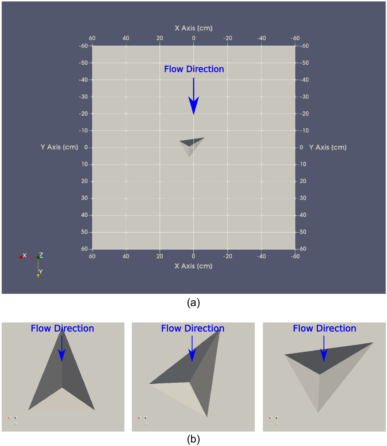
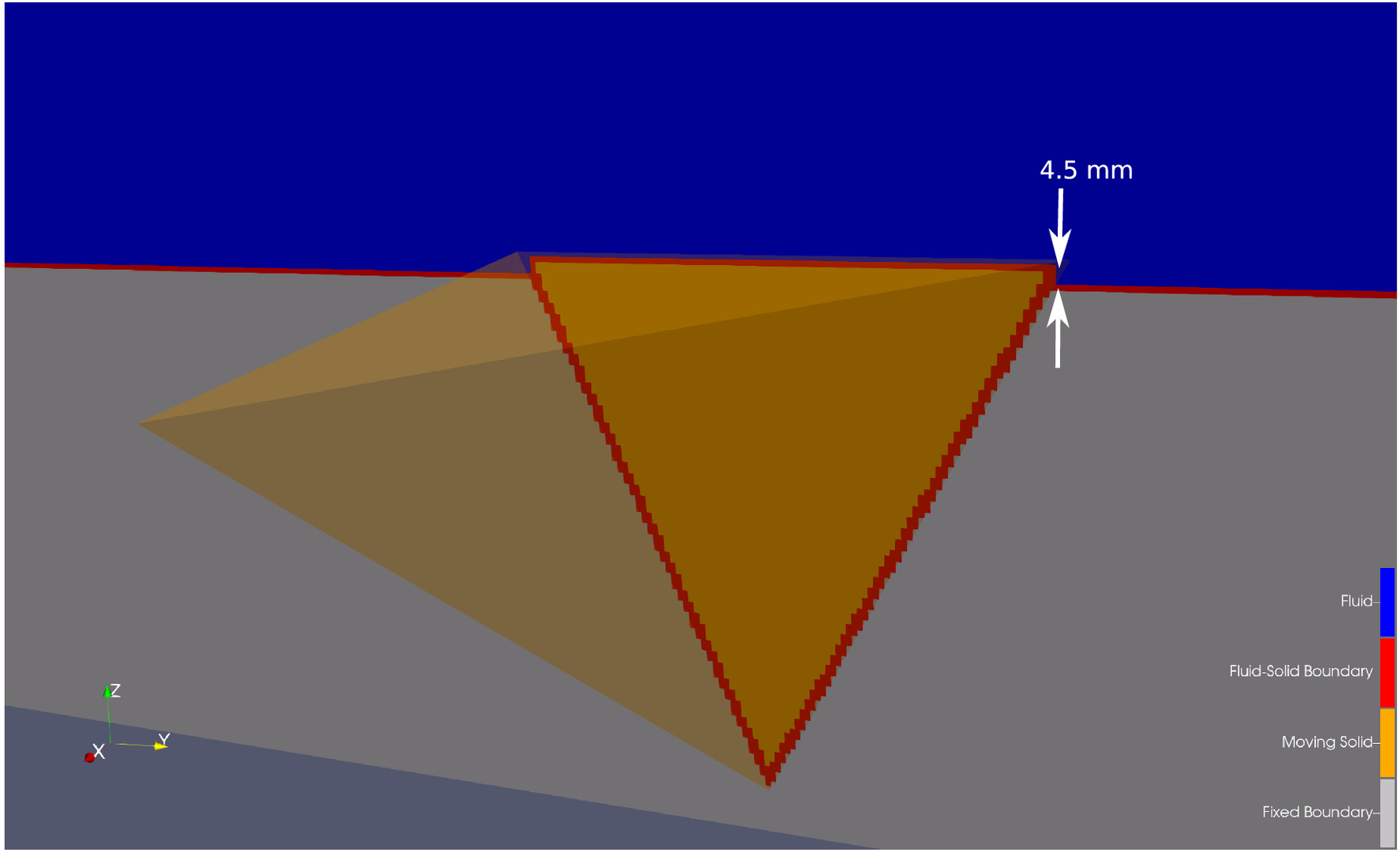
Numerical simulations of these flume experiments were conducted to establish whether the modeling approach is capable of reproducing observations from the physical flume experiments and predicting the correct failure mode. Fig. 11(a) shows the plan view of the numerical model configuration, and Fig. 11(b) shows the different block orientations that were modeled numerically. For these simulations, a mesh size of 1 mm was used, which yielded approximately 100 fluid cells/side of the moveable tetrahedral block. The block protrusion was 4.5 mm above the flume floor (Fig. 12). In the physical flume experiments there was an opening between the block and mold of approximately 2 mm. To simulate this opening in the numerical model, the previously discussed cafterafterpt of fracture aperture was used to allow fluid to flow through the openings between the solid particle and the flume mold. A fracture aperture of 2 mm was used in the numerical simulations to match the configuration in the physical experiments. The mapping of the tetrahedral particle into the fluid domain is shown in Fig. 12. Although Fig. 12 shows a staircase for the mapping, the actual particle surface location was considered in the fluid computations using the solid–fluid coupling scheme previously discussed. Thus, the fluid–solid boundary cells identified in which cells the solid surface fell, then the fluid–solid coupling computations established the location based on the interpolated no-slip boundary. The vertical boundaries of the simulation domain were treated as periodic so that the flow started from rest and then accelerated due to gravity until achieving a steady state. The top boundary was simulated using a free-slip boundary condition.

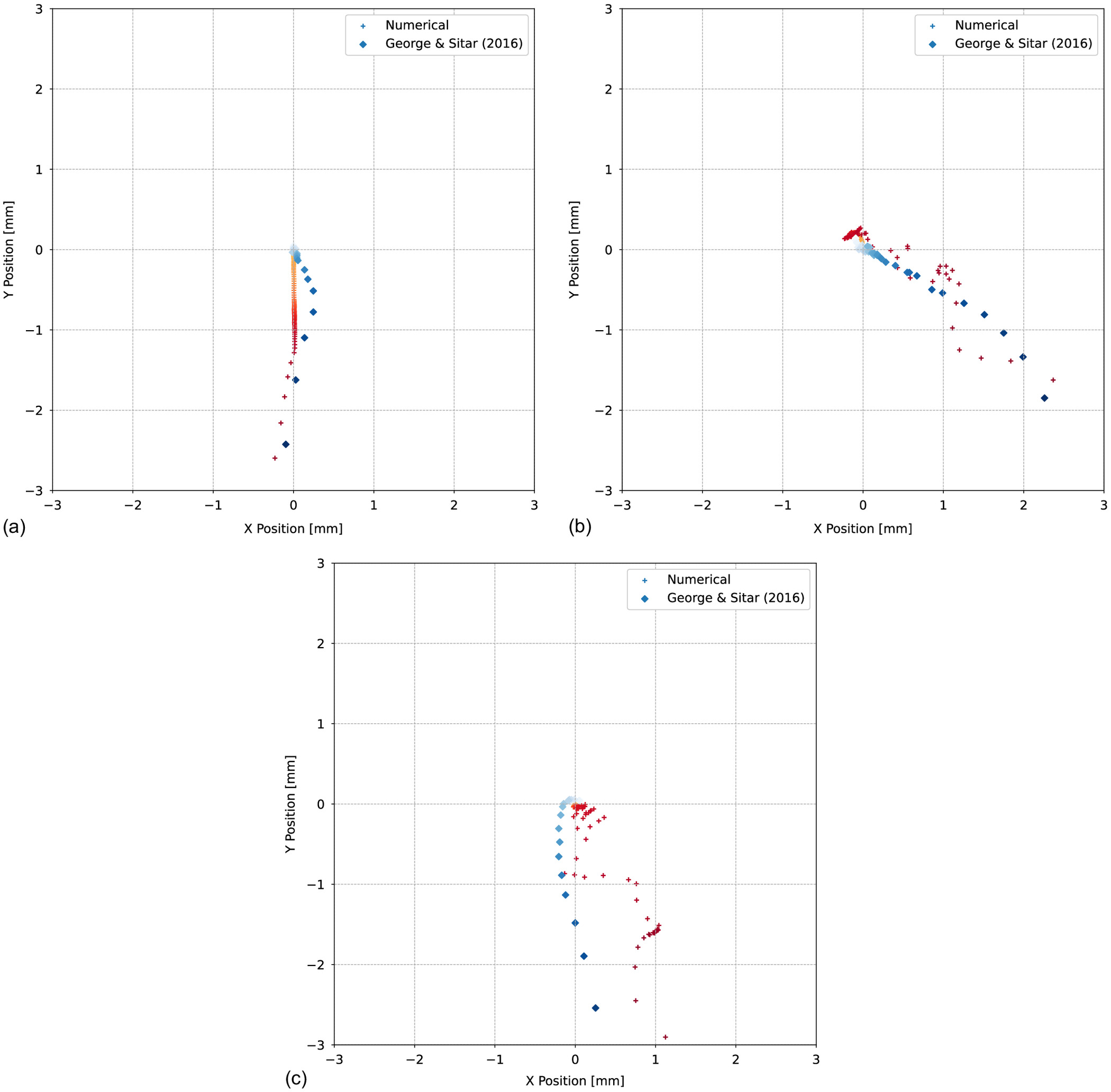
Fig. 11. Numerical model configuration for flume experiment simulations: (a) plan view of experimental configuration, showing the mold rotated to 60°, but the same boundary scale was maintained in all simulations; and (b) mold orientations 0°, 30°, and 60°, from left to right.

Fig. 12. Vertical slice through flume mold and block to illustrate how particle is mapped into fluid domain and how fracture aperture creates joint between block and mold to model the joint that was present in the physical flume experiments. Block protrusion above the flume boundary also is indicated.

The displacement results from the numerical simulations were compared with those from the physical experiments for each of the block responses observed by George and Sitar (2016a) (Fig. 13). Fig. 13 shows good agreement between the numerical simulations and the physical flume experiments in terms of the trends of the displacements. As in the physical experiments performed by George and Sitar, three different block responses were observed. Response 1 [Fig. 13(a)] involved relatively low kinematic resistance to movement downstream, and gradual displacement occurred in a consistent direction. Response 2 [Fig. 13(b)] involved blocks that had a higher kinematic resistance to erosion that also experienced gradual displacement, but block displacement was considerably more variable. In Response 3 [Fig. 13(c)], block response was more dynamic and erratic, and block movement typically occurred due to hydraulic impulses associated with turbulence. As was the case with the backward-facing step, these modes of failure were captured correctly by the numerical implementation without any prior assumptions or restrictions on the likely mode of failure—this is a particularly useful feature of this numerical approach because it is able to capture naturally the dominant kinematic response, which can guide and inform engineering design and scour remediation.

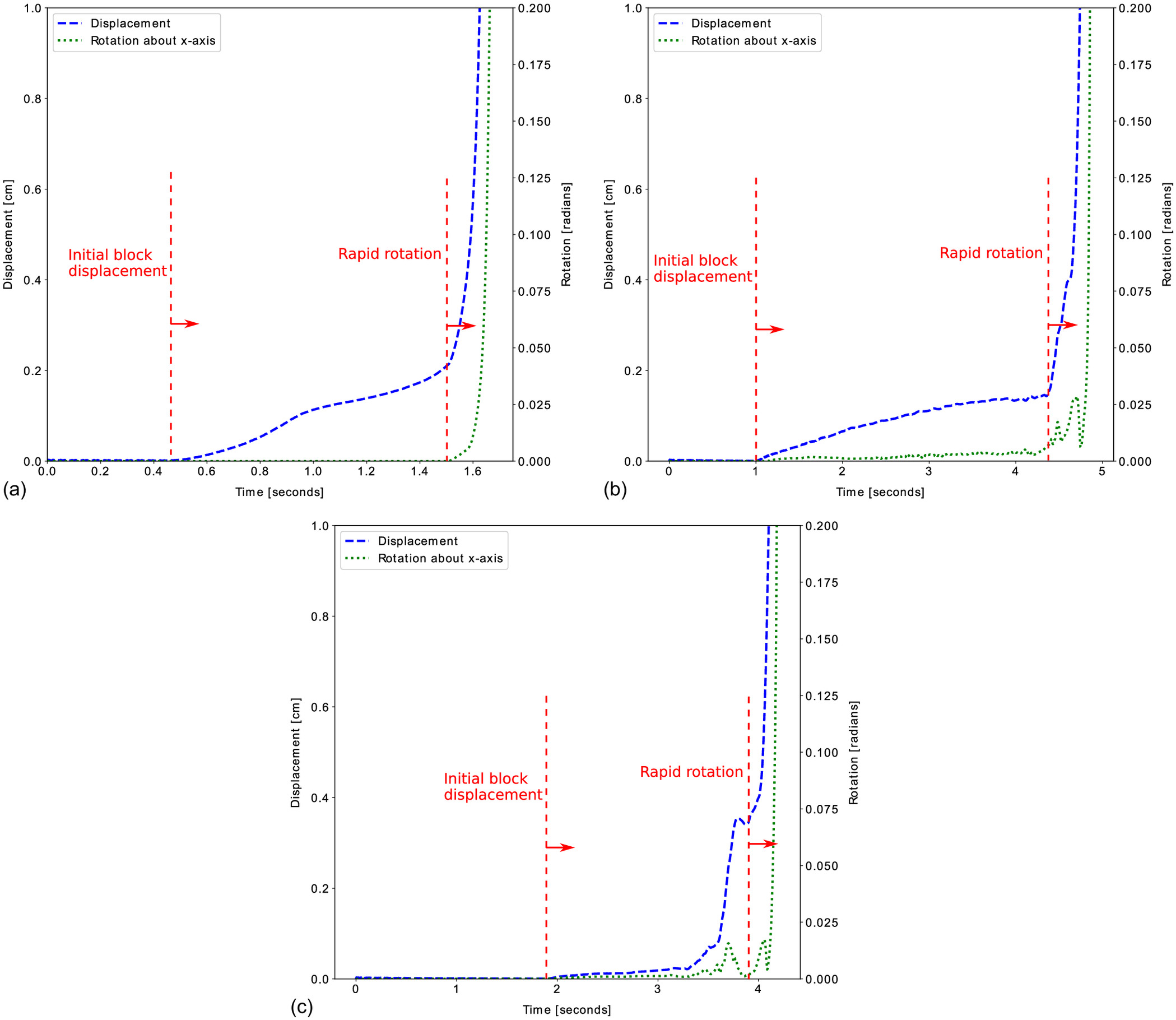
Fig. 13. Numerical block response and response observed by George and Sitar (2016a): (a) block response 1 for 60° orientation; (b) block response 2 for 0° orientation; and (c) block response 3 for 30° orientation. For both physical flume experiments and numerical results, the block center of mass is initially at position (0, 0) and subsequent locations represent block location with increasing time.

The transient nature and differences in the block response are more clearly evident in plots of total block displacement over time (Fig. 14). Here, the time series of numerical block displacements for the three different block responses are shown. The block displacements increased gradually in the case of Block responses 1 and 2, whereas they were more erratic in the case of Block response 3. The initiation of block displacement and rapid rotation are indicated in Fig. 14, and it is clear that in all cases the initiation of displacement preceded the initiation of significant rotation. For Responses 1 and 2, the rapid increase in displacement tended to coincide with the rapid increase in rotation. This indicates that the blocks initially experienced gradual displacement, and only afterafter the blocks sufficiently translated upward into flow did they begin to rotate out of the mold during plucking. In the case of Response 3, the block displacements initiated suddenly and erratically, and initiation of significant rotation was not coincident with initiation of rapid block displacement; this impulse-driven response is consistent with observations by George and Sitar (2016a). The timing at which impulses occurred for Response 3 in the numerical simulations did not coincide with that in the physical experiments for the early phases of displacement. In the physical experiments, submillimeter-scale displacements during hydraulic impulses often were separated by tens to hundreds of seconds, and the numerical approach did not appear to capture this detail. This likely is related to the inability of the numerical implementation to capture every detail of the interaction between the turbulent fluid and solid particles which is exacerbated in the most kinematically resistant cases. However, the initiation of rapid displacement in Block responses 1 and 2 was better captured by the numerical simulations and is consistent with physical observations.

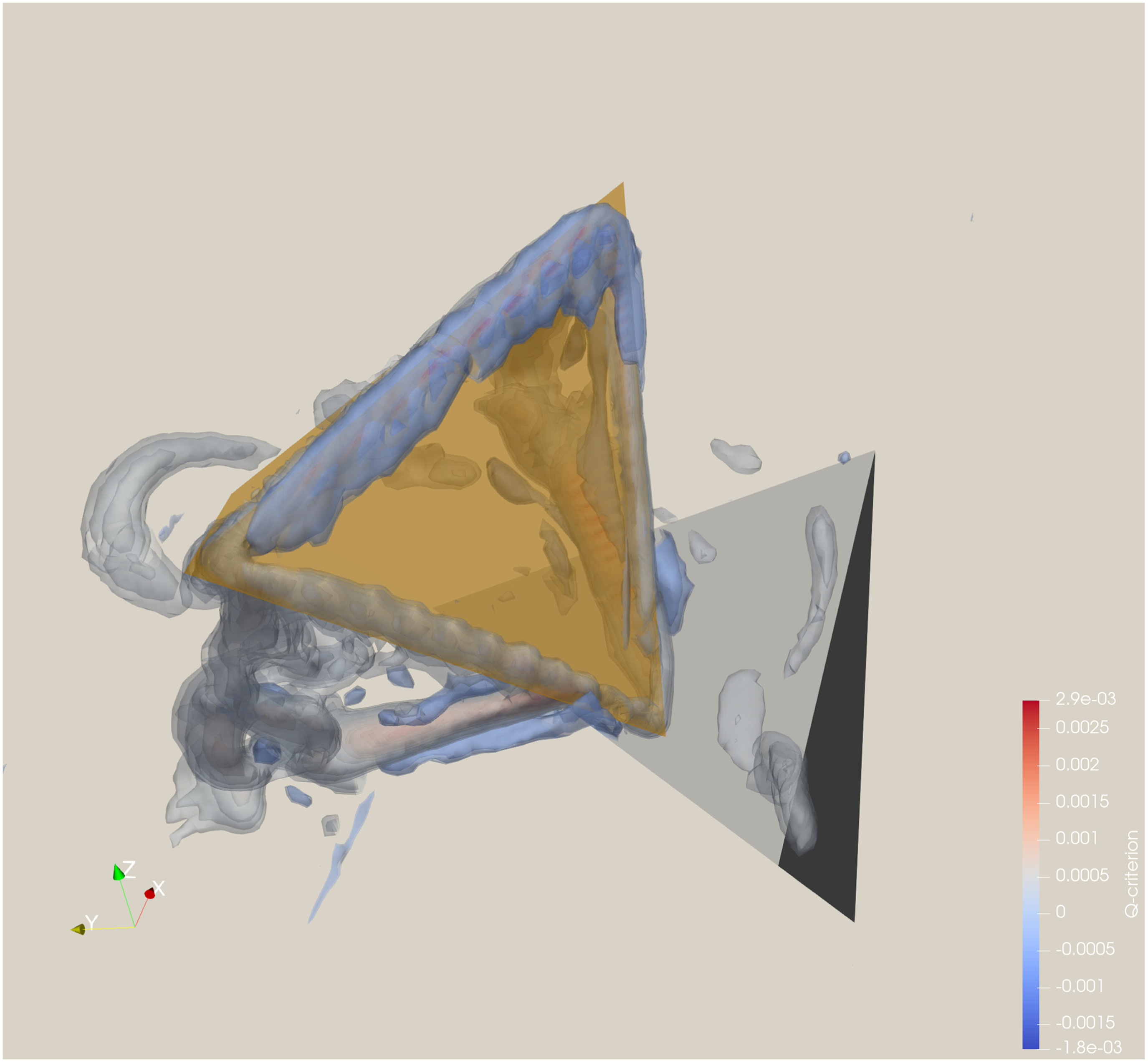
Fig. 14. Block displacement and rotation about $x$ -axis over time: (a) Response 1 transient displacement for 60° mold rotation; (b) Response 2 transient displacement for 0° mold rotation; and (c) Response 3 transient displacement for 30° mold rotation. Block displacements for Responses 1 and 2 initially are gradual and increase rapidly afterafter blocks have translated sufficiently upward into flow. Rotations initiate only afterafter blocks have displaced sufficiently to be plucked by flow. For block response 3, the block displacements are more erratic.

The initiation of displacement prior to rotation was observed both in the physical and numerical simulations. Fig. 15 shows snapshots from both the physical and numerical experiments that show initial sliding followed by simultaneous rotation and sliding as the block is plucked and transported downstream, illustrating how the numerical simulations replicate the observed failure in the flume. Fig. 15 also shows the vortex structure in the vicinity of the block through contours of the Q-criterion. The predominantly positive values clearly illustrate the vorticity dominance in the flow-field around the block, in which vortex shedding over the top surface of the block is shown through the Q-criterion contours. The background in Fig. 15 is shaded based on pressure to show the pressure field surrounding the block during the plucking process. The migration of pressure pulses through the fractures are shown by the alternating lower and higher pressure values; pressure on the upstream side of the block increased steadily as the block moved farther up and into flow. Animations that show transient block motion for the three mold orientations modeled are available in the Supplemental Materials. These animations show the movement of the blocks in plan view as they are plucked. Additionally, one animation shows the transient vortex structure for the 60° mold orientation during plucking.

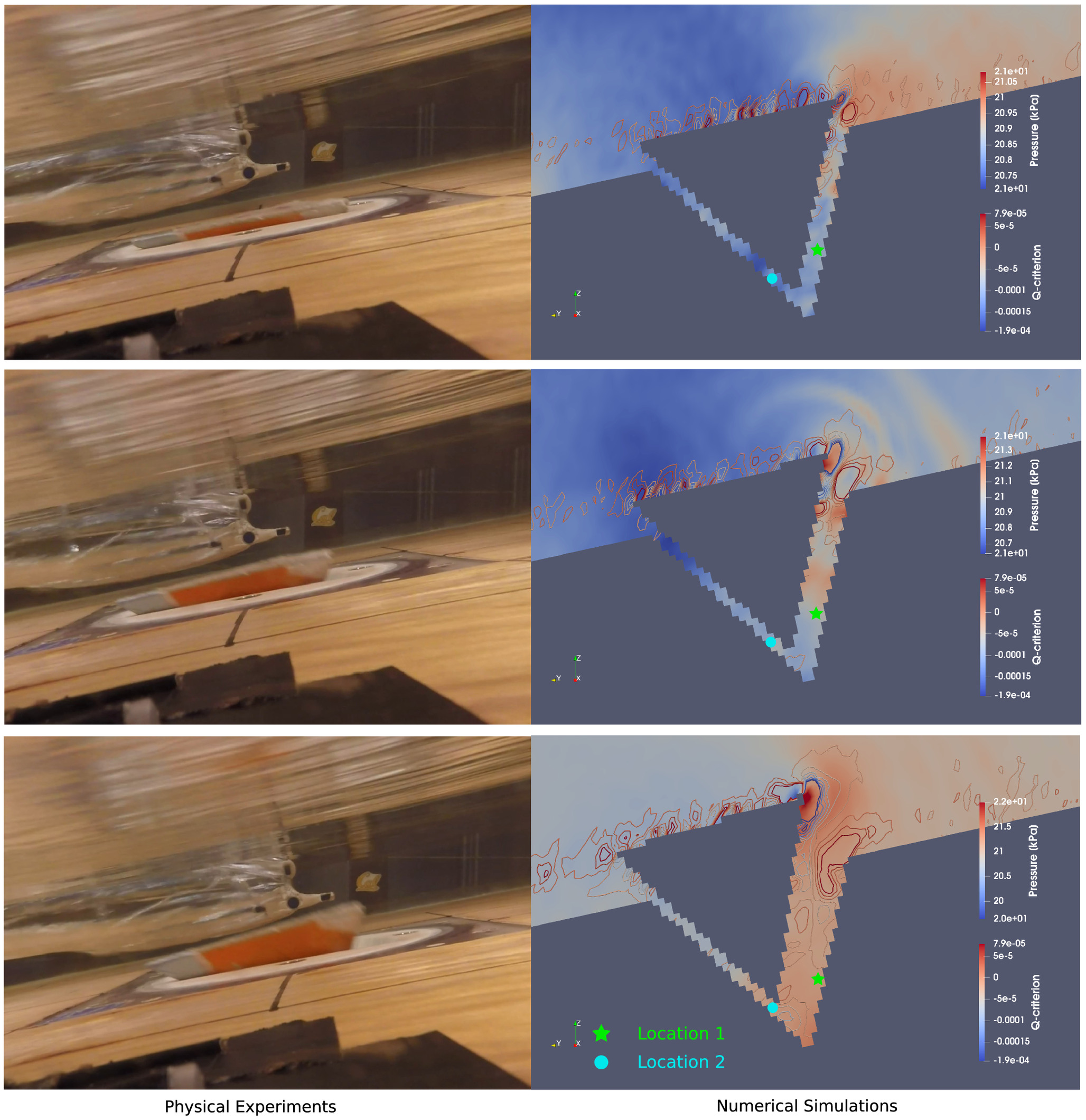
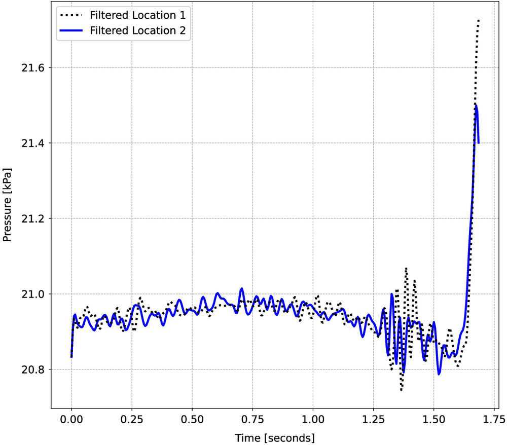
Fig. 15. Comparison of physical and numerical flume experiments. Streamwise section through 3D numerical simulation (shown on the Numerical Simulations) shows how particle initially experiences only displacement and then starts to rotate as it protrudes into flow. This matches what was observed in the physical flume experiments (shown on the Physical Experiments). Contours shown on numerical results are of Q-criterion and background based on pressure. (Physical flume experiment photos courtesy of M. George.)

For the 60° mold orientation, the pressures within the joint between the block and mold were sampled in the numerical simulations at the two locations shown in Fig. 15. Samples were taken at a frequency of 200 Hz and the sampled pressures then were filtered using a Butterworth low-pass filter with a cutoff frequency of 35 Hz. The filtered pressures for the two sample locations are shown in Fig. 16. The pressures are out of phase at the two measurement locations, indicating pressure pulses traveling through the joint between the block and mold. The pressures initially gradually increased, causing the block to begin displacing. After approximately 0.8 s, the pressures decreased slightly, with a subsequent decrease in the rate of block displacement. The magnitude of the pressure pulses increased as the flow became more turbulent due to the evolving block displacement. The variation of pressure within the joint also is shown in Fig. 15. The initiation of progressive block motion appears to be linked to these pressure pulses and increasing pressure within the joint, in which the block slowly was hydraulically jacked up into flow. Due to these pressure-induced movements, the block then sufficiently protruded into flow and was removed completely (Fig. 17). This response is consistent with observations from previous experimental and numerical studies (Bollaert 2002; Liu and Li 2007; Federspiel et al. 2011; Li et al. 2016; George and Sitar 2016a). In addition, the lower pressure above and immediately downstream of the block likely contributes to the initiation of block motion because it creater suction on the block (Fig. 15). The amount of block protrusion above the flume surface has a significant impact on the extent of this low-pressure zone; however, further testing is required to determine whether the hydraulic forces and torque due to the protrusion are the controlling factors or if the low-pressure zone it causes drives block erosion. Furthermore, the shape and orientation of the block dictates the admissible kinematic modes in this complex interaction between the fractured rock and fluid. Sensitivity analyses that explore this interaction and relative contribution of different parameters and configurations can provide insight into which factors have the greatest contribution to the overall variability of the observed response. However, this type of analysis requires a large number of numerical samples to obtain meaningful results and, given the computational demand of this numerical approach, necessitates the extensive use of high-performance computing. Current research efforts are focused on this aspect of the plucking process.

Fig. 16. Filtered pressures at Locations 1 and 2, as shown in Fig. 15, for 60° mold orientation. Pressures are out of phase at two measurement locations, indicating pressure pulses traveling through the joint between the block and mold.

Fig. 17. Tetrahedral block being transported downstream after hydraulic plucking. Block is slightly translucent in image to show three-dimensional turbulent vortex structure surrounding block and mold based on contours of the Q-criterion.

Conclusion

Scour by hydraulic plucking is a complex problem that requires various numerical techniques to be coupled in order to consider the interaction between irregular, three-dimensional rock particles and turbulent flow. Here, a numerical framework to simulate this problem given the presence of large, nonregular displacements and rotations was presented that couples three-dimensional, polyhedral DEM with the two-relaxation time LBM to ensure that solid boundary locations within the fractured rock mass are not viscosity-dependent. A LES model was implemented in the TRT LBM to enable simulation of highly turbulent flows associated with hydraulic plucking. This functionality was implemented in a customized version of the massively parallel, open-source framework waLBerla to leverage high-performance computing resources for these computationally intensive simulations. By using the waLBerla framework and the presented numerical approach, three-dimensional rock particle shape can be incorporated explicitly in both the fluid and solid models. Together, this allows for site-specific characteristics to be incorporated directly in scour assessments.

This framework was applied to two different scenarios of hydraulic plucking that involved progressively more complex modes of failure, illustrating the capability of this approach in correctly capturing the kinematic response based on the fractured rock mass geometry, flow configuration, and mechanical properties. The dominant kinematic modes and transient displacements were captured correctly in numerical simulations of physical flume experiments without restricting the potential modes of failure—the observed response from the numerical simulations was captured naturally based on the input geometry and mechanical properties, and how these interplay with turbulent flow. The capability of this approach to capture the kinematic response without the need to constrain the likely mode of failure makes it especially useful in scour analyses because it offers insight into how local features contribute to scour. This insight into how localized features influence the scour process is particularly beneficial for remediation work and risk analyses because it can help identify the governing mode of failure and guide the choice of the most effective repair or remediation. Additionally, for forensic work, this approach can be useful in determining the likely cause of failure to understand design, construction, and operational issues.

Although this numerical approach is able to model the governing mechanics and kinematics in dynamic fluid–solid interaction, there are limitations to the scale at which it can be applied. Even with the extensive parallelization and distributed computing capabilities that are leveraged within waLBerla, the computational demands for this type of numerical simulation are such that it is not reasonable to perform simulations at project scale. For example, the simulations of the backward-facing step used approximately 48 million fluid cells to model the fluid domain. The simulation runtime was on the order of 9 h and was executed on 144 cores with approximately 384 GB of memory. Thus, access to supercomputing resources is absolutely necessary for applying this analysis technique. Therefore, simulating an entire dam spillway currently is not computationally tractable. However, smaller-scale simulations that consider a representative scale of the fractured rock–fluid system can provide insight into the dominant response at a given site. Ultimately, this approach coupled with statistical techniques is be the most feasible means to develop broadly applicable, kinematically appropriate scour analysis techniques with low computational cost.

Supplemental Materials

File (supplemental materials_jhend8.hyeng-13193_gardner.zip)

Download
14.35 MB

Data Availability Statement

Some or all data, models, or code generated or used during the study are available in a repository or online in accordance with funder data retention policies. Source code for waLBerla was presented by Bauer et al. (2021).

Acknowledgments

This research was supported in part by the National Science Foundation (NSF) Grant CMMI-2218551. The author thanks Prof. Ulrich Rüde, Dr. Christoph Rettinger, Christoph Schwarzmeier, and Sebastian Eibl of the Chair of Systems Simulation at Friedrich-Alexander University for their kind assistance while working with waLBerla. The author especially thanks Prof. Nicholas Sitar from UC Berkeley for his thoughtful comments and discussion on this topic.

References

Aidun, C. K., Y. Lu, and E.-J. Ding. 1998. “Direct analysis of particulate suspensions with inertia using the discrete Boltzmann equation.” J. Fluid Mech. 373 (Oct): 287–311. https://doi.org/10.1017/S0022112098002493.

Abstract

Introduction

Model for Fractured Rock

Contact Detection

Contact Forces and Moments

Model for Turbulent Flow

Lattice Boltzmann Method

Body Forces

Turbulent Flow

Solid–Fluid Coupling

Validation of LES in TRT LBM

Influence of Mesh Resolution and LES

Kinematic Analysis of Hydraulic Plucking in Turbulent Flow

Erosion in the Vicinity of a Backward-Facing Step

Comparison with Flume Experiments of Three-Dimensional Block Erodibility

Conclusion

Supplemental Materials

Data Availability Statement

Acknowledgments

References

Information

Published In

Copyright

History

Authors

Affiliations

Metrics

Citations

Download citation

Cited by

Figures

Other

Share

Copy the content Link

Share with email

Share

Request Username

Create a new account

Change Password

Password Changed Successfully

Verify Phone

Congrats!