Underwater Surface Defect Recognition of Bridges Based on Fusion of Semantic Segmentation and Three-Dimensional Point Cloud

Hou, Shitong; Shen, Han; Wu, Tao; Sun, Weihao; Wu, Gang; Wu, Zhishen

doi:10.1061/JBENF2.BEENG-7032

Open access

Technical Papers

Oct 17, 2024

Underwater Surface Defect Recognition of Bridges Based on Fusion of Semantic Segmentation and Three-Dimensional Point Cloud

Authors: Shitong Hou https://orcid.org/0000-0002-6528-1005 [email protected], Han Shen, Tao Wu, Weihao Sun, Gang Wu, and Zhishen Wu, F.ASCEAuthor Affiliations

Publication: Journal of Bridge Engineering

Volume 30, Issue 1

PDF

Abstract

This study introduces an innovative approach for identifying surface defects in underwater bridge structures through the fusion of deep learning and three-dimensional point cloud. The method employs a U²-Net neural network enhanced with residual U-blocks to effectively capture defect features across scales and merge multiscale underwater image attributes to produce significant probability images for defect detection. By leveraging three-dimensional digital image correlation techniques, the method reconstructs the bridge pier surfaces’ physical dimensions from point cloud, enabling precise defect contour and size recognition. The fusion of deep learning’s semantic segmentation with the accurate dimensions from point cloud significantly improves defect detection accuracy, achieving pixel accuracies of 0.943 and 0.811 for foreign objects and spalling and exposed rebars, respectively, and an Intersection over Union of 0.733 and 0.411. The method’s millimeter-level precision in point cloud reconstruction further allows for detailed defect dimensioning, enhancing both the accuracy and the quantitative measurement capabilities of underwater bridge inspections, and shows promise for future advanced applications in this field.

Introduction

Bridge engineering, as a fundamental project in the national economic construction of our country, occupies a crucial position in transportation and logistics, exerting an undeniable influence on the development of the national economy (Abdallah et al. 2022). Based on statistics (MOT 2024), by the end of 2023, the number of highway bridges in China exceeded 1 million, an increase of over 40,000 from the previous year. The underwater structures of bridge foundations and piers are subjected to harsher conditions compared to those above water (Chen et al. 2023). Traditional underwater structure inspection techniques can be classified into three categories: imaging methods, tactile methods, and magnetic film flaw detection methods. Traditional imaging methods involve professional divers operating underwater photography and videography equipment to capture defects (Sun et al. 2023). In situations where clear imaging is impossible, divers rely on tactile methods to estimate defects by touching structures based on their experience. Magnetic film flaw detection complements tactile methods. It creates underwater molds of defects, which are later quantitatively described on land (Song et al. 2023). Traditional underwater inspection methods, which depend on diver-obtained images, face limitations due to depth, flow velocity, water clarity, and diver skill, complicating the detailed analysis of surface defects.

In recent years, researchers have turned to deep learning to address the limitations of traditional manual methods in detecting and identifying defects in civil engineering structures (Li et al. 2023). Against this backdrop, deep learning techniques, particularly target detection and semantic segmentation (Minaee et al. 2021; Iizuka et al. 2017; Dekel et al. 2018), have emerged as key components in intelligent defect detection systems for structures (Ho et al. 2013; Liu et al. 2019). Cha et al. (2017) pioneered convolutional neural networks (CNNs) for concrete crack detection. Their five-layer CNN model effectively identified cracks and utilized sliding window detection for rough localization, showing superior accuracy over traditional edge detection methods. Li et al. (2019) proposed a multiscale deep bridge crack classify (DBCC) model, which improved accuracy and robustness through enhancements in the sliding window algorithm using image pyramids and regions of interest. Choi and Cha (2020) introduced a real-time segmentation network tailored for cracks, achieving a processing rate of 36 frames/s for images sized at 1,025 × 512 pixels, representing a 46-fold performance improvement over alternative models. Alipour et al. (2019) utilized a fully convolutional neural network (FCN) for pixel-level crack segmentation, achieving a recognition accuracy of 92% for crack pixels and validating FCN’s effectiveness in crack segmentation at the pixel level. Kim and Cho (2019) utilized mask R-CNN for identifying cracks ranging from 0.1 to 1.0 mm, achieving high-precision recognition for cracks above 0.3 mm. To enhance precision and robustness in identifying minor defects, Wang et al. (2018) introduced the crack FCN model, fusing fully convolutional networks into image crack detection. The approach involved enhancing resolution, deepening the network, and fusing higher-scale deconvolution layers for better local detail. Additionally, Zhu et al. (2020) integrated transfer learning with CNNs to achieve automatic extraction of bridge defect features, attaining an accuracy of 97.8%, which significantly surpasses traditional methods. Cardellicchio et al. (2023) employed multiple CNNs to identify bridge defects and used explainable artificial intelligence (AI) methods to analyze the results, enhancing their reliability. Despite numerous studies on defect recognition via deep learning, most of them focus on analyzing bridge superstructures and their surface defects through qualitative and quantitative means. However, underwater defect recognition remains unexplored, attributed to data collection challenges, data scarcity, and limited focus, indicating a need for further research in this domain.

Furthermore, the segmentation accuracy of defect recognition models based on deep learning has a significant impact on the measurement of underwater defect sizes, with some segmented regions prone to misrecognition. Optical measurement methods offer precise detection of defect pixel contours, facilitating more refined measurements of localized defects through three-dimensional (3D) point cloud reconstruction. Optical measurement methods include 3D digital image correlation (DIC), grid projection (surface structured light method), and line structured light method. Among these, the 3D DIC method stands out for its noncontact, nondestructive, full-field, and high-precision measurement advantages in structural three-dimensional shape and deformation measurement (Shao et al. 2016; Wu et al. 2023), widely applied in quality inspection and safety assessment of structures, devices, and products in fields such as aerospace, civil engineering, transportation, and mechanical engineering (Liu et al. 2016; Dong et al. 2019). The 3D DIC method was first proposed by Peters and Ranson (1982) and the Japanese scholar Yamaguchi (1981). This method processes images of the tested object’s surface before and after deformation using image processing techniques, and correlates the speckle regions to calculate the full-field three-dimensional shape, displacement, and strain of the tested object’s surface (Sutton et al. 2009). The development of the 3D DIC method has matured over time, with measurement accuracy reaching 0.02 pixels (Pan et al. 2009; Pan and Xie 2007). Compared to traditional three-dimensional laser scanners and structured light, 3D DIC is cost-effective and highly resistant to interference, making it suitable for high-precision measurements in complex scenarios. Zhang et al. (2016) conducted measurements of spherical shapes using 3D DIC and analyzed the measurement accuracy in detail. Gu et al. (2021) employed multicamera digital image correlation to measure the full-field strain of concrete beams and locate and measure the dimensions of surface cracks. Pan et al. (2021) successfully applied 3D DIC to measure underwater propeller deformation, further demonstrating the applicability of the method.

This paper proposes a method for identifying and quantifying surface defects in underwater bridge structures by combining deep learning and 3D point cloud. In a laboratory setting, images of surface defects and physical measurements were collected from the full-scale underwater bridge pier. The U²-Net model was used for defect identification and segmentation, and the 3D DIC point cloud measurement technique was employed to measure the physical dimensions of the defects. The pixel boundaries of the segmentation results were then corrected using elevation change data from the point cloud, filling in missing defect pixels within enclosed areas. Finally, the missing parts of the point cloud were filled based on corresponding adjacent values using the segmentation results. Experimental results demonstrate that the proposed method effectively identifies and measures surface defects in underwater structures with millimeter-level precision, facilitating its potential application in the quantitative detection of underwater bridge structure defects in the future.

Methodology

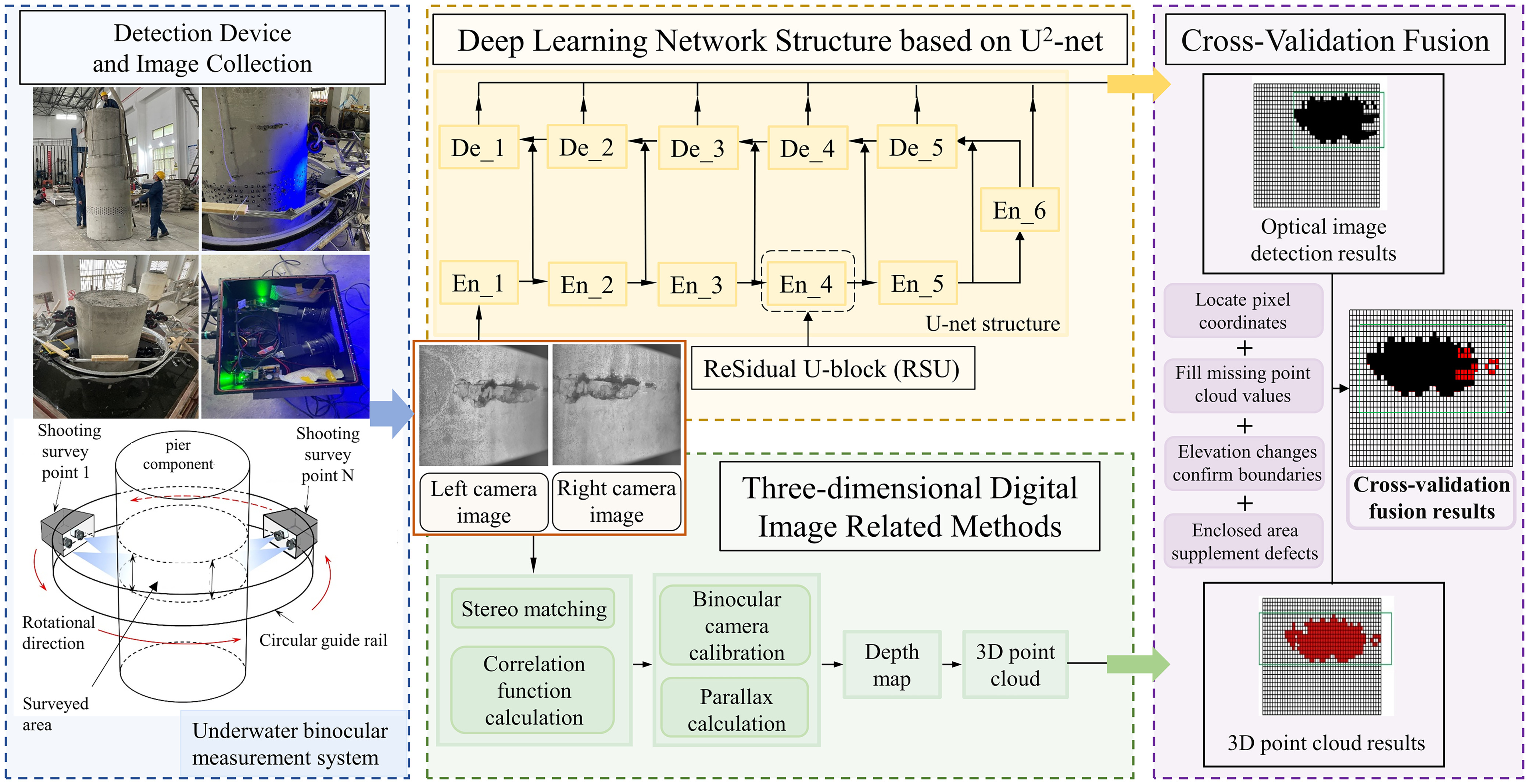
In this work, the innovative defect detection approach that fuses deep learning with 3D point cloud fusion is introduced, encompassing deep learning–based defect recognition, 3D DIC, and their synergistic fusion, as shown in Fig. 1. The methodology involves initially applying deep learning for defect feature extraction and segmentation in images, followed by employing 3D DIC for physical dimension calculations and stereo matching for point cloud generation. Subsequent matching of deep learning–segmented defect regions with point cloud data enables refined defect measurement through the complementary strengths of each technique.

Fig. 1. (Color) Defect detection method research technical route.

Deep Learning–Based Defect Recognition Model

This study utilizes an encoder–decoder structure from deep learning to perform analysis and research on underwater concrete images of bridges by adopting a multilevel nested U-Net structure (Ronneberger et al. 2015), informed by U²-Net (Qin et al. 2020), to achieve accurate defect recognition and segmentation in underwater concrete imagery. This method addresses the shortcomings of prior techniques that achieved deeper architectural layers at the expense of high-resolution feature maps (Zhang et al. 2018; Hou et al. 2022). The method builds upon and refines the designs of traditional fully convolutional networks and U-Net, overcoming prior limitations in semantic segmentation such as low computational efficiency and the incomplete extraction of contextual information.

Image Acquisition and Defect Classification

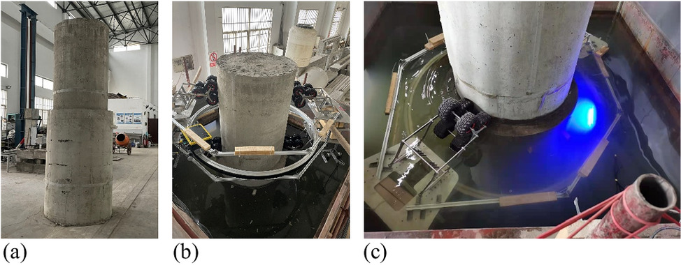
Most publicly available underwater image data sets contain only images and annotation files, lacking the physical dimensions of defects. To validate the effectiveness of the proposed method for measuring physical dimensions, experiments were conducted using a self-constructed data set. To create a training data set for deep learning, a 3 m × 3 m × 3 m water tank was set up in a laboratory to mimic underwater inspection conditions, as shown in Fig. 2. A full-scale, concrete bridge pier with variable cross sections was constructed, incorporating typical structural defects like spalling, exposed rebars, and cracks on surface. Considering the specific nature of underwater structural defects, exposed water pipes were designed to account for voids in pipelines (Teng et al. 2024). Calibration papers were affixed to the pier surface to simulate moss and other vegetation defects (Freire et al. 2015; Potenza et al. 2020; Pushpakumara and Thusitha 2021). For underwater bridge structures, vegetation (mainly moss) growth can cause root systems to penetrate microcracks, further enlarging these cracks, accelerating water infiltration, and damaging the durability of concrete bridges (González-Jorge et al. 2012; Conde et al. 2016). Vegetation growth also obscures the observation of other surface defects (such as cracks). To ensure experimental safety, the number of exposed water pipes was limited to four, resulting in a small sample size. Therefore, vegetation and voids in pipeline defects were combined and collectively termed foreign objects. Similarly, there are only four instances of exposed rebars, which often occur concurrently with spalling. Therefore, exposed rebars and spalling are combined and collectively termed spalling and exposed rebars.

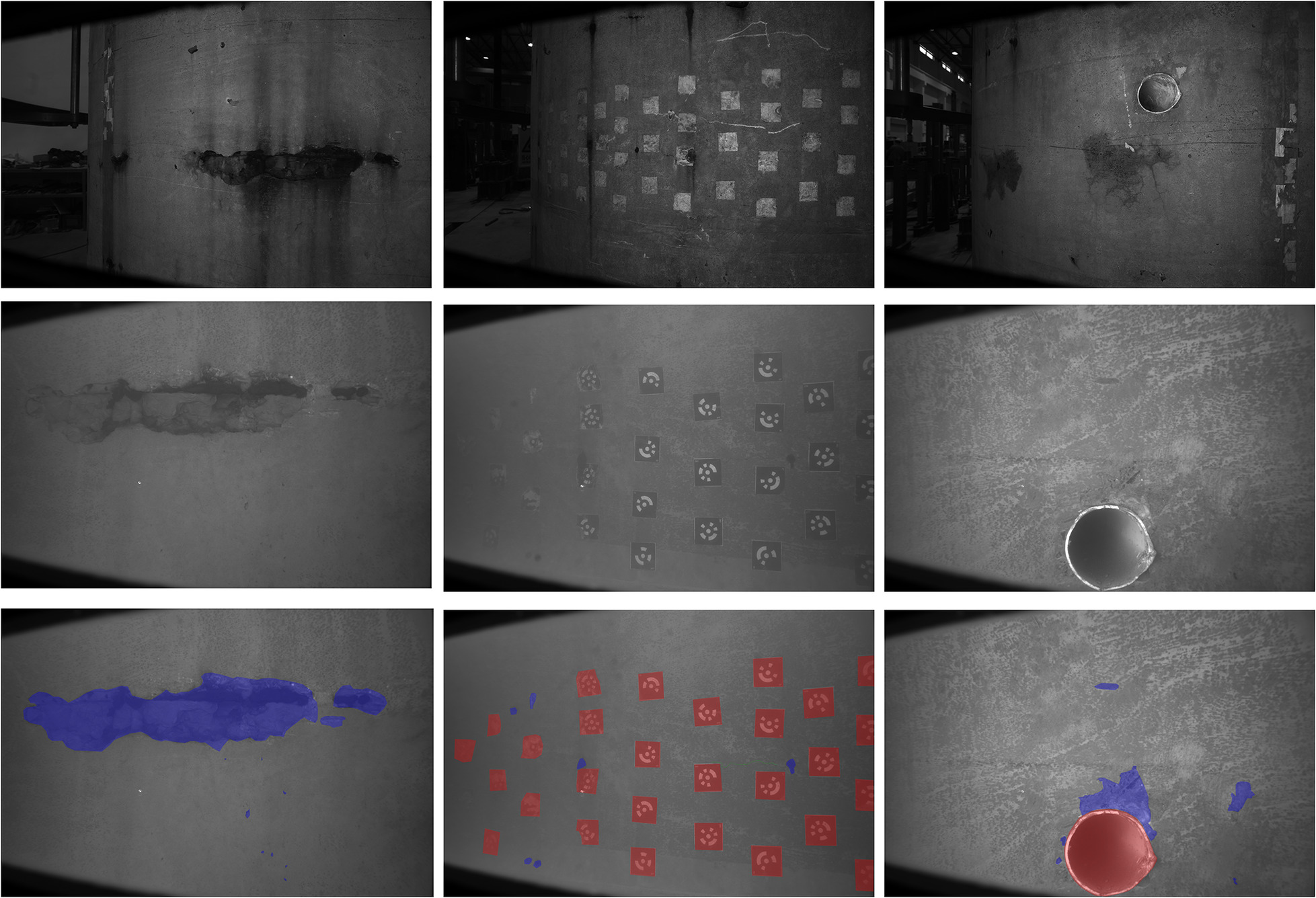
Fig. 2. (Color) Full-scale components and underwater simulation environment: (a) full-scale bridge pier component diagram; (b) underwater environment diagram; and (c) schematic diagram of underwater environment image acquisition process.

To overcome underwater imaging challenges like turbid water, poor lighting, and low resolution, a 20-megapixel complementary metal oxide semiconductor (CMOS) camera (max resolution 5,472 × 3,648) with LED 5050 array lights emitting blue light was employed. Blue light, due to its shorter wavelength, penetrates water better (Chiang and Chen 2012), improving visibility, contrast, and reducing color distortion, consequently enhancing detection accuracy. Fig. 3 illustrates three typical types of defects in the data set. The first row shows defect images taken in air, the second row displays defect images captured underwater, and the third row presents annotated defect images.

U²-Net Neural Network Structure

U²-Net is a novel network architecture based on U-Net, which has shown promising results in foreground–background segmentation tasks with small pixel proportions. The new residual U-blocks (RSU) module based on U-Net is an integral part of our neural network encoder–decoder pairs.

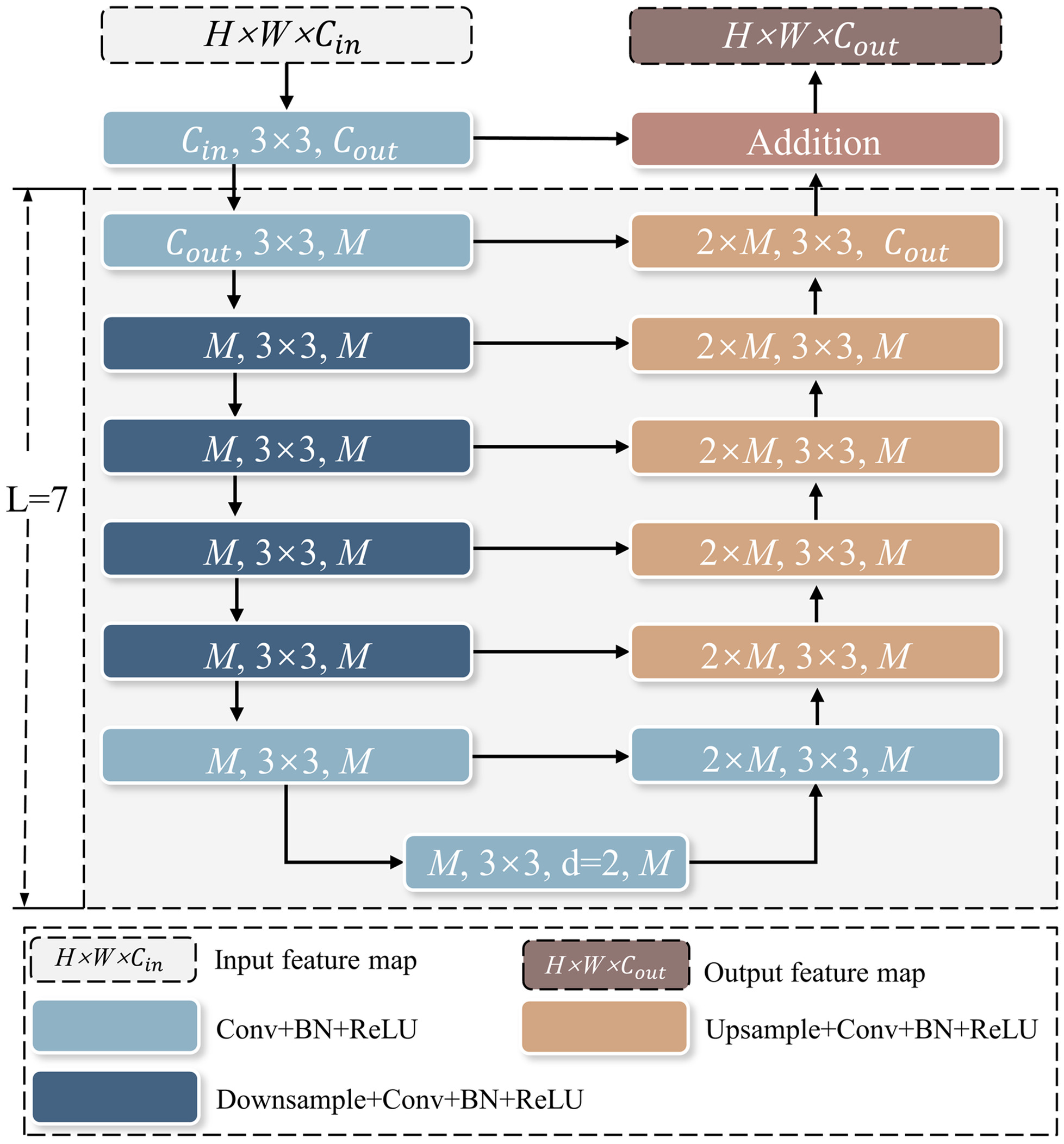
The RSU structure used in U²-Net is mainly used to capture multiscale features within each encoder and decoder. The RSU-L (C_in, M, C_out) structure is shown in Fig. 4, where L is the number of layers in the encoder, C_in and C_out represent the input and output channels, respectively, and M represents the number of channels in the internal layer of RSU. RSU first uses the input convolutional layer to transform the input feature map x (H × W × C) into an intermediate map F₁(x) with channel C_out. Then, a symmetric encoder–decoder structure similar to U-Net, with a height of L, is used to take the intermediate feature map F₁(x) as input to learn to extract and encode multiscale contextual information U[F₁(x)]. A larger L will result in more pooling operations, larger receptive field range, and richer local and global features. Finally, the residual connection of local features and multiscale features is fused by summing F₁(x) + U[F₁(x)]. By adjusting L with different parameters, local features and multiscale features are fused through residual connections to reduce the loss of detail features caused by large-scale upsampling.

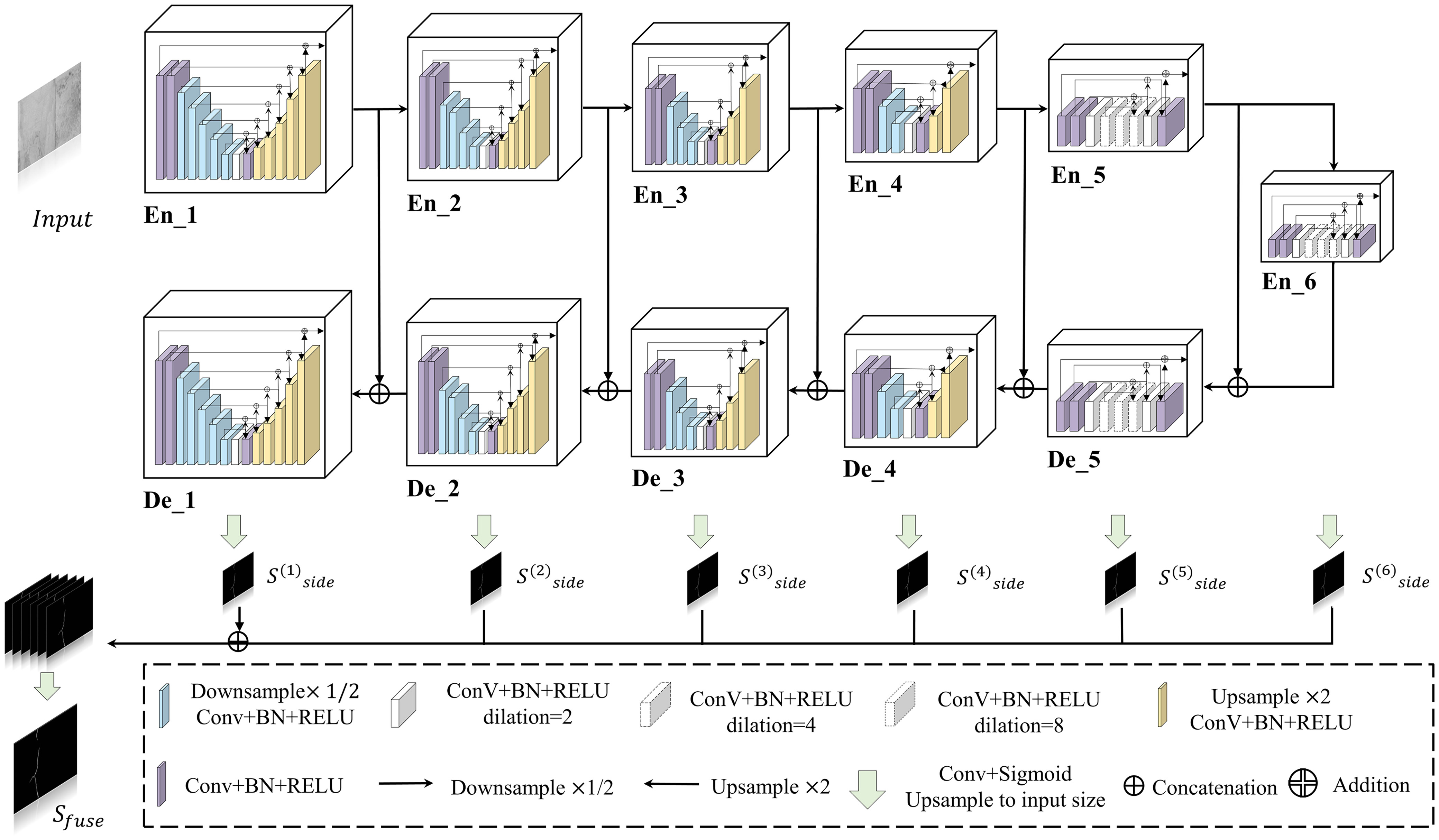
Fig. 4. (Color) RSU schematic diagram of the structure.

As illustrated in Fig. 5, U²-Net structure consists of six encoders, five decoders, and a saliency map fusion module that interlinks them. This multilevel nested U setup enhances the extraction of multiscale features within each pair and facilitates effective feature aggregation across layers. Encoders 1–4 utilize RSU modules of varying heights (L = 7 to 4) to capture features at different scales. According to the spatial resolution of the input feature maps, L is usually configured. For feature maps with large height and width, greater L is used to capture more large-scale information. The resolution of feature maps in Encoders 5 and 6 are relatively low; further downsampling of these feature maps leads to loss of useful context. Hence, Encoders 5 and 6 adopt dilated version RSU modules with a height of 4 to ensure that the intermediate feature maps have the same resolution as the input feature maps. The decoder stages have similar structures to their symmetrical encoder stages. In Decoder 5, the dilated version RSU module with a height of 4 is also used. Each decoder stage takes the concatenation of the upsampled feature maps from its previous stage and those from its symmetrical encoder stage as the input. The last part is the saliency map fusion module, which is used to generate saliency probability maps. U²-Net first generates six side output saliency probability maps, S_{side (6)}, S_{side (5)}, S_{side (4)}, S_{side (3)}, S_{side (2)}, and S_{side (1)}, from the stages of Encoder 6, Decoder 5, Decoder 4, Decoder 3, Decoder 2, and Decoder 1 by a 3 × 3 convolution layer and a sigmoid function. Then, it upsamples these saliency maps to the input image size and fuses them with a concatenation operation followed by a 1 × 1 convolution layer and a sigmoid function to generate the final saliency probability map S_fuse, as shown in Fig. 5. The neural network model based on U²-Net, using RSU blocks, avoids the need for preadjusted pretrained parameters, ensuring flexibility, reduced performance degradation, and suitability for underwater imaging environments.

Fig. 5. (Color) U²-net structure diagram.

Loss Function

In terms of loss function design, the model evaluates not only the output feature maps from the network but also the intermediate fused feature maps. The total loss function L combines weighted losses from multiple side output feature maps and the final feature map, adjusts the weights of cross-entropy loss based on the sample class proportions, and employs the Intersection over Union (IoU) metric as the optimization target for defect segmentation. This approach effectively balances the assessment and optimization needs for multiclassification problems. The formulas are as follows:

L = \sum_{m = 1}^{M} w_{s}^{(m)} l_{s}^{(m)} + w_{f} l_{f}

(1)

CE = - \sum_{i}^{C} t_{i} \log (f {(s)}_{i})

(2)

where

l_{s}^{(m)}

= loss of the six side output feature maps; l_f = loss of the final feature map; and

w_{s}^{(m)}

and w_f = respective weights balancing these two losses. The variable t_i denotes the true value and f(s)i denotes the normalized exponential function value for each category.

Three-Dimensional Point Cloud Reconstruction Based on Three-Dimensional Digital Image Correlation

The reconstruction of 3D morphology of underwater structural surface defects using the 3D DIC method is analogous to aerial 3D reconstruction. By matching the defect edge pixel areas segmented through deep learning with the corresponding positions in the point cloud, the actual physical dimensions of localized defects can be accurately determined, facilitating more precise measurements of these defects.

Principle of Binocular Vision

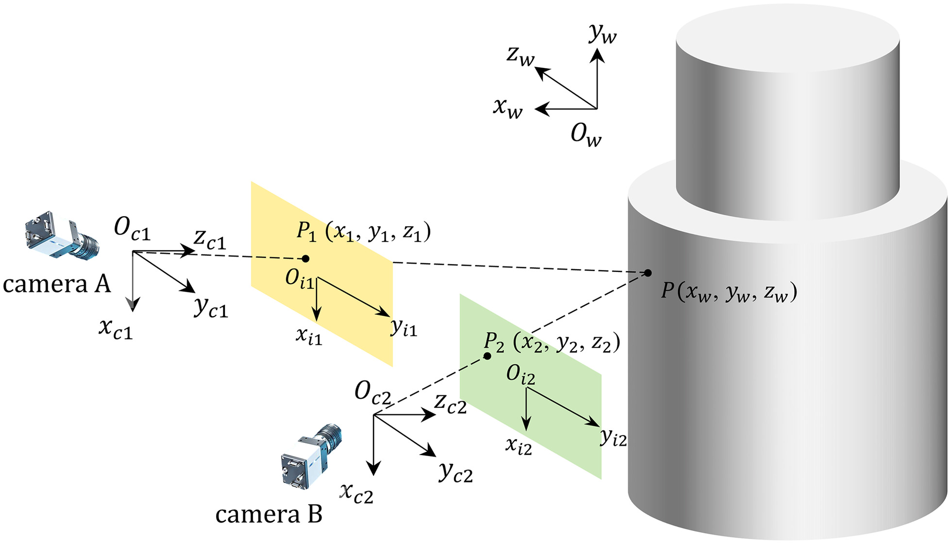
3D digital image correlation measurement is based on the principle of binocular stereovision. Two cameras simultaneously capture images of the same scene from different viewpoints. Corresponding points are then identified in the two 2D images. Using the calibration parameters of the binocular cameras, including the intrinsic and extrinsic parameters and distortion coefficients, the 3D coordinates of the points in the scene can be calculated. As illustrated in Fig. 6, O_w − x_wy_wz_w represents the world coordinate system where the spatial point P(x_w, y_w, z_w) is located. O_c − x_cy_cz_c and O_i − x_iy_iz_i denote the camera coordinate systems and pixel coordinate systems for each camera, respectively. Points P₁(x₁, y₁, z₁) and P₂(x₂, y₂, z₂) are the projections of point P on the image planes of Cameras A and B, respectively. The optical center O_c₁ of Camera A, image point P₁, and spatial point P are collinear, as are the optical center O_c₂ of Camera B, image point P₂, and spatial point P. Therefore, the intersection of lines O_c₁ · P₁ and O_c₂ · P₂ determines the 3D coordinates of point P.

Fig. 6. Principle of binocular stereovision.

Stereo Matching

Stereo matching involves finding corresponding points in the digital images of the object surface recorded by two cameras (Poggi et al. 2021), as shown in Fig. 7. To accurately match image subregions in the left and right views, the selection of shape functions should consider not only the imaging relationship of the cameras but also the height information of the object surface.

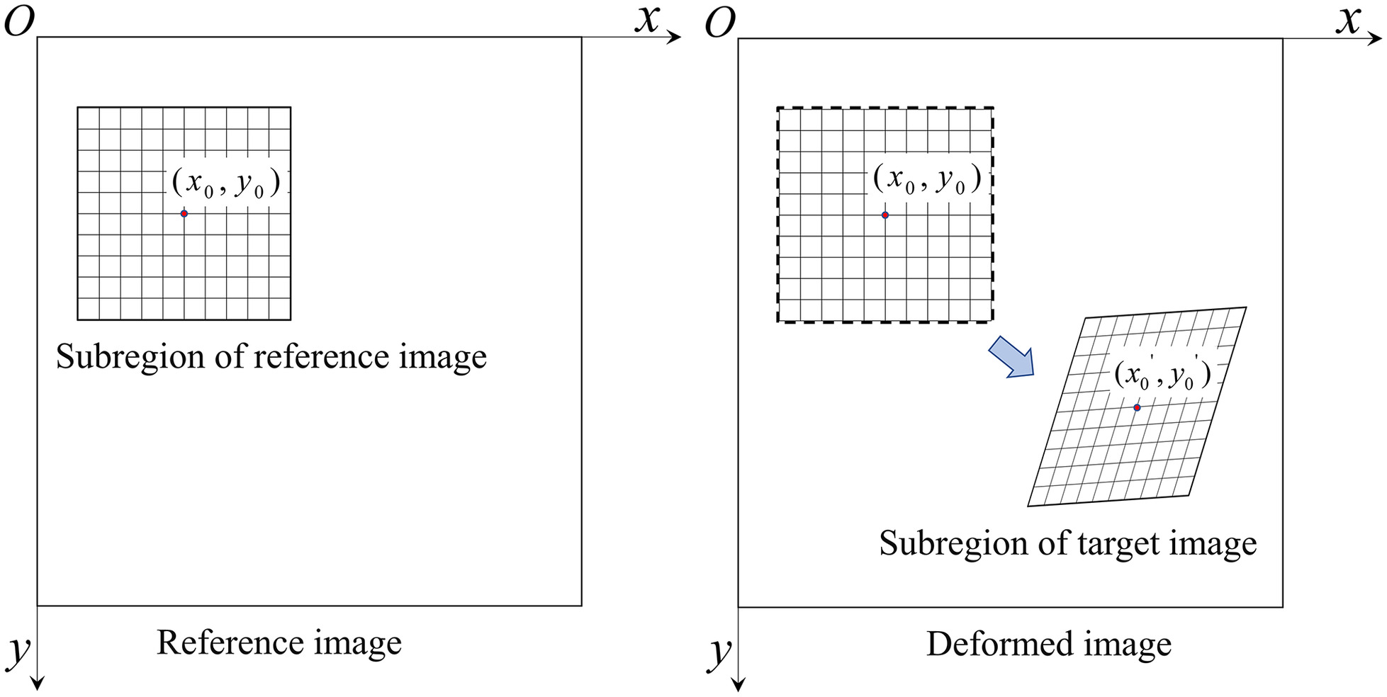
Fig. 7. (Color) Image subregion correlation matching graph.

In this paper, the zone-based stereo matching algorithm was selected. This approach selects a subwindow around a pixel point in one image and searches for the most similar subwindow in the other image based on similarity measures. The matched pixel in the corresponding subimage represents the matching point. Given the zero mean normalized cross-correlation (ZNCC) method’s robustness against illumination changes, it is chosen for computing the disparity map. The matching level between subimages and the template is calculated using a normalized correlation formula, which is defined as follows:

ZNCC = \frac{1}{n} \sum_{x, y} \frac{1}{σ_{f} σ_{t}} (f (x, y) - μ_{f}) (t (x, y) - u_{f})

(3)

where f(x, y) and t(x, y) = two vectors to be compared; n = dimensionality of the vectors or the window size; σ = standard deviation of the two samples; and μ = mean of the two samples.

First, let us designate one image as I1 and the image to be matched as I2, both of size H × W. Then, employing the ZNCC similarity measure formula, a template window size and region T are selected in the left camera image. The template is moved with a specified step size in the right camera image, and the similarity S between the corresponding region and T is calculated, completing one matching calculation. To achieve subpixel image matching and enhance matching accuracy, various nonlinear optimization methods can be utilized for parameter calculation (Bruck et al. 1989; Baker and Matthews 2004). The parameters can be determined based on the correspondence between the same feature point in the left and right images:

x^{'} = x_{0} + δ_{x} + ε_{0} + ε_{x} δ_{x} + ε_{y} δ_{y} + \frac{1}{2} ε_{x x} δ_{x^{2}} + ε_{x y} δ_{x} δ_{y} + \frac{1}{2} ε_{y y} δ_{y^{2}}

(4)

y^{'} = y_{0} + δ_{y} + η_{0} + η_{x} δ_{x} + η_{y} δ_{y} + \frac{1}{2} η_{x x} δ_{x^{2}} + η_{x y} δ_{x} δ_{y} + \frac{1}{2} η_{y y} δ_{y^{2}}

(5)

where x₀ and y₀ = center point of the template region; δ_x = x − x₀; δ_y = y − y₀; ε₀ and η₀ = parallaxes between the center points of the right image and the template region in the left image; ε_x, ε_y, η_x, and η_y = first-order derivatives of the parallaxes within the template; and ε_xx, ε_yy, ε_xy, η_xx, η_yy, and η_xy = second-order derivatives of the parallaxes within the template.

The maximum similarity S in the current matching calculation result is selected as the most matching position. Then, the horizontal distance difference between the left image and the pixel at the most matching position in the image to be matched is computed as the parallax value corresponding to the current pixel.

Three-Dimensional Point Cloud Reconstruction

By calibrating the binocular cameras, the parameters of the camera system are obtained. Using the DIC method, corresponding points in the images from both cameras are accurately matched (Ge et al. 2024). Alongside camera calibration, the stereo cameras establish a spatial world coordinate system based on a calibration template, allowing for the reconstruction of 3D spatial coordinates of interest points. After obtaining the parameters and distortion coefficients of both cameras, the projection matrices M1 and M2 for the left and right cameras can be calculated as follows:

Z_{c 1} [\begin{matrix} u_{1} \\ v_{1} \\ 1 \end{matrix}] = M_{1} [\begin{matrix} x_{w} \\ y_{w} \\ \begin{matrix} z_{w} \\ 1 \end{matrix} \end{matrix}] = [\begin{matrix} \begin{matrix} \begin{matrix} m_{11}^{c 1} & m_{12}^{c 1} \end{matrix} & \begin{matrix} m_{13}^{c 1} & m_{14}^{c 1} \end{matrix} \end{matrix} \\ \begin{matrix} \begin{matrix} m_{21}^{c 1} & m_{22}^{c 1} \end{matrix} & \begin{matrix} m_{23}^{c 1} & m_{24}^{c 1} \end{matrix} \end{matrix} \\ \begin{matrix} \begin{matrix} m_{31}^{c 1} & m_{32}^{c 1} \end{matrix} & \begin{matrix} m_{33}^{c 1} & m_{34}^{c 1} \end{matrix} \end{matrix} \end{matrix}] [\begin{matrix} x_{w} \\ y_{w} \\ \begin{matrix} z_{w} \\ 1 \end{matrix} \end{matrix}]

(6)

Z_{c 2} [\begin{matrix} u_{2} \\ v_{2} \\ 1 \end{matrix}] = M_{2} [\begin{matrix} x_{w} \\ y_{w} \\ \begin{matrix} z_{w} \\ 1 \end{matrix} \end{matrix}] = [\begin{matrix} \begin{matrix} \begin{matrix} m_{11}^{c 2} & m_{12}^{c 2} \end{matrix} & \begin{matrix} m_{13}^{c 2} & m_{14}^{c 2} \end{matrix} \end{matrix} \\ \begin{matrix} \begin{matrix} m_{21}^{c 2} & m_{22}^{c 2} \end{matrix} & \begin{matrix} m_{23}^{c 2} & m_{24}^{c 2} \end{matrix} \end{matrix} \\ \begin{matrix} \begin{matrix} m_{31}^{c 2} & m_{32}^{c 2} \end{matrix} & \begin{matrix} m_{33}^{c 2} & m_{34}^{c 2} \end{matrix} \end{matrix} \end{matrix}] [\begin{matrix} x_{w} \\ y_{w} \\ \begin{matrix} z_{w} \\ 1 \end{matrix} \end{matrix}]

(7)

where (u₁, v₁) and (u₂, v₂) = homogeneous coordinates of a point on the ideal image plane of the object surface in the left and right cameras, respectively; (x_w, y_w, z_w, 1) = homogeneous coordinate of the point in the world coordinate system; and m_ij(i = 1, 2, …, j = 1, 2, …) = element in the ith row and jth column of the projection matrix. By eliminating Z_c₁ and Z_c₂ from the aforementioned two equations, the following four linear equations regarding the spatial coordinates (x_w, y_w, z_w, 1) were obtained:

\begin{aligned} (u_{1} m_{31}^{c 1} - m_{11}^{c 1}) x_{w} & + (u_{1} m_{32}^{c 1} - m_{12}^{c 1}) y_{w} + (u_{1} m_{33}^{c 1} - m_{13}^{c 1}) z_{w} \\ = m_{14}^{c 1} - u_{1} m_{34}^{c 1} \end{aligned}

(8)

\begin{aligned} (v_{1} m_{31}^{c 1} - m_{21}^{c 1}) x_{w} & + (v_{1} m_{32}^{c 1} - m_{22}^{c 1}) y_{w} + (v_{1} m_{33}^{c 1} - m_{23}^{c 1}) z_{w} \\ = m_{24}^{c 1} - v_{1} m_{34}^{c 1} \end{aligned}

(9)

\begin{aligned} (u_{2} m_{31}^{c 2} - m_{11}^{c 2}) x_{w} & + (u_{2} m_{32}^{c 2} - m_{12}^{c 2}) y_{w} + (u_{2} m_{33}^{c 2} - m_{13}^{c 2}) z_{w} \\ = m_{14}^{c 2} - u_{2} m_{34}^{c 2} \end{aligned}

(10)

\begin{aligned} (v_{2} m_{31}^{c 2} - m_{21}^{c 2}) x_{w} & + (v_{2} m_{32}^{c 2} - m_{22}^{c 2}) y_{w} + (v_{2} m_{33}^{c 2} - m_{23}^{c 2}) z_{w} \\ = m_{24}^{c 1} - v_{2} m_{34}^{c 2} \end{aligned}

(11)

From the aforementioned equations, an overdetermined equation is formed. Due to the inevitable presence of noise in the actual data, the least squares method is employed to compute the three-dimensional coordinates of the spatial points. By repeating the aforementioned process for all matched point pairs in the reference images, the spatial coordinates of points on the surface of the measured area can be obtained, thus yielding the three-dimensional point cloud of the measured object’s surface.

Structural Surface Defect Measurement Based on Fusion of Semantic Segmentation and 3D Point Cloud

After segmenting underwater image-based defects using deep learning models, calculating the actual physical dimensions of pathologies from segmented image edges becomes necessary. For above-water structural inspections, methods like laser ranging or affixing markers on surfaces to map pixels to physical dimensions are common. However, these approaches are not feasible underwater. Instead, a binocular stereovision–based method is employed for mapping pixels to their physical dimensions.

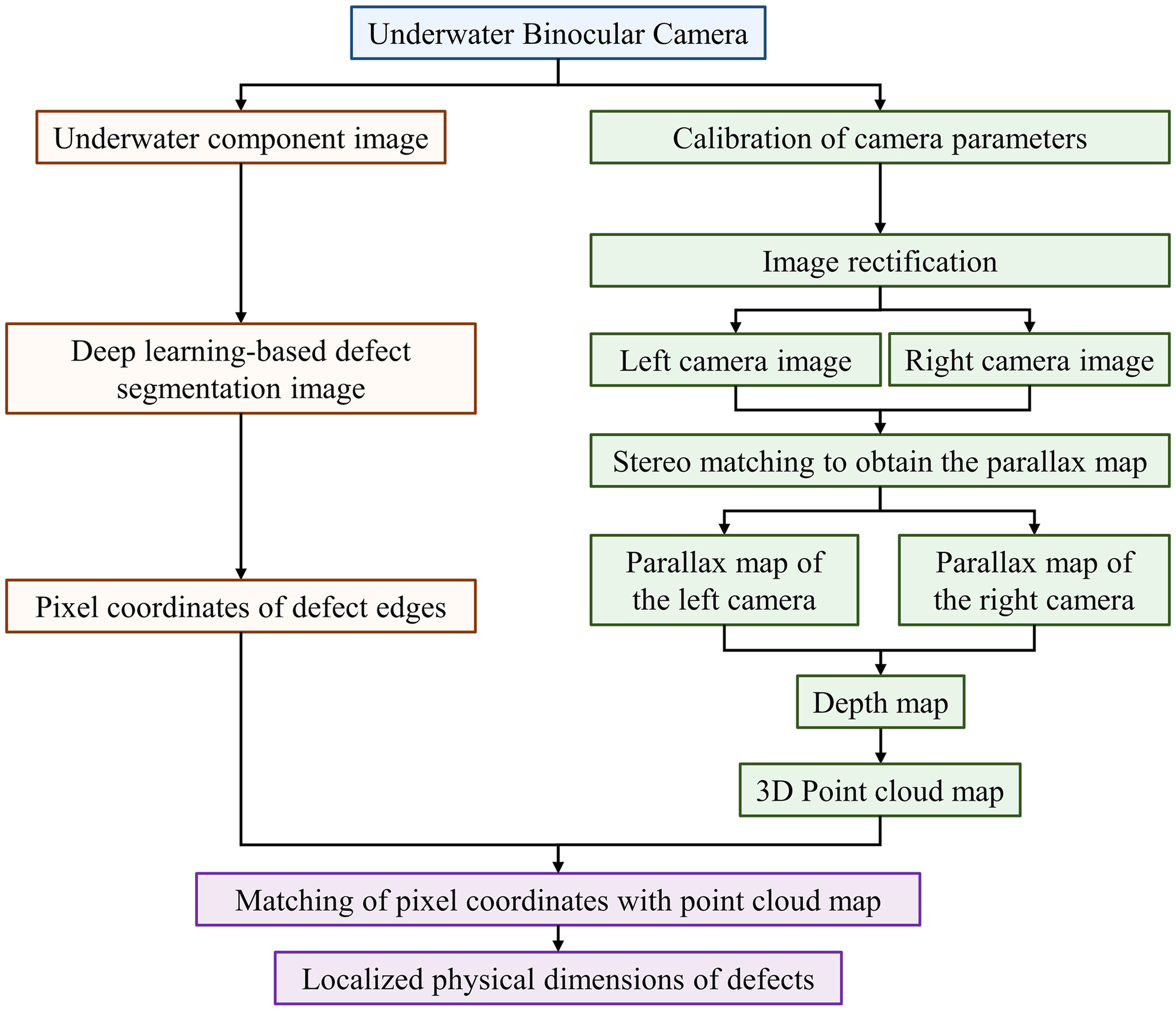
Once the correspondence between three-dimensional space and the image is established, stereo matching techniques clarify the relationship between points in the left and right images, enabling parallax calculation and recovery of three-dimensional point information. This process involves underwater binocular camera calibration, image rectification, stereo matching, and the computation of depth and point cloud. The physical dimensions of localized pathologies are obtained by matching the deep learning–segmented edge pixels with their corresponding positions in the point cloud, as outlined in Fig. 8. The binocular camera’s intrinsic parameters are calculated using Zhang’s chessboard calibration method (Chen and Pan 2020). Image rectification includes epipolar correction and distortion correction, aligning the pixels row-wise across both camera images. The binocular parallel rectification aligns camera coordinate systems with the world coordinate system, followed by epipolar alignment using rotation matrices R1 and R2, and distortion correction. Finally, the camera coordinate system is converted back to pixel coordinates using the intrinsic matrix, with pixel values from the original coordinates assigned to the new image coordinates.

Fig. 8. (Color) Localized defect measurement based on binocular stereovision flow chart.

The parallax map of the entire image is obtained through stereo matching, and then the actual depth map is calculated using the following formula:

depth = \frac{f_{c} \times D_{c_{1} c_{2}}}{disp}

(12)

where depth = depth value; f_c = normalized focal length of the intrinsic parameters;

D_{c_{1} c_{2}}

= distance between the optical centers of the binocular cameras; and disp = parallax.

Therefore, the point cloud coordinates of each pixel are calculated as follows:

z = \frac{d}{s} x = \frac{(u - C_{x}) \times z}{f_{x}} y = \frac{(v - C_{y}) \times z}{f_{y}}

(13)

where u and v = image pixel coordinates; s = camera scaling factor; and f_x, f_y, C_x, and C_y = calibrated camera intrinsic parameters.

Upon acquiring point cloud data, the coordinates for each pixel’s corresponding point in the cloud are known. By using deep learning models to identify the coordinates of pixels at the edges of lesions, the spatial three-dimensional coordinates of these edge pixels within the point cloud can be found. Projecting these coordinates onto the image plane allows us to delineate the polygonal areas of pathology formed by point cloud data on this plane, as depicted in Fig. 9. Based on the Shoelace theorem (Braden 1986), given the vertices’ coordinates, the area of any polygon can be calculated as follows:

S = \frac{1}{2} | \sum_{i = 1}^{n} (x_{i} y_{i + 1} - x_{i + 1} y_{i}) |, x_{n + 1} = x_{1}, y_{n + 1} = y_{1}

(14)

where x and y = pixel coordinates on the image plane.

Fig. 9. (Color) Mapping diagram of image segmentation results and point cloud reconstruction results.

Experimental Results Analysis

In the full-scale bridge pier components fabricated under laboratory conditions, defects such as cracks, spalling, exposed rebars, and foreign objects were designed. A total of 1,734 underwater component images were collected in the laboratory. The data set samples were randomly split into training, validation, and test sets at a ratio of 8:1:1. The Adam optimization algorithm was chosen for model training with a learning rate of 0.0001 over 70 total epochs, adjusting the learning rate to 95% of the previous step at epochs 10, 20, 30, 40, and 50. To validate the model’s effectiveness, the original U-Net network structure was employed for comparison. The analysis of existing underwater image data revealed a ratio of 15 (exposed rebars): 368 (spalling and exposed rebars) samples, with only 4 effective samples. Specifically, there are four instances of exposed rebars on the bridge piers, with 15 images depicting exposed rebars and 368 images showing spalling and exposed rebars. Considering the shortage of exposed rebar samples and the fact that exposed rebar often co-occurs with spalling, both were treated as the same detection category, resulting in three practical detection categories: cracks, spalling and exposed rebars, and foreign objects.

Defect Segmentation Results

Considering the limited sample data for crack defects and the high resolution of the imaging equipment used in this study, a sliding window strategy was employed to augment the collected image data set. The sliding window size was set at 544 × 544 pixels, with a stride of 256, resulting in 1,157 crack training images. The data set also included 368 samples of spalling and exposed rebar images, with minimum and maximum bounding box sizes ranging from 3 × 3 to 1,928 × 1,652 pixels, indicating a wide variation in target sizes. To detect small targets and accommodate the semantic needs of larger objects, the network input size was increased to 1,024 × 1,024. The training data for the spalling and exposed rebars category were generated using a window size equal to half the original dimensions of the images, without considering overlap, producing 1,146 samples. Additionally, 180 foreign object samples were processed similarly, with an average effective foreground pixel ratio of 0.0986, yielding 465 samples. The number of data set samples is presented in Table 1.

Table 1. Number of defects in the data set

Category	Original number	Expanded number
Spalling and exposed rebars	368	1,146
Foreign object	180	465
Crack	109	1,157

Table 2 presents the final test comparison results between two groups of models. The data indicate that both model groups exhibit good predictive performance for detecting foreign objects and spalling and exposed rebars, with U²-Net achieving pixel accuracy rates of 0.943 for foreign objects and 0.811 for spalling and exposed rebars. In terms of IoU comparisons for segmentation results, U²-Net significantly outperforms with scores of 0.733 for foreign objects and 0.411 for spalling and exposed rebars, reaching a mean intersection over union (mIoU) of 0.548. U-Net, however, shows weaker performance in IoU, with an mIoU of only 0.503. Nevertheless, both models underperform in crack detection due to the extremely low proportion of crack pixels as foreground targets against the background, accounting for just 0.464%, leading to poor detection results. This issue is primarily attributed to the high difficulty of observing cracks underwater, influenced by surrounding features and the limited size of sample populations. Errors in manual annotation, inconsistent labeling standards, and the small scale of crack samples contribute to the inferior results for crack detection.

Table 2. Comparison of U²-net and U-net indicators

Category	Metric	Model
Category	Metric	U²-Net	U-Net
Background	Recall	0.999	0.999
	PA	0.992	0.987
	IoU	0.991	0.986
Crack	Recall	0.272	0.193
	PA	0.151	0.121
	IoU	0.093	0.056
Foreign object	Recall	0.876	0.720
	PA	0.943	0.958
	IoU	0.733	0.609
Spalling and exposed rebars	Recall	0.466	0.352
	PA	0.811	0.854
	IoU	0.411	0.325
mIoU (c)		0.548	0.503
mIoU		0.711	0.640

Note: (c) = The mean IoU that includes cracks; and PA = Pixel accuracy.

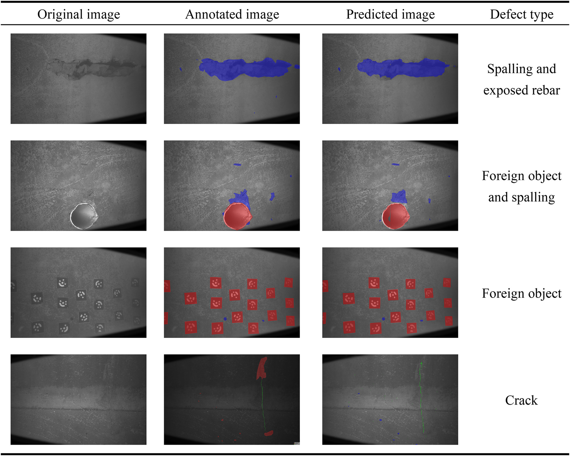
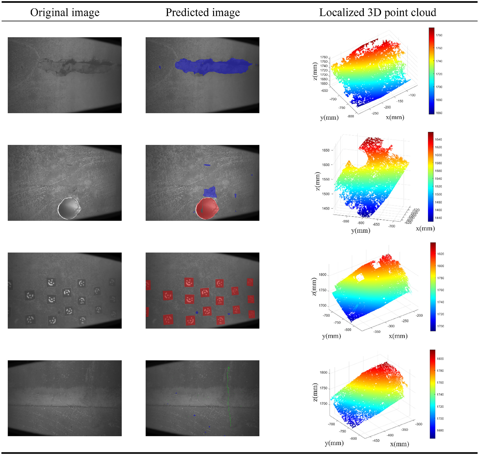
To evaluate the performance and segmentation effects of the U²-Net model, this study selected several representative images based on defect type, distribution location, and defect area size, as shown in Fig. 10. The results indicate that the model based on U²-Net proposed in this study successfully identifies various types of defect information in underwater images, extracting defect category and distribution location from images taken from two angles by left and right cameras. The model was trained with images including two types of foreign objects, which could be accurately segmented owing to their distinct features on the concrete surface. Moreover, the model precisely located and segmented large-area defects at different positions and recognized small-area defects effectively, although the segmentation accuracy for small defects was poorer compared to large-area defects, and there were some variations in segmentation results for the same defect from different angles. Additionally, the model can recognize multiple types of information simultaneously through the underwater defect segmentation inference process. In terms of crack detection, the model effectively detects long cracks due to the quantity of crack samples but performs poorly in recognizing and segmenting fine cracks and similar defects, resulting in some misjudgments.

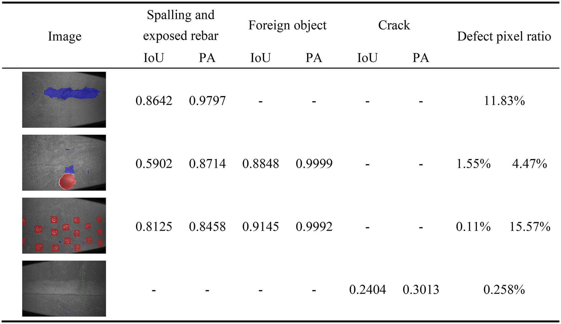
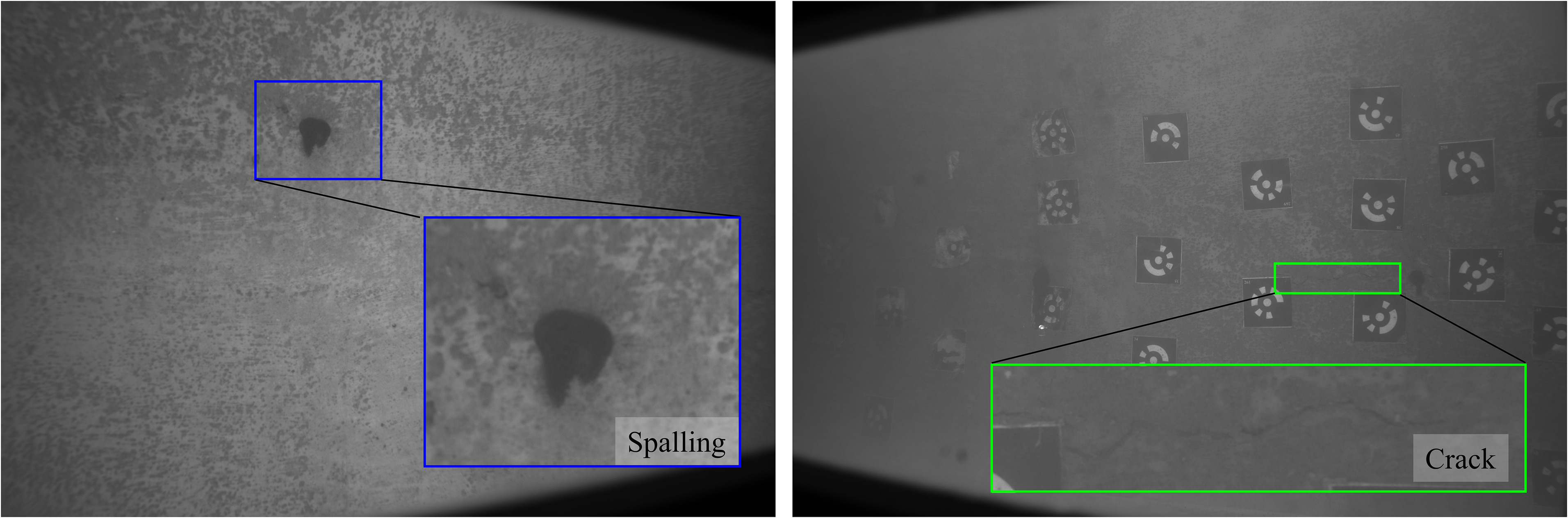
The results of defect segmentation are presented in Fig. 11. The highest recognition accuracy was observed for foreign objects, with a segmentation accuracy (IoU) for large-area defects reaching 0.8642. By contrast, smaller defects exhibited an IoU of approximately 0.6. The IoU for cracks was only 0.2404, which, relative to the resolution of the entire image at 3,648 × 5,472, accounts for a mere 0.258% of predicted crack pixels. This is primarily because of the limited number of training samples for underwater crack defects. Taking spalling defects as an example, the pixel proportion in the third row of Fig. 11 is only 0.11%. However, analysis of spalling defect characteristics reveals that they mainly manifest as continuous black areas. As shown in Fig. 12, compared to the slender nature of cracks, the characteristics of spalling are more easily distinguished from the surrounding texture features. Thus, further research is necessary for the precise recognition of minor surface cracks in components.

Fig. 11. (Color) Test image metrics results.

Fig. 12. (Color) Comparison of spalling and crack characteristics.

Defect Three-Dimensional Point Cloud Measurement Results

The point cloud reconstruction results, as shown in Fig. 13, indicate partial completeness due to the weak texture features of concrete surfaces. While large-area defects’ point cloud accurately depicts contour information, regions with significant surface undulations cannot be reconstructed due to the limited depth of field of binocular cameras. The reconstructed areas offer more precise contour information compared to defect detection results. The point cloud reconstructions of foreign object defects match the defect detection outcomes, achieving high measurement accuracy and distinct separation from other surface areas. This allows for the calculation of foreign object areas through the one-to-one correspondence between point clouds and image pixels. However, for minor defects such as cracks, the point cloud results are not as discernible, with fine cracks potentially obscured by point cloud interpolation, preventing accurate measurement of crack dimensions. Hence, further research into precise recognition of minor surface cracks is warranted.

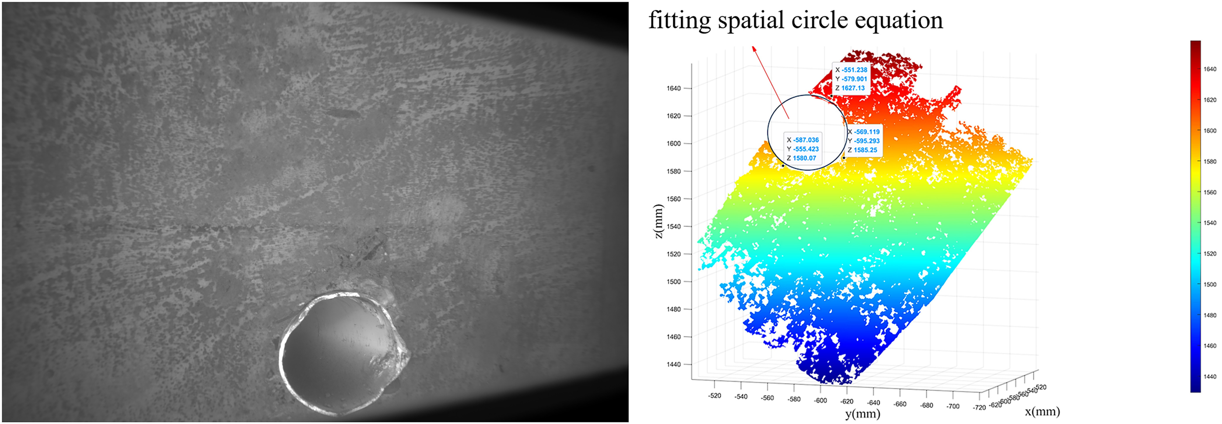
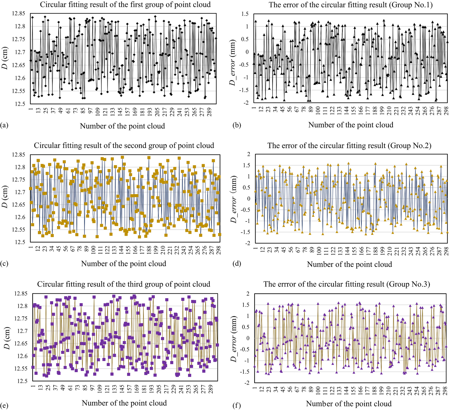
Fig. 13. (Color) 3D point cloud reconstruction results of corresponding defect images.

The experimental results show that the point cloud reconstruction accuracy error of large-area defects is at the millimeter level. Taking the measurement of foreign objects as an example, the diameter of a roughly circular exposed water pipe opening on a concrete bridge pier was measured prior to the experiment, with an inherent manufacturing error. Based on multiple measurements, the average diameter was calculated to be 12.7 cm. As shown in Fig. 14, 900 points were selected along the circumference of the pipe opening’s point cloud morphology and divided into three groups for spatial circle fitting. The fitted diameters of the three circles were 12.7132, 12.7516, and 12.5497 cm, respectively. The diameter for each point was taken as twice the distance from the point to the center of the fitted circle. Fig. 15 illustrates the diameter size corresponding to each point and the respective diameter error, where D represents the diameter. The maximum value of the average diameter error was 1.837 mm, and the standard deviations were 0.8121, 0.9357, and 1.0461 mm, respectively. The analysis suggests that although the 3D DIC–based point cloud reconstruction is limited by the depth of field of the binocular camera, preventing the whole area of defect reconstruction, it demonstrates significant advantages in accurately locating defect edges or contours, achieving excellent measurement precision.

Fig. 14. (Color) Schematic diagram of point cloud screening.

Fig. 15. (Color) Analysis of 3D point cloud measurement results of the foreign object: (a) the first group point cloud circular fit diameter; (b) error of the first group; (c) the second group point cloud circular fit diameter; (d) error of the second group; (e) the third group point cloud circular fit diameter; and (f) error of the third group.

Analysis of Localized Defect Measurement Results by Fusion of Segmentation Results and Point Cloud Information

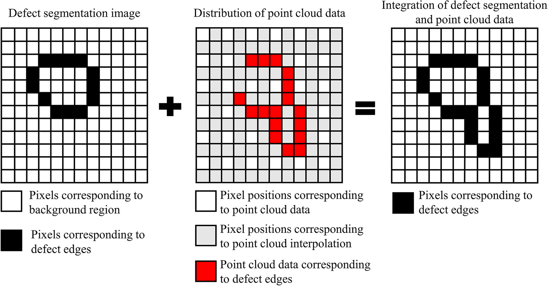
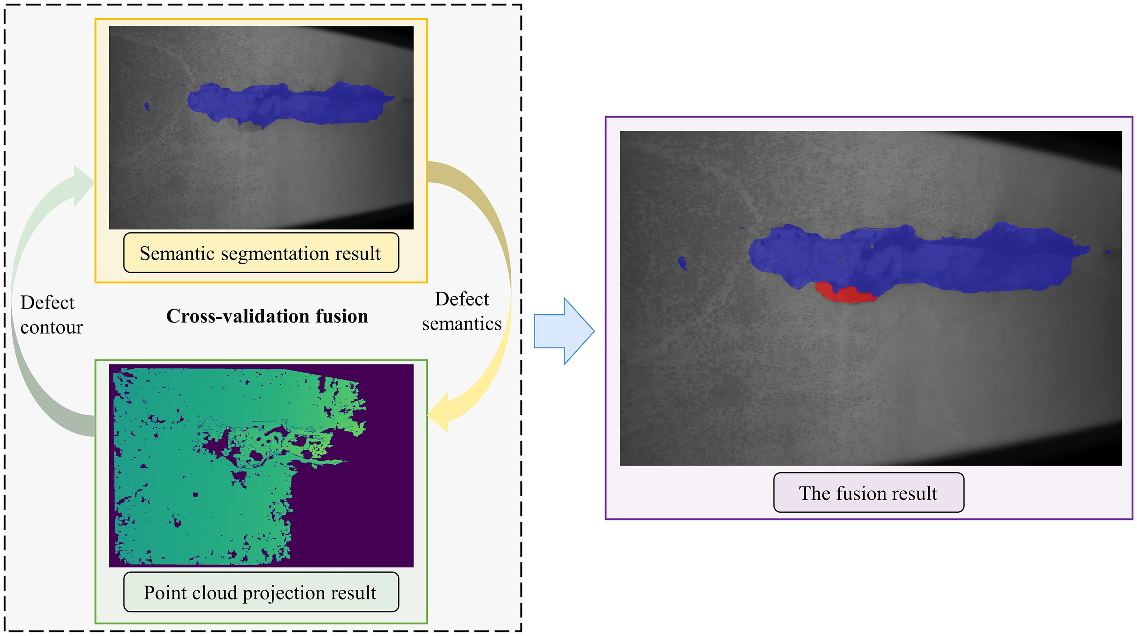
Upon obtaining the segmentation results of the defects, a quantitative measurement of the defects listed in the figure was performed using a stereovision-based measurement method. Due to the precision of matching calculations, the initial point cloud data contain some voids, including unsolved null values and defect areas. To accurately identify defect information in the point cloud, it can be discerned based on the results of deep learning segmentation. Moreover, the segmentation results reveal localized errors in the pixel distribution of the segmented defect areas, with some pixels misclassified as background or defect. Now, by fusing both, further accurate segmentation and measurement of defect locations are achieved, that is, obtaining the actual defect locations from the deep learning model’s segmentation results and correcting the segmentation results through the point cloud values of that area, ultimately calculating the actual defect plane dimensions from the corresponding point cloud data post fusion. Therefore, taking the defect images obtained and calculated from the aforementioned experiments as examples, the following process implements precise measurement of defects:

1.

Based on the deep learning segmentation results, locate the defect areas in the image by obtaining the pixel coordinates of the defect boundaries.

2.

Further refine the deep learning segmentation results by adding missing defect pixels within the closed areas formed by the existing point cloud. Next, use the elevation change data from the point cloud to delineate the pixel boundaries between defective and intact areas, and remove misjudged background areas accordingly.

3.

For the missing parts of the point cloud, based on the segmentation results of the deep learning model, the missing point cloud values corresponding to the edge pixel sequences are filled in with neighboring values.

4.

Based on the fused defect area position, calculate the specific size of the defect using the point cloud coordinate values. According to the aforementioned fusion criteria and process, the final recognition results of the defect image are shown in Fig. 16. Based on Eq. (14), the defect area of the plane projection area is calculated as 105.68 cm².

Fig. 16. (Color) Fusion results of defect segmentation and 3D point cloud.

Conclusions

Accurate identification and quantification of surface defects in underwater bridge structures are of great significance for understanding the structural damage of these underwater components. This paper proposes a method for precise and intelligent detection of defects in underwater bridge substructures, fusing deep learning with 3D point cloud. It proposes a method for identifying surface defects of underwater structures using the U²-Net neural network architecture and for reconstructing localized defects using 3D point cloud. By fusing deep learning semantic segmentation results with 3D point cloud reconstructions, it achieves refined quantitative recognition of localized defects on the surfaces of underwater bridge components.

The neural network model based on U²-Net can effectively identify defects at different locations, including those at the edge of the image or with low resolution. By correcting the elevation changes in the point cloud, the method can more accurately segment large-area defects and also effectively identify smaller defects. It achieves pixel accuracies of 0.943 for foreign objects and 0.811 for spalling and exposed rebars, and IoUs of 0.733 and 0.411, respectively. In addition, the physical size of the defect, including length and area, can be accurately measured through the principle of binocular vision, with an accuracy of up to millimeter level. After combining with the segmentation results, the semantic information of the defect can be accurately obtained.

Although this study presents promising results for intelligent detection and physical dimension measurement of surface defects of underwater bridge structures, several unresolved issues merit attention in future research. First, considering that water quality is often turbid and contains impurities during actual engineering inspections, future research should further investigate detection effectiveness under various water turbidity levels to validate the robustness of the proposed method. Second, the deep learning model should be further improved to enhance its ability to identify and segment subtle defects. Finally, the underwater imaging model needs improvement to account for multiple reflections and refractions of underwater light, to more accurately restore point cloud depth information and reduce distortion.

Data Availability Statement

Some or all data, models, or codes that support the findings of this study are available from the corresponding author upon reasonable request.

Acknowledgments

The research was financially supported by the National Natural Science Foundation of China (52127813 and 52208306), the Natural Science Foundation of Jiangsu Province (BK20220849), and the Jiangsu Provincial Key Research and Development Program (BE2022820).

References

Abdallah, A. M., R. A. Atadero, and M. E. Ozbek. 2022. “A state-of-the-art review of bridge inspection planning: Current situation and future needs.” J. Bridge Eng. 27 (2): 03121001. https://doi.org/10.1061/(ASCE)BE.1943-5592.0001812.

Abstract

Introduction

Methodology

Deep Learning–Based Defect Recognition Model

Image Acquisition and Defect Classification

U2-Net Neural Network Structure

Loss Function

Three-Dimensional Point Cloud Reconstruction Based on Three-Dimensional Digital Image Correlation

Principle of Binocular Vision

Stereo Matching

Three-Dimensional Point Cloud Reconstruction

Structural Surface Defect Measurement Based on Fusion of Semantic Segmentation and 3D Point Cloud

Experimental Results Analysis

Defect Segmentation Results

Defect Three-Dimensional Point Cloud Measurement Results

Analysis of Localized Defect Measurement Results by Fusion of Segmentation Results and Point Cloud Information

Conclusions

Data Availability Statement

Acknowledgments

References

Information

Published In

Copyright

History

Authors

Affiliations

Metrics

Citations

Download citation

Figures

Other

Share

Copy the content Link

Share with email

Share

Request Username

Create a new account

Change Password

Password Changed Successfully

Verify Phone

Congrats!

U²-Net Neural Network Structure