Application of a Closed-Form Analytical Solution to Model Overland Flow and Sediment Transport Using Rainfall Simulator Data

Martins, Matheus Marques; da Costa Lemos, Moisés Antônio; Cavalcante, André Luís Brasil; da Luz, Marta Pereira; Merabet Júnior, José Carlos Frazão; dos Anjos Mascarenha, Márcia Maria

doi:10.1061/IJGNAI.GMENG-9031

Open access

Technical Papers

Jul 9, 2024

Application of a Closed-Form Analytical Solution to Model Overland Flow and Sediment Transport Using Rainfall Simulator Data

Authors: Matheus Marques Martins, Moisés Antônio da Costa Lemos https://orcid.org/0000-0001-9326-7799, André Luís Brasil Cavalcante https://orcid.org/0000-0003-4980-1450 [email protected], Marta Pereira da Luz, José Carlos Frazão Merabet Júnior https://orcid.org/0000-0002-1215-8310, and Márcia Maria dos Anjos MascarenhaAuthor Affiliations

Publication: International Journal of Geomechanics

Volume 24, Issue 9

https://doi.org/10.1061/IJGNAI.GMENG-9031

PDF

Abstract

Rainfall erosion can cause environmental and economic damage by decreasing the storage capacity of water reservoirs because of the detachment of soil particles. The purpose of this study was to develop a one-dimensional physicomathematical model that can help predict the effects of rainfall erosion on the banks of water reservoirs. The model was developed using the Mein–Larson model to describe water infiltration, the kinematic wave approximation to represent overland flow generation, and the steady state sediment continuity equation to estimate sediment transport. The model was validated using rainfall simulator tests and lateritic soil samples with a bimodal soil–water retention curve. The results showed conformity with the experimental data, identifying a threshold in the models for discharge per unit area and sediment yield rate, as well as a linear increase in the models for total runoff and sediment load per unit area. However, the model failed to capture the peak in sediment yield rate owing to raindrop impact during the initial minutes of rainfall. Parametric analysis highlighted the impact of increasing the calibration constant of splash erosion, erodibility coefficient, and critical shear stress on the slope of the sediment load per unit area model. Despite its limitations, the model demonstrates satisfactory predictive capability for sediment load per unit area under high-intensity rainfalls, achieving an R² greater than 0.92 in five of the six cases examined.

Introduction

Erosion processes occurring in watersheds and water reservoir banks can result in sediment deposition in the reservoir, leading to a decrease in its storage capacity and causing various issues, such as reduced electricity production, turbine damage, and operational difficulties with water intake, discharge valves, and gates (Eletrobras 2003). While the behavior of reservoir levels over time is clearly correlated with the water consumption, other factors, such as precipitation, infiltration rate, and geology also play a significant role in this behavior (da Luz et al. 2022). Therefore, understanding and predicting erosion processes in water reservoir areas can facilitate the establishment of preventive measures aimed at reducing these issues.

Water-induced soil erosion involves three main processes: detachment, transportation, and deposition. Detachment is the process of particles being removed from the flow bed because of the shear force of the overland flow and raindrop impact, according to Kinnell (2021). When the detached material is carried away from the site of detachment, transportation occurs, while deposition occurs when the sediment yield rate exceeds the sediment transport capacity of the flow. Sediment discharge can be influenced by a variety of factors, including hydraulic properties of the flow, physical soil properties, and surface characteristics, as discussed by Aksoy and Kavvas (2005).

The steady-state sediment continuity equation forms the basis of the approach to predict erosion across both rill and interrill regions (Nearing et al. 1989). Specifically, rill erosion is considered the phenomenon that arises when the shear force exerted by the water flow surpasses the critical shear stress, a measure of the soil surface's resistance to erosion (Foster and Meyer 1972; Flanagan and Nearing 1995). The erodibility coefficient is used to quantify the ease of the rill erosion (Govindaraju 1998). Interrill erosion, conversely, is mainly caused by the energy of raindrops hitting the soil surface (Fernández-Raga et al. 2017). When the rainfall is evenly distributed, the amount of interrill erosion is directly proportional to the square of the rainfall intensity (Bennett 1974).

Water and temperature movement in both directions is involved in the interaction between soil and atmosphere. Moisture content and soil suction changes can affect the water infiltration and overland flow generation (Fredlund and Rahardjo 1993). Rainfall infiltrates the soil surface until the soil's capacity is reached, and any excess of rainfall flows above the soil surface as overland flow. In arid and semiarid regions with low vegetation cover (Agnese et al. 2014), short-duration, high-intensity rainfalls generate an infiltration excess mechanism (Horton 1933, 1937). The Heber Green and Ampt (1911) model assumes that the infiltration begins when a ponding condition forms on the soil surface, separating an upper saturated zone and a lower unsaturated zone. Mein and Larson (1973) expanded the model to include the infiltration before ponding. The infiltration rate is influenced by several factors, including the presence of vegetation cover, slope angle, state of surface compaction, moisture content of the underlying material, saturation ratio, and presence or absence of an air phase, according to Blight (1997).

Physics-based mathematical models are commonly used to predict soil loss during rainfall (Tao et al. 2018). These models utilize the water-continuity equation and the equation of motion, also known as the Saint-Venant equations, to describe the process of overland flow generation. However, finding exact solutions for these complex equations is difficult owing to their high nonlinearity (Wang et al. 2006). As a result, approximate forms are used without compromising the accuracy of the results. The kinematic wave is the dominant wave in overland flow, particularly during the rising part of the hydrograph and much of the recession part (Singh 2002). The kinematic wave model, which assumes the equivalence of friction forces and gravitational forces, can be used to omit the acceleration terms and pressure gradient term from the equation of motion (Henderson and Wooding 1964). This model has been widely used in the literature to study the rainfall-runoff-erosion process (Smith 1976; Parlange et al. 1981; Govindaraju et al. 1990; Sander et al. 1990; Singh 2002; Baiamonte and Agnese 2010; Baiamonte and Singh 2016; Tao et al. 2018, 2023; Su and Zhang 2022).

The steady-state sediment continuity equation can be used to predict interrill erosion by relating it to the rainfall intensity. To determine the calibration constant in this equation, experimental data obtained using a rainfall simulator (RS) must be retro analyzed. The RS is a device used to study the interactions between the rainfall, runoff, and erosion processes (Mendes et al. 2021). To satisfactorily reproduce in situ conditions in the RS, it must be designed to match factors, such as rainfall intensity, spatial uniformity, raindrop size, velocity, kinetic energy, moisture content, soil type and thickness, vegetation cover, and slope (Aksoy et al. 2012; Mendes et al. 2020). The erodibility coefficient and critical shear stress can be estimated using empirical methods, such as the Inderbitzen (1961) test, but this test is not standardized.

To better understand and quantify the process of soil erosion caused by rainfall, this study presents a closed-form analytical solution that can estimate the amount of soil detachment under uniform rainfall conditions. The model is valid for both unimodal and bimodal soils. Unimodal soils have a single mode or peak in the distribution curve, meaning that most soil particles are of a similar size. This can result in a soil that is more uniform in texture and consistency. Bimodal soils, conversely, have two modes or peaks in the distribution curve, indicating that there are two distinct groups of soil particles that differ in size. This can result in a soil that has more varied texture and consistency.

By improving the understanding of the rainfall–runoff–erosion process, one can take steps to mitigate the environmental and economic damage caused by soil erosion. One example of environmental damage is the sedimentation of the reservoir, which reduces the storage capacity of the dam and impairs its ability to generate hydroelectric power, as well as alters the aquatic habitats. Additionally, the increased sedimentation can impact downstream water quality, leading to decreased water availability and increased risk of floods and droughts. In terms of economic damage, sedimentation can lead to increased maintenance costs for the dam, such as necessitating dredging and sediment removal, which can be expensive and time-consuming.

Mathematical Formulation

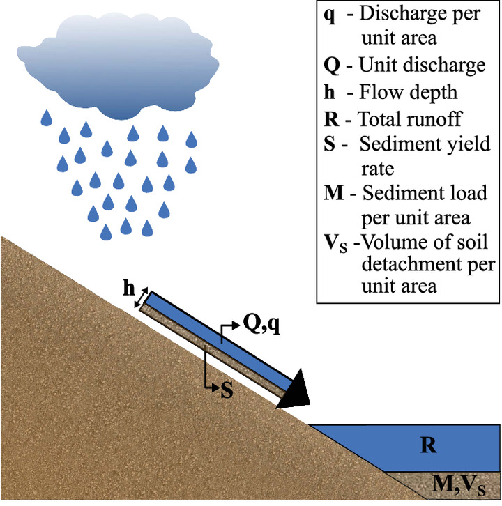
In this study, the Costa and Cavalcante (2021) constitutive model is used to describe the relationship between soil suction and unsaturated hydraulic conductivity of soil. This k-function is related to the Mein and Larson (1973) infiltration model by the suction at the wetting front. This model assumes soil homogeneity and the cumulative infiltration is obtained through an implicit equation in which the Napierian logarithm was approximated using Taylor series. The kinematic wave model, which is an approximate form of the water-continuity equation and the equation of motion, is used to describe the process of overland flow generation considering the transitional flow regime. For uniform rainfall conditions and considering the constant variations of the unit discharge with distance, these models help derive equations for the discharge per unit area (q), unit discharge (Q), flow depth (h), and total runoff (R). Furthermore, the steady-state sediment continuity equation is used to predict interrill erosion as it incorporates splash erosion and runoff erosion. Since the infiltration capacity of the soil rapidly decreases at the start of the rainfall, the variation in the sediment concentration with time was neglected. The unit discharge and flow depth were used as input data to calculate the sediment yield rate (S), sediment load per unit area (M), and volume of soil detachment per unit area (V_s). The physical behavior of the governing equations for overland flow and sediment transport is illustrated in Fig. 1.

Fig. 1. Physical behavior of overland flow and sediment transport.

The primary parameters of the governing equations derived in this model are: the distance along the surface plane (z), time (t), rainfall intensity (p), rainfall duration (t_s), slope length (L), surface slope (J), saturated hydraulic conductivity of soil (k_s), saturated moisture content (θ_s), initial moisture content (θ_i), residual moisture content (θ_r), three fitting parameters (δ₁, δ₂, λ), Manning's roughness coefficient (n), void ratio (e), density of soil particles (ρ_s), density of water (ρ_w), gravitational acceleration (g), calibration constant of splash erosion (c_r), erodibility coefficient (K_e), and critical shear stress (τ_c).

The essence of our model lies in its innovative combination of various methodologies and equations, allowing it to capture the dynamics of overland flow and sediment transport with remarkable precision and efficiency. For instance, while models based on the FEM or finite-difference method (FDM) offer significant details, they often require substantial computational resources, which our model circumvents with its analytical core. Conversely, traditional analytical models, while efficient, may lack the comprehensive representation of physical processes that our model provides by integrating elements from approaches based on computational fluid dynamics (CFD) or discrete-element method (DEM). This unique blend of methodologies, hence, allows our model to transcend the limitations inherent in each approach.

Coupling the k-Function to the Infiltration Model

The Mein–Larson model assumes that both the infiltration rate and cumulative infiltration equations are based on the suction at the wetting front (Mein and Farrell 1974), which is represented by

ψ_{f} = - \frac{1}{k_{s}} \int_{ψ_{i}}^{0} k (ψ) d ψ

(1)

where ψ_f, ψ_i, and ψ = suction at the wetting front, initial soil suction, and soil suction, respectively (M L⁻¹ T⁻²); and k_s and k = saturated hydraulic conductivity of the soil and unsaturated hydraulic conductivity of the soil, respectively (L T⁻¹).

The suction at the wetting front is a measure of the tension or negative pressure of the soil water. When water enters the soil, it fills the soil pores and creates a negative pressure that draws more water into the soil. This negative pressure is known as suction and is related to the soil water content. The suction at the wetting front is a critical parameter in the Mein–Larson model because it controls the rate at which water can infiltrate the soil.

k-Functions are commonly used in hydrology and soil science to describe the hydraulic conductivity of soil as a function of water content. The function is used to estimate the rate at which water can move through soil and is typically determined through laboratory measurements of the hydraulic conductivity of soil at different moisture contents. To determine the suction at the wetting front, a k-function needs to be defined. Cavalcante and Zornberg (2017) suggested using the following k-function for unimodal soils:

k (| ψ |) = k_{s} \exp (- δ | ψ |)

(2)

where δ = fitting hydraulic parameter (M⁻¹ L T²).

Durner (1992) proposed a method to estimate the soil–water retention curve for bimodal soils by using a linear superposition. The linear superposition model assumes that the water content in bimodal soils can be expressed as a combination of the water contents in the individual modes, weighted by their respective fractions in the soil. By superimposing the water retention curves for the individual modes, the model provides an estimate of the water retention curve for the bimodal soil. Costa and Cavalcante (2021) expanded Eq. (2) as follows to include bimodal soils by using a linear superposition of the unimodal curves, as outlined by Durner (1992):

k (| ψ |) = k_{s} [λ \exp (- δ_{1} | ψ |) + (1 - λ) \exp (- δ_{2} | ψ |)]

(3)

where λ = weight factor corresponding to the macroporous region; and δ₁ and δ₂ = fitting hydraulic parameters corresponding to the macroporous region and microporous region, respectively (L⁻¹).

Therefore, the suction at the wetting front for a unimodal soil can be obtained as follows by solving the integration that results from substituting Eq. (2) into Eq. (1):

ψ_{f} = \frac{1 - \exp (- δ ψ_{i})}{δ}

(4)

Similarly, the suction at the wetting front for a bimodal soil can be obtained as follows by solving the integration that results from substituting Eq. (3) into Eq. (1):

ψ_{f} = \frac{λ}{δ_{1}} [1 - \exp (- δ_{1} ψ_{i})] + \frac{1 - λ}{δ_{2}} [1 - \exp (- δ_{2} ψ_{i})]

(5)

Overland Flow Generation

The kinematic wave model is a simple mathematical model used to describe the movement of water over a surface during a rainfall event or flood. The proposed model assumes that water moves downstream as a wave, with its velocity determined by the slope of the surface and the roughness of the bed. The kinematic wave model is often used to approximate overland flow in hydrologic models and has been widely applied in a range of applications, such as flood forecasting, erosion control, and stormwater management. It assumes uniform flow, which means that the water depth and velocity are constant over the entire flow cross section. This makes it a relatively simple and computationally efficient model, but also limits its accuracy, especially when applied to nonuniform flow conditions.

Uniform rainfall conditions refer to a scenario where rainfall intensity is constant and evenly distributed over a given area and time. This means that the rainfall rate is the same at every point within the area being considered and does not vary significantly over time. Uniform rainfall conditions are often used as an assumption in hydrologic models to simplify calculations and to make them more manageable. However, rainfall is rarely uniformly distributed, and variations in rainfall intensity and spatial distribution can have a significant impact on hydrologic processes and water flow.

It's important to note that the physicomathematical model proposed in this study was developed based on uniform rainfall conditions, with overland flow generation approximated using the kinematic wave model, as explained by Henderson and Wooding (1964), as follows:

\frac{\partial Q (z, t)}{\partial z} + \frac{\partial h (z, t)}{\partial t} = r_{e} (t)

(6)

where Q = unit discharge (L² T⁻¹); z = distance along the surface plane (L); h = flow depth (L); t = time (T); and r_e = excess rainfall intensity (L T⁻¹).

Despite its limitations, the kinematic wave model has been widely used in hydrology and water resources engineering for over half a century and is still an important tool for many practical applications. Many more advanced hydrologic and hydraulic models, such as the Saint-Venant equations or the Navier–Stokes equations, are more complex and computationally demanding, hence the kinematic wave model can be a useful alternative when rapid estimates are required.

The unit discharge can be determined by expressing it as a function of the flow depth. During the transitional flow regime, this equation can be approximated as follows, as outlined by Horton (1937), Giráldez and Woolhiser (1996), Agnese et al. (2001), Singh (2002), Baiamonte and Agnese (2010), and Tao et al. (2018):

Q (z, t) = \frac{J^{1 / 2}}{n} h (z, t)^{2}

(7)

where J = surface slope (L L⁻¹); and n = Manning's roughness coefficient (T L^−1/3).

The transitional flow regime refers to a state between two flow regimes, typically laminar and turbulent flow. This occurs when the flow conditions, such as the velocity or Reynolds number, are such that the flow is not purely laminar or purely turbulent, but a combination of both. During the transitional flow regime, the flow is often characterized by fluctuations in velocity and pressure, and the formation of vortices and eddies. It is often difficult to model and predict, as the flow behavior can be highly sensitive to minor changes in the flow conditions or the boundary conditions. This contrasts with laminar flow, which is more predictable and easier to model, and turbulent flow, which can be modeled using statistical techniques, such as the Reynolds-averaged Navier–Stokes equations.

It is pertinent to mention that the excess rainfall intensity is not assumed to be constant in this physicomathematical model because the infiltration rate is also not constant. Mein and Larson (1973) provided a definition of the infiltration rate both before and after the ponding time, as follows:

f (t) = {\begin{matrix} p; & t < t_{p} \\ k_{s} [1 + \frac{ψ_{f} (θ_{s} - θ_{i})}{F (t)}]; & t \geq t_{p} \end{matrix}

(8)

where f = infiltration rate (L T⁻¹); p = rainfall intensity (L T⁻¹); t_p = ponding time (T); θ_s and θ_i = saturated moisture content and initial moisture content, respectively (L³ L⁻³); and F = cumulative infiltration (L).

The infiltration rate refers to the velocity at which water is able to penetrate or soak into the soil surface. Ponding time, conversely, refers to the length of time that water stands on the surface of the ground before it is able to infiltrate into the soil. This can happen when the infiltration rate is slower than the rate at which water is falling or accumulating on the surface, or when the soil is already saturated with water.

Cumulative infiltration is the total amount of water that has infiltrated into the soil from the start of the rainfall event up to a particular point in time. Mein and Larson (1973) provided a definition of the cumulative infiltration as an implicit equation, meaning it can be estimated through an iterative process to determine the infiltration rate, as follows:

\begin{aligned} F (t) - & \frac{k_{s} ψ_{f} (θ_{s} - θ_{i})}{p - k_{s}} \\ - ψ_{f} (θ_{s} - θ_{i}) \ln [\frac{ψ_{f} (θ_{s} - θ_{i}) + F (t)}{ψ_{f} (θ_{s} - θ_{i}) + ((k_{s} ψ_{f} (θ_{s} - θ_{i})) / (p - k_{s}))}] \\ (9) & = k_{s} [t - \frac{k_{s} ψ_{f} (θ_{s} - θ_{i})}{p (p - k_{s})}] \end{aligned}

(9)

The excess rainfall intensity is then calculated as the difference between the rainfall intensity and the infiltration rate. A detailed explanation of the development of the equations for discharge per unit area, unit discharge, flow depth, and total runoff is presented in Appendix I.

Sediment Transport

This physicomathematical model uses a simplified version of the steady-state sediment continuity equation to describe sediment transport during a rainfall event. Since the sediment concentration tends to stabilize as the infiltration capacity of the soil rapidly declines at the start of the rainfall (Foster and Meyer 1972; Beasley et al. 1980; Yu 2003), the partial derivative of time in the steady-state sediment continuity equation can be ignored (Nearing et al. 1989; Tao et al. 2018), given

\frac{\partial [s (z, t) Q (z, t)]}{\partial z} = \frac{c_{r} p^{2}}{ρ_{d}} + K_{e} [ρ_{w} g J h (z, t) - τ_{c}]

(10)

where s = sediment concentration (M L⁻³); ρ_d and ρ_w = dry density of soil and density of water, respectively (M L⁻³); c_r = calibration constant of splash erosion (M² T L⁻⁷); K_e = erodibility coefficient (T L⁻¹); g = gravitational acceleration (L T⁻²); and τ_c = critical shear stress (M L⁻¹ T⁻²).

The sediment yield rate is the amount of sediment that is transported by water per unit area. It is calculated by multiplying the sediment concentration (the amount of sediment in the water) by the discharge (the amount of water flowing per unit time) per unit area, as follows:

S (z, t) = s (z, t) q (t)

(11)

where S = sediment yield rate (M L⁻² T⁻¹); and q = discharge per unit area (L T⁻¹).

The sediment yield rate is an important parameter in the study of soil erosion and sediment transport, as it provides information on the amount of sediment that is being carried by water from a particular area. It is influenced by a variety of factors, such as land use, soil type, slope, and precipitation patterns. Also, the scale effect on soil erosion is variable and dynamic for different erosion types, rainfall intensities, and soil characteristics, as discussed by Wu et al. (2021).

The development of the equations for sediment yield rate, sediment load per unit area, and volume of soil detachment per unit area is detailed in Appendix II.

Experimental Test

The model was calibrated using Brazilian Latosol soil collected from the Itumbiara Plant's water reservoir. The Itumbiara Plant is located on the Paranaíba River between the cities of Itumbiara and Araporã in Brazil (18°24′27″ S, 49°05′59″ W). This hydroelectric power plant has an installed capacity of 2.082 MW, and its water reservoir covers 798 km² of flooded area, according to Eletrobras Furnas (2019). The soil in this area is predominantly lateritic with a bimodal soil–water retention curve (Merabet Júnior 2022). The soil's saturated hydraulic conductivity is 0.024 cm/min, and the density of the soil particles is 2.62 g/cm³.

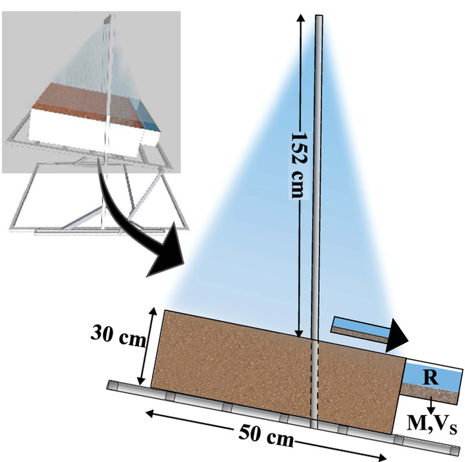
Merabet Júnior (2022) used a rainfall simulator built by Melo (2020) with 50 cm slope length to collect experimental data on discharge per unit area, total runoff, sediment yield rate, and sediment load per unit area. A scheme of the rainfall simulator used is presented in Fig. 2. The experiments were conducted on compacted soil samples from the right bank of the Itumbiara Plant's water reservoir. The soil characteristics are reported in Table 1. Six tests were conducted for 60 min, with variations in the rainfall intensity, surface slope, initial moisture content, and void ratio.

Fig. 2. Geometry of the rainfall simulator used in the experiments.

Table 1. Rainfall simulator tests performed by Merabet Júnior (2022)

Test	Rainfall intensity (mm/h)	Surface slope (°)	Initial moisture content (%)	Void ratio
1	248	5	32.4	1.05
2	248	5	33.1	0.97
3	248	5	20.7	1.08
4	233	15	33.5	1.00
5	233	15	35.3	1.02
6	233	15	20.2	1.12

Source: Data from Merabet Júnior (2022).

By measuring the effects of the rainfall intensity, surface slope, initial moisture content, and void ratio on sediment transport, researchers can better understand the complex interplay of factors that contribute to soil erosion and sediment transport. This information can be used to develop strategies to minimize soil erosion and protect downstream water quality.

Higher rainfall intensities can increase the potential for erosion and sediment transport, especially on bare or poorly vegetated soils. Surface slope also plays a role in erosion and sediment transport, as steeper slopes can increase the velocity of runoff and the potential for sediment to be transported downhill. Initial moisture content and void ratio are both related to the soil porosity and can influence how water moves through the soil. Soils presaturated with water may exhibit a reduced capacity to absorb additional rainfall, thereby elevating the likelihood of increased runoff and erosion. Conversely, soils with a lower initial moisture content may be less vulnerable to erosion during rainfall events, as they have a higher capacity to absorb and retain water. Void ratio, which is the ratio of the volume of voids in the soil to the volume of solid particles, can influence the ability of the soil to absorb and retain water.

Table 1 indicates that the soil samples used in the study had different surface slope conditions and initial moisture contents for each of the tests conducted. These different slope conditions were adopted for a better comprehension of the effects of the surface slope on sediment transport under different rainfall conditions, while the variation in initial moisture content aimed to understand the impact of soil saturation levels on sediment transport.

To couple the k-function to the infiltration model, the parameters λ, δ₁, and δ₂ needed to be defined. Experimental data from the soil–water retention curve (SWRC), which was obtained by Merabet Júnior (2022), were used to calibrate these parameters with a nonlinear fit applied to the Costa and Cavalcante (2021) SWRC model, as follows:

\begin{aligned} θ (| ψ |) = θ_{r} + (θ_{s} - θ_{r}) [λ \exp (- δ_{1} | ψ |) + (1 - λ) \exp (- δ_{2} | ψ |)] \end{aligned}

(12)

where θ and θ_r = moisture content and residual moisture content, respectively (L³ L⁻³).

To apply the physicomathematical model, several other necessary parameters, such as Manning's roughness coefficient, erodibility coefficient, calibration constant of splash erosion, and critical shear stress, were defined based on experimental data of the total runoff and sediment load per unit area. Manning's roughness coefficient was set at 0.025 s/m^1/3, which is a value typically associated with straight and uniform channels in poor conditions, as reported by Neves (1960). After calibration using a nonlinear model fit based on experimental data of the total runoff and sediment load per unit area, the calibration constant of splash erosion and critical shear stress were both set to zero. The erodibility coefficient was set at 0.005 g/cm²/min/Pa, which is classified as medium erodibility soil according to Bastos (1999).

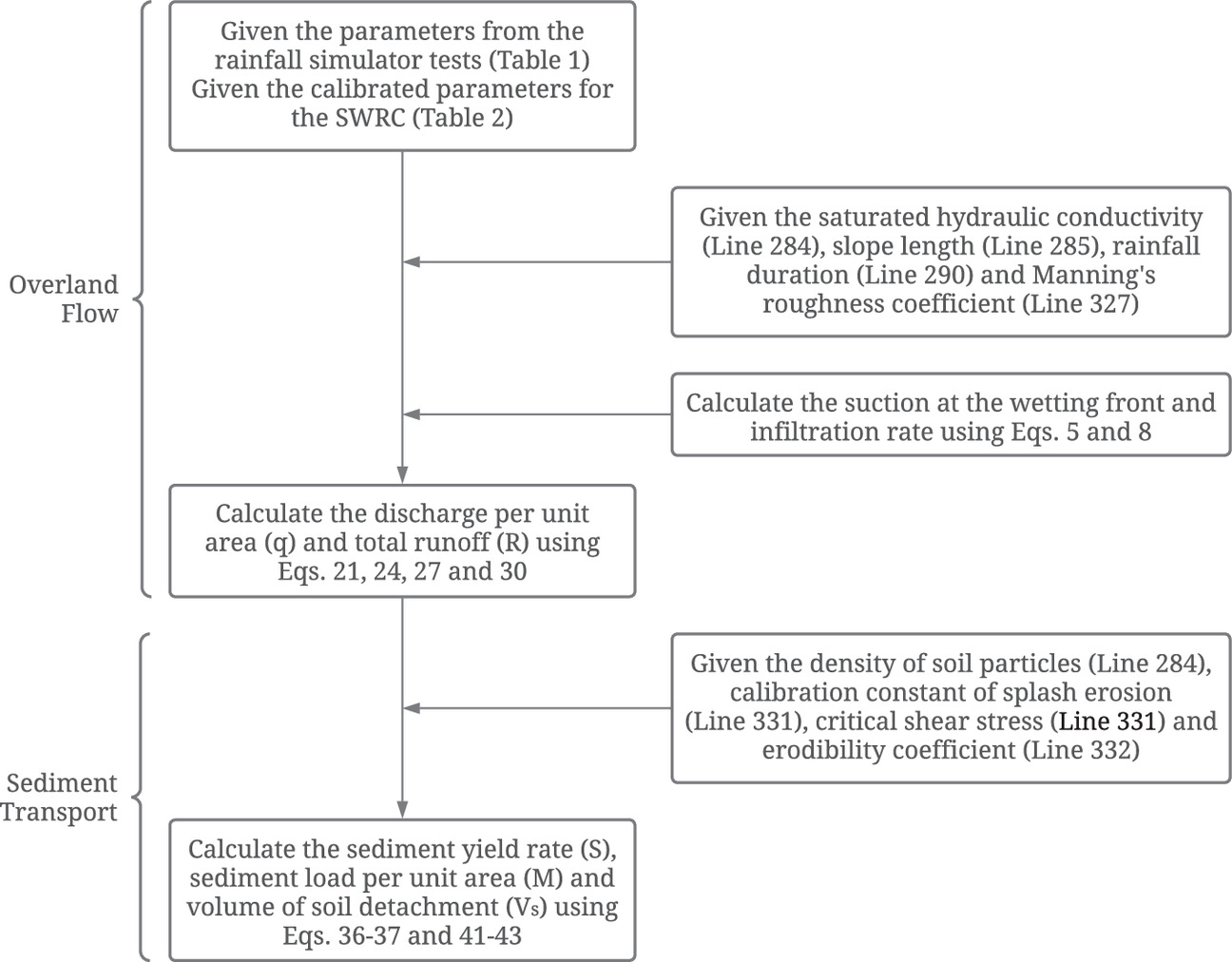
The governing equations of the physicomathematical model were calculated using the flow chart presented in Fig. 3, which sums up the derivation logic systematically. All equations and graphics were implemented using Wolfram Mathematica 12.3. No numerical tools were used in this study because the systems of equations were solved analytically. The correspondence between the experimental data and the results obtained from the model was evaluated using the coefficient of determination.

Fig. 3. Flow chart for calculating overland flow and sediment transport equations.

Results and Discussion

Soil–Water Retention Curve

The Costa and Cavalcante (2021) SWRC model was mathematically fine-tuned using a nonlinear model fit with Merabet Júnior (2022) experimental data on the SWRC. The resulting parameters are provided in Table 2.

Table 2. Costa and Cavalcante SWRC model calibrated parameters

θ_s (%)	θ_r (%)	δ₁ (kPa⁻¹)	δ₂ (kPa⁻¹)	λ (%)
45.15	1.28	0.065656	5.25 × 10⁻⁵	47.85

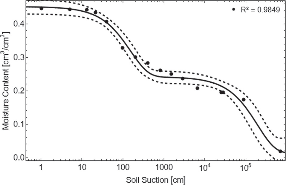
When these parameters were applied to Eq. (12), the model was found to fit the experimental data very well, with a coefficient of determination of 0.98. As shown in Fig. 4, 14 out of the 16 experimental points were within the 95% mean prediction confidence bands.

Fig. 4. Costa and Cavalcante SWRC model adherence to the experimental data.

Overland Flow Generation

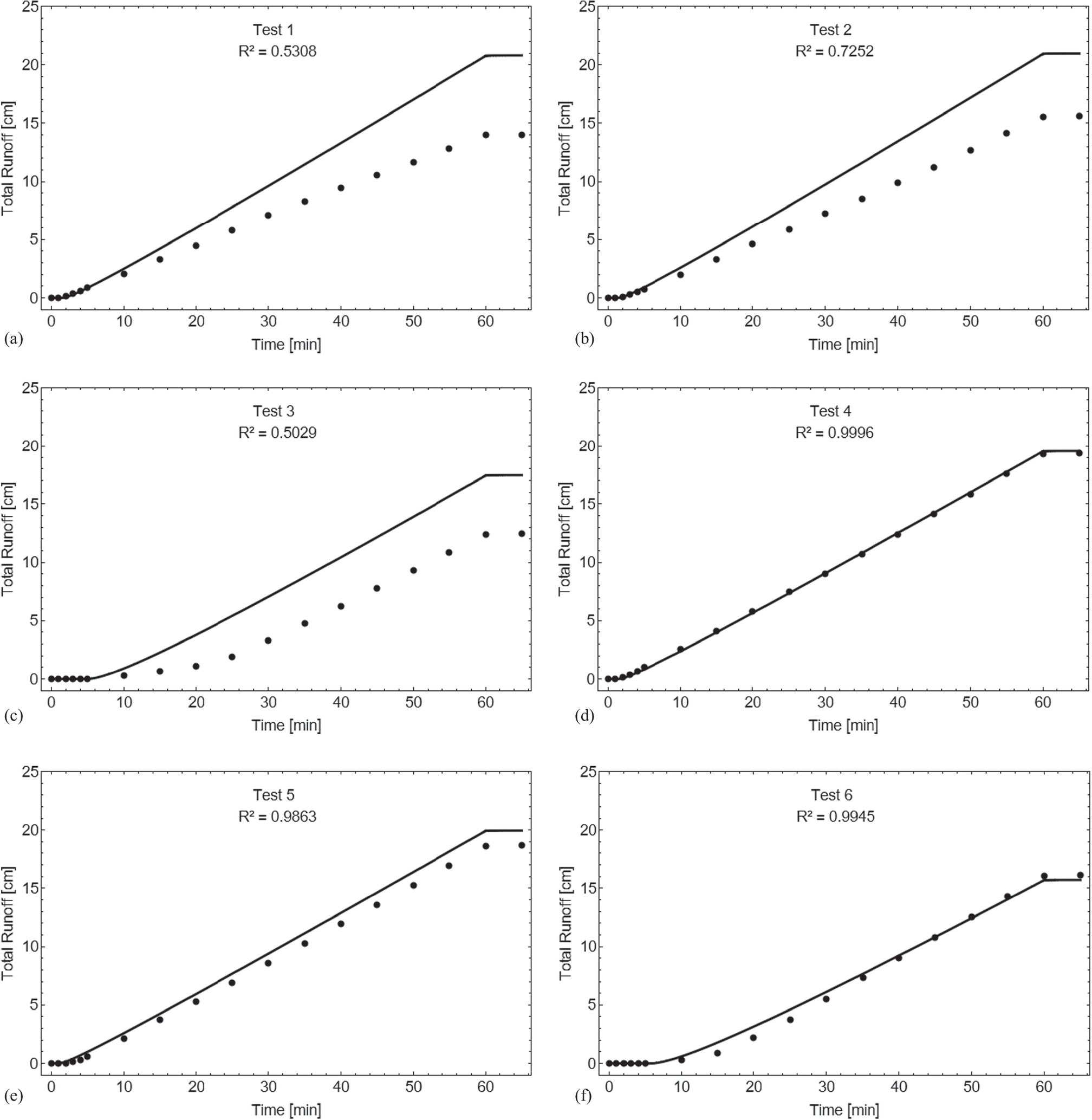
From Figs. 5 and 6, it can be seen that the experimental data on discharge per unit area initially increases and then stabilizes in a steady state, while the total runoff increases linearly until the end of the rainfall event.

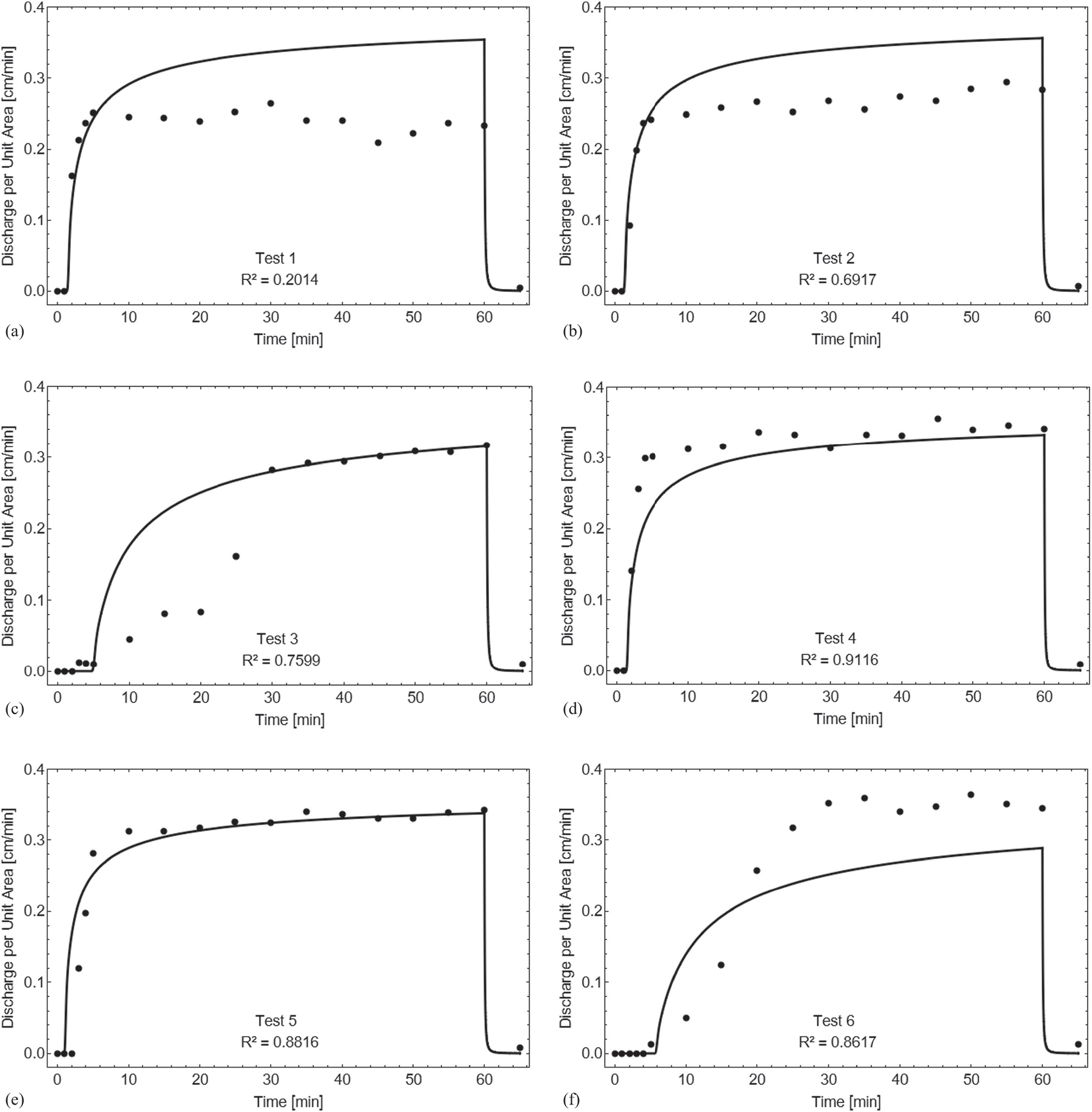
Fig. 5. Discharge per unit area model compared with experimental data for (a) Test 1; (b) Test 2; (c) Test 3; (d) Test 4; (e) Test 5; and (f) Test 6.

Fig. 6. Total runoff model compared with experimental data for (a) Test 1; (b) Test 2; (c) Test 3; (d) Test 4; (e) Test 5; and (f) Test 6.

When comparing surface slopes, the tests with a 15° slope show a higher discharge per unit area and total runoff after 60 min than the tests with a 5° slope. This is expected because as the slope increases, the infiltration rate decreases, as noted by Blight (1997). However, the discharge per unit area model, which uses Eq. (21), is not sensitive to changes in the surface slope because the parameter α is embedded within a hyperbolic tangent function. In comparison, the tests with a 15° slope show better agreement with the experimental data (R² values between 0.86 and 0.92) than the tests with a 5° slope (R² values between 0.20 and 0.76). Similar results have been found by Abrantes et al. (2021), whose numerical model only properly simulated runoff observed with the higher slope of 10%, while poor agreement with the experimental data was observed with the lower slope of 1%. At a steeper slope, the gravitational component is more significant, making the flow more deterministic and easier to capture with the model. For further investigation into this aspect, more tests need to be performed under different circumstances of rainfall intensity, surface slope, and initial moisture content.

The soil samples with lower initial moisture content took longer to reach a steady state of discharge per unit area, resulting in a lower total runoff by the end of the rainfall event. The discharge per unit area model is better at representing the rise in discharge when the initial moisture content is higher, but there was no correlation between higher initial moisture content and a higher coefficient of determination. Surprisingly, the test with the lowest initial moisture content among the tests with a 5° slope had the highest R² (0.76) as this test did not overestimate the discharge per unit area during steady state.

Comparing the discharge per unit area model with the total runoff model, the latter had a higher mean coefficient of determination (0.72 versus 0.79). This is because Eq. (24) has the parameter α outside of the hyperbolic tangent function, making the total runoff model a little more sensitive to variation in the surface slope. However, this effect was not evident in the slope interval studied. The tests with a 15° slope had almost perfect correspondence with the experimental data (R² > 0.98), and like the discharge per unit area model, there was no correlation between higher initial moisture content and a higher coefficient of determination in the total runoff model.

Sediment Transport

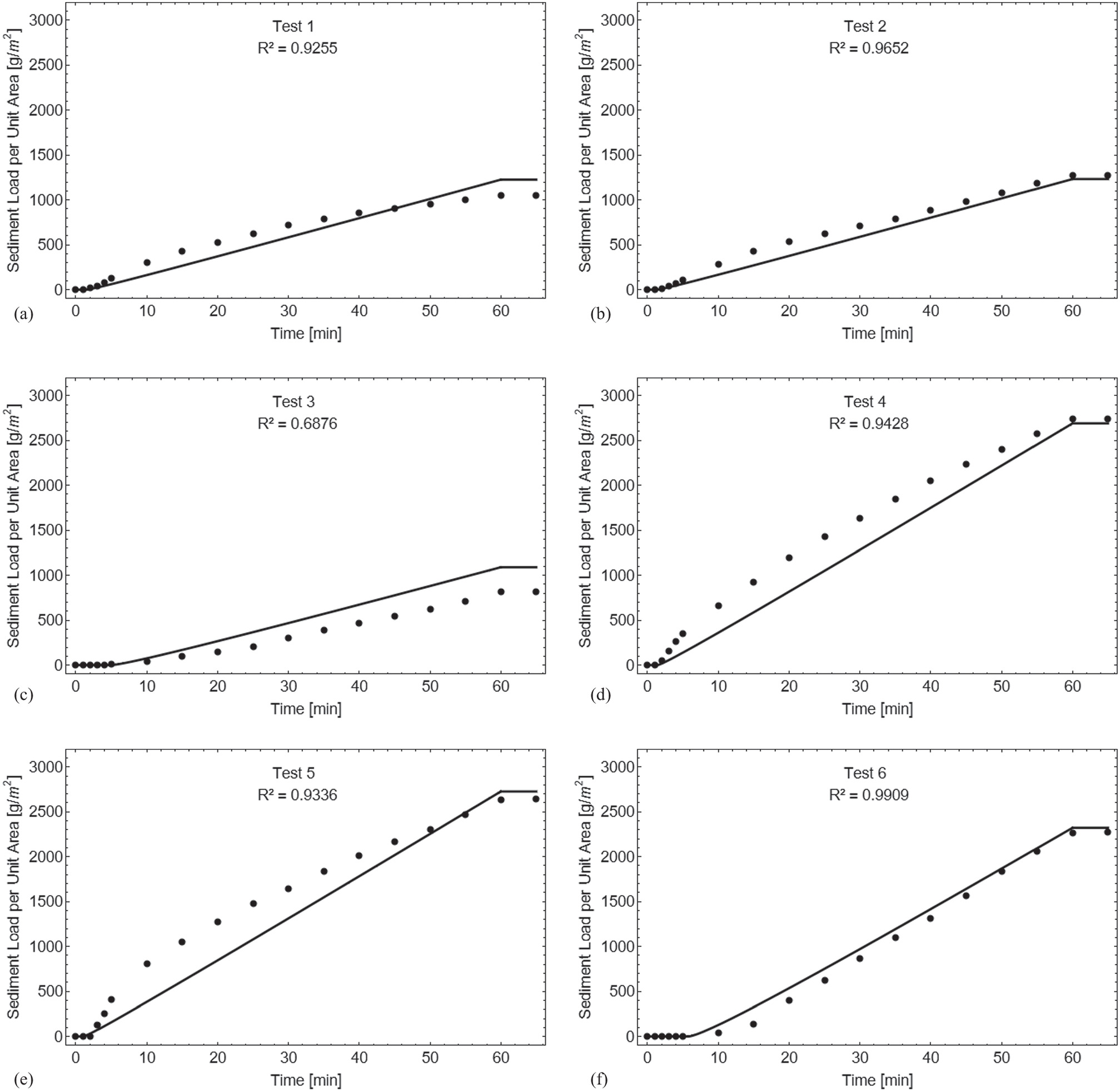
As presented in Fig. 7, the experimental data on sediment yield rate rises followed by a threshold, similar to the pattern observed in the discharge per unit area. However, there is a peak in the sediment yield rate around 5 min after the start of rainfall, which is due to raindrop impact detaching the soil particles. After this peak, the sediment yield rate decreases as flow shear becomes the dominant detachment mechanism. The tests with lower initial moisture content reach a steady state without this peak in the sediment yield rate in the initial minutes of rainfall. Similarly, Fig. 8 shows that the experimental data on sediment load per unit area is analogous to the total runoff, but with a change in the slope as a result of a change in the dominant detachment mechanism: a higher slope due to raindrop impact and a lower slope due to flow shear.

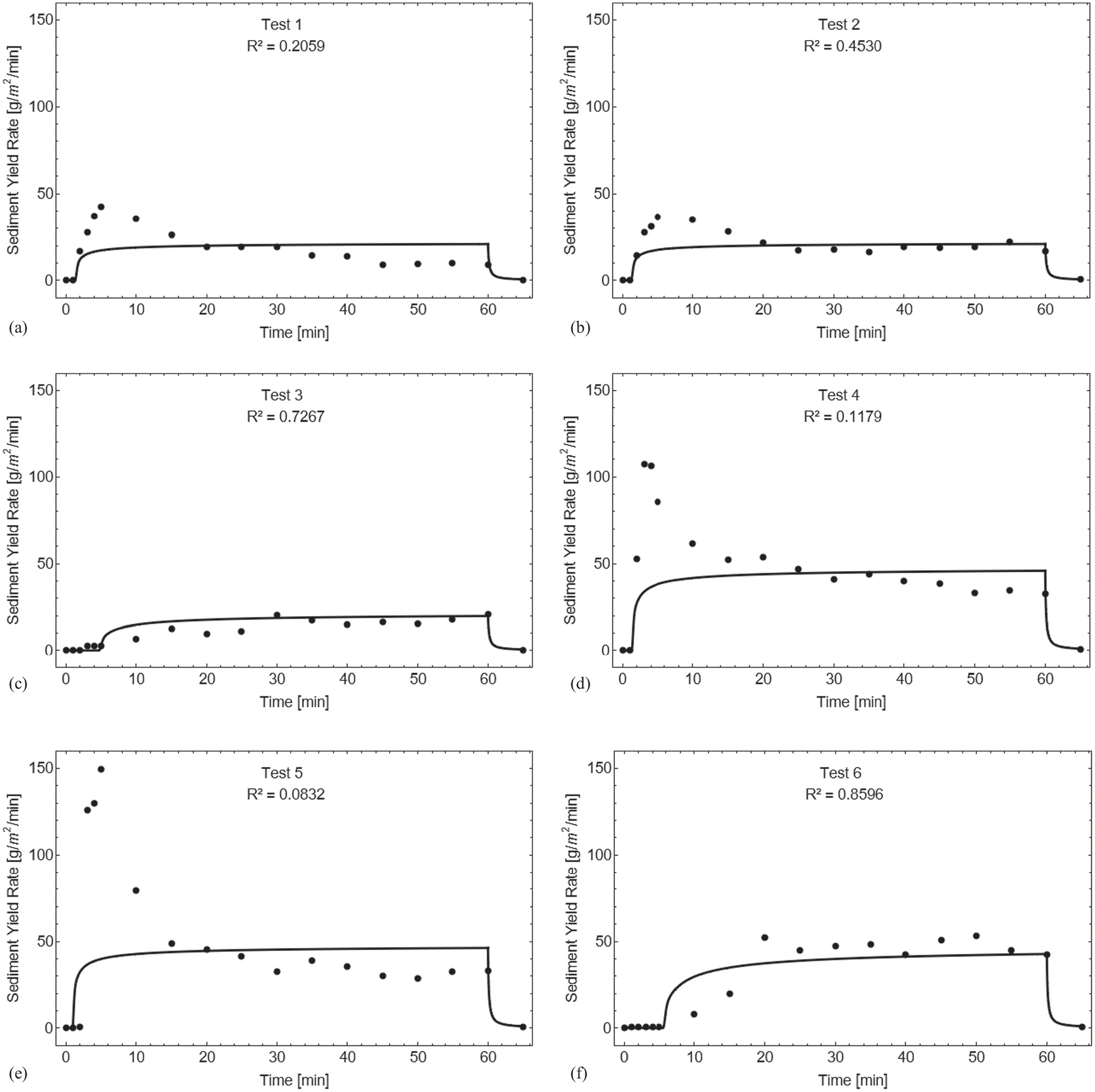
Fig. 7. Sediment yield rate model compared with experimental data for (a) Test 1; (b) Test 2; (c) Test 3; (d) Test 4; (e) Test 5; and (f) Test 6.

Fig. 8. Sediment load per unit area model compared with experimental data for (a) Test 1; (b) Test 2; (c) Test 3; (d) Test 4; (e) Test 5; and (f) Test 6.

As expected, the tests with a 15° slope produced higher sediment yield rates and sediment loads per unit area after 60 min compared with the tests with a 5° slope. This was also observed with the discharge per unit area and total runoff. When higher initial moisture content was used, the peak of sediment yield rate was even greater in the tests with a 15° slope, indicating that increasing the slope has a positive effect on detachment by raindrop impact, as observed by Zhang et al. (2019). However, there was no clear correlation between surface slope and better correspondence with the experimental data, as the coefficient of determination had a high variance for both 5° (0.20 < R² < 0.73) and 15° (0.08 < R² < 0.86) slopes.

The sediment yield rate model has a limitation of not accounting for the initial peak in the sediment yield that occurs within the first few minutes of the rainfall. This is because the parcel of splash erosion in Eq. (10) is assumed to be constant. To address this limitation, the parameter c_r should vary with time, so that after a certain period, the parcel of splash erosion would become zero and sediment transport would be described only by rill erosion. The tests with lower initial moisture content showed better agreement with the experimental data, with R² values ranging from 0.76 to 0.86, despite the expectation of reaching a steady state. Therefore, the peak in the sediment yield rate observed in the initial minutes of the rainfall may be related to the critical shear stress, which depends on the antecedent soil moisture, as suggested by Li et al. (2022), and its accountability should be further investigated to improve the sediment yield rate model.

The sediment load per unit area model displays a linear increase over time, which is expected to capture the average of the detachment mechanisms required to match the sediment load per unit area of the experimental data at the conclusion of the rainfall event. Consistent with the sediment yield rate model, the tests conducted on a 15° slope exhibited higher sediment load per unit area values at the end of the 60-min rainfall event when compared with the tests carried out on a 5° slope.

The model for sediment concentration had the highest mean coefficient of determination (0.91) compared with the other four models evaluated. The data showed strong agreement with the experimental results, with five out of six tests having a coefficient of determination greater than 0.92. There was no clear correlation between the initial moisture content and the coefficient of determination. Test 3, which had a lower initial moisture content and a 5° slope, had the lowest R² value (0.69), while Test 6, which also had a lower initial moisture content but a 15° slope, had the highest R² value (0.99).

Parametric Analysis

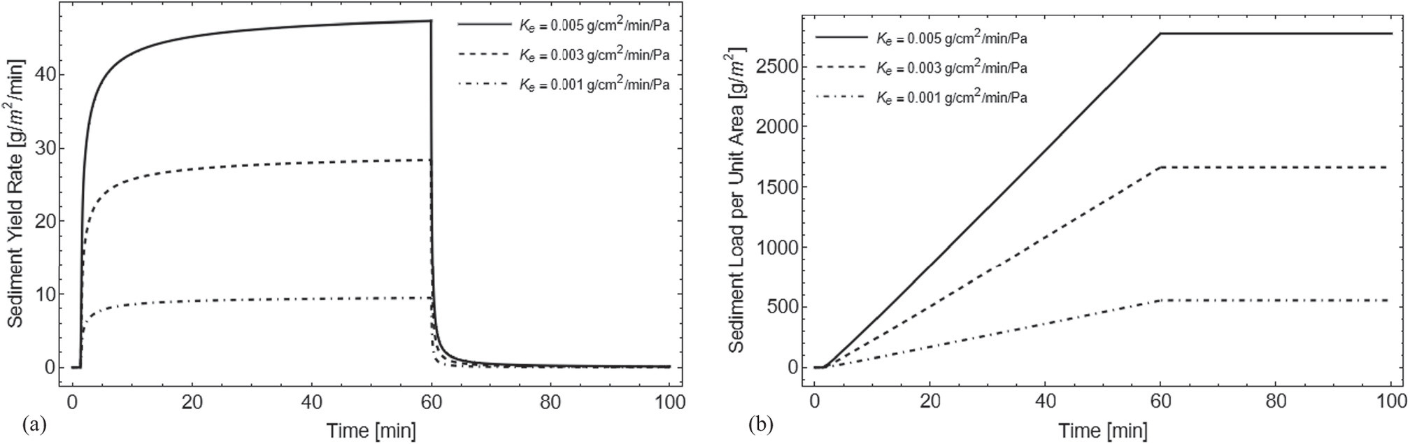
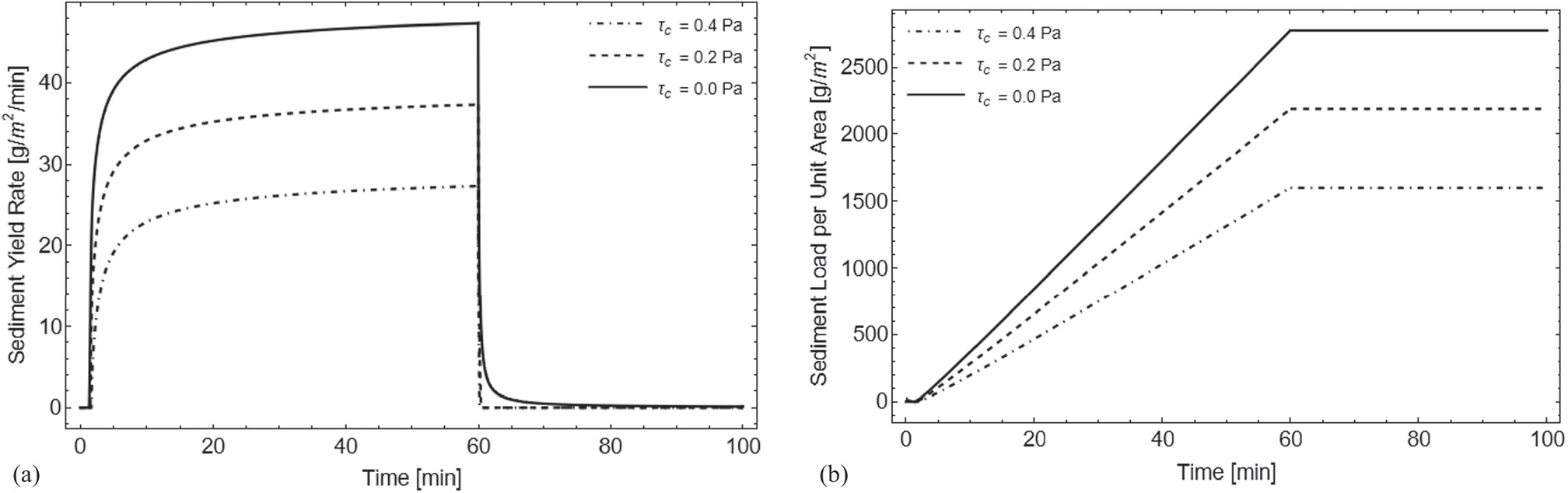
To investigate the effects of calibration constants on the sediment yield rate and sediment load per unit area equations, the authors conducted parametric analysis using three values for each constant: c_r (0.0, 0.005, and 0.010 g² min/cm⁷), K_e (0.001, 0.003, and 0.005 g/cm²/min/Pa), and τ_c (0.0, 0.2, and 0.4 Pa).

It could be seen in Figs. 9 and 10 that the sediment yield rate model is extended during steady state by increasing the calibration constant of splash erosion and erodibility coefficient, resulting in an increased slope of the sediment load per unit area model during its rise. Conversely, increasing the critical shear stress has a negative effect on both models, as shown in Fig. 11. When the critical shear stress is exceeded, detachment by flow shear occurs (Kinnell 2021), leading to a reduction in the sediment yield rate model during steady state and a decrease in the slope of the sediment load per unit area model during its rise.

Fig. 9. Effect of the calibration constant of splash erosion on the (a) sediment yield rate; and (b) sediment load per unit area.

Fig. 10. Effect of the erodibility coefficient on the (a) sediment yield rate; and (b) sediment load per unit area.

Fig. 11. Effect of the critical shear stress on the (a) sediment yield rate; and (b) sediment load per unit area.

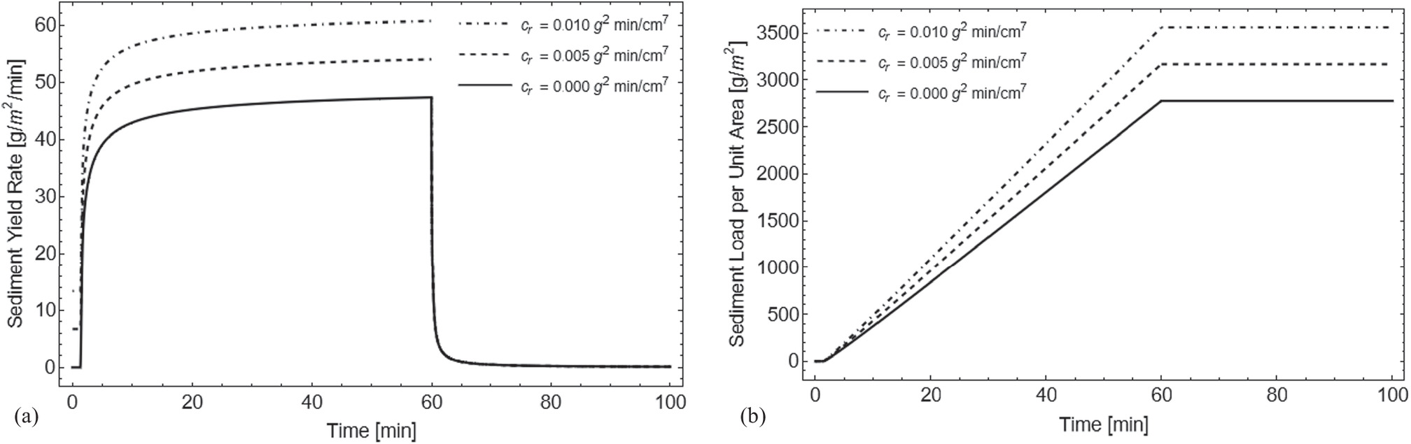
When the calibration constant of splash erosion is nonzero, there is a noticeable change in the sediment yield rate model as it transitions from the rising stage to the recession stage. Specifically, during the rising stage, the sediment yield rate model shifts upwards and no longer matches the sediment yield rate model during the recession stage at 60 min. This is because the equation does not account for the calibration constant of splash erosion during the recession stage. However, assuming that the calibration constant of splash erosion is zero is not accurate, as it assumes that rainfall erosion is driven solely by flow. To address this issue, the parameter c_r should vary with time and eventually become zero before the recession stage.

Conclusions

In this study, a one-dimensional physicomathematical model was developed to simulate overland flow and sediment transport in high-intensity rainfall simulator tests. The model includes equations for discharge per unit area, total runoff, sediment yield rate, and sediment load per unit area, and was validated using experimental data. The Mein–Larson infiltration model was employed to estimate the amount of rainfall converted into overland flow. The kinematic wave model effectively described overland flow during transitional flow, and the steady-state sediment continuity equation successfully described sediment transport. The soil–water retention curve was estimated using the Costa and Cavalcante SWRC model, which is designed for bimodal soils.

The physicomathematical model satisfactorily represented the experimental data, demonstrating a threshold in the discharge per unit area and sediment yield rate models, and a linear increase in the total runoff and sediment load per unit area models. The model could not fully account for the minimal variation in the discharge per unit area with slope, which would be consistent with the experimental data. The models for discharge per unit area and total runoff were more accurate for tests with a 15° slope than those with a 5° slope.

The sediment yield rate model captured the threshold when flow shear became the dominant detachment mechanism, but it did not account for the peak in the initial minutes of rainfall owing to detachment by raindrop impact. This can be addressed by making the parameter c_r a function of time that becomes null when the overland flow begins. When the parameter c_r is zero, the sediment yield rate model represents better the tests with lower initial moisture content. The sediment load per unit area model had a high coefficient of determination (0.91), indicating strong agreement with the experimental data.

It was demonstrated by parametric analysis that increasing the calibration constant of splash erosion and erodibility coefficient increases the slope of the sediment load per unit area model during its rise. Conversely, increasing the critical shear stress decreases the slope of the sediment load per unit area model during its rise. The authors also found that when the calibration constant of splash erosion was nonzero, the sediment yield rate model shifted upwards during the rising stage and no longer matched the model during the recession stage at the time of the rainfall.

Overall, the physicomathematical model proved to be a useful tool in predicting the total runoff and sediment load per unit area in high-intensity rainfall simulator tests and can help inform management practices for soil conservation and erosion control.

Appendix I. Overland Flow Generation

The expression for the unit discharge can be derived by assuming a constant variation of the unit discharge with distance, as follows:

Q (z, t) = q (t) z

(13)

Eq. (7) can be equated to Eq. (13) as follows:

\frac{J^{1 / 2}}{n} h (z, t)^{2} = q (t) z

(14)

To simplify the equations, the parameter α is defined as follows:

α = \frac{J^{1 / 2}}{n}

(15)

After substituting Eq. (15) into Eq. (14), the flow depth can be isolated as follows:

h (z, t) = {(\frac{z}{α} q (t))}^{1 / 2}

(16)

One can obtain the derivative with respect to time of Eq. (16) as follows:

\frac{\partial h (z, t)}{\partial t} = \frac{1}{2} {(\frac{z}{α})}^{1 / 2} q {(t)}^{- 1 / 2} \frac{d q (t)}{d t}

(17)

The kinematic wave model can be expressed by substituting Eqs. (13) and (17) into Eq. (6), as follows:

q (t) + \frac{1}{2} {(\frac{z}{α})}^{1 / 2} q {(t)}^{- 1 / 2} \frac{d q (t)}{d t} = r_{e} (t)

(18)

To integrate Eq. (18), both sides were taken into consideration with respect to distance from 0 to L. Then, the instantaneous time change dt was isolated to obtain the following:

d t = \frac{1}{3} {(\frac{L}{α})}^{1 / 2} \frac{q {(t)}^{- 1 / 2}}{r_{e} (t) - q (t)} d q (t)

(19)

where L = slope length (L).

During the Rainfall Event

To integrate Eq. (19), both sides were taken into consideration with respect to time starting from the ponding time and ending at a time just prior to the conclusion of the rainfall event:

t - t_{p} = \frac{1}{3} {(\frac{L}{α})}^{1 / 2} \int_{q (t_{p})}^{q (t)} \frac{q {(t)}^{- 1 / 2}}{r_{e} (t) - q (t)} d q (t)

(20)

The discharge per unit area in the rising stage is obtained by solving Eq. (20), as follows:

q (t) = \tanh^{2} (\frac{3}{2} \sqrt{\frac{α r_{e} (t)}{L}} (t - t_{p})) r_{e} (t)

(21)

The unit discharge in the rising stage is obtained by substituting Eq. (21) into Eq. (13), as follows:

Q (z, t) = \tanh^{2} (\frac{3}{2} \sqrt{\frac{α r_{e} (t)}{L}} (t - t_{p})) r_{e} (t) z

(22)

The flow depth in the rising stage is reformulated by substituting Eq. (21) into Eq. (16), as follows:

h (z, t) = \sqrt{\frac{r_{e} (t) z}{α}} \tanh (\frac{3}{2} \sqrt{\frac{α r_{e} (t)}{L}} (t - t_{p}))

(23)

The total runoff in the rising stage is obtained by integrating Eq. (21) with respect to time from the ponding time to a time prior to the end of the rainfall event, as follows:

R (t) = r_{e} (t) (t - t_{p}) - \frac{2}{3} \sqrt{\frac{r_{e} (t) L}{α}} \tanh (\frac{3}{2} (t - t_{p}) \sqrt{\frac{α r_{e} (t)}{L}})

(24)

where R = total runoff (L).

After the Rainfall Event

When rainfall stops, the excess rainfall intensity becomes zero, and Eq. (19) simplifies to

d t = - \frac{1}{3} {(\frac{L}{α})}^{1 / 2} q {(t)}^{- 3 / 2} d q (t)

(25)

Integrating both sides of Eq. (25) with respect to time from the rainfall duration to a time t, we obtain the following:

(t - t_{s}) = - \frac{1}{3} {(\frac{L}{α})}^{1 / 2} \int_{q (t_{s})}^{q_{r} (t)} q {(t)}^{- 3 / 2} d q (t)

(26)

where t_s = rainfall duration (T).

The discharge per unit area in the recession stage is obtained by solving Eq. (26), as follows:

q_{r} (t) = q (t_{s}) {(1 + \frac{3}{2} (t - t_{s}) \sqrt{\frac{α q (t_{s})}{L}})}^{- 2}

(27)

To obtain the unit discharge in the recession stage, one can substitute Eq. (27) into Eq. (13), as follows:

Q_{r} (z, t) = q (t_{s}) {(1 + \frac{3}{2} (t - t_{s}) \sqrt{\frac{α q (t_{s})}{L}})}^{- 2} z

(28)

The flow depth in the recession stage is reformulated substituting Eq. (27) into Eq. (16), as follows:

h_{r} (z, t) = \sqrt{\frac{q (t_{s}) z}{α}} {(1 + \frac{3}{2} (t - t_{s}) \sqrt{\frac{α q (t_{s})}{L}})}^{- 1}

(29)

The total runoff in the recession stage is obtained by integrating Eq. (27) with respect to time from the end of the rainfall duration to the current time t, and then adding the result to the value of Eq. (24) at time t_s, as follows:

\begin{aligned} R_{r} (t) = r_{e} (t_{s}) (t_{s} - t_{p}) & - \frac{2}{3} \sqrt{\frac{r_{e} (t_{s}) L}{α}} \tanh (\frac{3}{2} (t_{s} - t_{p}) \sqrt{\frac{α r_{e} (t_{s})}{L}}) \\ + \frac{2}{3} \sqrt{\frac{q (t_{s}) L}{α}} - \frac{(4 / 9) \sqrt{((q (t_{s}) L) / α)}}{(2 / 3) + \sqrt{((α q (t_{s})) / L)} (t - t_{s})} \end{aligned}

(30)

Appendix II. Sediment Transport

For simplification reasons, the product of the sediment concentration and the unit discharge will be combined into a parameter Y, as follows:

Y (z, t) = s (z, t) Q (z, t)

(31)

During the Rainfall Event

After substituting Eq. (31) into Eq. (10), the steady-state sediment continuity equation is reformulated as follows:

\frac{\partial Y (z, t)}{\partial z} = \frac{c_{r} p^{2}}{ρ_{d}} + K_{e} [ρ_{w} g J h (z, t) - τ_{c}]

(32)

By substituting the expression in Eq. (23) into Eq. (32), we obtain the following:

\begin{aligned} \frac{\partial Y (z, t)}{\partial z} & = (\frac{c_{r} p^{2}}{ρ_{d}} - K_{e} τ_{c}) \\ + K_{e} ρ_{w} g J \sqrt{\frac{r_{e} (t)}{α}} z^{1 / 2} \tanh (\frac{3}{2} \sqrt{\frac{α r_{e} (t)}{L}} (t - t_{p})) \end{aligned}

(33)

Integrating both sides of Eq. (33) with respect to distance from 0 to z, we obtain the following:

\begin{aligned} Y (z, t) & = (\frac{c_{r} p^{2}}{ρ_{d}} - K_{e} τ_{c}) z \\ + \frac{2}{3} K_{e} ρ_{w} g J \sqrt{\frac{r_{e} (t)}{α}} z^{3 / 2} \tanh (\frac{3}{2} \sqrt{\frac{α r_{e} (t)}{L}} (t - t_{p})) \end{aligned}

(34)

Substituting Eqs. (11) and Eq. (13) into Eq. (31) defines the relationship between Y and the sediment yield rate, as follows:

Y (z, t) = S (z, t) z

(35)

To calculate the sediment yield rate during the rising stage, one can divide Eq. (34) by z, as follows:

S (z, t) = (\frac{c_{r} p^{2}}{ρ_{d}} - K_{e} τ_{c}) + \frac{2}{3} K_{e} ρ_{w} g J \sqrt{\frac{r_{e} (t) z}{α}} \tanh (\frac{3}{2} \sqrt{\frac{α r_{e} (t)}{L}} (t - t_{p}))

(36)

Since the distance along the surface plane is equivalent to the slope length, one can calculate the sediment load per unit area during the rising stage by integrating Eq. (36) with respect to time from the ponding time to a time prior to the end of the rainfall event, as follows:

\begin{aligned} M (t) & = (\frac{c_{r} p^{2}}{ρ_{d}} - K_{e} τ_{c}) (t - t_{p}) \\ + \frac{4}{9} K_{e} ρ_{w} g \sqrt{J} n L \ln {\cosh [\frac{3}{2} \sqrt{\frac{α r_{e} (t)}{L}} (t - t_{p})]} \end{aligned}

(37)

where M = sediment load per unit area (M L⁻²).

After the Rainfall Event

After rainfall ceases, the rainfall intensity is zero, and Eq. (32) simplifies to

\frac{\partial Y_{r} (z, t)}{\partial z} = K_{e} [ρ_{w} g J h_{r} (z, t) - τ_{c}]

(38)

By substituting Eq. (29) into Eq. (38):

\frac{\partial Y_{r} (z, t)}{\partial z} = K_{e} [ρ_{w} g J \sqrt{\frac{q (t_{s})}{α}} {(1 + \frac{3}{2} (t - t_{s}) \sqrt{\frac{α q (t_{s})}{L}})}^{- 1} z^{1 / 2} - τ_{c}]

(39)

By integrating both sides of Eq. (39) with respect to distance from 0 to z, we obtain

\begin{aligned} Y_{r} (z, t) = \frac{2}{3} K_{e} ρ_{w} g J \sqrt{\frac{q (t_{s})}{α}} {(1 + \frac{3}{2} (t - t_{s}) \sqrt{\frac{α q (t_{s})}{L}})}^{- 1} z^{3 / 2} - K_{e} τ_{c} z \end{aligned}

(40)

To calculate the sediment yield rate during the recession stage, one can divide Eq. (40) by z, as follows:

\begin{aligned} S_{r} (z, t) = \frac{2}{3} K_{e} ρ_{w} g J \sqrt{\frac{q (t_{s})}{α}} {(1 + \frac{3}{2} (t - t_{s}) \sqrt{\frac{α q (t_{s})}{L}})}^{- 1} z^{1 / 2} - K_{e} τ_{c} \end{aligned}

(41)

Since the distance along the surface plane is equivalent to the slope length, one can calculate the sediment load per unit area during the recession stage by integrating Eq. (41) with respect to time from the end of the rainfall duration to the current time t, and then adding the result to Eq. (37) at time t_s as follows:

\begin{aligned} M_{r} (t) & = (\frac{c_{r} p^{2}}{ρ_{d}}) (t_{s} - t_{p}) \\ + \frac{4}{9} K_{e} ρ_{w} g \sqrt{J} n L {\ln {\cosh [\frac{3}{2} \sqrt{\frac{α r_{e} (t_{s})}{L}} (t_{s} - t_{p})]} \\ + \ln [1 + \frac{3}{2} \sqrt{\frac{α q (t_{s})}{L}} (t - t_{s})]} - K_{e} τ_{c} (t - t_{p}) \end{aligned}

(42)

Volume of Soil Detachment

To calculate the volume of soil detachment per unit area, we can divide Eq. (42) by the density of soil particles, as follows:

V_{s} (t) = \frac{M_{r} (t)}{ρ_{s}}

(43)

where V_s = volume of soil detachment per unit area (L³ L⁻²); and ρ_s = density of soil particles (M L⁻³).

Data Availability Statement

All data, models, or codes that support the findings of this study are available from the corresponding author upon reasonable request.

Acknowledgments

This study was financed by the Coordenação de Aperfeiçoamento de Pessoal de Nível Superior (CAPES, Grant 88887.696804/2022-00, Finance Code 001) and the Conselho Nacional de Desenvolvimento Científico e Tecnológico (CNPq, Grants 140923/2020-9, 305484/2020-6, and 309841/2021-6). The authors also acknowledge support from Eletrobras Furnas and the Agência Nacional de Energia Elétrica (ANEEL, PD.0394-1705/2017).

References

Abrantes, J. R. C. B., N. E. Simões, J. L. M. P. de Lima, and A. A. A. Montenegro. 2021. “Two-dimensional (2D) numerical modelling of rainfall induced overland flow, infiltration and soil erosion: Comparison with laboratory rainfall–runoff simulations on a two-directional slope soil flume.” J. Hydrol. Hydromech. 69 (2): 140–150. https://doi.org/10.2478/johh-2021-0003.

Google Scholar

Agnese, C., G. Baiamonte, and C. Cammalleri. 2014. “Modelling the occurrence of rainy days under a typical Mediterranean climate.” Adv. Water Resour. 64: 62–76. https://doi.org/10.1016/j.advwatres.2013.12.005.

Google Scholar

Agnese, C., G. Baiamonte, and C. Corrao. 2001. “A simple model of hillslope response for overland flow generation.” Hydrol. Processes 15 (17): 3225–3238. https://doi.org/10.1002/hyp.182.

Google Scholar

Aksoy, H., and M. L. Kavvas. 2005. “A review of hillslope and watershed scale erosion and sediment transport models.” Catena 64 (2–3): 247–271. https://doi.org/10.1016/j.catena.2005.08.008.

Google Scholar

Aksoy, H., N. E. Unal, S. Cokgor, A. Gedikli, J. Yoon, K. Koca, S. B. Inci, and E. Eris. 2012. “A rainfall simulator for laboratory-scale assessment of rainfall–runoff–sediment transport processes over a two-dimensional flume.” Catena 98: 63–72. https://doi.org/10.1016/j.catena.2012.06.009.

Google Scholar

Baiamonte, G., and C. Agnese. 2010. “An analytical solution of kinematic wave equations for overland flow under Green–Ampt infiltration.” J. Agric. Eng. Res. 41 (1): 41–48. https://doi.org/10.4081/jae.2010.1.41.

Google Scholar

Baiamonte, G., and V. P. Singh. 2016. “Analytical solution of kinematic wave time of concentration for overland flow under Green–Ampt infiltration.” J. Hydrol. Eng. 21 (3): 04015072. https://doi.org/10.1061/(ASCE)HE.1943-5584.0001266.

Google Scholar

Bastos, C. A. B. 1999. “Estudo geotécnico sobre a erodibilidade de solos residuais não saturados.” Ph.D. thesis, Dept. of Civil Engineering, Federal Univ. of Rio Grande do Sul, Brazil.

Google Scholar

Beasley, D. B., L. F. Huggins, and A. Monke. 1980. “ANSWERS: A model for watershed planning.” Trans. ASAE 23 (4): 938–944. https://doi.org/10.13031/2013.34692.

Google Scholar

Bennett, J. P. 1974. “Concepts of mathematical modeling of sediment yield.” Water Resour. Res. 10 (3): 485–492. https://doi.org/10.1029/WR010i003p00485.

Google Scholar

Blight, G. E. 1997. “Interactions between the atmosphere and the earth.” Géotechnique 47 (4): 715–767. https://doi.org/10.1680/geot.1997.47.4.713.

Google Scholar

Cavalcante, A. L. B., and J. G. Zornberg. 2017. “Efficient approach to solving transient unsaturated flow problems. I: Analytical solution.” Int. J. Geomech. 17 (7): 04017013. https://doi.org/10.1061/(ASCE)GM.1943-5622.0000875.

Google Scholar

Costa, M. B. A. D., and A. L. B. Cavalcante. 2021. “Bimodal soil–water retention curve and k-function model using linear superposition.” Int. J. Geomech. 21 (7): 04021116. https://doi.org/10.1061/(ASCE)GM.1943-5622.0002083.

Google Scholar

da Luz, M. P., J. L. Silva, E. L. Higuera-Castro, and L. F. Ribeiro. 2022. “Water availability assessment from power generation reservoirs in the Rio Grande operated by Furnas, Brazil.” Energies 15 (23): 8950. https://doi.org/10.3390/en15238950.

Google Scholar

Durner, W. 1992. “Predicting the unsaturated hydraulic conductivity using multi-porosity water retention curves.” In Indirect methods for estimating the hydraulic properties of unsaturated soils, edited by M. Th. Van Genuchten, F. J. Leij, and L. J. Lund, 185–202. Riverside, CA: Univ. of California.

Google Scholar

Eletrobras (Centrais Elétricas Brasileiras). 2003. Critérios de Projeto Civil de Usinas Hidrelétricas. Rio de Janeiro, Brazil: CBDB.

Google Scholar

Eletrobras Furnas. 2019. “Itumbiara Plant.” Accessed December 2, 2022. https://www.furnas.com.br/subsecao/121/usina-de-itumbiara?culture=en.

Google Scholar

Fernández-Raga, M., C. Palencia, S. Keesstra, A. Jordán, R. Fraile, M. Angulo-Martínez, and A. Cerdà. 2017. “Splash erosion: A review with unanswered questions.” Earth Sci. Rev. 171: 463–477. https://doi.org/10.1016/j.earscirev.2017.06.009.

Google Scholar

Flanagan, D. C., and M. A. Nearing. 1995. USDA—Water erosion prediction project: Hillslope profile and watershed model documentation. West Lafayette, IN: National Soil Erosion Research Laboratory.

Google Scholar

Foster, G. R., and L. D. Meyer. 1972. “A closed-form soil erosion equation for upland areas.” In Sedimentation: Symp. to Honor Professor H. A. Einstein, 1–19. Fort Collins, CO: Colorado State Univ.

Google Scholar

Fredlund, D. G., and H. Rahardjo. 1993. Soil mechanics for unsaturated soils. Hoboken, NJ: Wiley.

Crossref

Google Scholar

Giráldez, J. V., and D. A. Woolhiser. 1996. “Analytical integration of the kinematic equation for runoff on a plane under constant rainfall rate and Smith and Parlange infiltration.” Water Resour. Res. 32 (11): 3385–3389. https://doi.org/10.1029/96WR02106.

Google Scholar

Govindaraju, R. S. 1998. “Effective erosion parameters for slopes with spatially varying parameters.” J. Irrig. Drain. Eng. 124 (2): 81–88. https://doi.org/10.1061/(ASCE)0733-9437(1998)124:2(81).

Google Scholar

Govindaraju, R. S., M. L. Kavvas, and S. E. Jones. 1990. “Approximate analytical solutions for overland flows.” Water Resour. Res. 26 (12): 2903–2912. https://doi.org/10.1029/WR026i012p02903.

Google Scholar

Heber Green, W., and G. A. Ampt. 1911. “Studies on soil phyics.” J. Agric. Sci. 4 (1): 1–24. https://doi.org/10.1017/S0021859600001441.

Google Scholar

Henderson, F. M., and R. A. Wooding. 1964. “Overland flow and groundwater flow from a steady rainfall of finite duration.” J. Geophys. Res. 69 (8): 1531–1540. https://doi.org/10.1029/JZ069i008p01531.

Google Scholar

Horton, R. E. 1933. “The rôle of infiltration in the hydrologic cycle.” Trans. Am. Geophys. Union 14 (1): 446–460. https://doi.org/10.1029/TR014i001p00446.

Google Scholar

Horton, R. E. 1937. “The interpretation and application of runoff plane experiments with reference to soil erosion problems.” Soil Sci. Soc. Am. J. 1: 401–429. https://doi.org/10.2136/sssaj1937.03615995000100000074x.

Google Scholar

Inderbitzen, A. L. 1961. “An erosion test for soils.” Mater. Res. Stand. 1: 553–554.

Google Scholar

Kinnell, P. I. A. 2021. “Detachment and transport limiting systems operate simultaneously in raindrop driven erosion.” Catena 197: 104971. https://doi.org/10.1016/j.catena.2020.104971.

Google Scholar

Li, M., Q. Liu, H. Zhang, R. R. Wells, L. Wang, and J. Geng. 2022. “Effects of antecedent soil moisture on rill erodibility and critical shear stress.” Catena 216: 106356. https://doi.org/10.1016/j.catena.2022.106356.

Google Scholar

Mein, R. G., and D. A. Farrell. 1974. “Determination of wetting front suction in the Green–Ampt equation.” Soil Sci. Soc. Am. J. 38 (6): 872–876. https://doi.org/10.2136/sssaj1974.03615995003800060014x.

Google Scholar

Mein, R. G., and C. L. Larson. 1973. “Modeling infiltration during a steady rain.” Water Resour. Res. 9 (2): 384–394. https://doi.org/10.1029/WR009i002p00384.

Google Scholar

Melo, M. T. S. 2020. “Utilização de geossintéticos para controle de erosão superficial hídrica em face de talude.” Ph.D. thesis, Dept. of Civil and Environmental Engineering, Univ. of Brasília, Brazil.

Google Scholar

Mendes, T. A., G. F. N. Gitirana Jr., J. F. R. Rebolledo, E. F. Vaz, and M. P. Luz. 2020. “Numerical evaluation of laboratory apparatuses for the study of infiltration and runoff.” RBRH 25 (37): 1–16.

Google Scholar

Mendes, T. A., S. A. S. Pereira, J. F. R. Rebolledo, G. F. N. Gitirana Jr., M. T. S. Melo, and M. P. D. Luz. 2021. “Development of a rainfall and runoff simulator for performing hydrological and geotechnical tests.” Sustainability 13 (6): 3060. https://doi.org/10.3390/su13063060.

Google Scholar

Merabet Júnior, J. C. F. 2022. “Estudo da erosão pluvial em solo laterítico por meio de ensaios laboratoriais com simulador de chuvas.” M.S. thesis, School of Civil and Environmental Engineering, Federal Univ. of Goiás.

Google Scholar

Nearing, M. A., G. R. Foster, L. J. Lane, and S. C. Finkner. 1989. “A process-based soil erosion model for USDA-water erosion prediction project technology.” Trans. ASAE 32 (5): 1587–1593. https://doi.org/10.13031/2013.31195.

Google Scholar

Neves, E. T. 1960. Curso de Hidráulica. Porto Alegre, Brazil: Editora Globo.

Google Scholar

Parlange, J.-Y., C. W. Rose, and G. Sander. 1981. “Kinematic flow approximation of runoff on a plane: An exact analytical solution.” J. Hydrol. 52 (1–2): 171–176. https://doi.org/10.1016/0022-1694(81)90104-9.

Google Scholar

Sander, G. C., J.-Y. Parlange, W. L. Hogarth, C. W. Rose, and R. Haverkamp. 1990. “Kinematic flow approximation to runoff on a plane: Solution for infiltration rate exceeding rainfall rate.” J. Hydrol. 113 (1–4): 193–206. https://doi.org/10.1016/0022-1694(90)90175-W.

Google Scholar

Singh, V. P. 2002. “Is hydrology kinematic?” Hydrol. Processes 16 (3): 667–716. https://doi.org/10.1002/hyp.306.

Google Scholar

Smith, R. E. 1976. “Simulating erosion dynamics with a deterministic distributed watershed model.” In Proc., Third Federal Inter-Agency Sedimentation Conf., 163–173. Denver, CO: Water Resources Council.

Google Scholar

Su, N., and F. Zhang. 2022. “Anomalous overland flow on hillslopes: A fractional kinematic wave model, its solutions and verification with data from laboratory observations.” J. Hydrol. 604: 127202. https://doi.org/10.1016/j.jhydrol.2021.127202.

Google Scholar

Tao, W., F. Shao, L. Su, Q. Wang, B. Zhou, and Y. Sun. 2023. “An analytical model for simulating the rainfall-interception-infiltration-runoff process with non-uniform rainfall.” J. Environ. Manage. 344: 118490. https://doi.org/10.1016/j.jenvman.2023.118490.

Google Scholar

Tao, W., Q. Wang, and H. Lin. 2018. “An approximate analytical solution for describing surface runoff and sediment transport over hillslope.” J. Hydrol. 558: 496–508. https://doi.org/10.1016/j.jhydrol.2018.01.054.

Google Scholar

Wang, A., C. Jin, J. Liu, and T. Pei. 2006. “A modified Hortonian overland flow model based on laboratory experiments.” Water Resour. Manage. 20 (2): 181–192. https://doi.org/10.1007/s11269-006-7375-5.

Google Scholar

Wu, S., L. Chen, N. Wang, J. Zhang, S. Wang, V. Bagarello, and V. Ferro. 2021. “Variable scale effects on hillslope soil erosion during rainfall–runoff processes.” Catena 207: 105606. https://doi.org/10.1016/j.catena.2021.105606.

Google Scholar

Yu, B. 2003. “A unified framework for water erosion and deposition equations.” Soil Sci. Soc. Am. J. 67 (1): 251–257. https://doi.org/10.2136/sssaj2003.2510.

Google Scholar

Zhang, Q., Z. Wang, Q. Guo, N. Tian, N. Shen, and B. Wu. 2019. “Plot-based experimental study of raindrop detachment, interrill wash and erosion-limiting degree on a clayey loessal soil.” J. Hydrol. 575: 1280–1287. https://doi.org/10.1016/j.jhydrol.2019.06.004.

Google Scholar

Information & Authors

Information

Published In

International Journal of Geomechanics

Volume 24 • Issue 9 • September 2024

Copyright

This work is made available under the terms of the Creative Commons Attribution 4.0 International license, https://creativecommons.org/licenses/by/4.0/.

History

Received: Mar 23, 2023

Accepted: Mar 20, 2024

Published online: Jul 9, 2024

Published in print: Sep 1, 2024

Discussion open until: Dec 9, 2024

Authors

Affiliations

Matheus Marques Martins

Dept. of Civil and Environmental Engineering, Univ. of Brasília, Campus Darcy Ribeiro, 70910-900 Brasília, Brazil.

View all articles by this author

Moisés Antônio da Costa Lemos https://orcid.org/0000-0001-9326-7799

Dept. of Civil and Environmental Engineering, Univ. of Brasília, Campus Darcy Ribeiro, 70910-900 Brasília, Brazil. ORCID: https://orcid.org/0000-0001-9326-7799.

View all articles by this author

André Luís Brasil Cavalcante https://orcid.org/0000-0003-4980-1450 [email protected]

Dept. of Civil and Environmental Engineering, Univ. of Brasília, Campus Darcy Ribeiro, 70910-900 Brasília, Brazil (corresponding author). ORCID: https://orcid.org/0000-0003-4980-1450. Email: [email protected]

View all articles by this author

Marta Pereira da Luz

Dept. of Dam Safety and Technology, Eletrobras Furnas, BR-153, km 510, Countryside, 74923-650 Aparecida de Goiânia, Brazil; Polytechnic and Arts School, Pontifical Catholic Univ. of Goiás, Rectory’s Headquarters, 74605-010 Goiânia, Brazil.

View all articles by this author

José Carlos Frazão Merabet Júnior https://orcid.org/0000-0002-1215-8310

School of Civil and Environmental Engineering, Federal Univ. of Goiás, Univ. East Sector, 74605-220 Goiânia, Brazil. ORCID: https://orcid.org/0000-0002-1215-8310.

View all articles by this author

Márcia Maria dos Anjos Mascarenha

School of Civil and Environmental Engineering, Federal Univ. of Goiás, Univ. East Sector, 74605-220 Goiânia, Brazil.

View all articles by this author

Metrics & Citations

Metrics

Citations

Download citation

If you have the appropriate software installed, you can download article citation data to the citation manager of your choice. Simply select your manager software from the list below and click Download.

Abstract

Introduction

Mathematical Formulation

Coupling the k-Function to the Infiltration Model

Overland Flow Generation

Sediment Transport

Experimental Test

Results and Discussion

Soil–Water Retention Curve

Overland Flow Generation

Sediment Transport

Parametric Analysis

Conclusions

Appendix I. Overland Flow Generation

During the Rainfall Event

After the Rainfall Event

Appendix II. Sediment Transport

During the Rainfall Event

After the Rainfall Event

Volume of Soil Detachment

Data Availability Statement

Acknowledgments

References

Information

Published In

Copyright

History

Authors

Affiliations

Metrics

Citations

Download citation

Figures

Other

Share

Copy the content Link

Share with email

Share

Request Username

Create a new account

Change Password

Password Changed Successfully

Verify Phone

Congrats!