Risk Comparison of Hurricane Scenarios as Disruptions of Hydrologic Basin Order with Social Vulnerability Criteria
Abstract
Introduction
Hurricane Ian Damages
Hurricane Ian Meteorology
Hurricane Ian Data Collection
Hurricane Ian Social Vulnerability Challenges
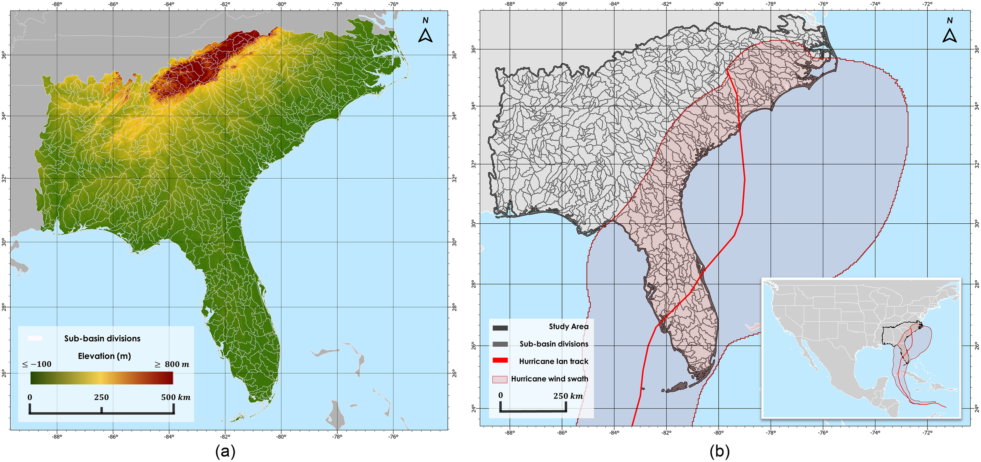
Geographic Area of the Demonstration
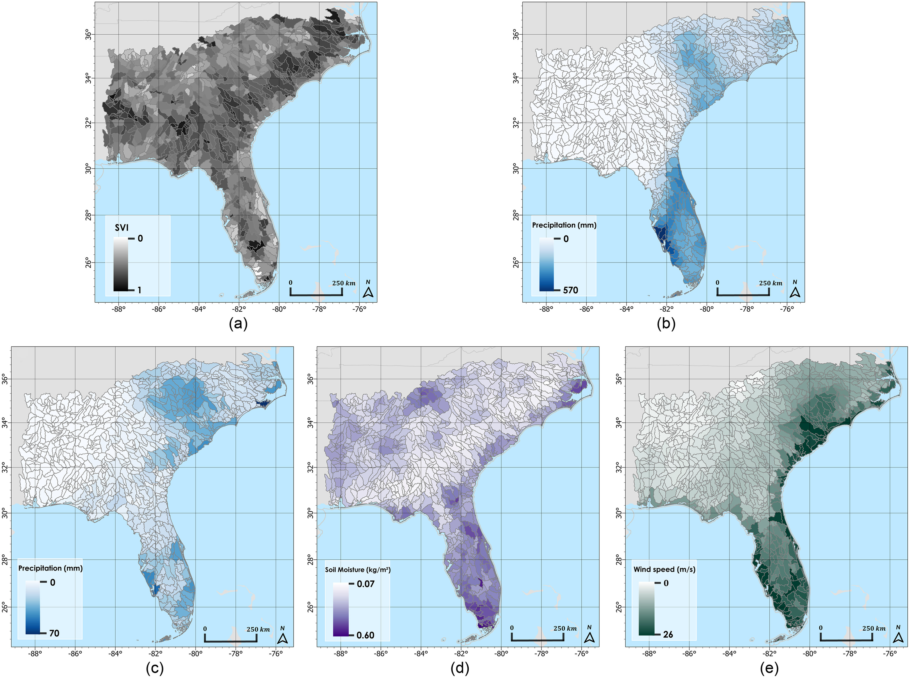
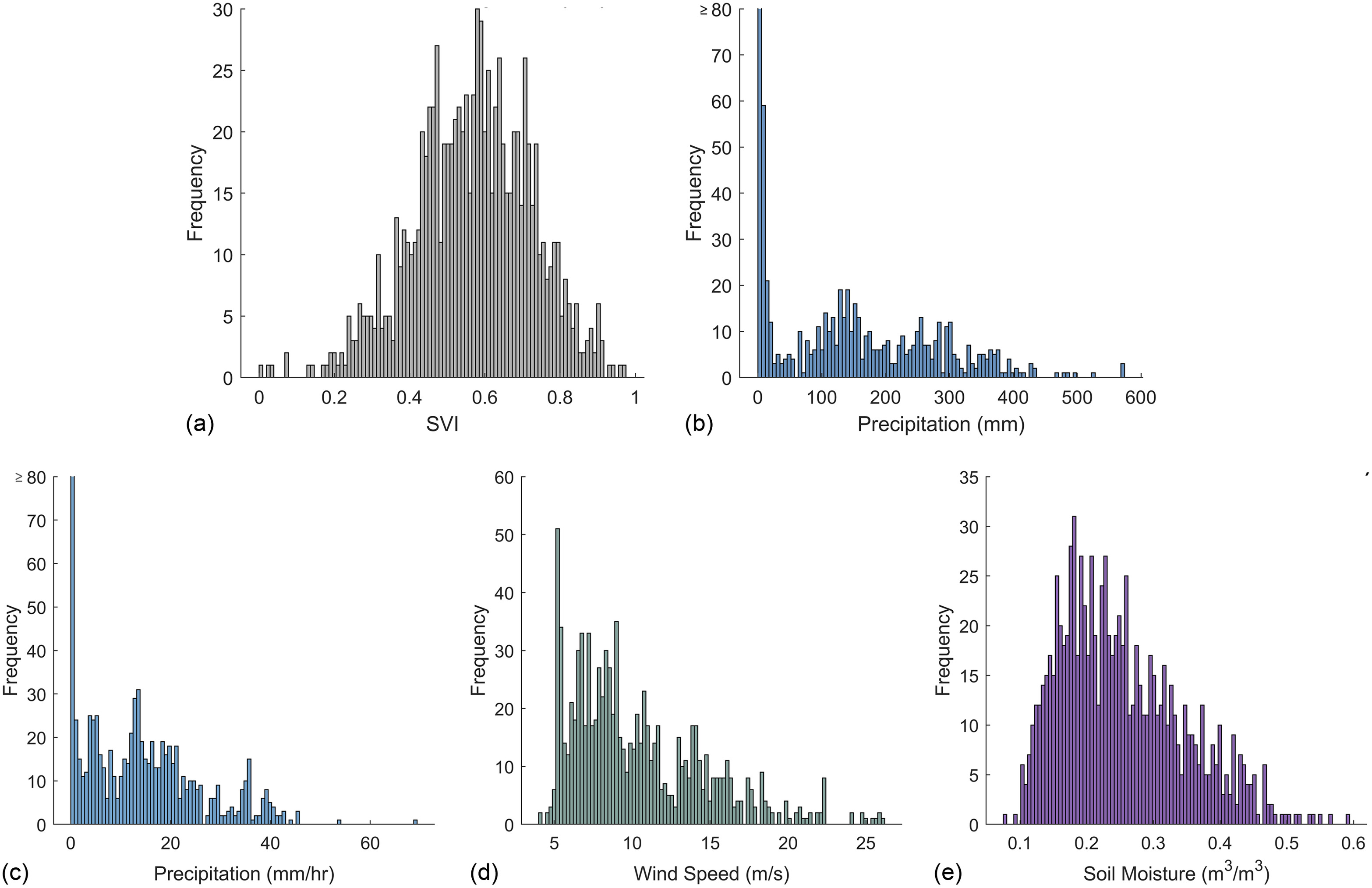
Sources of Data for the Demonstration
| Variable | Sensor/model | Native spatial resolution | Resampled resolution | Resampling method | Temporal resolution | Study period | References |
|---|---|---|---|---|---|---|---|
| Social vulnerability index (SVI) | CDC/ATSDR social vulnerability index 2020 database, US | Census tracks | Level 08 Hydro-BASINS | Spatial average | 1 year | 2020 | CDC/ATSDR (2023) |
| Precipitation | GPM IMERG late precipitation L3 half hour precipitation V06 | 0.1° | Level 08 Hydro-BASINS | Spatial sum and spatial maximum | 1 h | September 27–October 1, 2022 | Huffman et al. (2020) |
| Soil moisture (near-surface, 0–5 cm) | UVA 1-km downscaled soil moisture product | 1-km | Level 08 Hydo-BASINS | Spatial average | 12 h | September 23– September 27, 2022 | Lakshmi and Fang (2023) |
| Wind speed | ECMWF ERA5 | 0.25° | Level 08 Hydro-BASINS | Spatial maximum | 1 h | September 27–October 2, 2022 | Hersbach et al. (2020) |
| Subbasins | HydroBASINS | Level 08 | N/A | N/A | N/A | N/A | Lehner and Grill (2013) |
Subbasin Delineations from HydroBASINS
CDC/ASTDR Social Vulnerability Index
Precipitation Data from GPM IMERG
Wind Speed Data from ECMWF ERA5
SMAP-Derived 1-km Downscaled Surface Soil Moisture Product
Methods
| Scenario () | Swing weights () of contributing variables () | ||||
|---|---|---|---|---|---|
| : SVI | : P1 | : P2 | : W | : SM | |
| : SVI (baseline order) | 1 | 0 | 0 | 0 | 0 |
| : Hurricane Ian cumulative precipitation | 0 | 1 | 0 | 0 | 0 |
| : Hurricane Ian maximum hourly precipitation | 0 | 0 | 1 | 0 | 0 |
| : Hurricane Ian maximum hourly wind speed | 0 | 0 | 0 | 1 | 0 |
| : Hurricane Ian 5-day antecedent soil moisture | 0 | 0 | 0 | 0 | 1 |
| : SVI and Hurricane Ian cumulative precipitation | 0.5 | 0.5 | 0 | 0 | 0 |
| : SVI and Hurricane Ian maximum hourly precipitation | 0.5 | 0 | 0.5 | 0 | 0 |
| : SVI and Hurricane Ian maximum hourly wind speed | 0.5 | 0 | 0 | 0.5 | 0 |
| : SVI and Hurricane Ian 5-day antecedent soil moisture | 0.5 | 0 | 0 | 0 | 0.5 |
| : SVI, Hurricane Ian cumulative precipitation and maximum hourly precipitation | 0.5 | 0.25 | 0.25 | 0 | 0 |
| : SVI, Hurricane Ian cumulative precipitation and maximum hourly windspeed | 0.5 | 0.25 | 0 | 0.25 | 0 |
| : SVI, Hurricane Ian cumulative precipitation and 5-day antecedent soil moisture | 0.5 | 0.25 | 0 | 0 | 0.25 |
| : SVI, Hurricane Ian maximum hourly precipitation and maximum hourly wind speed | 0.5 | 0 | 0.25 | 0.25 | 0 |
| : SVI, Hurricane Ian maximum hourly precipitation and 5-day antecedent soil moisture | 0.5 | 0 | 0.25 | 0 | 0.25 |
| : SVI, Hurricane Ian maximum hourly wind speed and 5-day antecedent soil moisture | 0.5 | 0 | 0 | 0.25 | 0.25 |
| : SVI, Hurricane Ian cumulative precipitation, maximum hourly precipitation, and maximum hourly wind speed | 0.5 | 0.167 | 0.167 | 0.167 | 0 |
| : SVI, Hurricane Ian cumulative precipitation, maximum hourly precipitation, and 5-day antecedent soil moisture | 0.5 | 0.167 | 0.167 | 0 | 0.167 |
| : SVI, Hurricane Ian cumulative precipitation, maximum hourly wind speed, and 5-day antecedent soil moisture | 0.5 | 0.167 | 0 | 0.167 | 0.167 |
| : SVI, Hurricane Ian maximum hourly precipitation, maximum hourly wind speed, and 5-day antecedent soil moisture | 0.5 | 0 | 0.167 | 0.167 | 0.167 |
| : SVI, Hurricane Ian cumulative precipitation, maximum hourly precipitation, maximum hourly wind speed, and 5-day antecedent soil moisture | 0.5 | 0.125 | 0.125 | 0.125 | 0.125 |
Note: Contributing variables include social vulnerability index (SVI), cumulative precipitation (P1), maximum hourly precipitation (P2), maximum hourly wind speed (W), and 5-day antecedent soil moisture (SM).
Sample of Results
Single Variable Basin Order Results
Social Vulnerability Index Order
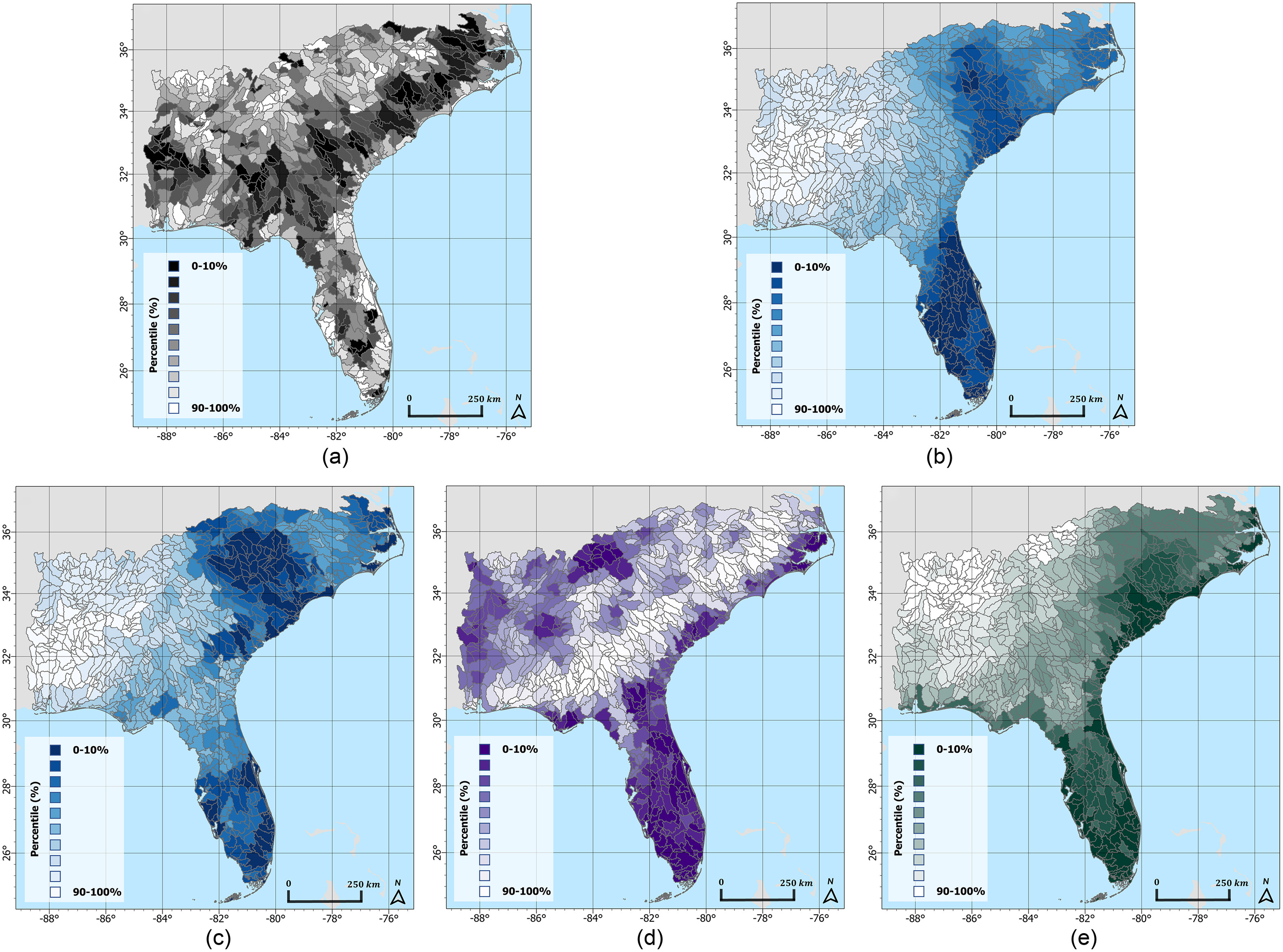
Precipitation (P1 and P2) Orders
Wind Speed (W) Order
Soil Moisture Order
Scenario Results
| Scenario () | Number of basins within a percentage of disruption (%) compared to | |||||||||
|---|---|---|---|---|---|---|---|---|---|---|
| 0%–10% | 10%–20% | 20%–30% | 30%–40% | 40%–50% | 50%–60% | 60%–70% | 70%–80% | 80%–90% | 90%–100% | |
| 196 | 176 | 127 | 101 | 107 | 70 | 53 | 39 | 33 | 20 | |
| 196 | 169 | 128 | 111 | 97 | 80 | 49 | 39 | 34 | 19 | |
| 210 | 178 | 122 | 109 | 109 | 63 | 52 | 31 | 29 | 19 | |
| 166 | 130 | 115 | 118 | 113 | 92 | 75 | 53 | 42 | 18 | |
| 308 | 269 | 167 | 94 | 84 | 0 | 0 | 0 | 0 | 0 | |
| 300 | 274 | 165 | 110 | 70 | 3 | 0 | 0 | 0 | 0 | |
| 322 | 262 | 173 | 104 | 59 | 2 | 0 | 0 | 0 | 0 | |
| 263 | 217 | 182 | 144 | 104 | 12 | 0 | 0 | 0 | 0 | |
| 289 | 297 | 154 | 117 | 65 | 0 | 0 | 0 | 0 | 0 | |
| 326 | 249 | 166 | 126 | 55 | 0 | 0 | 0 | 0 | 0 | |
| 368 | 269 | 164 | 69 | 51 | 1 | 0 | 0 | 0 | 0 | |
| 327 | 254 | 181 | 117 | 43 | 0 | 0 | 0 | 0 | 0 | |
| 371 | 271 | 180 | 71 | 29 | 0 | 0 | 0 | 0 | 0 | |
| 387 | 259 | 168 | 69 | 38 | 1 | 0 | 0 | 0 | 0 | |
| 312 | 271 | 174 | 108 | 57 | 0 | 0 | 0 | 0 | 0 | |
| 320 | 308 | 186 | 80 | 28 | 0 | 0 | 0 | 0 | 0 | |
| 348 | 294 | 176 | 66 | 38 | 0 | 0 | 0 | 0 | 0 | |
| 343 | 310 | 179 | 61 | 29 | 0 | 0 | 0 | 0 | 0 | |
| 335 | 274 | 203 | 80 | 30 | 0 | 0 | 0 | 0 | 0 | |
Basin Ordering for Select Scenarios
| order | Basin name () | State | Basin type | Baseline order () |
|---|---|---|---|---|
| 1 | 7080044390 | FL | Coastal | 10 |
| 2 | 7080044450 | FL | Coastal | 1 |
| 3 | 7080789240 | FL | Inland | 4 |
| 4 | 7080696960 | SC | Inland | 45 |
| 5 | 7080791760 | FL | Inland | 2 |
| 6 | 7080791840 | FL | Inland | 20 |
| 7 | 7080684980 | SC | Inland | 35 |
| 8 | 7080791630 | FL | Inland | 11 |
| 9 | 7080684850 | SC | Inland | 73 |
| 10 | 7080691080 | SC | Inland | 25 |
| 11 | 7080791790 | FL | Inland | 6 |
| 12 | 7080676370 | SC/NC | Inland | 36 |
| 13 | 7080667100 | SC/NC | Inland | 97 |
| 14 | 7080677550 | SC/NC | Inland | 69 |
| 15 | 7080043160 | SC | Coastal | 135 |
| 16 | 7080675620 | SC | Inland | 98 |
| 17 | 7080684690 | SC | Inland | 96 |
| 18 | 7080690650 | SC | Inland | 39 |
| 19 | 7080043100 | SC | Coastal | 147 |
| 20 | 7080675700 | SC | Inland | 142 |
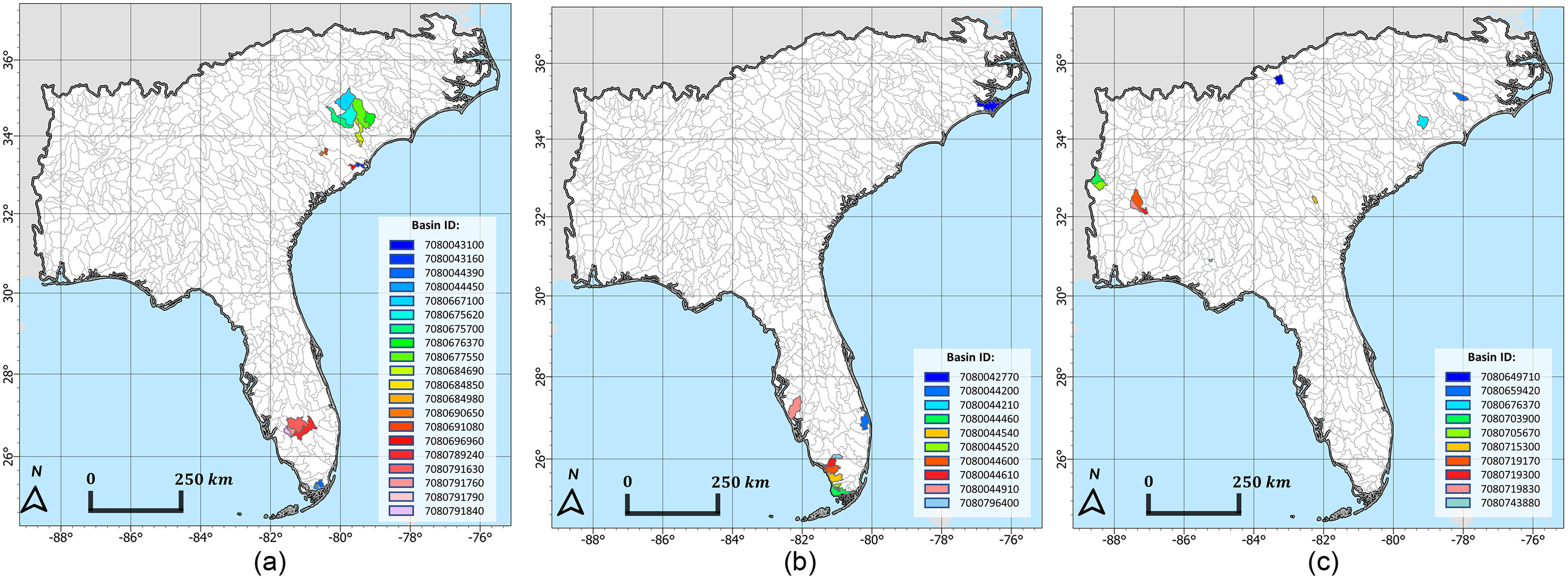
Note: The HydroBASINS Level-08 basin name, state, basin type (coastal or inland), and baseline order () are provided. A reference map of the basin locations is available in Fig. 9(a).
Risk as the Disruption of Basin Order
| Rank of largest increase in priority | Basin name () | Increase in prioritization (%) | Baseline order () | Scenario of minimum order () | Minimum order |
|---|---|---|---|---|---|
| 1 | 7080044540 | 99.35 | 921 | 5 | 5 |
| 2 | 7080044200 | 98.16 | 912 | 3 | 7 |
| 3 | 7080044210 | 98.05 | 913 | 2 | 9 |
| 4 | 7080044520 | 97.94 | 922 | 5 | 19 |
| 5 | 7080044600 | 97.94 | 920 | 5 | 17 |
| 6 | 7080044460 | 97.61 | 901 | 5 | 1 |
| 7 | 7080044610 | 97.51 | 906 | 4 | 7 |
| 8 | 7080044910 | 96.96 | 896 | 2 | 2 |
| 9 | 7080796400 | 95.88 | 893 | 5 | 9 |
| 10 | 7080042770 | 95.01 | 877 | 3 | 1 |
Note: The rank of largest increase in priority, HydroBASINS Level-08 basin name, increase in prioritization percentage, baseline order (), scenario of minimum order, and minimum order are provided for each basin. A reference map is shown in Fig. 9(b).
| Rank of largest decrease in priority | Basin name () | Decrease in prioritization (%) | Baseline order () | Scenario of maximum order () | Maximum order |
|---|---|---|---|---|---|
| 1 | 7080649710 | 23 | 4 | 921 | |
| 2 | 7080719300 | 18 | 2 | 896 | |
| 3 | 7080719830 | 26 | 2 | 897 | |
| 4 | 7080659420 | 33 | 5 | 895 | |
| 5 | 7080676370 | 36 | 5 | 898 | |
| 6 | 7080719170 | 34 | 2 | 894 | |
| 7 | 7080715300 | 14 | 5 | 873 | |
| 8 | 7080705670 | 17 | 2 | 865 | |
| 9 | 7080703900 | 8 | 2 | 855 | |
| 10 | 7080743880 | 85 | 5 | 921 |
Note: The rank of largest decrease in priority, HydroBASINS Level-08 basin name, decrease in prioritization percentage, baseline order (), scenario of maximum order, and maximum order are provided for each basin. A reference map is shown in Fig. 9(c).
Discussion
Machine Learning for Basin-Level Risk Assessment
Validation
Conclusions
| Types of results | Specific results | Comments | Sources |
|---|---|---|---|
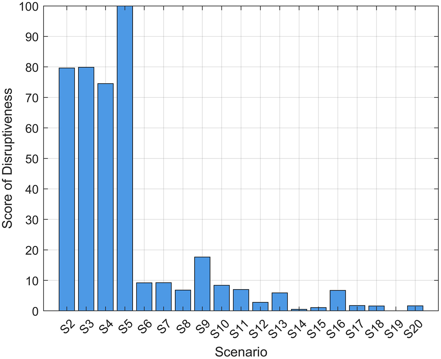
| Most disruptive scenarios | –Hurricane Ian 5-day antecedent soil moisture, | Scenarios of only one contributing variable exhibited the disruptive spatial patterns, relative to the baseline order (). | Fig. 6, Table 3 |
| –Hurricane Ian maximum hourly precipitation, | |||
| –Hurricane Ian cumulative precipitation | |||
| Least disruptive scenarios | –SVI, Hurricane Ian maximum hourly precipitation, maximum hourly wind speed, and 5-day antecedent soil moisture | Scenarios of four hydrology and social variables resulted in spatial patterns that were least disruptive to the baseline order (). | Fig. 6, Table 3 |
| –SVI, Hurricane Ian cumulative precipitation, maximum hourly wind speed, and 5-day antecedent soil moisture | |||
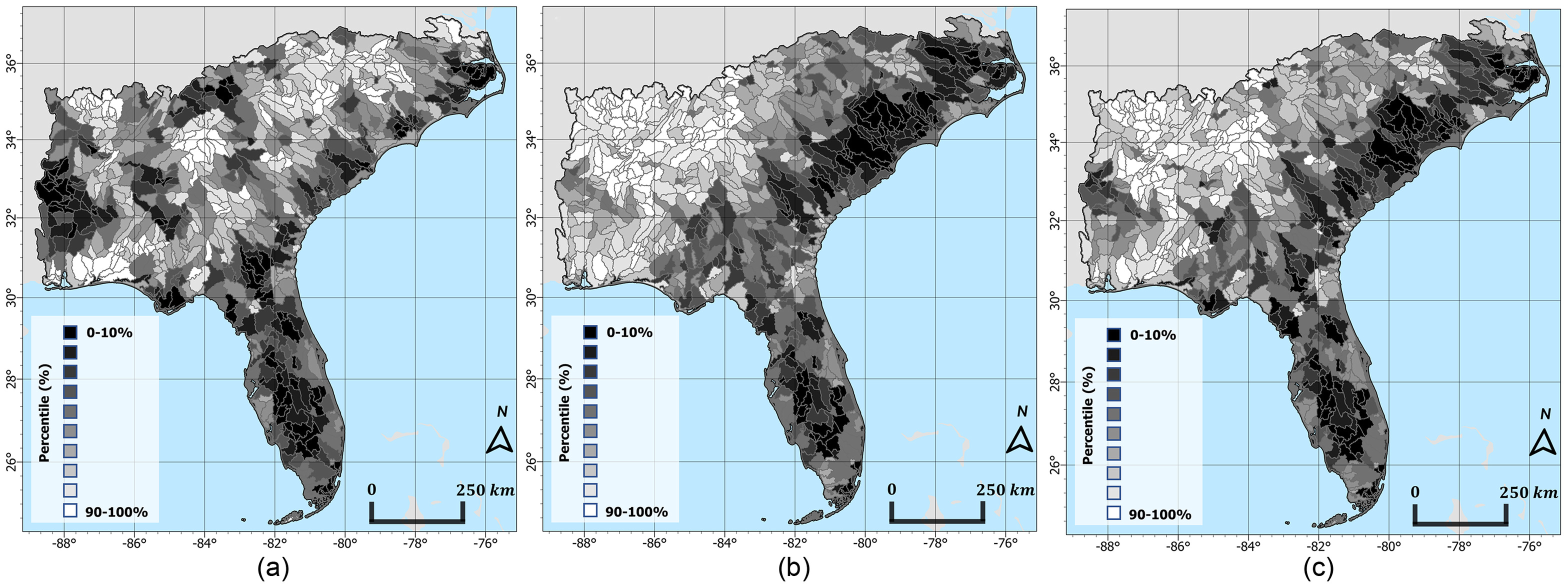
| Highest priority basins in disrupted orders | Inland basins of Florida and South Carolina followed by coastal basins of Florida, South Carolina, and North Carolina | Basins of high social vulnerability located within the hurricane path were exposed to the most extreme hydrological conditions and may be prioritized for near-term recovery, response, and future mitigation efforts. | Fig. 7, Table 4, Fig. 9(a) |
| Lowest priority basins in disrupted orders | Alabama and North Georgia basins | Basins of low social vulnerability located outside the hurricane path had low priority. | Figs. 7 and 8 |
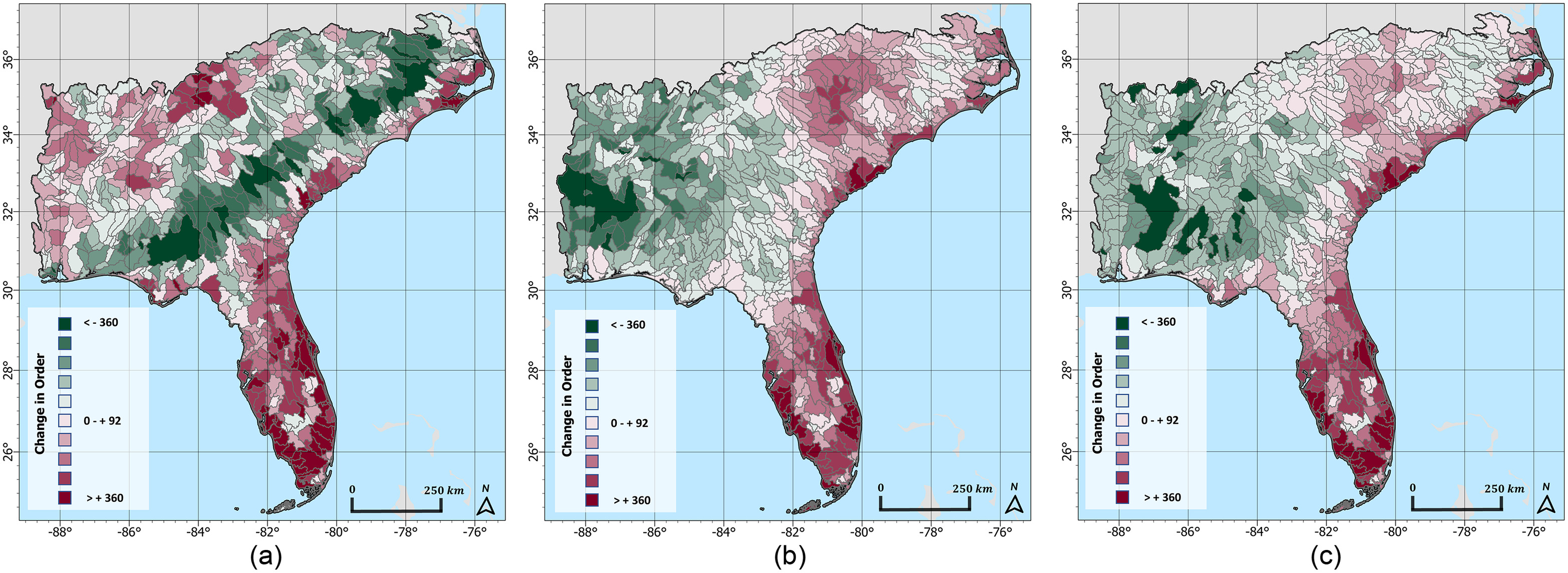
| Greatest increase in basin priority | Coastal basins of Florida | These basins had very high exposure to hydrological conditions during Hurricane Ian but low social vulnerability in the baseline order. They are protected wetlands, nature preserves, parks, and affluent communities with low social vulnerability. | Fig. 8, Table 5, Fig. 9(b) |
| Greatest decrease in basin priority | Inland basins of Alabama, South Carolina, and North Carolina | These basins had the highest social vulnerability in the baseline order but were located outside the hurricane path, meaning they had low hydrological exposure. | Fig. 8, Table 6, Fig. 9(c) |
Notation
- cumulative precipitation;
- maximum hourly precipitation;
- risk; the difference between the baseline order and scenario order of a given basin;
- 5-day antecedent soil moisture;
- basin order using social vulnerability index data; the baseline order;
- -component of wind in the longitudinal direction 10 m above the surface of the Earth;
- maximum hourly wind speed;
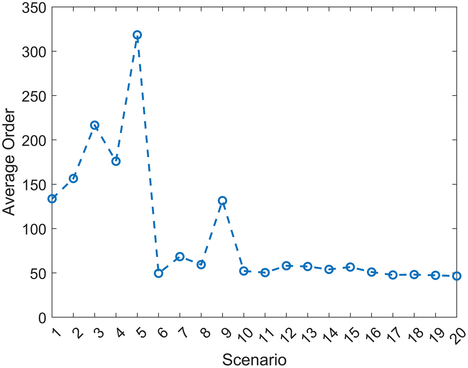
- normalized score of disruptiveness for a given scenario (); the score of disruptiveness for a given scenario minus the minimum score of disruptiveness () divided by the maximum score of disruptiveness () minus the minimum score of disruptiveness (); and
- score of disruptiveness for a given scenario (); the sum over the basins of the squared differences of the baseline order and disrupted order.
Appendix I. Examples of Tropical Cyclone Disaster Challenges Associated with Social Vulnerability
Appendix II. Summary of Themes and Variables Contributing to Census-Tract Level Social Vulnerability Index Calculation
| Themes | Variables |
|---|---|
| Socioeconomic status | 1. Below 150% poverty 2. Unemployed 3. Housing cost burden 4. No high school diploma 5. No health insurance |
| Household characteristics | 1. Aged 65 and older 2. Aged 17 and younger 3. Civilian with a disability 4. Single-parent households 5. English language proficiency |
| Racial and ethnic minority status | 1. Hispanic or Latino (of any race) 2. Black and African American, not Hispanic or Latino 3. American Indian and Alaska Native, not Hispanic or Latino 4. Asian, not Hispanic or Latino 5. Native Hawaiian or other Pacific Islander, not Hispanic or Latino 6. Other races, not Hispanic or Latino |
| Housing type and transportation | 1. Multiunit structures 2. Mobile homes 3. Crowding 4. No vehicle 5. Group quarters |
Source: Data from CDC/ATSDR (2023).
Appendix III. Data Sets Used for Demonstration of the Methodology for Hurricane Ian
HydroBASINS
GPM IMERG
ECMWF ERA5
SMAP-Derived 1-km Downscaled Surface Soil Moisture Product
Data Availability Statement
Acknowledgments
References
Information & Authors
Information
Published In

Copyright
History
ASCE Technical Topics:
- Basins
- Bodies of water (by type)
- Business management
- Climates
- Construction engineering
- Construction management
- Disaster risk management
- Disasters and hazards
- Environmental engineering
- Hurricanes, typhoons, and cyclones
- Hydrologic engineering
- Hydrology
- Meteorology
- Natural disasters
- Practice and Profession
- Precipitation
- Project management
- Resource allocation
- Risk management
- Social factors
- Storms
- Water and water resources
- Water management