Quantifying Social Inequalities in Flood Risk
Publication: ASCE OPEN: Multidisciplinary Journal of Civil Engineering
Volume 2, Issue 1
Abstract
The distribution and inequalities of flood risks across space and social groups are important considerations for infrastructure design and adaptation. However, neither civil infrastructure practitioners nor researchers routinely assess inequalities quantitatively, which limits opportunities to address them. The Lorenz curve method has been used in many fields to study inequalities in both resource and risk distributions across populations, and it supports a quantitative measure of inequality, the Gini index. Here we present the formulation of Lorenz curves and a data analysis workflow to measure inequalities in both flood damages and flood exposure using flood hazard, flood damage, and social data. We define flood exposure as flood depth multiplied by population density, whereas flood damages are taken strictly as a measure of economic losses. We then show that Lorenz curves for flood damages have the potential to differ markedly from Lorenz curves for flood exposure since the latter is dependent on the population density. For example, higher population density reduces per person damages but increases total flood exposure. Furthermore, we illustrate the Lorenz curve method at scale with an application to Los Angeles County, home to nearly 10 million people. These results demonstrate both similarities and differences between flood damage and flood exposure inequalities for different racial and ethnic groups, and they also show that regional inequalities are sensitive to changes in flood severity and the capacity of flood infrastructure. These sensitivities illuminate the complexity of achieving social equality in flood adaptation, and they emphasize both the utility of detailed modeling and the need for community-engaged decision-making to evaluate and implement response measures. A review of state and federal flood assistance programs reveals heightened opportunities to shape public investments with quantitative measures of flood risk inequalities.
Introduction
Flood control infrastructure including dams, levees, and drainage systems have been instrumental in enabling and supporting global economic development and public safety (Mach et al. 2022). Lowland topography naturally exposed to flooding, including river floodplains and deltas, has been reclaimed and converted for agricultural and industrial needs over many centuries (Andreadis et al. 2022), and residents, businesses, and municipalities alike are now dependent upon flood risk management efforts to reduce the likelihood of flood waters damaging assets, threatening lives, and displacing people (Barry 1997; Molinaroli et al. 2019; Montz and Gruntfest 1986; Brody et al. 2007).
However, the benefits of flood control and risk management have not been shared equally (e.g., Wing et al. 2022; Glavovic et al. 2022; Shi 2021). First, flood hazards are unevenly distributed across populations. These patterns have been observed within cities (e.g., Debbage 2019; Sanders et al. 2023) and across the U.S. (e.g., Wing et al. 2022; Vahedifard et al. 2023). Recent flood damages, of 32.1 billion USD annually on average, have disproportionately impacted poorer communities, and future climate change through to 2050 is projected to increase flood risk by 26% across the U.S. and disproportionately affect Black communities (Wing et al. 2022). Second, flooding can compound underinvestment in communities and disproportionately impact households that are already marginalized and underserved. These compounding and cascading impacts, for example, result from differential displacement and subsequent returns following flooding or the postdisaster challenges of recovery and rebuilding amid housing scarcity and prolonged impacts on livelihoods and well-being (Mach et al. 2022). Third, flood risk-management and disaster-recovery policies can themselves contribute to inequities (Billings et al. 2022; Domingue and Emrich 2019; Hornbeck and Naidu 2014; Smiley 2020). For example, neighborhoods and communities with higher wealth, and lower racial and ethnic diversity have been more likely to receive government grants and investments supporting flood risk reduction, disaster relief, and rebuilding (Mach et al. 2019; Bullard and Wright 2012; Tate et al. 2016; Siders and Keenan 2020). Fourth, recent initiatives encouraging adaptive action have emphasized increasing participation in decision-making processes, with less success in actual, substantive transformations toward improved distributions of risks and policy benefits (Shi 2021).
Broadly speaking, it seems reasonable for the public to expect the government to provide a baseline of safety for environmental risks such as flooding. However, the demands on infrastructure are increasing with climate change and compounding flood hazards (Milly et al. 2008; Hino et al. 2019), and priorities for flood infrastructure are multifaceted (Kousky 2015; Glavovic et al. 2022; England and Knox 2015). Among diverse related goals, communities need a reliable water supply and seek benefits such as water-based recreation, healthy ecosystems, and cohesive and connected societies. Communities also need adaptive investments in the face of other climate-related hazards, such as shade and cooling to reduce the risks of extreme heat and defensible open space to reduce risks from wildfire. Further, communities expect governments to fairly deliver these services and benefits, but as the aforementioned demands on public infrastructure grow, it is plausible that inequities will worsen. All of this is in a context of rising economic inequalities in the U.S. and many other countries (Brady et al. 2016). A more sophisticated understanding of how to measure social inequalities is thus becoming more salient for engineering and public infrastructure analyses, decision making, and problem solving.
For a very long time, scholars of inequalities in economic resources (e.g., on income, earnings, and wealth) have developed a variety of approaches for measuring inequality, and these approaches can feasibly be applied to measure social inequalities in flood risks including threats to safety and economic losses. One of the most common metrics, the Gini index, quantifies how much a given community or society departs from perfect equality, and has typically been used in the context of income inequality (Lorenz 1905). Whereas in a perfectly equal society, resources and risks are distributed proportionately to population, most societies depart from perfect equality, and advantaged members receive a disproportionate share of resources or disproportionate protection from risks. The actual distribution is measured with what is called a “Lorenz curve,” and the Gini index quantifies how much the Lorenz curve departs from perfect equality (Lorenz 1905).
To illustrate how the Gini index is computed from data, consider an example of ten people with different income and ages as in Figs. 1(a and b), respectively. To measure income inequality, we sort the individuals by increasing income [Fig. 1(c)] and then plot the normalized cumulative distribution of income versus the normalized cumulative number of individuals to arrive at the Lorenz curve [Fig. 1(e)]. The Gini index subsequently follows as the departure from perfect equality [1:1 line on Fig. 1(e)], specifically, twice the shaded area in Fig. 1(e) and here given by 0.28 – a moderate level of inequality. The Gini index can range from to 1, and values of zero correspond to perfect equality. However, more powerfully, the Gini index can also quantify inequality relative to social factors such as age, race, ethnicity, and disadvantage. Fig. 1(d) depicts the distribution of income across individuals after sorting by increasing age, and Fig. 1(e) depicts the corresponding Lorenz curve. In this case, the Gini index is small (0.06) which suggests that income is not disproportionately higher among older individuals. In fact, the “S” shape of the Lorenz curve points to an increase in income with age among the younger individuals, and a decrease in income with age among older individuals, as suggested by the distribution of income in Fig. 1(d).

However, use of Lorenz curves and Gini indices in studies of flood risk inequalities has been limited. For example, Bin et al. (2012) examined whether the National Flood Insurance Program (NFIP) favored wealthier counties of the U.S. by using Gini indices of county-average income, premiums, and payouts – finding that the program was at most mildly progressive, with no evidence of advantages for wealthier counties. Ciullo et al. (2020) integrated equity considerations into cost–benefit analyses of flood mitigation options using a Gini index, which measured differences in costs (e.g., flood damages) between regions. Lindersson et al. (2023) investigated flood mortality in relation to income inequality as measured by a Gini index. Flood exposure and flood loss inequalities have also been analyzed with metrics other than Gini indices. Chakraborty et al. (2014) analyzed trends in flood hazard levels at the census tract scale relative to explanatory factors including race and ethnicity to assess inequalities. Wing et al. (2022) presented histograms of losses across census tracts sorted by racial/ethnic population to explore inequalities. Debbage (2019) used risk ratios given by the share of one social group at risk of flooding relative to the share of another group at risk of flooding. Messager et al. (2021) used flood exposure representativeness (FER), the share of a population group within a flood zone relative to the share of that same group in the reference population (e.g., Maantay and Maroko 2009). Schroder et al. (2022) also focused on the share of population of social groups in the flood zone relative to a reference group. Recent studies have also shown that flood risk inequalities are sensitive to flood magnitude (Selsor et al. 2023; Sanders et al. 2023).
Sanders et al. (2023) introduced the measurement of flood exposure inequalities with a Gini index but did not consider inequalities in flood damages. We will show here that Lorenz curves for economic losses are formulated differently than Lorenz curves for flood exposure, and we will provide novel evidence that Lorenz curves for flood damage have the potential to differ markedly from Lorenz curves for flood exposure. Indeed, a methodological foundation for applying the Gini index to flood risk calls for attention to both flood exposure and flood losses, and the objective of this paper is to provide an introduction to the method with background and illustrative examples highlighting important sensitivities. Furthermore, the paper aims to highlight opportunities to systematically integrate social inequality metrics into flood adaptation. More generally, this piece provides a forward-looking methodological and conceptual framework for future analyses of inequities in flood risks.
This paper is organized into three sections. In the first section, we present the formulation of the Lorenz curve and Gini index to measure two different types of flood risk inequalities: damage inequalities and exposure inequalities. The notion of exposure here captures the potential for flood hazards to impact human safety and well being, which increases with increasing flood depth, while damage is represented by an econometric function that could depend on many different factors including flood depth. In the second section, we present a case study of damage and exposure inequalities at scale, exploring the sensitivity of inequalities to flood magnitude and infrastructure capacity. The third section describes opportunities to integrate inequality data into decision-making processes that shape flood adaptation.
Lorenz Curve and Gini Index for Flood Risk Inequalities
As mentioned previously, the Lorenz curve and Gini index are tools to measure the departure of a resource (or a risk) from a distribution that is proportional to the population. It bears emphasizing that the Gini index measures an inequality – strictly a measure of the uneven distribution across the population – and not inequity, which often implies fairness or social justice or mobility or opportunity. For example, differences in salaries are common within most organizations and represent an inequality but not necessarily an inequity, due to differences in skills, experience, and capacity. This highlights the importance of using equity-based frameworks alongside inequality measurements to understand the root causes of inequality and develop solutions that are tailored to the specific circumstances of communities (Howard and Wilkes 2022).
The development of a Lorenz curve for flood risk inequalities requires data describing the spatial distribution of population, flood hazards, flood damage estimates, and social factors such as race, ethnicity, and disadvantage. Reconciling these data at the same scale, or unit of analysis, is the starting point for inequality analysis.
Unit of Analysis
In the U.S., population and social data are provided by the U.S Census (US Census Bureau 2020a) and American Community Survey (US Census Bureau 2020b). Census data are available at varying sizes of geographical units, including Census Tracts (1,200–8,000 people), Block Groups (600–3,000 people), and Blocks (US Census Bureau 2022), and the block-group scale is the finest available for social data useful for this analysis. Flood hazard data such as flood depth and velocity are produced by simulation models, and the available resolution will depend on the computational grid. Across the U.S., nationwide data have been generated at a resolution of 30 m (Bates et al. 2021), and more detailed models with a resolution of 3 m resolution have been produced regionally (Sanders et al. 2023). Flood zones delineated by the Federal Emergency Management Agency (FEMA) have also been used in equity analysis (Debbage 2019; Messager et al. 2021), but these maps tend to underestimate areas at risk (Wing et al. 2018; Sanders et al. 2023). Flood hazard models that account for stormwater infrastructure (e.g., levees, culverts, drain pipes) and resolve detailed patterns of topography (<5 m) are especially important for accuracy in urban areas where population density is high and nationwide models are less reliable (Wing et al. 2017; Kahl et al. 2022; Bates 2023). Flood damage (or loss) data follows from additional modeling that considers the assets exposed to flooding and their susceptibility to losses from flooding (FEMA 2022b). In the U.S., damage modeling is now supported nationwide by the National Structure Inventory developed by the U.S. Army Corps of Engineers (USACE 2022), and the Hazus program developed by the Federal Emergency Management Agency (FEMA 2022b). Moreover, previous research has suggested that damage modeling introduces considerable uncertainties from limitations of the structural inventory (Sanderson and Cox 2023) and models describing the susceptibility of buildings to losses (Wing et al. 2020).
The best unit of analysis to reconcile data for inequality analysis is likely to vary depending on the type of inequality analysis sought (exposure versus damage), the availability of data across scales, and geographic factors such as population density and flood hazard variability. Tate et al. (2021) reconciled data at the scale of census tracts for flood exposure and vulnerability analysis across the conterminous U.S., using 30 m resolution hazard and land cover data to inform estimates of exposed population. Sanders et al. (2023) reconciled data at the scale of land parcels to assess exposure inequalities across Los Angeles County. Similarly, Messager et al. (2021) reconciled data at the scale of land parcels in Washington State and emphasized the importance of a fine-scale approach for assessment of exposed populations and inequalities. Indeed, urban flooding is typically characterized by flood depths (and exposure) that change substantially across land parcels and roadways, and from city block to city block (Schubert et al. 2022), and thus fine-grained data can be expected to better capture spatially heterogeneous hazards and exposure. Land parcels are especially informative for urban areas of the U.S. because they are the scale at which property value data and land use information are archived by local governments, they are the scale of ownership for property data, and they are sufficiently small to capture variability in urban flooding.
Outside the U.S., governments adopt different approaches to segment the population but can be expected to have population, social, and land use information available at a range of scales. Inequality analysis will nevertheless require the identification of spatial units over which the covariability of population, flood hazard, flood loss, social, and other relevant data are captured.
Data processing is typically required to align data with a common unit of analysis. In the case of population data, dasymetric population estimation refers to the estimation of population and social information at finer scales than available with Census data, using information about land use and/or building types. Typically, the population measured at the scale of a census unit (e.g., block group) is distributed across land parcels classified as residential in a way that is informed by land parcel data such as the size of the land parcel or the building type (Debbage 2019; Messager et al. 2021). Moreover, we assume that every land parcel has the proportionate demographic statistics (e.g., racial and ethnic fractions) of the census unit in which it is embedded. This serves as a reminder that when estimating population and demographic statistics at the scale of individual land parcels, some of the variables will correspond to averages representative of larger (e.g., neighborhood) scales, and the predictive power of the data will be for neighborhood and larger scales. Estimation of flood hazards by land parcel is comparatively straightforward. Hazards are estimated for each unit of analysis by averaging or sampling simulation data from a grid (Tate et al. 2021; Sanders et al. 2023). Loss estimation at the parcel scale becomes possible given the availability of building stock data and flood hazard data at the same scale (FEMA 2022b).
Building the Lorenz Curve
The workflow to create a Lorenz curve was illustrated in Fig. 1 for a case of income inequality across individuals, and here we describe how this approach is extended for flood risk applications, where populations and assets are distributed across a geographical area and vulnerable to flooding. We begin by considering a spatial domain that is subdivided into units with population , flood hazard , flood damage , and a general socioeconomic variable (e.g., racial and ethnic fractions, property values, income) for . Lorenz curve analysis begins by creating an table, , where the first column corresponds to population data, the second column corresponds to either damage data or hazard data (for an estimate of damage or exposure inequities, respectively), and the third variable corresponds to a socioeconomic variable.
Flood Damage Inequality
To estimate flood damage inequality, is first constructed as follows:where , , and are column vectors of length with elements , , and , respectively.
(1)
Second, the rows of the table, , are sorted based on increasing values of the socioeconomic variable . This may represent one of many different variables such as population fractions of race and ethnicity, income, property values, and measures of disadvantage. We express the sorting process, based on elements of arranged in ascending order, as follows:The sorted table produces sorted vectors of population data and damage data , which are then used to compute cumulative distribution functions as follows:and normalized distributions as follows:for which results in both and varying from 0 to 1.
(2)
(3)
(4)
The flood damage Lorenz curve corresponds to cumulative damage, , versus cumulative population, . To illuminate both equal and unequal distributions of flood damage, Fig. 2 depicts flood damage Lorenz curves for four canonical distributions of population and hazard: (a) a spatially uniform population density and damage distribution; (b) a spatially uniform population density and linearly varying damage distribution (across units of analysis); (c) a linearly varying population density (across units of analysis) and spatially uniform damage distribution; and (d) a population density and damage distribution that both linearly increase across units of analysis. The sorting step in the Lorenz curve development given by Eq. (2) is implemented by taking either flood damage or population density as the sorting variable, whichever is linearly increasing. Fig. 2 depicts the variation in damage across the population with background color (low damage in turquoise, high damage in pink), and the variation in population density with the background circle size.

In the first case [Fig. 2(a)], the proportion of the damage increases linearly with the proportion of the population, which corresponds to the line of equality. In the second case [Fig. 2(b)], the Lorenz curve falls below the line of equality to indicate an inequality in flood damage, i.e., flood damage falls disproportionately across the population. As mentioned previously, the Gini index, , is given by the ratio of the shaded area in Fig. 2(b) divided by the area under the line of equality which can be computed using the trapezoidal rule as follows:With this implementation, the Gini index can vary from to 1 with a value of 0 representing an equality, a positive value indicating an inequality whereby the upper half of the distribution experiences a proportionally greater share of the hazard, and a negative value indicating an inequality whereby the upper half of the distribution experiences a proportionally smaller share of the hazard.
(5)
Fig. 2(c) presents a particularly informative case whereby the population density increases linearly across the flood zone while the flood damages are uniform. Physically, this case could be interpreted as a floodplain with a spatially uniform flood hazard and a rural to urban gradient in land use and land cover. Since damages are greater on a per person basis within areas of less population density, the Lorenz curve tracks above the line of equality and the Gini index is negative. Furthermore, moving on to Fig. 2(d) where population density increases linearly and flood damages increase linearly across the domain, the Lorenz curve indicates perfect equality, which is consistent with damages per person being equal across the population.
Flood Exposure Inequality
To estimate flood exposure inequality, the data table is assembled with population, depth, and social data as follows:and the table is sorted based on increasing values of the variable to yield . The sorted population data are next used to compute the cumulative distribution functions of population and flood exposure (defined as ) as follows:and normalized distributions are computed asfor . Furthermore, the Gini index for flood exposure follows as
(6)
(7)
(8)
(9)
We note that the key difference between the Lorenz curve for flood damages, compared with flood exposure, is the formulation of the axis. In the case of flood damage, the axis corresponds to the cumulative distribution of flood damage, while in the case of flood exposure, the axis corresponds to the cumulative distribution of flood depth multiplied by population density. Hence, the latter involves population weighting.
When population density and flood hazard are uniform across units of analysis, the Lorenz curve falls along the line of equality [Fig. 3(a)] indicating that there is equality in flood exposure across the population. Additionally, when the level of hazard varies across a population, there are inequalities in flood exposure as indicated by Fig. 3(b). Perhaps somewhat surprisingly, there is also equality in flood exposure when the hazard across a population is uniform while the population density is varied, as in Fig. 3(c). Furthermore, across a flood plain where population density and hazard levels are varying, inequalities in exposure are also expected, as in Fig. 3(d).

We stress here that the Lorenz curves for flood damage (Fig. 2) and flood exposure (Fig. 3) exhibit different types of curvature (with implications for inequalities) across four very similar scenarios: either uniform or linear variations in population density and either flood damage or flood hazard depth. For example, the third case involving a linearly varying population density points to inequality in flood damage [Fig. 2(c)] but equality in flood exposure [Fig. 3(d)]. Additionally, the fourth case involving a linearly varying population density points to equality in flood damage [Fig. 2(d)] and inequality in flood exposure [Fig. 2(d)]. These differences stem from population-weighting of the flood depth for the case of flood exposure to create the axis of the Lorenz curve, while there is no weighting of damage data.
Measuring Changes in Inequalities
Changes in inequalities from an intervention (e.g., raising levees, levee setbacks, reservoir construction, buyouts) or climate change can be measured by differences in the Gini index:
(10)
In the social sciences, the terminology Gini index is typically used for a measure of income or economic inequality. Relatedly, the concentration index, , has been used to measure inequalities in the distribution of taxes or benefits. For instance, scholars assess whether the poor receive a disproportionate share of benefits (i.e., low-income targeting) or the rich pay a disproportionate share of taxes (i.e., tax progressivity) (Brady and Bostic 2015). Moreover, differences between the concentration index and the Gini index are termed the Kakwani index (Kakwani 1977):and in the context of taxation, a positive indicates progressive tax measures and a negative indicates regressive measures. When plotting Lorenz curves for income and taxation, the Kakwani index is equal to twice the area falling between the two curves.
(11)
Use of Lorenz curves for inequality analysis has expanded to many different fields where the terminology Gini index is not strictly reserved for economic inequalities, similarly, the Kakwani index has been used to describe differences in Gini indices [Eq. (10)]. In the context of flood risk applications, evaluation of the Gini index given by Eqs. (5) or (9) will invariably reveal that some social groups are disproportionately overexposed (positive Gini index) while other social groups are disproportionately underexposed (negative Gini index) because the occurrence of exposure inequalities is now recognized to be pervasive (Bates 2023). Furthermore, unless the spatial distribution of social groups in an area markedly changes, interventions that reduce inequalities () for some social groups will increase them for others (). Hence, the targeting of flood risk interventions to reduce the disproportionate overexposure faced by some social groups will be accompanied by reductions in the disproportionate underexposure by other social groups.
Flood Exposure and Inequalities in Los Angeles
Los Angeles (LA) County, California is home to a population of 9.8 million people (U.S. Census Bureau) and a gross domestic product of 712 billion USD (U.S Bureau of Economic Analysis), making it larger than 40 U.S. states by population and 43 by economic output. With urban development blanketing a coastal plain below steep mountains rising to over 3,000 m above sea level (Fig. 4), the southern part of LA County is vulnerable to flooding disasters from atmospheric river rainfall events that generate fast-moving runoff and floodwater filled with mud and debris that may overwhelm infrastructure (Jones 2019; Sanders and Grant 2020; Ulibarri et al. 2023).

Fig. 4. Distribution of population density across southern Los Angeles County, California, USA. Flood channels with levees (gold) and without levees (blue) are relied upon for drainage.
[Base map from ArcGIS World Terrain Base (WGS84), Sources: Esri, TomTom, Garmin, FAO, NOAA, USGS, © OpenStreetMap contributors, and the GIS User Community; ArcGIS Multidirectional Hillside, Sources: Airbus, USGS, NGA, NASA, CGIAR, NLS, OS, NMA, Geodatastyrelsen, GSA, GSI, and the GIS User Community.]
Recent research suggests that between 197,000 and 874,000 people (median 425,000) and between 36 billion USD and 108 billion USD in property (median 56 billion USD) currently fall within the 1%-annual chance-flood zone (based on a depth tolerance of 30 cm). Such risk levels far exceed federally defined floodplains and portend similar risks as compared to the most damaging hurricanes in US history (Sanders et al. 2023). Moreover, previous research has indicated that flood exposure corresponding to the 1%-annual-chance event is concentrated within Black and Hispanic communities (Sanders et al. 2023). Heightened flood exposure to the 1%-annual-chance event is attributed to the significance of pluvial flooding in a region marked by expansive urban development and main stem drainage channels that are undersized to contain flood peaks which results in channel overtopping and floodplain inundation (Sanders et al. 2023; Ulibarri et al. 2023).
Here we combine population data, flood hazard data, flood damage data, and social data available from the U.S. Census to illustrate Lorenz curves in both flood damages and flood exposure by social groups, and to compute Gini indices representative of inequalities. Specifically, we develop flood damage Lorenz curves [ versus from Eq. (4)] to compute using Eq. (5), and we develop flood exposure Lorenz curves [ versus from Eq. (8)] to compute using Eq. (9).
Four different scenarios are considered to illustrate two major uncertainties in flood risk: the severity of the flood and the capacity of infrastructure. All four scenarios are interpretations of the 1%-annual-chance fluvial hazard, which is the most widely used hazard scenario for risk mapping in the U.S. and the basis for the National Flood Insurance Program. The first three scenarios capture differences in flood magnitude based on low-end, most-likely, and high-end estimates of the 1%-annual-chance fluvial hazard defined by the 5th, 50th, and 95th percentile, respectively, and are based on the existing capacity of flood infrastructure. The fourth scenario captures an increase in infrastructure capacity, i.e., flood mitigation, and is paired with the most-likely estimate (50th percentile) of the 1%-annual-chance fluvial flood peaks. The mitigation scenario is implemented by assuming that levees along mainstem flood channels (gold coloring in Fig. 4) are raised by one meter. The purpose here is not to advocate for higher levees as a specific solution to address flooding, but rather to illustrate use of the Lorenz curve and Gini index to measure changes in the Gini index, , from a mitigation measure. There is a history of raising levees in the region to contain flood peaks that increase over time with land use change (Orsi 2004), and thus our mitigation scenario is representative of the approach that has been most commonly used historically.
Land Parcel Exposure Dataset
A land parcel shape file dataset with distinct parcels was accessed from Los Angeles County (Los Angeles County 2022) for the assembly of population data, social data, flood hazard data, exposure data, and damage data for subsequent analysis. The parcel dataset included lot area, land use, and property value as well as a polygon for the lot perimeter. Population was estimated dasymetrically by apportioning the block group population from the 2020 Census (US Census Bureau 2020a) across residential parcels in proportion to lot area (Tate et al. 2021), and zero population was ascribed to commercial or other parcel types. Each residential parcel was also assigned a Black, Hispanic, Asian, and White population fraction computed from Census data. Specifically, block group population counts reported by race (Black, Asian, and White) and ethnicity (Hispanic) were divided by the total block group population to determine population fractions that were assigned to each land parcel, as in Fig. 5. Race and ethnicity fractions are not meant to be accurate at the scale of land parcels but allow for meaningful measures of risks and inequalities when aggregated with hazard and damage data at spatial scales greater than block groups. Note that race and ethnicity are distinct in the U.S. Census, and respondents may report combinations of ethnicity and race (e.g., Hispanic and Black). The study area population is 9,105,286, which by ethnicity is 48.2% Hispanic and by race is 49% White, 22.0% other, 14.2% Asian, 8.6% Black, 4.4% Two or More Races, 0.7% Native American, and 0.3% Hawaii and other Pacific Islander.

Fig. 5. Los Angeles County distribution of (a) Black; (b) Hispanic; (c) Asian; and (d) White population fractions. Black, Asian, and White correspond to U.S. census data on race alone, while Hispanic corresponds to U.S. census data on ethnicity. Note that there is overlap between race and ethnicity.
[Base maps from ArcGIS World Terrain Base (WGS84), Sources: Esri, TomTom, Garmin, FAO, NOAA, USGS, © OpenStreetMap contributors, and the GIS User Community; ArcGIS Multidirectional Hillside, Sources: Airbus, USGS, NGA, NASA, CGIAR, NLS, OS, NMA, Geodatastyrelsen, GSA, GSI, and the GIS User Community.]
Flood Hazard Modeling
Flood hazards were modeled using a previously developed and validated Parallel Raster Inundation Model (PRIMo) that resolves flood inundation from pluvial, fluvial, and coastal hazards at 3 m resolution across a 6,804 km2 domain including parts of Los Angeles County and Orange County (Sanders et al. 2023). PRIMo simulates flooding by solving the full shallow-water equations with a dual-grid, Godunov-type finite volume scheme that achieves ideal parallel scaling across hundreds of CPUs (Sanders and Schubert 2019). Topographic data and resistance parameters are resolved on a fine grid (3 m), the free surface height and volumetric flow rate per unit width are resolved on a coarse grid (30 m), and flood depths and velocities are downscaled to the fine-grid to more precisely estimate fluxes of mass and momentum between neighboring coarse grid cells using an approximate Riemann solver (Sanders and Schubert 2019). Topographic data are provided by a Digital Elevation Model (DEM) created from aerial lidar data (Sanders et al. 2023), levee polyline data are used to sharpen the representation of flow blockages and overtopping by levees and floodwalls (Kahl et al. 2022), and shapefiles describing the location of culverts and subsurface pipes are used to hydrocondition the DEM with open channels of equivalent capacity (Sanders et al. 2023).
Flood frequency analysis was carried out for 51 stream gauges in the study area using the U.S. Army Corps of Engineers Hydraulic Engineering Center Statistical Software Package (HEC-SSP) (Sanders et al. 2023), and the 5th, 50th, and 95th percentile values of fitted distributions were taken to represent the low-end, most-likely, and high-end estimates of the 1% annual-chance flood peaks. The 5th and 95th percentile estimates of the 1%-annual-chance streamflow correspond roughly to the 50th percentile estimates of the 4% and 0.04%-annual-chance events, respectively. Streamflow forcing was implemented using many point sources along the channels such that the downstream accumulation of flow matches the estimated peak at the gauge, and the model was run for a 48 hour period. All four scenarios were simulated using the Cheyenne compute cluster at the National Center for Atmospheric Research (NCAR) Computational and Information Systems Laboratory (CISL).
Each PRIMo simulation generated a 3 m resolution grid of flood depth data corresponding to the event-maximum flood depth. Flood depths for each land parcel were estimated as the mean depth across the pixels intersecting the parcel polygon. Furthermore, we adopt a 30 cm (∼1 ft) threshold for flood exposure, which is aligned with federal standards for flood hazard mapping with shallow flows (FEMA 2018).
Flood Damage Modeling
Flood damages were modeled using the FEMA Flood Assessment Structure Tool (FAST) (FEMA 2022a), which implements FEMA’s Hazus Program for loss estimation (FEMA 2022b). Estimated losses are representative of replacement costs and are equivalent to 2021 USD values (USACE 2022). Application of FEMA FAST requires several inputs including data describing the structures exposed to flooding, the flood hazard depth, and the selection of depth-damage functions. Data describing structures were obtained from the National Structure Inventory (USACE 2022), flood hazard data were taken from 3 m resolution gridded PRIMo output of the event-maximum flood depth, and depth-damage functions for riverine flooding were used within Hazus. Others have similarly used National Structure Inventory Data in the FEMA FAST tool to estimate losses (Schroder et al. 2022). FEMA cautions against presenting the data at high resolution because of the uncertainties within the damage functions (FEMA 2022b). Moreover, uncertainties have been identified when comparing NSI data to locally generated data sets (Sanderson and Cox 2023), which may contribute to uncertainties in flood risk inequalities.
The FAST tool generates building, content, and inventory losses in USD for each structure in the supplied structure inventory, and a total loss was estimated as the sum of these individual losses. Losses per land parcel were subsequently computed for all residential parcels as the sum of all structural losses within each parcel.
Hazards, Damages, and Exposure
Summary statistics for the four flooding scenarios are provided in Table 1. Focusing first on flood damages, results indicate that the total losses across residential parcel are 9.7 billion USD for the most-likely scenario, are approximately 40% higher (14 billion USD) with the high-end scenario, and are roughly a hundred times smaller (0.1 billion USD) with the low-end scenario. Moreover, the mitigation scenario would reduce the most-likely losses by a factor of five to 2.0 billion USD. The picture is somewhat different when focused on flood exposure. Flood exposure is estimated to be 217,000 people for the most-likely scenario, to increase by a factor of three with the high-end scenario (656,000 people), and to decrease by a factor of ten with the low-end scenario. Moreover, the mitigation measure would reduce the most-likely exposure by a factor of two to 108,000 people. These results suggest that residential flood losses are less sensitive than flood exposure to increases in flood peaks beyond the most-likely scenario, while flood losses are more sensitive than flood exposure to decreases in flood peaks below the most-likely scenario.
| Damage Gini Index | Exposure Gini Index | |||||||||||
|---|---|---|---|---|---|---|---|---|---|---|---|---|
| 1% Annual | Exposed Population | Total Losses | () | () | ||||||||
| Scenario | Chance Percentile | Levee | () | () | B | H | A | W | B | H | A | W |
| Low-End | th | Exist. | 18 | $0.1 | −0.07 | −0.44 | 0.13 | 0.13 | −0.02 | −0.11 | −0.02 | 0.20 |
| Most-Likely | th | Exist. | 217 | $9.7 | 0.37 | 0.01 | −0.04 | −0.14 | 0.50 | 0.12 | 0.04 | −0.33 |
| High-End | th | Exist. | 656 | $14.0 | 0.33 | −0.08 | 0.02 | −0.18 | 0.27 | 0.09 | 0.03 | −0.19 |
| Mitigation | th | Raised | 108 | $2.0 | 0.51 | −0.13 | −0.05 | −0.20 | 0.46 | 0.08 | 0.04 | −0.26 |
Note: B Black, H Hispanic, A Asian, W White.
Fig. 6 depicts the spatial distribution of 1% annual-chance flood depth (left column), damages to residential buildings (center column), and depth-weighted exposed populations (right column) for the four scenarios. The most-likely scenario (refer to labels along the left side of Fig. 6) involves deep (over head) flooding concentrated in the southern part of the study area between South Gate, Carson, and Long Beach, in the northwestern part of the study area near San Fernando, and in the northeastern part of the study area near Arcadia and Baldwin Park. With the high-end scenario, the flood zones become larger in size. Moreover, with the low-end scenario, the southern flood zone is greatly reduced while northeastern and northwestern flood zones are reduced less. The mitigation scenario provides reductions in flooding mainly within the southern area, but the flood risk reductions are greater with the low-end scenario.

Fig. 6. Flood depth, damage, and exposure for the low-end, mitigation, most-likely, and high-end scenarios.
[Base maps from ArcGIS World Terrain Base (WGS84), Sources: Esri, TomTom, Garmin, FAO, NOAA, USGS, © OpenStreetMap contributors, and the GIS User Community; ArcGIS Multidirectional Hillside, Sources: Airbus, USGS, NGA, NASA, CGIAR, NLS, OS, NMA, Geodatastyrelsen, GSA, GSI, and the GIS User Community.]
The spatial extent of estimated flood damage to residential buildings (center column of Fig. 6) is considerably smaller than the area exposed to flooding, and a magnified view is used to highlight areas with damage. A smaller impact area across all scenarios is predicted because shallow flooding below first floor elevations often results in zero damage in areas where buildings do not have basements. Additionally, damage to commercial buildings is not shown since we do not ascribe populations to commercial or industrial land parcels. With the low-end and mitigation scenarios, only a few isolated areas are estimated to experience flood damage.
The spatial extent of flood exposure (right column of Fig. 6), here defined as depth times population per land parcel, is aligned closely with flood extent. Across all four scenarios, there is exposure within the southern, northwestern, and northeastern parts of the study area. Note the strong influence of flood depth distributions on flood exposure distributions, a reminder that the Lorenz curve and Gini index method, as defined here, weights flood exposure in proportion to flood depth – a measure of hazard severity.
Considering the population fraction data in Fig. 5, the southern area of flooding is spatially aligned with relatively high Black population fraction (20% to 80%) and high Hispanic population fraction (20% to more than 80%), but low Asian (less than 20%) and intermediate White population fraction (mainly less than 20%, but locally up to 60%). Qualitatively, the most-likely flooding scenario appears to impact Hispanic populations the most, and Black populations as well. Quantitative measures of inequality are examined next.
Social Inequality Analysis
Fig. 7 presents the distribution of: (a) flood damage; and (b) flood exposure across Black, Hispanic, Asian, and White populations corresponding to the four fluvial hazard scenarios. Shades of blue are used to indicate increases in flood severity, and the orange color is used to indicate the mitigation scenario. An important note here is that property owners are liable for building damages, and our data do not reflect the social attributes of the property owners – only the occupants. Nevertheless, plots of total losses [top panel in Fig. 7(a)] and exposed populations [top panel in Fig. 7(b)] depict that flood losses and exposure are greatest across Hispanic and White populations. However, Gini indices in Fig. 7 and Table 1 reveal that both flood damages () and flood exposure () disproportionately impact Black populations, while White populations are underexposed based on and . There is also a weak disproportionality in flood exposure () for Hispanic populations. There are no universal standards for what constitutes a weak and strong inequality based on the Gini index, and for the purposes of this study, we define a weak inequality based on the absolute value of the Gini index falling between 0.1 and 0.2, and a strong inequality based on the absolute value of the Gini index being greater than 0.2.
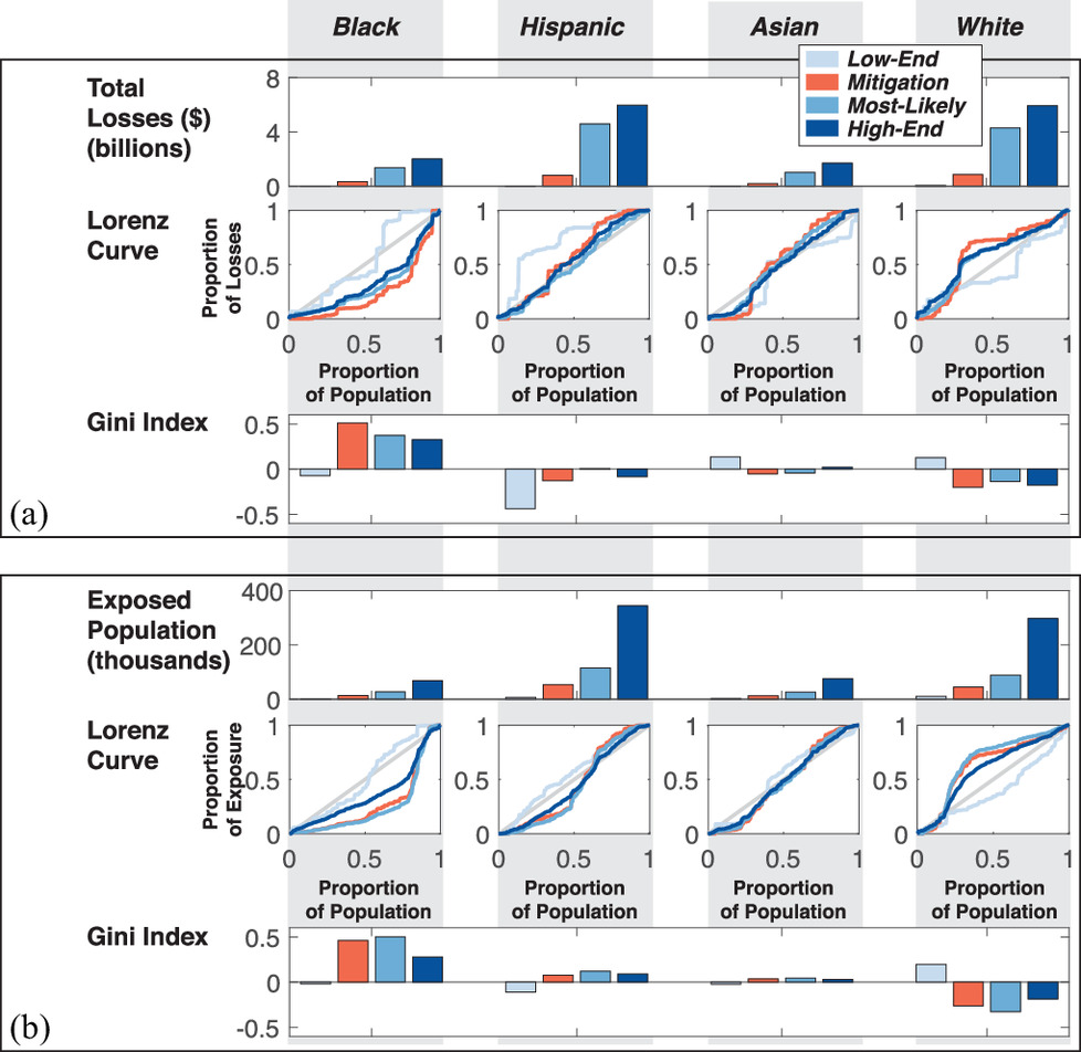
The strong and weak inequalities in damages and exposure for Black, White, and Hispanic populations noted above persist with increases in flood severity to the high-end scenario, but there are substantial changes to inequalities with decreases in flood severity to the low-end scenario. The strong inequalities in damages and exposure facing Black populations under the most-likely scenario are eliminated with the low-end scenario ( and ), the weak underexposure of White populations to flood damage with the most-likely scenario () reverses to a weak overexposure () with the low-end scenario, and the strong underexposure of White populations to flooding under the most-likely scenario () reverses to become a strong overexposure () with the low-end scenario. Finally, a strong underexposure to flood damage develops for Hispanic populations under the low-end scenario (). Recent research by Selsor et al. (2023) has also emphasized the sensitivity of flood exposure inequalities to flood magnitude.
Now attention turns to the mitigation scenario, which captures the change in flood hazards from raising levees by 1 m. Qualitatively based on Fig. 6, the effect of mitigation is similar to the effect of smaller flood peaks in that both reduce the areas exposed. Moreover, Fig. 7 depicts that the mitigation scenario leads to substantial reductions in total losses [Fig. 7(a)] and exposed populations [Fig. 7(b)] across all social groups, similar to the effect of smaller flood peaks. However, these results show that the mitigation scenario maintains strong inequalities in both flood damages () and flood exposure () for Black populations, and strong negative inequalities in both flood damages () and flood exposure () for White populations. This is attributed to the concentration of flood exposure near Carson (Fig. 6) where the Black population fraction is relatively high [Fig. 5(a)].
Comparing the Gini Index to Flood Exposure Representativeness
Inequalities in flood risk have previously been examined with other indicators such as risk ratios (Debbage 2019) and FER (Messager et al. 2021). The Gini index for flood exposure differs based on the consideration of the relative magnitude of flood depth, whereas risk ratios and FER use a binary classification: inside or outside of a flood zone. Moreover, risk ratios and FER require a depth tolerance to establish the edge of the flood zone, with smaller tolerances resulting in a larger flood zone that changes estimates of inequalities. To offer insight into uncertainties stemming from different methods, Fig. 8 presents a plot of FER versus the Gini index across the four social groups and the four scenarios considered in this study, with use of a 30 cm depth tolerance for FER. Note that FER values of unity correspond to equality, whereas a value of zero corresponds to equality using the Gini index. Nevertheless, Fig. 8 suggests that both FER and the Gini index identify a strong inequality in exposure for Black populations under the high-end, most-likely, and mitigation scenarios. However, the Gini index and FER send mixed signals about inequalities in exposure across social groups under low-end scenarios. For example, the Gini index points to equitable exposure for Black populations under the low-end scenario, while FER points to substantial underexposure (). Use of a smaller depth tolerance (10 cm) results in modest changes to FER estimates. For example, FER is 1.48 for Black residents under the most-likely scenario when the depth tolerance is 30 cm, while it is reduced to 1.23 when the depth tolerance is 3 cm. For White residents, FER is 0.85 under the most-likely scenario when the depth tolerance is 30 cm, while it is increased to 0.93 when the depth tolerance is 3 cm.

Integrating Social Inequality Data into Decision-Making Processes
Examining the impact of raising levees on flood exposure in Los Angeles shows overall benefits for all social groups with reduced exposure to the most-likely 1%-annual-chance hazard, but only minimal targeting to rectify inequalities in exposure across social groups. Conversely, these results show that lowering the peak flow holds greater promise for reducing both flood impacts (damages and exposed populations) and inequalities in impacts. In general, interventions can be expected to reshape exposure and inequalities in different ways, highlighting the need for and importance of inclusive processes of decision-making and an equity lens.
Inequality can be linked to inequity in many ways, and importantly, there is no single best approach. As a result, social inequality data computed at relevant scales (e.g., across states, counties, municipalities) can inform decision-making related to multiple aspects of equity and justice, recognizing that associated decision-making is inherently value-laden (Siders 2022). First, it can be used to inform the provision of resources for flood risk reduction, emergency management, relief, and recovery. Second, it can be used to evaluate the implications of interventions that cause both harms and benefits, such as home buyout programs (Mach and Siders 2021). Third, it can be used to incorporate uncertainty about such harms and benefits into decision-making, for example, under the deeper uncertainties of how sea level rise may shift flood exposure into the future (Marchau et al. 2019). Fourth, it can be used to prioritize participants within participatory processes, inform discussions, and support evaluation of experiences and outcomes, for instance, by identifying individuals and neighborhoods who may be disproportionately exposed yet less powerful within current flood management processes (Shi 2021). Fifth, it can be used to explicitly address and ameliorate historic and ongoing injustices, for example, those arising from racial stratification and differences in investments that have been made across communities (Bullard and Wright 2012).
Appropriate uses of exposure inequality data will depend on the priorities and goals of any given decision-making context, and a wide range of decision-making contexts are relevant. For example, there has long been recognition that flood hazard mitigation and risk management differentially benefit communities. Locations that are more rural or lower wealth, with greater presence of minoritized groups, are often less likely to receive flood infrastructure or recovery investments (Bullard and Wright 2012; Mach et al. 2019; Siders and Keenan 2020; Glavovic et al. 2022; Shi et al. 2021). Increasingly in the United States, federal agencies such as the Federal Emergency Management Agency or the U.S. Army Corps of Engineers are tracking and measuring the recipients of benefits (versus harms) from programs, grants, and projects. Exposure inequality data can shed light on the distribution of benefits across social groups, as well as inform efforts to increase equity, such as in the provision of support for hazard mitigation grant preparation or administration by local governments. Because flood risk reduction involves coordination across levels and agencies of government, the private sector, and civil society, measures of inequality are particularly important, as differences in who is experiencing harms versus benefits can be missed in aggregated indicators of outcomes.
New methods to quantify exposure and social inequalities for proposed projects and “no action” alternatives, as described herein, are responsive to recent state and federal policy in the U.S. to comprehensively consider economic, environmental, and social benefits in water resources project planning. At the federal level, the economic benefits of mitigation projects (e.g., reduced damages and emergency expenses) relative to costs (e.g., construction, operation, and maintenance) have historically served as the primary consideration for financial assistance. In particular, assistance from the Federal Emergency Management Agency (FEMA) has required a minimum of a 1:1 benefit/cost ratio in accordance with the Stafford Act (Miller et al. 2023), and assistance from the U.S. Army Corps of Engineers (Corps) has historically called for at least a 2.5:1 benefit/cost ratio (Fennell 2019). Broader social and environmental factors have only been considered after projects clear these monetary benefit thresholds (Fennell 2019). However, as of 2021, Corps policy has shifted in response to “concerns about an overreliance on national economic benefits as a required decision metric with secondary consideration of other important benefit categories” (James 2021). New Corps policy calls for applicants to “analyze benefits in total and equally across a full array of benefit categories” (James 2021).
A systematic approach to quantify social exposure and inequalities, as described here, would fit well within flood assistance programs in California, such as those made possible by state bond measures (California Department of Water Resources 2021). These programs direct applicants to document preliminary estimates of flood depth, flood extent, and flood risk reductions for proposed projects, and given that hydrologic and hydraulic modeling studies are usually completed to support this requirement, it would be straightforward for future programs to: (1) request estimates of exposed populations and exposure inequality by social groups as demonstrated herein, and (2) update the scoring of projects to reward project designs that demonstrate social equity.
Summary and Conclusions
Understanding how flood risks are distributed across populations and by social groups is important for developing equitable flood response measures and programs. Herein we demonstrate how a Lorenz curve and Gini index can be used to measure social inequalities in flood damage and flood exposure, that is, the concentration of flood risk by social groups. We describe the structuring of population, hazard (i.e., flood depth), damage, and social data (e.g., racial and ethnic fractions) required for exposure and inequality analysis, and a method of analysis. Whereas inequality of flood damages are described by a conventional Lorenz curve whereby cumulative losses are plotted versus cumulative population, inequality in flood exposure follows from a Lorenz curve where cumulative population-weighted flood depth is plotted versus cumulative population. Moreover, we show that spatial variations in population density have differing effects on inequalities in damages versus exposure as a consequence of population-weighting. In particular, increases in population density increase flood exposure but decrease the per person costs of flood damages.
An application of the Lorenz curve and Gini index method to Los Angeles County illustrates measurement of both flood damage and flood exposure inequalities at scale, and the examination of sensitivities to flood severity and flood infrastructure capacity. For example, under a most-likely 1%-annual-chance flood hazard, building damages and flood exposure disproportionately fall across Black populations, and these inequalities persist with a much higher flood peak (high-end scenario), and with greater infrastructure capacity (mitigation scenario), but are reduced with a much lower flood peak (low-end scenario). Additionally, the results show that flood risk inequalities for building damage and flood exposure may be slightly or even substantially different due to the spatial complexity of population density, flood hazard depth, and expected damages. These findings point to the importance of stakeholder dialogue and deliberations with an equity lens to more fully characterize the costs, benefits, and cobenefits of flood response options and develop adaptive pathways that are equitable and cost-effective.
Across the U.S., considering the social justice of public investments to manage environmental risks is of growing importance, and opportunities to inform investment decisions with social justice considerations are increasing. In particular, state and federal flood assistance programs offer greater flexibility to consider social factors in the evaluation and prioritization of resources. To this end, standardized quantitative metrics of the social dimensions of flood risk, as described herein, are increasingly important.
Data Availability Statement
An illustrative code for Lorenz curves and the Gini index is available at https://github.com/bfsand100/floodriskgini. A parcel-level database for Los Angeles County and codes for exposure inequality analysis are available through the Zenodo digital repository accessible at https://doi.org/10.7280/D1RH7Z.
Acknowledgments
The authors acknowledge assistance from M. Mierzwa for information about flood assistance programs in California, and S. Koller and W. Veatch for information about federal assistance policy and programs. The authors acknowledge the financial support of the NOAA Effects of Sea Level Rise Program Award No. NA23NOS4780283, and National Science Foundation support including Award Nos. CMMI-2031535, CMMI-2034308, and SCC-2305476.
Author contributions: The project concept was conceived by B.F.S. The Lorenz curve formulation for flood risk was developed B.F.S, S.J.D., and D.B., PRIMo modeling was completed by J.E.S., and damage modeling was completed by E.M.H. The narrative was prepared by B.F.S., K.J.M, D.B., E.M.H., and S.J.D. All authors contributed to review and editing.
References
Andreadis, K. M., O. E. Wing, E. Colven, C. J. Gleason, P. D. Bates, and C. M. Brown. 2022. “Urbanizing the floodplain: Global changes of imperviousness in flood-prone areas.” Environ. Res. Lett. 17 (10): 104024. https://doi.org/10.1088/1748-9326/ac9197.
Barry, J. M. 1997. The great Mississippi flood of 1927 and how it changed America. New York: Simon & Schuster.
Bates, P. 2023. “Uneven burden of urban flooding.” Nat. Sustainability 6 (1): 9–10. https://doi.org/10.1038/s41893-022-01000-9.
Bates, P. D., et al. 2021. “Combined modeling of us fluvial, pluvial, and coastal flood hazard under current and future climates.” Water Resour. Res. 57 (2): e2020WR028673. https://doi.org/10.1029/2020WR028673.
Billings, S. B., E. A. Gallagher, and L. Ricketts. 2022. “Let the rich be flooded: The distribution of financial aid and distress after hurricane harvey.” J. Financ. Econ. 146 (2): 797–819. https://doi.org/10.1016/j.jfineco.2021.11.006.
Bin, O., J. A. Bishop, and C. Kousky. 2012. “Redistributional effects of the national flood insurance program.” Public Finance Rev. 40 (3): 360–380. https://doi.org/10.1177/1091142111432448.
Brady, D., A. Blome, and H. Kleider. 2016. “How politics and institutions shape poverty and inequality.” In The Oxford handbook of the social science of poverty. New York: Oxford University Press.
Brady, D., and A. Bostic. 2015. “Paradoxes of social policy: Welfare transfers, relative poverty, and redistribution preferences.” Am. Sociol. Rev. 80 (2): 268–298. https://doi.org/10.1177/0003122415573049.
Brody, S. D., S. Zahran, P. Maghelal, H. Grover, and W. E. Highfield. 2007. “The rising costs of floods: Examining the impact of planning and development decisions on property damage in Florida.” J. Am. Plann. Assoc. 73 (3): 330–345. https://doi.org/10.1080/01944360708977981.
Bullard, R. D., and B. Wright. 2012. The wrong complexion for protection: How the government response to disaster endangers African American communities. New York: University Press.
California Department of Water Resources. 2021. “Floodplain Management, Protection and Risk Awareness (FMPRA) Grant Program.” Accessed May 1, 2023. https://water.ca.gov/Work-With-Us/Grants-And-Loans/Flood-Management-Protection-Risk-Awareness-Program.
Chakraborty, J., T. W. Collins, M. C. Montgomery, and S. E. Grineski. 2014. “Social and spatial inequities in exposure to flood risk in Miami, Florida.” Nat. Hazard. Rev. 15 (3): 04014006. https://doi.org/10.1061/(ASCE)NH.1527-6996.0000140.
Ciullo, A., J. H. Kwakkel, K. M. De Bruijn, N. Doorn, and F. Klijn. 2020. “Efficient or fair? Operationalizing ethical principles in flood risk management: A case study on the Dutch-German rhine.” Risk Anal. 40 (9): 1844–1862. https://doi.org/10.1111/risa.v40.9.
Debbage, N. 2019. “Multiscalar spatial analysis of urban flood risk and environmental justice in the Charlanta Megaregion, USA.” Anthropocene 28: 100226. https://doi.org/10.1016/j.ancene.2019.100226.
Domingue, S. J., and C. T. Emrich. 2019. “Social vulnerability and procedural equity: Exploring the distribution of disaster aid across counties in the United States.” Am. Rev. Public Adm. 49 (8): 897–913. https://doi.org/10.1177/0275074019856122.
England, K., and K Knox. 2015. Targeting flood investment and policy to minimise flood disadvantage. York: Joseph Rowntree Foundation.
FEMA. 2018. “Guidance for flood risk analysis and mapping, flood depth and analysis grids.” Federal Emergency Management Agency. Accessed May 1, 2023. https://www.fema.gov/sites/default/files/2020-02/Flood_Depth_and_Analysis_Grids_Guidance_Feb_2018.pdf.
FEMA. 2022a. “FEMA factsheet: Flood assessment structure tool.” Federal Emergency Management Agency. Accessed May 1, 2023. https://www.fema.gov/sites/default/files/documents/fema_flood-assessment-structure-tool.pdf.
FEMA. 2022b. “Hazus flood technical manual, hazus 5.1.” Federal Emergency Management Agency. Accessed May 1, 2023. https://www.fema.gov/sites/default/files/documents/fema_hazus-flood-model-technical-manual-5-1.pdf.
Fennell, A.-M. 2019. Army corps of engineers. Evaluations of flood risk management projects could benefit from increased transparency. Rep. No. GAO-20-43. Washington, DC: US Government Accountability Office.
Glavovic, B., R. Dawson, W. Chow, M. Garschagen, M. Haasnoot, C. Singh, and A Thomas. 2022. “Cross-chapter paper 2: Cities and settlements by the sea.” In Climate Change 2022: Impacts, Adaptation and Vulnerability. Contribution of Working Group II to the Sixth Assessment Report of the Intergovernmental Panel on Climate Change, 2163–2194. Cambridge: Cambridge University Press.
Hino, M., S. Belanger, C. Field, A. Davies, and K. Mach. 2019. “High-tide flooding disrupts local economic activity.” Sci. Adv. 5 (2): eaau2736. https://doi.org/10.1126/sciadv.aau2736.
Hornbeck, R., and S. Naidu. 2014. “When the levee breaks: Black migration and economic development in the American South.” Am. Econ. Rev. 104 (3): 963–990. https://doi.org/10.1257/aer.104.3.963.
Howard, C., and R. Wilkes. 2022. “What is the difference between equity and equality?” Divided We Fall. Accessed May 1, 2023. https://dividedwefall.org/equity-vs-equality/.
James, R. D. 2021. “Policy directive – comprehensive documentation of benefits in decision document.” Washington, DC: Dept. of the Army, Memorandum for Commanding General, US Army Corps of Engineers.
Jones, L. 2019. The big ones: How natural disasters have shaped us (and what we can do about them). New York: Anchor.
Kahl, D. T., J. E. Schubert, A. Jong-Levinger, and B. F. Sanders. 2022. “Grid edge classification method to enhance levee resolution in dual-grid flood inundation models.” Adv. Water Resour. 168: 104287. https://doi.org/10.1016/j.advwatres.2022.104287.
Kakwani, N. C. 1977. “Measurement of tax progressivity: An international comparison.” Econ. J. 87 (345): 71–80. https://doi.org/10.2307/2231833.
Kousky, C. 2015. “A historical examination of the corps of engineers and natural valley storage protection: The economics and politics of ‘green’ flood control.” J. Nat. Resour. Policy Res. 7 (1): 23–40. https://doi.org/10.1080/19390459.2014.963372.
Lindersson, S., E. Raffetti, M. Rusca, L. Brandimarte, J. Mård, and G. Di Baldassarre. 2023. “The wider the gap between rich and poor the higher the flood mortality.” Nat. Sustainability 6 (8): 995–1005. https://doi.org/10.1038/s41893-023-01107-7.
Lorenz, M. O. 1905. “Methods of measuring the concentration of wealth.” Publ. Am. Stat. Assoc. 9 (70): 209–219.
Los Angeles County. 2022. “Assessor Parcels Data 2006 thru 2021.” Los Angeles County. Accessed February 19, 2023. https://data.lacounty.gov/datasets/assessor-parcels-data-2006-thru-2021/.
Maantay, J., and A. Maroko. 2009. “Mapping urban risk: Flood hazards, race, and environmental justice in New York.” Appl. Geogr. 29 (1): 111–124. https://doi.org/10.1016/j.apgeog.2008.08.002.
Mach, K. J., M. Hino, A. Siders, S. F. Koller, C. M. Kraan, J. Niemann, and B. F. Sanders. 2022. “From flood control to flood adaptation.” Oxford Research Encyclopedia of Environmental Science. Accessed May 1, 2023. https://doi.org/10.1093/acrefore/9780199389414.013.819.
Mach, K. J., C. M. Kraan, M. Hino, A. Siders, E. M. Johnston, and C. B. Field. 2019. “Managed retreat through voluntary buyouts of flood-prone properties.” Sci. Adv. 5 (10): eaax8995. https://doi.org/10.1126/sciadv.aax8995.
Mach, K. J., and A. Siders. 2021. “Reframing strategic, managed retreat for transformative climate adaptation.” Science 372 (6548): 1294–1299. https://doi.org/10.1126/science.abh1894.
Marchau, V. A., W. E. Walker, P. J. Bloemen, and S. W Popper. 2019. Decision making under deep uncertainty: From theory to practice. Berlin: Springer Nature.
Messager, M. L., A. K. Ettinger, M. Murphy-Williams, and P. S. Levin. 2021. “Fine-scale assessment of inequities in inland flood vulnerability.” Appl. Geogr. 133: 102492. https://doi.org/10.1016/j.apgeog.2021.102492.
Miller, B. M., N. Clancy, D. C. Ligor, G. Kirkwood, D. Metz, S. Koller, and S. Stewart. 2023. The cost of cost-effectiveness. Expanding equity in federal emergency management agency hazard mitigation assistance grants. Rep. No. Homeland Security Operational Analysis Center operated by the RAND Corporation. Accessed May 1, 2023. https://www.rand.org/pubs/research_reports/RRA2171-1.html.
Milly, P. C., J. Betancourt, M. Falkenmark, R. M. Hirsch, Z. W. Kundzewicz, D. P. Lettenmaier, and R. J. Stouffer. 2008. “Stationarity is dead: Whither water management?.” Science 319 (5863): 573–574. https://doi.org/10.1126/science.1151915.
Molinaroli, E., S. Guerzoni, and D. Suman. 2019. “Do the adaptations of venice and miami to sea level rise offer lessons for other vulnerable coastal cities?” Environ. Manage. 64 (4): 391–415. https://doi.org/10.1007/s00267-019-01198-z.
Montz, B., and E. C. Gruntfest. 1986. “Changes in American urban floodplain occupancy since 1958: The experiences of nine cities.” Appl. Geogr. 6 (4): 325–338. https://doi.org/10.1016/0143-6228(86)90034-2.
Orsi, J. 2004. Hazardous metropolis: Flooding and urban ecology in Los Angeles. Berkeley, CA: Univ. of California Press.
Sanders, B. F., and S. B. Grant. 2020. “Re-envisioning stormwater infrastructure for ultrahazardous flooding.” Wiley Interdiscip. Rev.: Water 7 (2): e1414. https://doi.org/10.1002/wat2.v7.2.
Sanders, B. F., and J. E. Schubert. 2019. “Primo: Parallel raster inundation model.” Adv. Water Resour. 126: 79–95. https://doi.org/10.1016/j.advwatres.2019.02.007.
Sanders, B. F., J. E. Schubert, D. T. Kahl, K. J. Mach, D. Brady, A. AghaKouchak, F. Forman, R. A. Matthew, N. Ulibarri, and S. J. Davis. 2023. “Large and inequitable flood risks in Los Angeles, California.” Nat. Sustainability 6 (1): 47–57. https://doi.org/10.1038/s41893-022-00977-7.
Sanderson, D., and D. Cox. 2023. “Comparison of national and local building inventories for damage and loss modeling of seismic and tsunami hazards: From parcel-to city-scale.” Int. J. Disaster Risk Reduct. 93: 103755. https://doi.org/10.1016/j.ijdrr.2023.103755.
Schroder, K., M. A. Hummel, K. M. Befus, and P. L. Barnard. 2022. “An integrated approach for physical, economic, and demographic evaluation of coastal flood hazard adaptation in Santa Monica Bay, California.” Front. Mar. Sci. 9: 1052373. https://doi.org/10.3389/fmars.2022.1052373.
Schubert, J. E., A. Luke, A. AghaKouchak, and B. F. Sanders. 2022. “A framework for mechanistic flood inundation forecasting at the metropolitan scale.” Water Resour. Res. 58 (10): e2021WR031279. https://doi.org/10.1029/2021WR031279.
Selsor, H., B. P. Bledsoe, and R. Lammers. 2023. “Recognizing flood exposure inequities across flood frequencies.” Anthropocene 42: 100371. https://doi.org/10.1016/j.ancene.2023.100371.
Shi, L. 2021. “From progressive cities to resilient cities: Lessons from history for new debates in equitable adaptation to climate change.” Urban Aff. Rev. 57 (5): 1442–1479. https://doi.org/10.1177/1078087419910827.
Shi, L., S. Ahmad, P. Shukla, and S. Yupho. 2021. “Shared injustice, splintered solidarity: Water governance across urban-rural divides.” Global Environ. Change 70: 102354. https://doi.org/10.1016/j.gloenvcha.2021.102354.
Siders, A. 2022. “The administrator’s dilemma: Closing the gap between climate adaptation justice in theory and practice.” Environ. Sci. Policy 137: 280–289. https://doi.org/10.1016/j.envsci.2022.08.022.
Siders, A., and J. M. Keenan. 2020. “Variables shaping coastal adaptation decisions to armor, nourish, and retreat in North Carolina.” Ocean Coastal Manage. 183: 105023. https://doi.org/10.1016/j.ocecoaman.2019.105023.
Smiley, K. T. 2020. “Social inequalities in flooding inside and outside of floodplains during hurricane harvey.” Environ. Res. Lett. 15 (9): 0940b3. https://doi.org/10.1088/1748-9326/aba0fe.
Tate, E., M. A. Rahman, C. T. Emrich, and C. C. Sampson. 2021. “Flood exposure and social vulnerability in the United States.” Nat. Hazard. 106 (1): 435–457. https://doi.org/10.1007/s11069-020-04470-2.
Tate, E., A. Strong, T. Kraus, and H. Xiong. 2016. “Flood recovery and property acquisition in Cedar Rapids, Iowa.” Nat. Hazard. 80 (3): 2055–2079. https://doi.org/10.1007/s11069-015-2060-8.
Ulibarri, N., C. Valencia-Uribe, B. F. Sanders, J. Schubert, R. Matthew, F. Forman, M. Allaire, and D. Brady. 2023. “Framing the problem of flood risk and flood management in Metropolitan Los Angeles.” Weather Clim. Soc. 15 (1): 45–58. https://doi.org/10.1175/WCAS-D-22-0013.1.
US Census Bureau. 2020a. “2020 Census, Los Angeles County, California.” US Census. Accessed January 30, 2023. https://www.census.gov/data.html.
US Census Bureau. 2020b. “American Community Survey.” US Census. Accessed January 31, 2023. https://www.census.gov/programs-surveys/acs.
US Census Bureau. 2022. “Glossary.” US Census. Accessed April 11, 2022. https://www.census.gov/programs-surveys/geography/about/glossary.html.
USACE. 2022. “National Structure Inventory.” US Army Corps of Engineers. Accessed May 1, 2023. https://www.hec.usace.army.mil/confluence/nsi.
Vahedifard, F., M. Azhar, and D. C. Brown. 2023. “Overrepresentation of historically underserved and socially vulnerable communities behind levees in the United States.” Earth’s Future 11 (9): e2023EF003619. https://doi.org/10.1029/2023EF003619.
Wing, O. E., P. D. Bates, C. C. Sampson, A. M. Smith, K. A. Johnson, and T. A. Erickson. 2017. “Validation of a 30 m resolution flood hazard model of the conterminous united states.” Water Resour. Res. 53 (9): 7968–7986. https://doi.org/10.1002/wrcr.v53.9.
Wing, O. E., P. D. Bates, A. M. Smith, C. C. Sampson, K. A. Johnson, J. Fargione, and P. Morefield. 2018. “Estimates of present and future flood risk in the conterminous United States.” Environ. Res. Lett. 13 (3): 034023. https://doi.org/10.1088/1748-9326/aaac65.
Wing, O. E., W. Lehman, P. D. Bates, C. C. Sampson, N. Quinn, A. M. Smith, J. C. Neal, J. R. Porter, and C. Kousky. 2022. “Inequitable patterns of us flood risk in the anthropocene.” Nat. Clim. Change 12 (2): 156–162. https://doi.org/10.1038/s41558-021-01265-6.
Wing, O. E., N. Pinter, P. D. Bates, and C. Kousky. 2020. “New insights into US flood vulnerability revealed from flood insurance big data.” Nat. Commun. 11 (1): 1444. https://doi.org/10.1038/s41467-020-15264-2.
Information & Authors
Information
Published In

ASCE OPEN: Multidisciplinary Journal of Civil Engineering
Volume 2 • Issue 1 • April 2024
Copyright
This work is made available under the terms of the Creative Commons Attribution 4.0 International license, https://creativecommons.org/licenses/by/4.0/.
History
Received: Jun 9, 2023
Accepted: Jan 3, 2024
Published online: Apr 15, 2024
Published in print: Apr 15, 2024
Discussion open until: Sep 15, 2024
Authors
Metrics & Citations
Metrics
Citations
Download citation
If you have the appropriate software installed, you can download article citation data to the citation manager of your choice. Simply select your manager software from the list below and click Download.