A Generic Deep Learning–Based Computing Algorithm in Support of the Development of Instrumented Bikes
Publication: ASCE OPEN: Multidisciplinary Journal of Civil Engineering
Volume 2, Issue 1
Abstract
The paper introduces a generic deep learning–based method using a sliding window computing algorithm based on long short-term memory (LSTM) networks for the classification of potential anomalies (e.g., cracks, potholes, bumps, and uneven surfaces) in support of the development of an instrumented bike. The instrumented bike provides a real-time platform to sense, store, transmit, and analyze cycling information through a sensor logger, smartphone, and the proposed LSTM-based sliding window computing algorithm. The paper is to address concerns with respect to existing factors such as weight of cyclists, speeds, types of bikes, and threshold setting that have an impact on the accuracy of identification of potential anomalies during instrumented cycling activities. The LSTM-based sliding window computing algorithm is designed in a way that it analyzes and localizes anomalies without any human-controlled supervision (threshold setting) while achieving human-level perception. Two bike routes were selected to validate the effectiveness of the sliding window computing algorithm in the identification of anomalies involving four cyclists. Based on the computing results from the two field tests, the numbers of distressed pavement areas from the four cyclists were 53, 51, 46, and 48, respectively. The follow-up p-value of ANOVA test result is 0.98, indicating the difference in detected anomalies among the four cyclists is not significant. Therefore, the paper concludes that the LSTM-based sliding window computing algorithm has the ability to effectively detect anomalies of cycling trails and it also provides an effective and efficient technique to replace the human-made threshold setting in support of the development of instrumented bikes and promote cycling as a daily mode of transportation.
Introduction
The market for connected vehicles has been growing dramatically in recent years, with the global market expected to reach $225.16 billion by 2027 (AMR 2021). However, as a part of intelligent transportation systems, the use of geospatial and remote sensing in cycling mobility has yet to receive significant attention, likely due to limited efforts in manufacturing instrumented bikes or smart bikes to promote cycling mobility and reduce greenhouse gas emissions. Particularly, during crises such as the coronavirus disease 2019 (COVID-19) pandemic, an activity like cycling can decrease exposure to others on public transport, reduce air pollution, and promote improved health and well-being. When cycling on bike facilities, the roadway surface structure plays an important role in bike ride quality; pavement surfaces with anomalies (i.e., potholes, uneven surface, cracks, bumps, etc.) could reduce the quality of bike trails, increase the risk of accidents, and decrease the cycling safety. With the continued growth in cycling activity and infrastructure throughout the United States, the question of how to obtain real-time information on cycling facilities that would help better maintain the quality of these facilities and provide a safe environment for cyclists has become a concern among city, county, and state engineers. The use of sensors/accelerometers attached to bikes has been investigated by numerous researchers to study cyclist behavior, monitor cycling motion, and measure the force of pedaling (ECF 2021a, b; Leitner et al. 2014; Liu et al. 2015; Pedotti et al. 2016; Pigatto et al. 2016). However, this technology presents an untapped potential to assess cycling facility surface conditions. There is an urgent need to meet increasing demands for cyclist safety to motivate increased activity. Hence, it is believed that the interactive behavior of cyclists plays an important role in bringing together improved bike mobility and community engagement. An instrument bike has been developed by Ho et al. (2021, 2019) and Qiu et al. (2018). The instrumented bike is equipped with a sensor logger and a mobile application, and it aims at providing a tool that can be taken into account for detecting anomalies on bike trails/routes as well as sharing real-time information with cyclists around them. However, the previously developed threshold setting used to identify potential anomalies has raised concerns that need to be addressed. For example, some argue that existing factors such as the weight of cyclists, speeds, tire pressures, types of bikes, and threshold setting have an impact on the accuracy of identification of potential anomalies during cycling activities. In the past, threshold values to detect anomalies needed to be adjusted in the data analysis process to obtain better prediction results. However, based on our experience, this human-made setting is time-consuming and inefficient for anomaly detection. To address the issues, this paper is presented to develop an advanced computing method using a generic deep learning–based computing algorithm to: (1) replace the current human-made threshold setting; and (2) provide a better and more accurate computing method for anomaly identification on bike trails/routes.
The structure of the paper is arranged using the following flowchart (Fig. 1).

Development of Computing Algorithm: A Generic Deep Learning Approach
This section presents a methodology using a deep learning computing algorithm to process, analyze, and detect anomalies on bike trails/routes.
Literature Review and Motivation
The instrumented bike (Ho et al. 2019, 2021; Qiu et al. 2018) provides a reliable framework to sense, transmit, and store acceleration information on various bike routes. The variation of acceleration in three-axes can physically encode the intrinsic features of anomalies (e.g., cracks and potholes): the acceleration will change dramatically in either axis when cracks/potholes are encountered. However, taking advantage of those collected acceleration data to detect and localize anomalies becomes inherently intractable. Previously, the window-interpolation method proposed by Qiu et al. (2018) was used to detect anomalies by dividing the data into many nonoverlapping chunks and then determining the difference between maximum and minimum accelerations within one window. However, as previously mentioned, the handcrafted threshold varies dramatically in different scenarios. Even though different thresholds can be tested out in different scenarios, it is practically infeasible to handcraft thresholds in every single event. This method even fails in some cases where: (1) two adjacent anomalies are very close; (2) the anomalies are very small; and (3) the speed is so fast that it is beyond the sampling frequency. This is because this method only works for a limited sampling frequency (around 50 Hz), while the accelerometer is capable of a higher sampling frequency (around 200 Hz), resulting in the sparsity of samples within a given time slot.
Recently, the advances in many machine learning techniques have enabled us to take advantage of the huge amount of data to uncover the hidden pattern within a sequence of acceleration data. The majority of them (Lu et al. 2014; Zhao et al. 2018; Pienaar and Malekian 2019; Hammerla et al. 2016; Abbaspour et al. 2020) however need annotated data to train a classifier in a supervised setting to identify whether a subsequence of the acceleration data contains anomalies. In practice, it is laborious to manually label the anomaly patterns within a sequence of acceleration data. In addition, human bias may also be introduced during labeling, as manual annotation is equivalent to perceptually identifying the anomalies. Furthermore, many classical powerful machine learning methods (e.g., support vector machine, random forest) still need to handcraft features and generally fail to capture the long-range time dependencies between data points. Anomalies are jointly encoded by a small subsequence of acceleration in a specific order within a certain time slot. For example, the acceleration in the Z-axis first goes up and then goes down for any anomalies or vice versa. Therefore, a generic method is desired to detect and localize anomalies while minimizing the impact of variations in physical conditions such as speeds, sampling frequency, weather, and different bikes. Recently, recurrent neural networks (RNNs)-based methods have been widely used to process acceleration data in human activity recognition tasks (Zhao et al. 2018; Pienaar and Malekian 2019; Hammerla et al. 2016; Abbaspour et al. 2020). The RNNs have the capability of capturing the dependencies of data concerning time, which represents the acceleration data in a probabilistic way over time. However, the RNN-based methods are trained in a supervised way (Zhao et al. 2018; Pienaar and Malekian 2019; Hammerla et al. 2016; Abbaspour et al. 2020) that inputs an acceleration sequence and outputs a label indicating the classification category (e.g., cracks or noncracks). However, the process of annotating acceleration data is time-consuming and inefficient. To tackle the lack of annotated data, the team built on the concept of another family of machine learning techniques—unsupervised representation learning (Malhotra et al. 2016). The idea is that instead of learning the direct mapping from acceleration sequence to anomaly label, the algorithm learns the representation of normal bike routes on anomaly-free areas. The whole idea was implemented as an RNN-based autoencoder neural network (Srivastava et al. 2015; Bengio et al. 2013). During inference, the anomalies can be detected as their patterns are different from those from anomaly-free regions. Conversely, when several cyclists travel on the same bike trails, regardless of their speeds and bikes, all patterns and signals from anomaly regions will be registered and recorded for analysis. In this regard, the team takes advantage of the sliding window technique associated with long short-term memory (LSTM) architecture to localize anomalies (i.e., cracks/potholes) to map them to corresponding location coordinates.
Table 1 summarizes the results of all literature reviews regarding the types of research conducted, the number of sensors used, research purposes, and their results.
| Author (year) | Type of research | Sensors used | Research purpose | Results |
|---|---|---|---|---|
| Abbaspour et al. (2020) | Comparative analysis of hybrid deep learning models | Wearable sensors (gyroscopes, accelerometers, IMU sensors), ambient sensors (cameras, GPSs, PIRs), smartphone sensors | Investigate the effectiveness of CNNs integrated with RNNs in recognizing human activities | The study applied four hybrid deep learning models for human activity recognition (HAR), integrating CNNs with various RNNs. The results showed high accuracy, surpassing that of individual CNNs or RNNs. |
| Bengio et al. (2013) | Theoretical review on representation learning | Not applicable | Review recent work in unsupervised feature learning and deep learning | The study explored contractive autoencoders in representation of learning, showing the effectiveness in estimating tangent vectors to high-density manifolds, and allowing for the demonstration of plausible additive deformations of inputs. |
| Hammerla et al. (2016) | Empirical study on HAR using wearables | Wearable sensors (accelerometers, IMUs) | Explore deep learning approaches for HAR | The authors explored the performance of state-of-the-art deep learning approaches for HAR 1538 using wearable sensors. The paper also indicated that DNNs are very sensitive to their hyperparameters and require a significant investment into parameter exploration. |
| Lu et al. (2014) | Review on connected vehicle technologies | Various sensors in connected vehicles | Review CV technologies, challenges, and opportunities | The authors highlighted the challenge of obtaining accurately labeled data that has an impact on the effective training of machine learning models to identify irregularities in vehicle behaviors. The research underscored the dependency on high-quality, annotated data sets for developing robust and reliable anomaly-detection systems in the context of vehicle connectivity. The paper suggested a future direction toward enhancing data annotation methods and exploring more sophisticated machine learning techniques that can adapt to the complexities of acceleration data, thereby improving the accuracy and efficiency of anomaly detection. |
| Pienaar and Malekian (2019) | Empirical study on HAR using LSTM-RNN | Raw sensor data from WISDM data set | Model and train LSTM-RNN for HAR | Bidirectional LSTMs were found to outperform the current state-of-the-art models on the data set. In addition, RNNs excelled in activities with a natural order and shorter duration, whereas CNNs were recommended for prolonged, repetitive activities like walking or running. Moreover, while regular DNNs require extensive parameter exploration, more sophisticated models like CNNs and RNNs could show a smaller spread in performance, suggesting ease in finding effective configurations. |
| Srivastava et al. (2015) | Unsupervised learning of video representations using LSTMs | Video sequences | Explore LSTM networks to learn video representations | The study involved training models on data sets of moving Modified National Institute of Standards and Technology (MNIST) digits and natural image patches to learn video representations in an unsupervised manner using LSTM-based models. The author improved classification accuracy, especially with few training examples. The experiments showcased the LSTM’s ability to learn meaningful representations from video sequences and improved predictions in action recognition tasks. |
| Zhao et al. (2018) | Applied Research in Deep Learning for HAR | Accelerometers, gyroscopes, etc. | To propose a deep network architecture using residual bidirectional LSTM to address HAR problems, aiming to improve recognition rates by capturing temporal dependencies and preventing gradient vanishing | The study introduced the Res-Bidir-LSTM framework for HAR, enhancing learning speed and accuracy through residual and bidirectional connections. Experiments showed a 4.8% accuracy improvement for the UCI data set and a 3.7% increase in F1 score for the opportunity data set. Key findings included the significance of window size (500‒5,000 ms) for optimal information processing and the necessity of tailoring network architecture and hyperparameters to data set complexity, with cell number adjustments based on feature and label richness. |
Note: CNNs = convolutional neural networks; CV = connected vehicles; DL = deep learning; DNN = deep neural network; GPSs = global positioning systems; HAR = human activity recognition; IMU = inertial measurement unit; LSTM = long short-term memory; LSTM-RNN = long short-term memory recurrent neural network; PIRs = passive infrared sensors; Res-Bidir-LSTM = deep residual bidirectional long short-term memory; RNNs = recurrent neural networks; and WISDM = wireless sensor data mining.
Thus, in this paper, the team presents an automated and systematic approach to detect and localize anomalies without human supervision. The whole framework is illustrated in Fig. 2. The objectives of the proposed computing method are as follows:
1.
Designing an LSTM-based autoencoder neural network to classify anomalies (i.e., cracks/potholes).
2.
Incorporating sliding windows with neural networks to localize anomalies (i.e., cracks/potholes) and output candidates.
3.
Efficient implementation for the combined sliding window technique and neural network inference (LSTM-based sliding window computing algorithm).
4.
Postprocessing strategies to aggregate the anomaly candidates.

Background of an Instrumented Bike
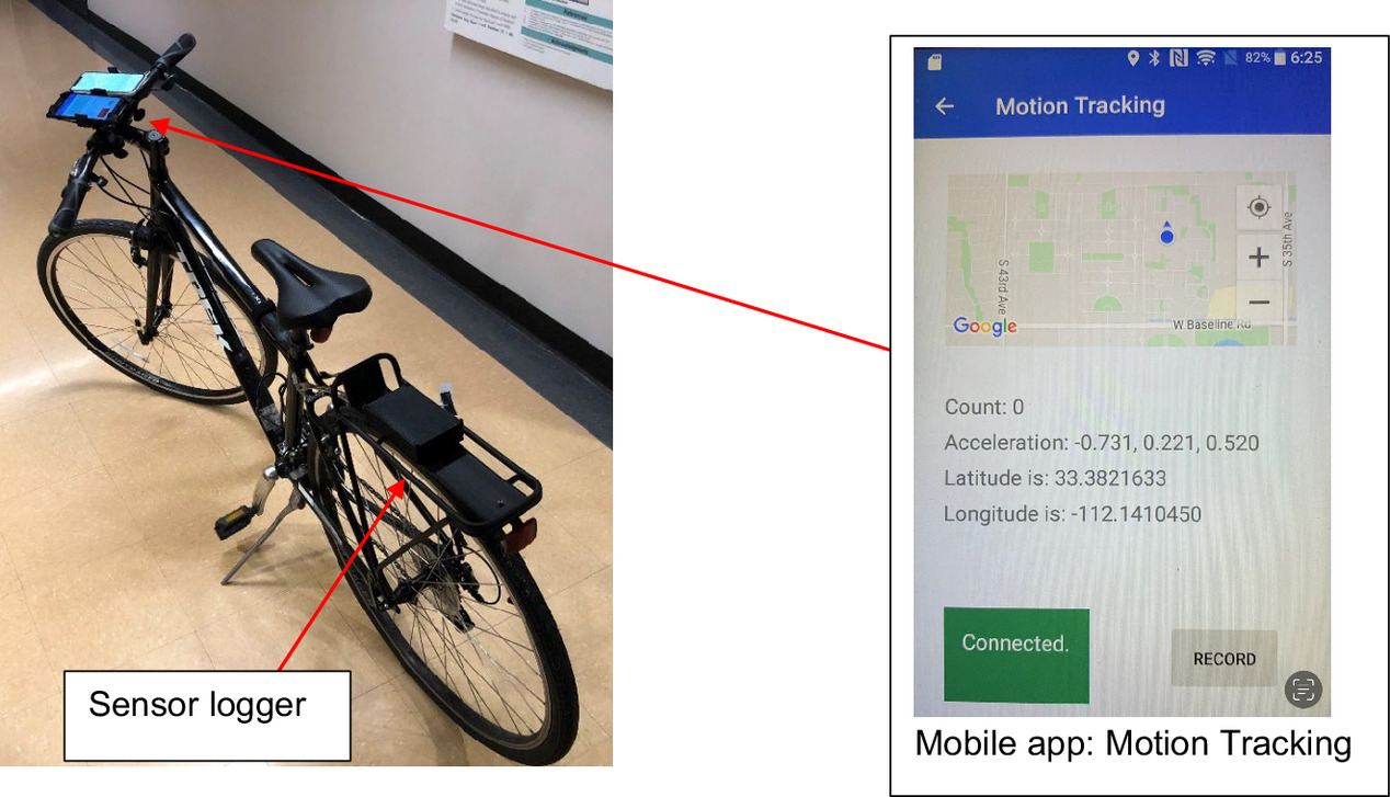
The technique of using accelerometers to monitor and track road conditions has been broadly used through a variety of applications in the vehicular and cycling communities. In early 2018, the team embarked on the development of an instrumented bike with a goal to detect potential anomalies (cracks, potholes, bumps, etc.) along bike routes. An instrumented bike is equipped with a sensor logger, a video device (e.g., GoPro), an inertial measurement unit (accelerometer and gyroscope), a global positioning system (GPS), a wireless network adapter (WIFI), a micro Secure Digital (microSD) card data storage, and a battery (Ho et al. 2021) as shown in Fig. 3. An instrumented bike mobile app named Motion Tracking developed by our team is installed in a smartphone paired with an instrumented bike. One of the advantages of using an instrumented bike is the ability to share real-time cycling information with cyclists nearby, allowing cyclists extra time to adjust their cycling routes to avoid any potential risk of accidents. This process is illustrated as follows: When a cyclist travels on a bike trail, the vibration data/signals will be registered by the sensor logger and then wirelessly transferred to the smartphone or stored in the sensor logger. The data will be retrieved from either a smartphone or a sensor logger, processed, and analyzed to determine if any potential anomalies (e.g., bumps, uneven surfaces, potholes, and cracks) are identified. Identified anomalies are recorded in a csv. format, georeferenced, and displayed in a map using geographic information systems (GIS) software (i.e., ArcGIS version 10) or the Motion Tracking app. Those cyclists who have downloaded the mobile app will be notified of anomaly locations prior to their cycling trip so that they can plan ahead to adjust cycling routes or ride cautiously to avoid any accidents. The previous implementation of the instrumented bike between 2019 and 2020 demonstrated that this is an effective method to facilitate the quality control of cycling facilities and promote cycling mobility (Ho et al. 2019, 2021; Qiu et al. 2018).
Based on the current practice, a threshold value of 0.95 g was used in the computing process to classify anomalies through instrumented cycling (Ho et al. 2019, 2021). However, this threshold is a human-made decision process based on data distributions and statistical analysis, and its setting is highly dependent on several factors such as different bikes (street bikes, mountain bikes, beach cruisers, etc.), cycling speeds, tire pressures, the weight of cyclists, and weather conditions of bike routes (wet or dry); these would have a significant impact on the accuracy of anomaly identification. To address this issue, the paper presents an advanced computing algorithm using a generic deep learning approach to improve the existing computing efficiency and accuracy in anomaly identification and advance the use of instrumented bikes.
Data Set and Preprocessing
The data set used in all the experiments and training was collected by Ho et al. (2019, 2021) and Qiu et al. (2018). The sensor developed in the paper is a nine-axis sensor incorporating a three-axis accelerometer, a three-axis gyroscope, and a three-axis magnetometer. It has an integrated 32-bit microcontroller unit while the accelerometer sensor has a maximum range of ± 16g and the gyroscope has a range of ± 2,000°/s, where each sample is of 16 bits. Prior to assembly of a sensor logger, all sensors were tested in the laboratory and calibrated based on the aforementioned range to ensure the accuracy of each sensor according to the research team’s design. The original data consist of accelerometer values in three axes (x, y, z) and corresponding location coordinates (longitude, latitude). Fourier transform process observes that the accelerations in all three axes change dramatically when encountering a crack/pothole, the magnitude of the acceleration in all directions was used as the input feature so that all the results can be better visualized in this paper (while the team leaves the possibility of using more features to enhance the robustness). The magnitude is computed as the following equation:where X, Y, Z = acceleration values in x-, y-, z-directions, respectively.
(1)
The magnitude is further standardized by subtracting its mean and dividing by the standard deviation as expressed in the following equation:where μ = mean; and σ = standard deviation, so that it has the same mean and deviation.
(2)
Note that standardization is a general preprocessing step in neural network training as it improves the numerical stability of the model and may boost the convergence.
The training and validation data sets were collected on three different bike routes at different times containing 3,000 samples. All data were resampled to overlapping windows with a size of seven as a data augmentation strategy. After data were standardized; fast Fourier transform (FFT) was performed to change the data to the frequency domain from the time domain.
Classification with LSTM Autoencoder
Anomaly detection from acceleration data is a challenging task for machines, even though the variation of accelerations in three axes can physically encode the pattern of anomalies. The patterns of an anomaly can be distinguished effortlessly by human-beings out of a sequence of accelerations. Human beings recognize anomalies by their visualization and cycling experience based on the dramatic changes of acceleration within a certain subsequence. Therefore, autoencoders that mimic human beings to learn the representation of anomalies without annotated data are desired for this task.
An autoencoder is made up of the encoder and the decoder. The encoder projects the input data space χ into the latent space Γ, which is also known as the latent representation, via a function φ:χ → Γ. The decoder, whose architecture generally mirrors that of the encoder, reconstructs the input data from the latent representation via a function: Γ → χ . Mathematically, an autoencoder is defined as follows:
(3)
Eq. (3) minimizes the distance between the input data and the output reconstruction from the network. The formulation of the autoencoder suggests that the training of an autoencoder is fully unsupervised, or technically self-supervised, which is another motivation for using the autoencoder architecture. However, anomalies are not commonplace during cycling, since extracting them from the original signal is equivalent to detecting them. Alternatively, the representation of anomaly-free cycling sequence (smoothing sequence), as they are more easily obtained, can be used to help recognize cracks/potholes as anomalies. Once the reconstruction loss in the inference is greater than the maximal validation reconstruction loss during training, the sequence is identified as an anomaly.
Another insight to perceptually recognize human-level anomalies is that the order of the data points supports human beings to identify them. For example, the acceleration in the Z-direction first goes up, then goes down, or vice versa. Therefore, the dependencies between the data points are another key factor to identify anomalies, leading to the criteria of RNNs. The RNNs capture the temporal dependencies (or orders) of sequence input by propagating the information from the current state to the next state. The vanilla RNNs, in practice, lose long-term dependencies (Bengio et al. 1994). Therefore, the team decided to replace the vanilla RNNs with LSTM architecture (Bayer 2015). The LSTM unit is incorporated into the autoencoder architecture so that the network can learn the sequence representation in a self-supervised way. The proposed network is implemented as an LSTM autoencoder as shown in Fig. 4. A follow-up training process is performed to evaluate the effectiveness of our methodology. A simple architecture including two LSTM units with two layers was used for both the encoder and the decoder, and the performance is considered satisfactory; the stationary training loss and validation loss are close to 0 as is shown in Fig. 5. Based on the training, the next step is to make the LSTM architecture more efficient to detect anomalies using a sliding window algorithm previously developed by the team.


In our proposed computing method, the team employed an autoencoder architecture based on LSTM networks, which are well suited for handling sequential data. The encoder consists of two LSTM layers with hidden dimensions of 128 and 64, respectively. These layers are responsible for mapping the input sequence (with length of N and dimensions of d) to a vector with a dimension of 64 in the latent space. The decoder component of our autoencoder is responsible for reconstructing the original input data from the latent representation. It consists of two LSTM layers followed by a linear layer. The first LSTM layer has a hidden dimension of 64, and the second LSTM layer has a hidden dimension of 128. After the LSTM layers, the team used a linear layer with an input size of 128 and an output size of 1 to transform the latent representation back into the original data space.
By self-supervised/unsupervised training on a data set (i.e., input is a sequence, and the target is the same sequence), the LSTM autoencoder learns the typical/regular/normal patterns and correlations within the data and the abnormal patterns will be automatically treated as noise by the network.
During the decoding phase, the network attempts to reconstruct the input data from the encoded representation from the latent space. Since the autoencoder only learns to reconstruct normal data well, if the input data contain anomalies, the reconstruction will be poor, and the reconstruction error will be high.
In addition, when computing the data, the team used grid search to choose the most suitable value as the optimal threshold and adjusted as needed.
Localization with Sliding Window
Even though the LSTM autoencoder provides a novel way to detect anomalies based on their own representation without any supervision (annotated data), localizing anomalies is still nontrivial. The paper is motivated by the previously developed window-interpolation method (Qiu et al. 2018) while extending the nonoverlapping window to the overlapping window implemented as the sliding window technique. The sliding window technique, which is widely used in object detection (Dalal and Triggs 2005; Sermanet et al. 2013), samples overlapping subsequences with fixed stride and length. The basic idea is to feed the magnitude of acceleration within a single sliding window into the trained LSTM autoencoder to compute the reconstruction loss. Once the output reconstruction loss is greater than the maximal validation loss during training, which ought to be an anomaly, the input sequence within the sliding window is recognized as an anomaly candidate.
Postprocessing
The LSTM autoencoder along with the sliding window technique named the LSTM-based sliding window algorithm can accurately and automatically classify and localize anomaly candidates. Postprocessing is still applied to aggregate multiple anomaly candidates into one final decision and further map to location coordinates. Notice that the team provides a general strategy to postprocess and aggregate the results.
As for different data acquisition systems, the details are explained as follows.
First, the nonmaximal suppression is applied to the selected anomaly sliding window candidates. The team filtered out those candidates that do not have consecutively neighboring anomaly candidates based on a key observation that multiple candidates exist when an anomaly is encountered.
Secondly, the team interpolated the location coordinates of all candidates as our suggested anomaly location. The biggest limitation of our data acquisition system is the sampling frequency mismatch between accelerometer and the GPS sensor. The sampling frequency of the accelerometer is up to 200 Hz, while the sampling frequency of GPS sensor is up to 1 Hz.
In the cases where multiple anomalies are detected within one sampling time slot, the location coordinates of all candidates remain the same. Aggregating the longitudes and latitudes over all candidates mitigates this issue, because the sampled location coordinates within one sliding window are likely to be different. Because the GPS sensor and accelerometer did not refresh at the same time, two aggregation strategies were imposed. The first strategy is to average the values of both longitudes and latitudes over all the candidates for a potential anomaly. The second one is to compute the midpoint between the maximum and minimum of both longitudes and latitudes over all the candidates. Notice that the same strategy can be used to aggregate the results from multiple sensors.
Preliminary Test (Single Cyclist)
After completion of the LSTM-based sliding window algorithm, a preliminary test was conducted to verify if the proposed method is able to collect vibration signals and identify potential anomalies (e.g., bumps, uneven surfaces, potholes, and cracks). A bike route on the Northern Arizona University campus was selected for the preliminary testing. The selected bike route is located on the east side of the campus and it is made of asphalt concrete exhibiting varying levels of pavement distress (poor, fair, and good), which is suitable for the purpose of the data collection, training, and processing. The preliminary cycling test commenced with a single cyclist traveling on the selected bike route. All vibration data were recorded and stored by the sensor logger in real time. After cycling, the team exported and analyzed all the data using the LSTM-based sliding window computing algorithm to classify anomalies, and the result is shown in Fig. 6. As can be seen in Fig. 6, the reconstruction loss for the smoothing pattern is close to zero as illustrated by the training process. The reconstruction loss above the maximal validation loss (as is shown by the horizontal red line in Fig. 6) should be identified as due to anomalies. The anomaly patterns have a one-to-one match to the crack/pothole patterns in the raw signal. A total of 2,474 vibration points were sensed, collected, and analyzed, and a total of 62 anomalies were recorded and localized with coordinates. The final aggregated boxes from the detected anomaly candidates bound the crack/pothole pattern in the original signal. The selected 62 anomalies were retrieved from the original data set and imported and graphed in a map using GIS software (Fig. 7). A follow-up field observation was conducted to physically compare the locations of anomalies to validate the effectiveness of the LSTM-based sliding window computing algorithm in detecting pavement distresses. The preliminary test results as shown in Figs. 6 and 7 highlight the fact that the LSTM-based sliding window algorithm has an ability to efficiently and accurately detect anomalies without any human-controlled supervision (threshold adjustments) along the bike route. Therefore, the team is confident to expand the scope of instrumented bike prototyping from a single cycling event to multiple cycling tests.

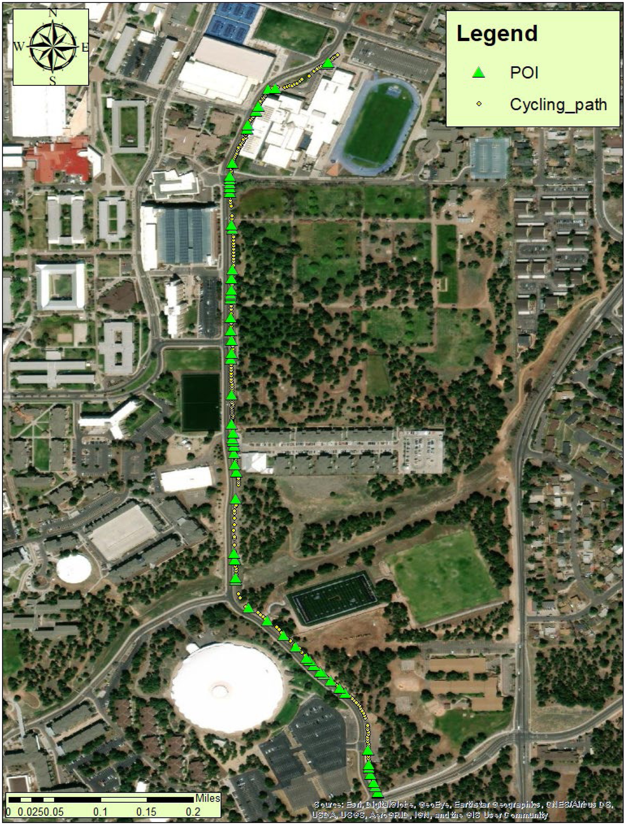
Fig. 7. Anomaly detection and localization in a GIS map. POI = point of interest known as an anomaly along the bike route.
(Base map sources: Esri, DigitalGlobe, GeoEye, Earthstar Geographics, CNES/Airbus DS, USDA, USGS, AeroGRID, IGN, and the GIS User Community.)
Field Validation (Multiple Cyclists)
After the preliminary test was done, the team recruited four cyclists (including men and women) and had each one of them travel on the two selected bike routes using their individual instrumented bike including street bikes and mountain bikes. The two bike routes are located on the west side of the campus where a variety of pavement distress patterns (potholes, cracks, bumps, etc.) are noticeable. Pavement surfaces that remain in good condition are collected for training purposes. Both pavements are made of asphalt materials. The field validation was designed to further evaluate the usefulness and effectiveness of the proposed LSTM-based sliding window computing algorithm in the identification of anomalies along the two bike routes. Each cycling trip generated a variety of vibration patterns based on the speeds, bikes, and individual cyclists. All patterns generated by instrumented cycling were normalized and analyzed using the LSTM-based sliding window computing algorithm to screen all vibration patterns and select anomaly candidates. The computing principle is that even though different cyclists and bikes would result in varying magnitudes of vibration patterns, the LSTM-based sliding window computing algorithm will be able to distinguish the dramatic change of vibration signals, recognize those patterns, and pick them as potential anomalies.
After each one of the four cyclists completed individual cycling on the two selected bike routes, all data were wirelessly transferred to the mobile apps and also stored in the sensor loggers. The team exported all data from the sensor loggers and mobile apps and transferred them to the computer for analysis. Using the LSTM-based sliding window computing algorithm, the patterns of potential anomalies of each cyclist were screened and identified (Figs. 8 and 9) and their georeferenced locations were displayed in GIS maps (Figs. 10 and 11). As can be seen in Figs. 8 and 9, the magnitude of the normalized vibration patterns against the number of data points fluctuates depending on the individual cycling. Based on the data, it can be concluded that the LSTM-based sliding window computing algorithm has been able to screen all normalized vibration patterns and identify potential anomalies (squared in red colors). As shown in Figs. 8 and 9, the selected anomalies are shown against the number of data points (in X-axis), so it is still hard to tell if those georeferenced anomalies collected from individual cyclists can represent the actual or closer pavement distress areas on the two bike routes. A field observation trip was then scheduled to compare the computing results with the identified pavement distress areas.
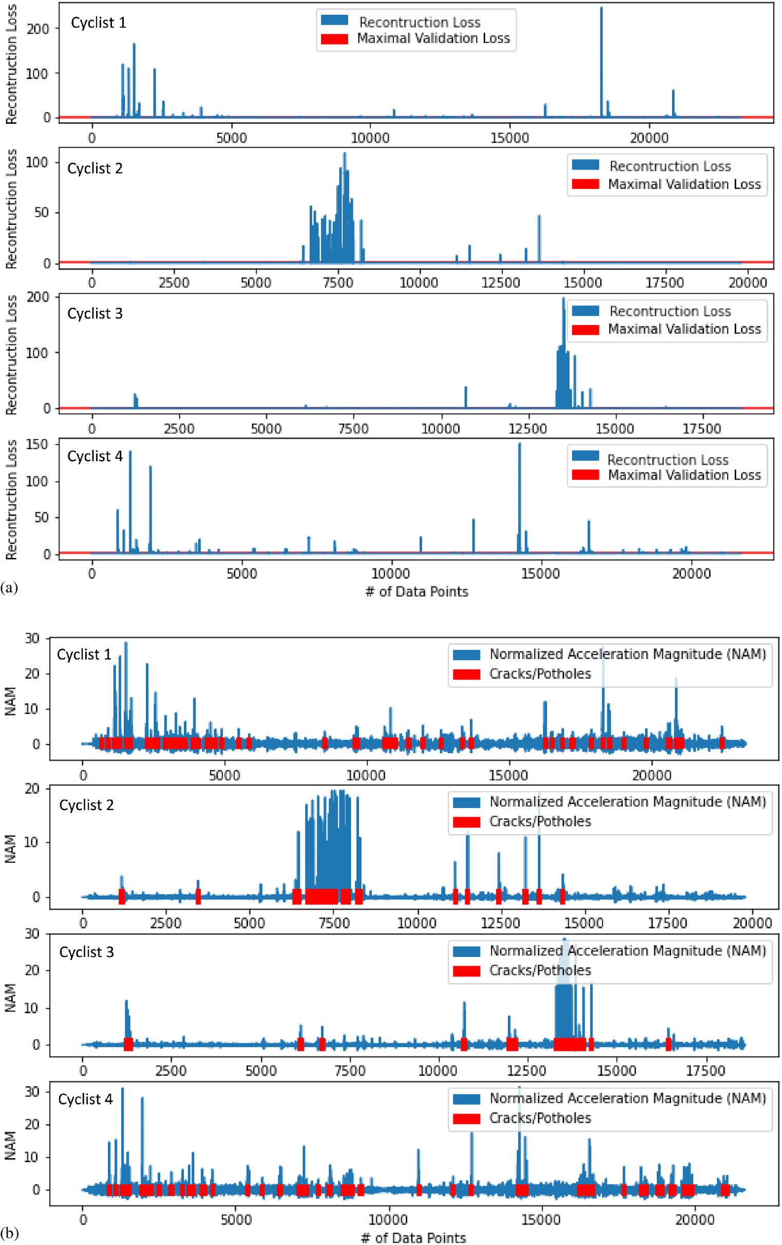


Fig. 10. Locations of identified anomalies on Bike route 1.
[Base map sources: Esri, HERE, Garmin, USGS, Intermap, INCREMENT P, NRCan, Esri Japan, METI, Esri China (Hong Kong), Esri Korea, Esri (Thailand), NGCC, © OpenStreetMap contributors, and the GIS User Community.]
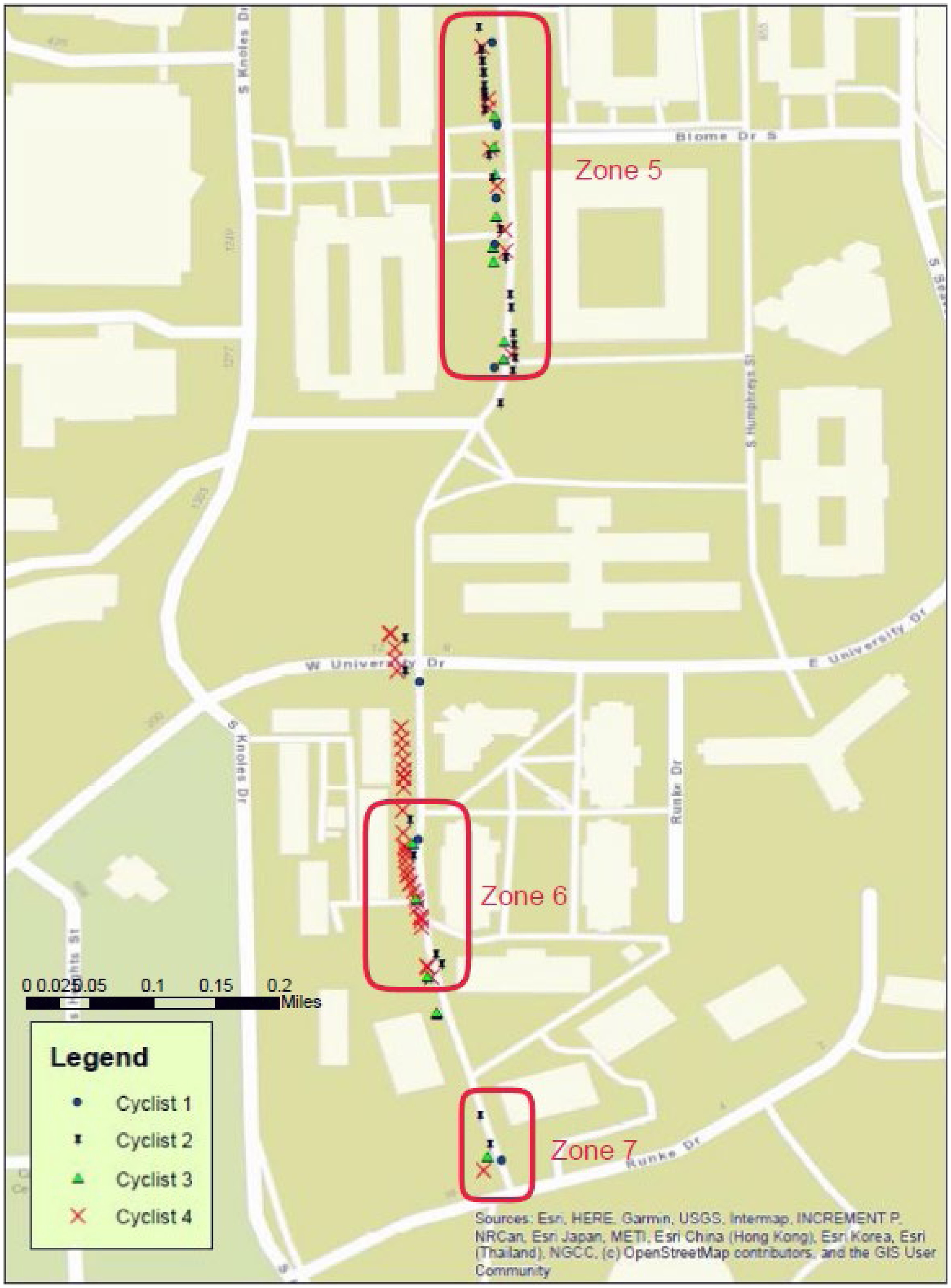
Fig. 11. Locations of identified anomalies on Bike route 2.
[Base map sources: Esri, HERE, Garmin, USGS, Intermap, INCREMENT P, NRCan, Esri Japan, METI, Esri China (Hong Kong), Esri Korea, Esri (Thailand), NGCC, © OpenStreetMap contributors, and the GIS User Community.]
Note that after reviewing the distributions of identified anomalies in the two GIS maps, the team rearranged all adjacent anomalies in a zone where all four instrumented cycling results have similar agreement in anomaly identification. These rearranged zones are useful to facilitate the evaluation. As shown in Fig. 10, there are four zones (Zones 1–4; highlighted in red lines), while three other zones are shown in Fig. 11 (Zones 5–7; highlighted in red lines). Additionally, there are a few anomalies beyond the highlighted seven zones that resulted from only one or two instrumented cycles. This is because the level of pavement distress is in a range of good to fair or the individual cycling paths did not travel onto the deteriorated areas. The team further retrieved anomaly data from GIS software and analyzed the results as provided in Table 2. A follow-up ANOVA test was performed to determine if the difference in anomaly detection among the four cyclists was significant and the result is provided in Table 3. A p-value of 0.98 > 0.05 was calculated from the ANOVA test, so the team concludes the difference in anomaly detection among the four cyclists is not significant. The ANOVA test supports the truth that the LSTM-based sliding window computing algorithm can effectively detect anomalies of cycling trails.
| Cyclist | Zone 1 | Zone 2 | Zone 3 | Zone 4 | Zone 5 | Zone 6 | Zone 7 | Total anomalies |
|---|---|---|---|---|---|---|---|---|
| Cyclist 1 | 1 | 4 | 10 | 12 | 17 | 7 | 2 | 53 |
| Cyclist 2 | 3 | 4 | 9 | 13 | 14 | 7 | 1 | 51 |
| Cyclist 3 | 3 | 3 | 7 | 11 | 13 | 8 | 1 | 46 |
| Cyclist 4 | 2 | 3 | 7 | 13 | 16 | 6 | 1 | 48 |
| Source of variation | SS | df | MS | F | P-value | F crit |
|---|---|---|---|---|---|---|
| Between groups | 4.142857143 | 3 | 1.380952381 | 0.049785408 | 0.984947061 | 3.00878657 |
| Within groups | 665.7142857 | 24 | 27.73809524 | — | — | — |
| Total | 669.8571429 | 27 | — | — | — | — |
The team went on to the two bike routes and observed the pavement distress conditions in the seven zones. The purpose of the field observation was to determine what levels of pavement distress areas have caused the bike routes to deteriorate and how accurately the LSTM-based sliding window computing algorithm was able to identify these deteriorated pavement areas. To systematically record the level of pavement distress areas on the two bike routes and relate the pavement distress to the accuracy of the LSTM-based sliding window computing algorithm, a rating handbook, the Distress Identification Manual, published by the Federal Highway Administration (FHWA 2014) was used for rating guidance when recording the severity level of the pavement (i.e., good, moderate, and high) on the two bike routes. The Distress Identification Manual provides a very detailed definition and explanation of each type of pavement distress, such as to how to identify distress types and rate a level of corresponding pavement distress. Based on the two GIS maps, the team walked through the two bike routes, rated each one of the pavement distress areas according to the Distress Identification Manual, and recorded the results in a field notebook. An example of pavement distress identification and rating results on the seven zones within the two bike routes is shown in the Appendix.
Based on the rating results, it is obvious that any pavement distress labeled as high or in some cases moderate in the severity level would lead to the generation of significant patterns by all cyclists. Another situation observed in the field is that some pavement distressed areas labeled as moderate or low might not generate recognizable patterns by all cyclists. This is because of the different paths of cycling and less significant vibration responses that were not selected by the LSTM-based sliding window computing algorithm. From the maintenance standpoint, the ignorance of low or moderate pavement distress areas during the computing process is acceptable as these mild pavement distress surfaces would not create cycling discomfort and raise a flag for maintenance. Instead, all pavement distress areas labeled as high in the rating book (Table 1) and in Figs. 9 and 10 exhibit adverse cycling conditions that have jeopardized cycling safety and mobility. More importantly, these cycling results call for the immediate attention of local authorities for maintenance or repair as well as provide useful information to be shared with cyclists, allowing them to navigate their trip and adjust routes (if needed) before cycling.
Summary
Given the results presented in Figs. 7‒10 along with the pavement rating record in the Appendix, regardless of the weight of the cyclists, speeds, bikes being used, etc., the LSTM-based sliding window computing algorithm is capable of screening and analyzing vibration patterns and identifying anomalies that could adequately reflect pavement distressed areas on bike routes. The identified anomaly locations and information can be shared with: (1) local authorities for decision-making for maintenance or repair; and (2) cyclists who will be able to plan their cycling trip accordingly. The use of the LSTM-based sliding window algorithm will advance the use of instrumented bikes and will be a good starting step to encourage the public to participate in crowd-sourcing-based cycling activities and collect more real-time cycling data for the improvement of cycling facilities. The rating record provides good information on the pavement condition assessment. Local authorities could take the record into account for policy decision-making for maintenance and prioritizing pavement distressed areas for repair. The results presented in the paper will be helpful in support of the advancement of instrumented bikes, improving cycling safety, and promoting cycling as a daily mode of transportation. The team is confident that the LSTM-based sliding window algorithm can replace our previous human-made threshold setting to classify pavement distress. For the future implementation of smart cycling using instrumented bikes, the LSTM-based sliding window will be highly recommended to be used as an advanced computing method for anomaly detection along bike trails.
Implication of Instrumented Bikes for Future Applications
Future applications will be continued on an array of roadway surfaces along bike trails including asphalt, concrete, gravel, and cobblestone sections under different weather conditions (dry, wet, and icy) to further evaluate the accuracy of the LSTM-based sliding window computing algorithm in anomaly detection along bike trails and lanes.
Conclusions
Through the demonstration of the LSTM-based sliding window computing algorithm in support of cycling activities, the paper has the following conclusions:
1.
The LSTM-based sliding window computing algorithm shows effectiveness in analyzing vibration patterns and identifying anomalies of cycling trails without any human-controlled supervision.
2.
From the practice standpoint, the cycling results bring immediate attention to local authorities for maintenance or repair as well as provide useful information to be shared with cyclists, enabling them to navigate their trip and adjust routes (if needed) prior to cycling.
3.
The LSTM-based sliding window computing algorithm can be a good technique to replace the currently used threshold setting for the determination of anomalies and promote the use of cycling as a daily mode of transportation.
4.
For future implementation, it is recommended that the LSTM-based sliding window algorithm be used on different road surfaces (e.g., asphalt, concrete, gravel, and cobblestone) under the effect of different weather conditions (dry, wet, and snowy).
Appendix. Examples of Pavement Distress Identification
Fig. 12 shows examples of pavement distress identification on selected Zones 1–7 within Bike routes 1 and 2.


Fig. 12. Examples of pavement distress identification in Bike routes 1 and 2.
(Images by authors.)
Data Availability Statement
Some or all data, models, or codes generated or used during the study are proprietary or confidential in nature and may only be provided with restrictions, including sensor logger programming, GUI coding, vibration data sets, Excel files, and GIS mapping data. Data requests will be approved at the corresponding author’s discretion.
Acknowledgments
The authors acknowledge the financial support by the University Transportation Center Pacific South Region.
References
Abbaspour, S., F. Fotouhi, A. Sedaghatbaf, H. Fotouhi, M. Vahabi, and M. Linden. 2020. “A comparative analysis of hybrid deep learning models for human activity recognition.” Sensors 20 (19): 5707. https://doi.org/10.3390/s20195707.
AMR (Allied Market Research). 2021. Accessed February 2021. https://www.alliedmarketresearch.com/connected-car-market.
Bayer, J. S. 2015. “Learning sequence representations.” Ph.D. thesis, School of Computation, Information and Technology, Technische Universität München.
Bengio, Y., A. Courville, and P. Vincent. 2013. “Representation learning: A review and new perspectives.” IEEE Trans. Pattern Anal. Mach. Intell. 35 (8): 1798–1828. https://doi.org/10.1109/TPAMI.2013.50.
Bengio, Y., P. Simard, and P. Frasconi. 1994. “Learning long-term dependencies with gradient descent is difficult.” IEEE Trans. Neural Networks 5 (2): 157–166. https://doi.org/10.1109/72.279181.
Dalal, N., and B. Triggs. 2005. “Histograms of oriented gradients for human detection.” In 2005 IEEE computer society conference on computer vision and pattern recognition (CVPR'05), Vol. 1, 886–893.
ECF (European Cyclists’ Federation). 2021a. “Smart Cycling Series: Big data and artificial intelligence are transforming bicycle navigation.” Accessed June 2021. https://ecf.com/news-and-events/news/smarter-cycling-series-big-data-and-artificial-intelligence-are-transforming-1.
ECF (European Cyclists’ Federation). 2021b. “Smart Cycling Series: you are what you share.” Accessed June 2021. https://ecf.com/news-and-events/news/smarter-cycling-series-you-are-what-you-share.
FHWA (Federal Highway Administration). 2014. Distress identification manuel. FHWA-HRT-13-092. Washington, DC: FHWA.
Hammerla, N. Y., S. Halloran, and T. Plötz. 2016. “Deep, convolutional, and recurrent models for human activity recognition using wearables.” Preprint, submitted April 29, 2015. http://arxiv.org/abs/1604.08880.
Ho, C.-H., J. Gao, M. Snyder, and P. Qiu. 2021. “Development and application of instrumented bicycle and its sensing technology in condition assessments for bike trails.” J. Infrastruct. Syst. 27 (3): 04021027. https://doi.org/10.1061/(ASCE)IS.1943-555X.0000632.
Ho, C. H., P. Qiu, S. Wen, X. Liu, M. Snyder, and K. Winfree. 2019. “Development of instrumented bicycle and mobile applications to perform cloud-based pavement condition management for bike roads.” In Proc., of 2019 Annual Conf. of Transportation Research Board. Washington, DC: Transportation Research Board.
Leitner, T., H. Kirchsteiger, H. and Trogmann, and L. del Re. 2014. “Model based control of human heart rate on a bicycle ergometer.” In Proc., European Control Conf. 1516–1521. Piscataway, NJ: Institute of Electrical and Electronics Engineers (IEEE).
Liu, X., C. Xiang, B. Li, and A. Jiang. 2015. “Collaborative bicycle sensing for air pollution on roadway.” In Proc., 2015 IEEE 12th Int. Conf. on Ubiquitous Intelligence and Computing, 316–319. Piscataway, NJ: Institute of Electrical and Electronics Engineers (IEEE).
Lu, N., N. Cheng, N. Zhang, X. Shen, and J. W. Mark. 2014. “Connected vehicles: Solutions and challenges.” IEEE Internet Things J. 1 (4): 289–299. https://doi.org/10.1109/JIOT.2014.2327587.
Malhotra, P., A. Ramakrishnan, G. Anand, L. Vig, P. Agarwal, and G. Shroff. 2016. “LSTM-based encoder-decoder for multi-sensor anomaly detection.” Preprint, submitted July 1, 2016. http://arxiv.org/abs/1607.00148.
Pedotti, L. A. S., R. M. Zago, and F. Fruett. 2016. “Instrument based on MEMS accelerometer for vibration and unbalance analysis in rotating machines.” In Proc., 1st Int. Symp. on Instrumentation Systems, Circuits and Transducers, 25–30. Piscataway, NJ: Institute of Electrical and Electronics Engineers (IEEE).
Pienaar, S. W., and R. Malekian. 2019. “Human activity recognition using LSTM-RNN deep neural network architecture.” In Proc., 2019 IEEE 2nd Wireless Africa Conf, 1–5. Piscataway, NJ: Institute of Electrical and Electronics Engineers (IEEE).
Pigatto, A. V., K. O. A. Moura, G. W. Favieiro, and A. Balbinot. 2016. “A new crank Arm based load cell, with built-in conditioning circuit and strain gages, to measure the components of the force applied by a cyclist.” In Proc., 38th Annual Int. Conf. of the IEEE Engineering in Medicine and Biology Society, 1983–1986. Piscataway, NJ: Institute of Electrical and Electronics Engineers (IEEE).
Qiu, P., X. Liu, S. Wen, Y. Zhang, K. Winfree, and C. H. Ho. 2018. “The development of an IoT instrumented bike: For assessment of road and bike trail conditions.” In Proc., Int. Symp. in Sensing and Instrumentation in IoT Era, 1–6. Piscataway, NJ: Institute of Electrical and Electronics Engineers (IEEE).
Sermanet, P., D. Eigen, X. Zhang, M. Mathieu, R. Fergus, and Y. LeCun. 2013. “Overfeat: Integrated recognition, localization and detection using convolutional networks.” Preprint, submitted December 21, 2013. http://arxiv.org/abs/1312.6229.
Srivastava, N., E. Mansimov, and R. Salakhudinov. 2015. “Unsupervised learning of video representations using lstms.” In Proc., Int. Conf. on Machine Learning, 843–852. New York: Association for Computing Machinery.
Zhao, Y., R. Yang, G. Chevalier, X. Xu, and Z. Zhang. 2018. “Deep residual bidir-LSTM for human activity recognition using wearable sensors.” Math. Probl. Eng. 2018: 7316954.
Information & Authors
Information
Published In

ASCE OPEN: Multidisciplinary Journal of Civil Engineering
Volume 2 • Issue 1 • April 2024
Copyright
This work is made available under the terms of the Creative Commons Attribution 4.0 International license, https://creativecommons.org/licenses/by/4.0/.
History
Received: Sep 4, 2023
Accepted: Jan 17, 2024
Published online: Apr 15, 2024
Published in print: Apr 15, 2024
Discussion open until: Sep 15, 2024
Authors
Metrics & Citations
Metrics
Citations
Download citation
If you have the appropriate software installed, you can download article citation data to the citation manager of your choice. Simply select your manager software from the list below and click Download.