Economically Optimal Leak Management: Balancing Pressure Reduction, Energy Recovery, and Leak Detection and Repair
Publication: Journal of Water Resources Planning and Management
Volume 150, Issue 8
Abstract
Maximizing the net economic benefits of leak management programs provides the most value to water utilities and their customers. Leak management programs with alternative objectives (e.g., to “break even” or to maximize leak reduction) are not necessarily the most efficient use of resources. Combining hydraulic modeling with principles of economics and using a real distribution system to provide a case study, we present a methodology for maximizing the net economic benefits of a leak management program consisting of leak detection and repair activities and pressure management interventions. The optimization results include recommended leak detection and repair intervals for individual district metered areas, optimal siting of both pressure reducing valves and pumps-as-turbines (PATs), and modifications to the distribution system’s connectivity to isolate high-pressure areas. The case study results indicate that 10% to 11% of the system’s current energy use can be recovered by PATs and that the avoided leakage over the study period is equivalent to 13% to 23% of the system’s current customer demand. While leak detection and repair and pressure management are more commonly considered independently, this analysis demonstrates the feasibility of including their interdependencies when optimizing a leak management program, resulting in more useful recommendations.
Introduction
Safe, reliable, and affordable potable water is essential for social and economic prosperity. In many regions of the world, growing populations and arid conditions are straining water resources (Kunkel 2016; Liemberger and Wyatt 2019; Liu et al. 2022; Tzanakakis et al. 2020). In addition to efforts to reduce water consumption through conservation, water suppliers are obligated to accountably and efficiently manage their water resources (Kunkel 2016). The amount of water lost by water suppliers is known as nonrevenue water and consists of two types of losses: real and apparent (Sturm et al. 2008). Real losses include leaks, overflows, and blow-offs anywhere in the distribution system (Sturm et al. 2008). Apparent losses consist of water lost to theft or illegal use and water that is not physically lost but that fails to produce revenue due to inaccurate metering or other data errors (Sturm et al. 2008). Reducing real losses through leak management represents a significant opportunity for water suppliers to minimize waste and increase the supply of water available to customers (Rupiper et al. 2022). For example, water audit data for 882 water suppliers in the United States revealed that water lost to leaks on average accounted for 17% of the total water produced, ranging from 1% to 55%, depending on the supplier (Rupiper et al. 2022). Globally, leakage rates may range from approximately 4% in Amsterdam to 65% in Tuxtia, Mexico (OECD 2016). Awareness of the need to monitor and mitigate leak losses is now widespread, with many countries considering measurement and control programs (Rupiper et al. 2022).
The three main activities that water suppliers may use to reduce leak losses are leak detection and repair, pressure reduction, and preventative pipe replacement (Lambert and Fantozzi 2005). Although necessary for long-term maintenance of a water distribution network, preventative pipe replacement is generally not cost-effective from the perspective of reducing leaks (Rupiper et al. 2022; Trow and Farley 2004). Recent work suggests that pressure reduction and leak detection and repair may be the most affordable ways to increase the available water supply compared with common alternatives (e.g., purchasing additional water) (Rupiper et al. 2022). Leak detection is a broad field of research that has led to the development of technologies that take advantage of acoustic, pressure transient, vibrational, flow, and other types of data to locate leaks in water distribution networks (Hu et al. 2021). For example, acoustic methods may use ground microphones, leak noise correlators, and noise loggers, while other methods include ground-penetrating radar and thermal infrared imaging (Fan et al. 2022). After detecting and locating leaks, the water supplier may take corrective action to prevent further water loss.
Pressure management aims to reduce pressures to the minimum levels required to provide adequate service. Water suppliers may be required to provide higher pressure than necessary to many customers to ensure that all service connections receive adequate pressure. For example, customers at lower elevations will likely receive higher pressure than customers at higher elevations within a district metered area (DMA), which is sometimes referred to as a “pressure zone.” Alternatively, pump stations may sometimes provide more pressure than is necessary to an entire DMA for other reasons. In either case, greater pressures result in greater leak losses, which water suppliers have traditionally managed using pressure reducing valves (PRVs) placed at strategic locations within the distribution system. However, the energy dissipated in PRVs can instead be captured by pumps operating in reverse as turbines (PATs) with an attached generator. Depending on the energy recovery potential, PATs may sometimes be more economical than PRVs. Determining where to place PRVs and PATs within a distribution network has been the focus of significant recent research efforts. Research objectives have included maximizing energy recovery (Carravetta et al. 2012; Corcoran et al. 2016; van Dijk et al. 2022; Fernández García and Mc Nabola 2020; Giugni et al. 2014; Lima et al. 2017a; Moazeni and Khazaei 2021; Morani et al. 2023; Telci and Aral 2018); multiobjective optimization of energy recovery and leak reduction (Bonthuys et al. 2020; Ebrahimi et al. 2021; Fecarotta and McNabola 2017; Morani et al. 2021; Sambito et al. 2021); cost–benefit analysis (Carravetta et al. 2014; Fecarotta et al. 2015); case studies (Novara and McNabola 2021; Patelis et al. 2017; Su and Karney 2015); PAT selection, design, and operation (Alberizzi et al. 2019; Amelio et al. 2020; Bideris-Davos and Vovos 2023; Fontanella et al. 2020; Lima et al. 2017b; Lydon et al. 2017; Pugliese and Giugni 2022; e Souza et al. 2023; Stefanizzi et al. 2020); and capacity assessment (Kao et al. 2022). Although previous studies have used economics and hydraulic modeling to determine the optimal placement of PRVs and PATs, here we recognize that, because the amount of water saved by a leak detection and repair program is dependent on the operating pressure, the placement of PRVs and PATs should take place within the context of a more complete leak management program.
To provide maximum value to customers, leak management programs should be operated at the economically efficient level of losses (i.e., the level of leakage beyond which leak reduction is no longer the best financial choice for increasing the supply of available water) (Rupiper et al. 2022). To achieve this, the net benefits provided by leak reduction efforts should be maximized. While the economic model given by Rupiper et al. (2022) is adequate for making general comparisons and producing broad conclusions involving a large number of organizations, we suggest several modifications to improve the usefulness and rigor of the model when applied to a specific water distribution system. First, rather than assuming baseline pressure reduction benefits and independently optimizing leak detection and repair operations, we optimize both activities simultaneously and include their interdependencies. Second, we utilize the hydraulic model of a real water distribution system to propose detailed modifications to the distribution system to reduce pressures. Third, we consider the use of PRVs and PATs for pressure reduction and energy recovery. We apply these methods to a portion of the distribution network operated by Marin Municipal Water District (hereafter referred to as Marin), a water supplier serving 191,000 people in Northern California, and provide the results as a case study for other utilities seeking to manage their leaks more efficiently and economically through optimizing the placement of PRVs and PATs and the frequency of leak detection surveys.
Methods
Determining the financially optimal leak management policies and operations requires economic and engineering principles. Hydraulic modeling is required because the costs and benefits of leak detection and repair and pressure reduction are interdependent. For example, if the pressure in a DMA is reduced, the benefits of surveying for leaks are reduced. Conversely, if leak detection and repair are performed more frequently, the benefits of pressure reduction are reduced. Hydraulic modeling accurately describes how such modifications to system operation impact the results. Economic principles are necessary to understand the true costs and benefits of leak management activities so that economically efficient solutions may be found.
Hydraulic Modeling
Hydraulic models of water distribution systems solve systems of equations based on the principles of energy and mass conservation to estimate variables of interest to engineers and operators, including flow, velocity, and hydraulic head and provide valuable assistance for the planning, design, and operation of hydraulic pipelines (Walski et al. 2013, 2020). Marin’s distribution network conveys approximately () of water per day through 1,461 km (908 mi) of mains and approximately 64,000 service connections. For this analysis, a hydraulic model for the city of Sausalito, in Marin’s southwest service region, was constructed using EPANET Version 2.2, the industry-standard hydraulic modeling simulation toolset (Rossman 2000; USEPA 2020). The model was skeletonized and calibrated to a seven-day period in the summer of 2019, identified by Marin as typical and without operational disturbances or changes. The model includes 33.67 km (20.92 mi) of distribution pipes with an average diameter of 20.3 cm (8 in.) and is supplied by a single reservoir representing the rest of Marin’s network. A total of 19 valves, 12 pumps, and 8 storage tanks are distributed within the model to provide water service to 904 junctions.
Elevations of junctions in the Sausalito model range significantly from a minimum of 2.7 m (9 ft) to a maximum of 300.8 m (987 ft), with an average of 67.4 m (221 ft). Average service pressures range from 614 to 676 kPa (89 to 98 psi), and junction pressures in the model agree with known hydrant pressures within () for 90% of the hydrants and within () for the rest, excluding a small number of outliers, which could not be explained with the modeled hydraulics. Customer water demand was generated from monthly bills and assumed time-series patterns for each customer class such that total usage matches the observed hourly total system water production. Between the valves and pumps, a total of nine isolated service regions, or DMAs, were identified by their connectivity. Valves, pumps, other infrastructure, and their associated properties (e.g., energy demand or production) are considered as belonging to a DMA only if they are upstream. Each DMA has its own service pressure range, which varies principally based on elevation and distance from the nearest storage tank. A winter 2019 simulation was performed using the same model calibrated for summer 2019, reducing the system-wide demand multiplier from 1.0 to 0.573, which was calculated by dividing the total volume of water sold in February of 2019 by that of August of 2019. For more information, see the Supplemental Materials.
Economic Modeling
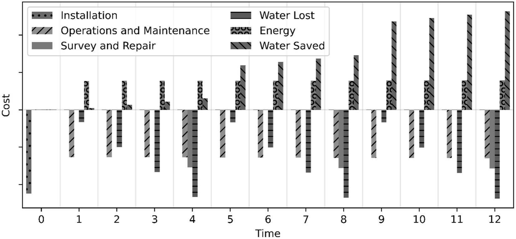
The benefits and costs of leak management activities were estimated for each month of the project life (30 years), as illustrated in Fig. 1. The net present value was calculated by discounting future values according towhere is assumed to be 4% per annum. Accordingly, expected future values were calculated aswhere = the expected rate of growth in the cost. All equations used to estimate costs were adjusted to the present based on their year of publication using an average inflation rate of 2.5% per annum.
(1)
(2)
Pumps-as-Turbines
The costs of PATs and their associated generators were determined using empirical formulas developed by Novara et al. (2019) and methods used by Mitrovic et al. (2021). The cost of the PAT and generator is given aswhere = an empirically determined coefficient (11,913.91); and () and (m) are the best efficiency point (BEP) flow and head loss through the PAT. Other installation costs (OIC) are given bywhere (0.26) = the fraction of the total installation cost represented by . Following Mitrovic et al. (2021), we assume that the operations and maintenance costs of PATs and their generators are 15% annually of their total installation costs (), with an annual growth rate () of 2.5% per annum.
(3)
(4)
Pressure Reducing Valves
The costs associated with PRVs include the capital cost of the valve itself, two gate valves, a strainer, and an air valve (Jones and Barkdoll 2022). The cost of PRVs and associated materials depends on the diameter of the valve, as given bywhere (cm) = the diameter of the valve; and (1,474.8), (0.0824), (500), (0.0658), (100.5), (300), (412.2), and (512) are empirically determined coefficients (Jones and Barkdoll 2022). The operations and maintenance costs for PRVs were assumed to be negligible over the lifetime of the project.
(5)
Survey and Repair Costs
The initial survey and repair costs assume that all leaks are repaired, reducing the unreported leakage rate to zero or the unavoidable annual real losses level. The cost of the initial survey and repair is given bywhere = the initial leakage; = the average leak flow rate; = the adjusted leak repair cost; = the full leak detection survey cost; and the initial leakage is assumed to be equivalent to Marin’s 2022 real losses (; 1,045 acre-ft), as reported to the California Department of Water Resources [the data are available through the Water Use Efficiency Data Portal (WUEdata - Public Portal, n.d.)]. The rate of growth of the costs ( and ) are assumed to be 2.5% per annum. The cost of surveying and repairing leaks after the initial survey and repair efforts is estimated aswhere = the number of time periods (months) between surveys; and = the rate of rise of unreported leaks. For more details, see the Supplemental Materials and Rupiper et al. (2022).
(6)
(7)
Water Lost
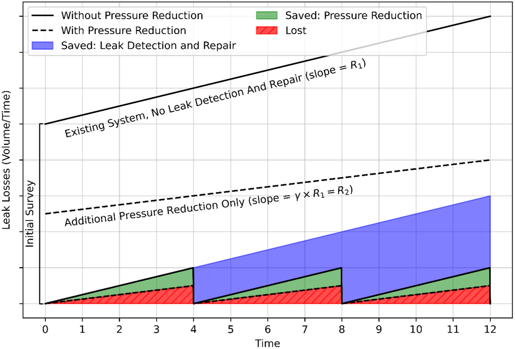
The volume of water lost during each month is calculated by integrating the leakage rate over time, as shown in Fig. 2, and given bywhere = the fraction of the leakage rate that remains after pressure reduction (see Fig. 2) and is defined following the leak model used by Rupiper et al. (2022) aswhere = the initial service pressure; = the new service pressure after an intervention; and = the pressure-leakage relationship exponent given bywhere ICF = the infrastructure condition factor; ILI = the infrastructure leakage index; and = the fraction of pipes in the network that are constructed of rigid materials [here assumed to be 0.75 following Rupiper et al. (2022) in absence of the data required to make a more accurate assumption]. The pressures are estimated by the hydraulic model for the junctions or the nearest service connection. For more details, see the Supplemental Materials in Rupiper et al. (2022). Note that the function describing the actual leakage rate over time is a piecewise function (see Fig. 2) since the leakage rate is reset to zero (or the level of unavoidable losses) whenever a survey and repair activity takes place. The amount of water lost was calculated individually for each month. The cost of water is given by the variable production cost (), which is specific to each utility. To estimate the value of the lost water (), we assume an annual growth rate for the variable production cost () of 2.5% per annum.
(8)
(9)
(10)
Energy Produced
The amount of energy produced by a PAT () is an output of the hydraulic model and is estimated using the relationshipwhere () = the flow; (m) = the head loss; () = the density of water; () = gravitational acceleration; and (0.76) = the PAT efficiency (which may be slightly lower than what is possible) (Giosio et al. 2015). To estimate the value of the energy recovered (), we assume an average energy sale price of $0.12 per kWh and a cost growth rate () of 2.5% per annum. The estimated weekly energy production for the summer and winter models was averaged and used to determine the average expected monthly energy production.
(11)
Avoided Leakage
The volume of avoided leakage is here defined as the difference between the water that would have been lost if no leak management activities had taken place after the first survey and repair activities (illustrated by the top line in Fig. 2) and the amount of water actually lost given the proposed leak reduction activities (illustrated by the bottom piecewise function in Fig. 2). The value of the avoided leakage () each month is determined using the same methods given here for lost water.
Optimization Algorithm
With the goal of maximizing the net economic benefits over the study period, the optimization algorithm generates new hydraulic models by placing PRVs and PATs and disconnecting pipes where appropriate to create new DMAs. The creation of new DMAs allows the optimization to isolate service areas with higher than necessary pressure to facilitate pressure reductions while maintaining minimum customer service pressures. The optimization was performed under summer conditions and subsequently applied to the winter model to obtain results for both seasons. We utilize the multithreaded simulation optimization platform programmed in C++ in Linz et al. (2020) to evaluate the model with a particle swarm optimization algorithm (Kennedy and Eberhart 1995). Particle swarm optimization is a population-based search algorithm, which explores an optimization’s domain with a set of moving policies that gravitate toward local and global optima simultaneously. This strategy allows for the resilient exploration of a solution space when faced with many local optima, such as in the domain of hydraulic model optimization. The platform developed in Linz et al. (2020) is utilized to schedule, manage, and progress the optimization logic across iterations, while utilizing any programmable, generalized objective function.
Each particle in the particle swarm optimization algorithm consists of a policy vector (), which we define as a set of values that indicate the changes to be made within the model. The values refer to a set of indexed pipes, pumps, or valves [], which are sorted geographically along a 2D Hilbert curve, such that small changes to a pipe index results in small changes to the geographic location of the installed PAT or PRV (Hamilton and Rau-Chaplin 2007). To make the optimization problem solvable with limited computational resources, the number of items in was limited to four, which corresponds to the maximum number of PRVs or PATs that may be added to the system. For example, the policy might be , which would indicate that the optimization would attempt to place PRVs and PATs at pipes 3, 6, 9, and 11. The optimization always compares the economic viability of PRVs and PATs and selects the more advantageous option for each pipe. The algorithm may also choose to place fewer than four devices. Based on the model simulation (), the relevant hydraulic quantities can be modeled as deterministic functions of the specific asset , the overall policy vector , and the selected timestep . Observable hydraulic outputs (e.g., energy, head loss, or flow) for a specific asset are given bywhere to is the time period over which the simulation occurs. Several components of the net benefits formula can be evaluated from the hydraulic model asandwhere = the total energy cost of the pumps in the network, which may change with the introduction of new infrastructure; = the energy demand of with the changes identified within from to ; = the value of the net energy recovered by the PATs installed in the distribution system given the set of changes indicated by ; and = the duration of the study period.
(12)
(13)
(14)
A fundamental requirement of operating water systems is to supply adequate water pressure to customers (typically, at least 275.8 kPa or 40 psi), prevent suction pressures within distribution pipes, and prevent water tanks from draining excessively. Thus, the optimization problem is defined aswhere = the value of the avoided leakage; = the value of the energy recovered; = the value of the water lost to leaks; = the cost of surveying and repairing leaks; = the cost of the initial survey and repair activity; = the cost of installing PATs and their associated generators; = the operations and maintenance cost for PATs and generators; = the value of the energy required to operate all pumps throughout the distribution system; and = the cost of installing pressure reducing valves. The optimization is subject to the constraintsandwhere = all customer pressures; = all nodal pressures; and = all tank levels. The pressure and tank level constraints are implemented as per-node or per-tank penalties that negatively impact the objective function with extremely large values for each constraint violation. Before the hydraulic simulation can be performed, each input vector is used to generate a new hydraulic model with new PATs or PRVs and potentially with pipe closures. The construction of a new model consists of several steps, including the following:
(15)
1.
Evaluate the full hydraulic simulation for the original network.
2.
Determine the DMAs for the original network.
3.
For each potential PAT or PRV location in :
a.
Replace the previous link with the new PAT or PRV in the model.
b.
Align the new PRV or PAT with the average flow direction of the original link .
c.
Set the PRV or PAT target downstream pressure to the average pressure of the node immediately downstream of the original link .
4.
For each new PAT or PRV location in :
a.
Try to find the shortest possible path connecting the upstream node to the downstream node for within link ’s current DMA, which does not utilize link .
(1)
If found, close the link in the middle of that path. Repeat this loop analysis until no path is found within the DMA that loops around the new PAT or PRV.
5.
Evaluate the DMAs for the new network.
a.
If any DMA is infeasible due to impossible network configurations or poor engineering practices, such as pumps looping on themselves or the lack of a water supply for storage tanks, then the decision vector is rejected early with a poor performance value.
6.
For each new PAT or PRV location in :
a.
Identify the minimum customer pressure () and node pressure () within the downstream DMA from the new link at .
(1)
If found, reduce the setting for the new PAT or PRV downstream pressure target until or would violate an optimization constraint [e.g., 275.8 kPa (40 psi) customer service pressure, empty tanks, or vacuum pressure].
7.
Evaluate the full hydraulic simulation for the new network.
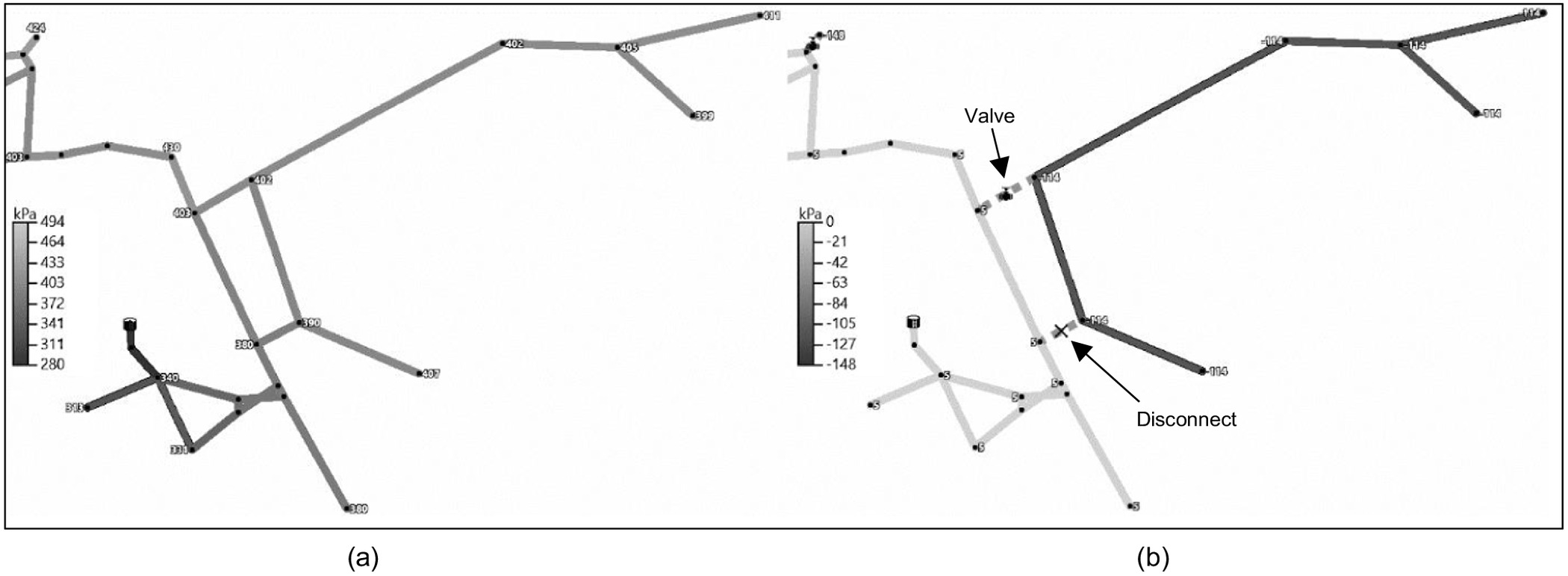
The particle swarm optimization algorithm was implemented with 500 particles and limited to 1,000 iterations based on an initial fitting exercise. At the conclusion of each particle evaluation, the decision on whether to place a PAT or PRV for each location is based on the maximized net benefit, as determined in Eq. (15). Each dimension of the vector represents a single potential installation site, and, due to the regional sorting with the Hilbert curve, small changes to the decision vector would result in only small changes to the objective function. Overall, this strategy was selected to reduce dimensionality to exactly the number of PATs or PRVs being placed simultaneously and to maximize the search potential of the particle swarm optimization algorithm and ensure it adequately explores the decision space. If no improvement in the objective function is observed in 100 iterations, the optimization terminates. The algorithm typically produces several new hydraulic pressure zones that are served by one to two PATs or PRVs, with pipe closures as necessary (see Fig. 3). The procedures described here were also performed using a genetic algorithm (GA) based on the approach described in Linz et al. (2020) but modified to include Newton’s method.
Results
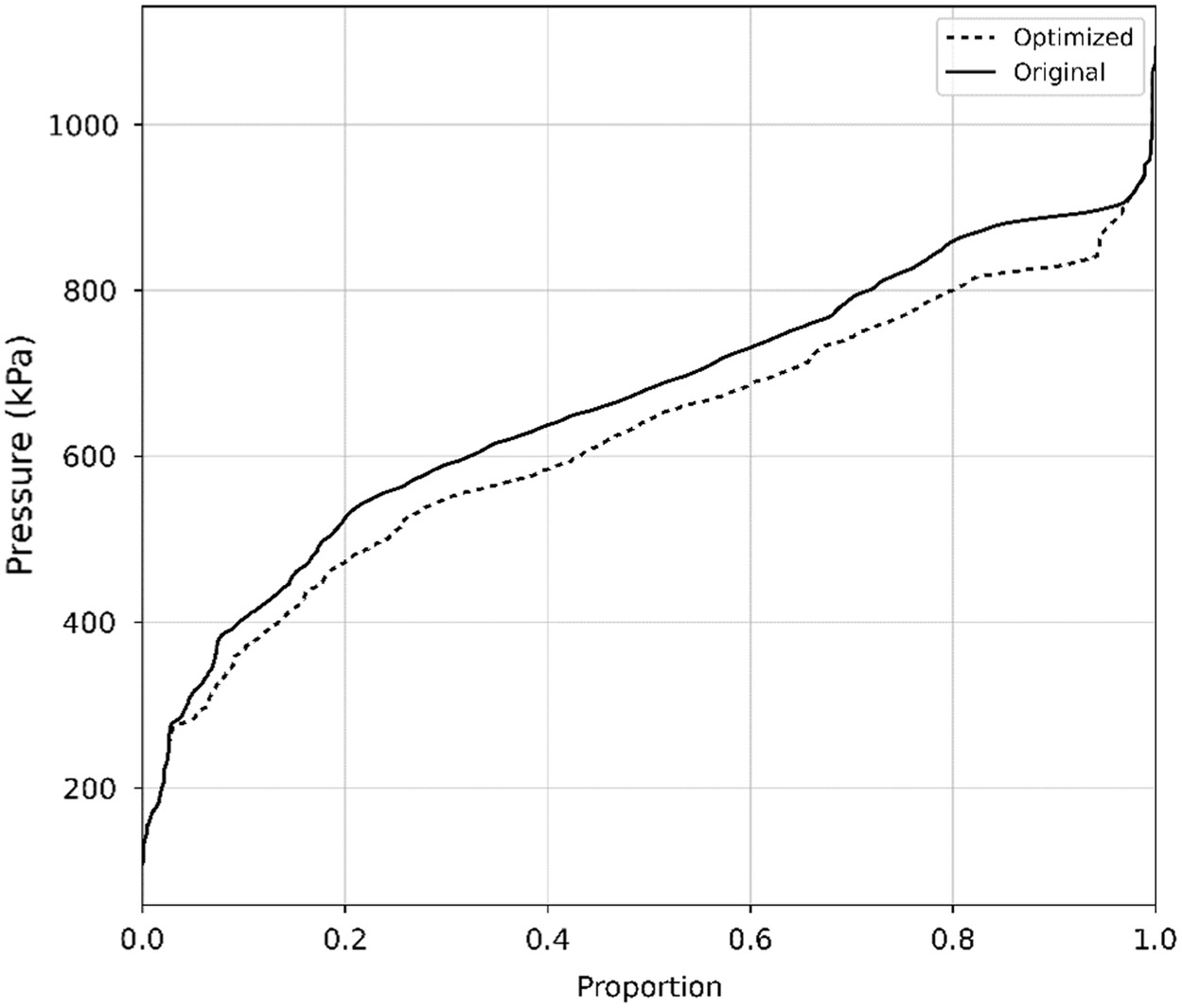
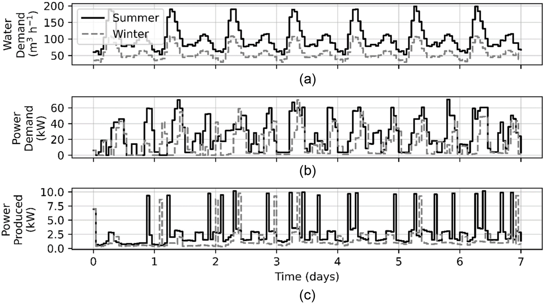
The particle swarm optimization resulted in the placement of four new PATs, the replacement of a throttle control valve with a PAT, a total water savings of (), average power production of 1.5 to 2.9 kW, and net economic benefits of over the 30-year study period. The particle swarm optimization algorithm terminated after 100 iterations without improvement before reaching the 1,000-iteration limit. As shown by the results in Table 1, all DMAs except one were suitable for PAT placement and leak reduction activities with positive net economic benefits. Four new DMAs were created during the optimization to maximize the potential benefits of pressure reduction strategies. Figs. 4 and 5 illustrate the estimated pressure changes throughout the distribution network resulting from the optimization. Considering all nodes during the summer and winter extended period simulations, the average pressure throughout the distribution system was reduced by 6.4% after optimizing. Fig. 6 shows the water demand, energy demand, and production for each DMA. The genetic algorithm optimization resulted in a different, but less optimal, distribution system configuration.
| DMAa | Average demand () | PRVb | PATc | Nodesd | Pipe length (m) | Average power demand (kW) | Average power produced (kW) | Survey interval (y) | Avoided leakage ( per 30 y)e | Net benefits ( per 30 y) |
|---|---|---|---|---|---|---|---|---|---|---|
| 1f,g | 0.4–0.6 | 0 | 0 | 2 | 16 | 1.6–3.2 | 0.0 | — | — | — |
| 2h,i | 127.9–221.3 | 0 | 1 | 55 | 2,467 | 0.0 | 0.3–0.6 | 2.2–2.8 | 264.2–269.2 | 55.5–56.1 |
| 3 | 0.6–3.5 | 0 | 0 | 1 | 151 | 0.0 | 0.0 | 5.1 | 2.5 | 0.2 |
| 4 | 429.0–770.6 | 0 | 0 | 149 | 7,364 | 3.6–6.6 | 0.0 | 1.6 | 1,012.8–1,014.2 | 214.1–214.4 |
| 5 | 110.0–201.7 | 0 | 0 | 49 | 3,080 | 2.0–3.7 | 0.0 | 2.2 | 325.5–328.1 | 66.6–67.3 |
| 6j | 4.9–6.3 | 0 | 0 | 1 | 96 | 6.2–10.1 | 0.0 | 15.1 | 0.9 | 0.2 |
| 7 | 12.0–30.1 | 0 | 0 | 9 | 474 | 0.1–0.3 | 0.0 | 2.8 | 29.2–29.4 | 5.3–5.4 |
| 8 | 70.5–114.9 | 0 | 0 | 31 | 1,732 | 0.6–0.9 | 0.0 | 2.8 | 162.1–163.1 | 32.6–32.9 |
| 9 | 74.9–137.1 | 0 | 0 | 22 | 1,214 | 0.8–1.5 | 0.0 | 2.2 | 128.2–129.3 | 26.2–26.5 |
| 10f | 6.0–11.0 | 0 | 2k,l | 3 | 115 | 0.0 | 0.2–0.5 | 10.1 | 5.4 | 1.4 |
| 11f | 219.6–380.4 | 0 | 1k | 83 | 3,420 | 0.0 | 0.3–0.5 | 2.8 | 412.4–413.9 | 93.3–93.5 |
| 12f,i | 626.6–1,111.6 | 1m | 1k | 240 | 11,641 | 0.0 | 0.7–1.3 | 1.6 | 1,993.5–2,000.6 | 441.3–443.3 |
| 13 | 17.2–29.8 | 2m | 0 | 1 | 8 | 0.0 | 0.0 | 2.8 | 0.6 | 0.1 |
| 14d | 0.0–0.0 | 2m | 0 | 0 | 5 | 0.0 | 0.0 | 2.8 | 0.4 | 0.1 |
Note: Valves and pumps are considered as belonging to a DMA only if they are upstream.
a
District metered area.
b
Pressure reducing valve.
c
Pump-as-turbine.
d
Customer nodes.
e
For example, .
f
Created during optimization.
g
No beneficial leak detection and repair strategy were identified.
h
Pipe length reduced by 1.7% during optimization.
i
Winter avoided leakage is higher than summer; the opposite is true for all others.
j
Pipe length reduced by 99.4% during optimization.
k
Placed by optimization.
l
One PAT replaced a throttle control valve.
m
Preexisting.
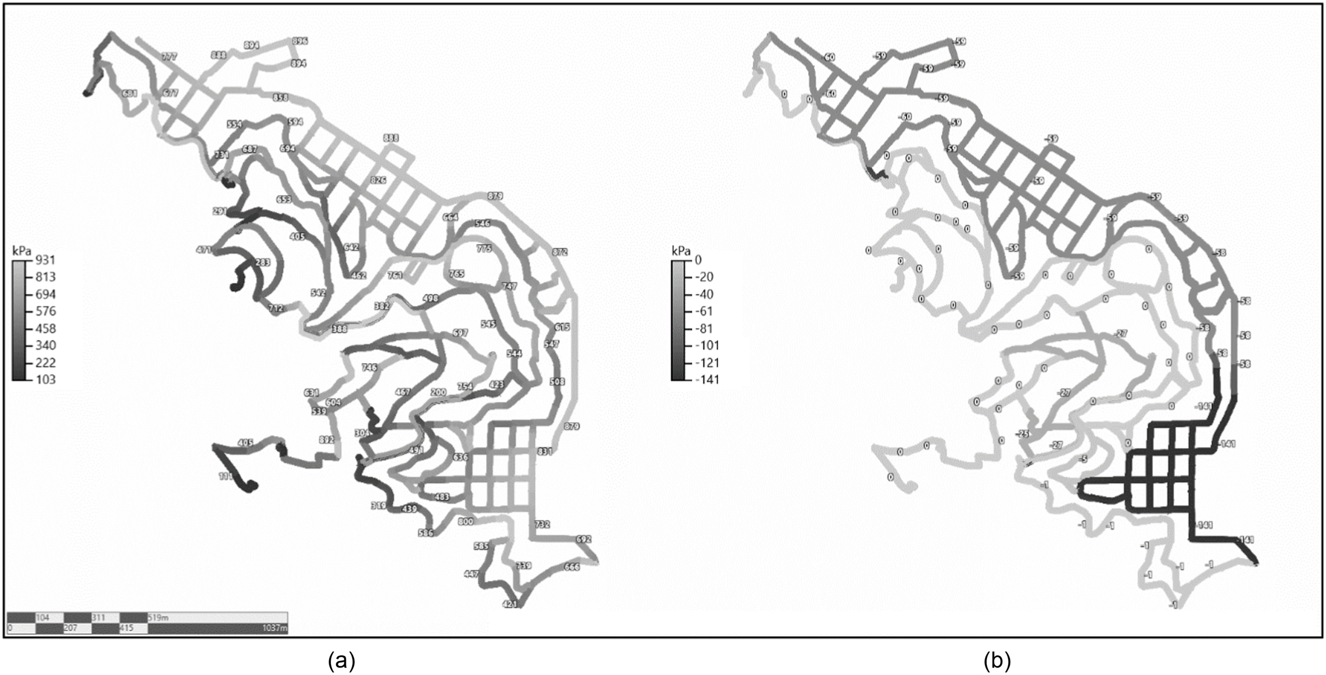
Discussion
The particle swarm optimization successfully reduced pressures throughout the distribution network. As shown in Fig. 4, pressure reductions occur mainly between 275.8 to 896.3 kPa (40 to 130 psi). Pressures below 275.8 kPa (40 psi) were not significantly reduced due to minimum customer pressure requirements, while pressures above 896.3 kPa (130 psi) are likely associated with too little flow to make energy recovery and pressure reduction economically feasible. Fig. 5 shows the spatial distribution of pressure reductions and indicates that reductions of average pressure as high as 137.9 kPa (20 psi) occur in a significant portion of the distribution network. Although some areas of the network increased in pressure, the heatmap shown in Fig. 5 considers only pressure reductions because areas where pressures increased are so small, they cannot be seen. The lowest pressures observed in the distribution network likely belong to junctions located near tanks, which tend to occur at higher elevations and feed into DMAs without assistance from pumps, leading to lower pressures for customers immediately adjacent to the tanks. For this reason, customers are typically either not connected to DMAs with tanks at their elevation or pumps are used to lift water stored in tanks to the target hydraulic grade lines. High pressures within the distribution network are mostly along the coastline and are associated with significant elevation change within the DMA. Pressure reductions were the result of the placement of five PATs and the creation of four new DMAs to restrict flow and isolate high-pressure areas. Of the five preexisting PRVs, none were converted to PATs (due to modeling constraints, PRVs could not be removed). It appears that, in locations where additional pressure management was feasible, PATs were more economically viable than PRVs. As shown in Table 1, the total estimated energy recovery by PATs is equivalent to 10% to 11% of the current energy requirements (i.e., energy required for pumping). As shown in Fig. 6, peak energy recovery generally aligns with peak water demand. The additional energy required to pump water lost to leaks if no leak management activities were implemented is not included here, though it would likely be significant over the 30-year study period.
The particle swarm optimization also successfully identified the optimal leak survey intervals for 13 out of the 14 DMAs, ranging from 1.6 to 15.1 years between survey and repair activities. Performing the analysis at the DMA level allows for greater precision in targeting areas where fixing leaks is more valuable. Survey and repair activities in combination with pressure reduction are estimated to prevent a significant amount of leakage over the study period, equivalent to 13% to 23% of current customer demand. This does not mean that customer demand would be reduced by 13% to 23%. Rather, this is the equivalent amount of water that would be lost if leak management activities were not implemented over the study period. This value does not include the benefits of the initial surveys and repairs over the study period, as shown in Fig. 2, and is thus a more conservative estimate. Because the hydraulic model used for this analysis is demand (as opposed to pressure) driven, determining reductions in customer demand due to interventions is not feasible.
Leak detection and repair, pressure management, and energy recovery are generally considered independently in leak management programs and optimizations found in the literature. However, because implementing either strategy alters the hydraulic characteristics of a distribution system, they are interdependent and should be optimized together. Although doing so is more challenging, the results are more realistic and useful for water utilities. This analysis demonstrates the feasibility of considering both approaches simultaneously using hydraulic modeling and economics and provides a case study for water utilities considering a similar approach. However, these results are sensitive to model assumptions, and more rigorous quantification of model inputs (e.g., survey and repair costs) is recommended when applying this methodology in practice. This may require increased data collection efforts by water utilities to better understand relevant system characteristics (e.g., the rate of rise of leaks). Additionally, because the results are only as reliable as the hydraulic model on which the analysis is based, only calibrated and proven models should be used.
Although the particle swarm optimization provided a positive result and measures were taken to increase confidence in the solution, as with all heuristic optimization algorithms applied to complex problems, we cannot be certain that the global optimum was found. Other optimization algorithms may recommend alternative distribution system configurations due to differences in how they navigate the solution space. For example, the genetic algorithm optimization approach discussed previously yielded a significantly different solution than the particle swarm optimization. However, the alternative solution is estimated to recover less energy and results in a less desirable distribution of customer pressures. We do not claim that particle swarm optimization is the best possible approach in all scenarios but instead provide a general framework for practitioners and an example optimization algorithm that appears produce reasonable results. Practitioners should carefully consider the optimization algorithm they choose to implement. Future research and improvements to this methodology could include considering the reliability of the water supply, carbon emissions, alternative conservation values, time-of-use electricity rates, the relocation of existing pressure management devices, and the administrative costs of implementing the leak management program activities (Rupiper et al. 2022).
Supplemental Materials
File (supplemental materials_jwrmd5.wreng-6428_hammond.pdf)
- Download
- 167.60 KB
Data Availability Statement
Some or all data, models, or code used during the study were provided by a third party. Direct requests for these materials may be made to the provider as indicated in Acknowledgments. These materials include ArcGIS files representing Marin’s water distribution system as well as pressure, flow, pump and valve operation, and tank level data. The data that support the findings of this study were used under a nondisclosure agreement and so are not publicly available. The underlying code for this study is publicly available on GitHub in two public repositories: https://github.com/ucd-cwee/UCD_WaterWatch; and https://github.com/ucd-cwee/LeakOptimization.
Acknowledgments
This study was supported through a Demonstration of Energy and Efficiency Developments (DEED) grant provided by the American Public Power Association through the California Municipal Utility Association under Grant CG-2311. Additional support was provided by Marin Municipal Water District under Agreement MA-5910. Any opinions, findings, and conclusions expressed in this paper are those of the authors and do not necessarily reflect the views or opinions of the funding agencies.
References
Alberizzi, J. C., M. Renzi, M. Righetti, G. R. Pisaturo, and M. Rossi. 2019. “Speed and pressure controls of pumps-as-turbines installed in branch of water-distribution network subjected to highly variable flow rates.” Energies 12 (24): 4738. https://doi.org/10.3390/en12244738.
Amelio, M., S. Barbarelli, and D. Schinello. 2020. “Review of methods used for selecting pumps as turbines (pats) and predicting their characteristic curves.” Energies 13 (23): 6341. https://doi.org/10.3390/en13236341.
Bideris-Davos, A. A., and P. N. Vovos. 2023. “Algorithm for appropriate design of hydroelectric turbines as replacements for pressure reduction valves in water distribution systems.” Water 15 (3): 554. https://doi.org/10.3390/w15030554.
Bonthuys, G. J., M. van Dijk, and G. Cavazzini. 2020. “Energy recovery and leakage-reduction optimization of water distribution systems using hydro turbines.” J. Water Resour. Plann. Manage. 146 (5): 04020026. https://doi.org/10.1061/(ASCE)WR.1943-5452.0001203.
Carravetta, A., G. Del Giudice, O. Fecarotta, and H. M. Ramos. 2012. “Energy production in water distribution networks: A PAT design strategy.” Water Resour. Manage. 26 (13): 3947–3959. https://doi.org/10.1007/s11269-012-0114-1.
Carravetta, A., O. Fecarotta, M. Sinagra, and T. Tucciarelli. 2014. “Cost-benefit analysis for hydropower production in water distribution networks by a pump as turbine.” J. Water Resour. Plann. Manage. 140 (6): 04014002. https://doi.org/10.1061/(ASCE)WR.1943-5452.0000384.
Corcoran, L., A. McNabola, and P. Coughlan. 2016. “Optimization of water distribution networks for combined hydropower energy recovery and leakage reduction.” J. Water Resour. Plann. Manage. 142 (2): 04015045. https://doi.org/10.1061/(ASCE)WR.1943-5452.0000566.
Ebrahimi, S., A. Riasi, and A. Kandi. 2021. “Selection optimization of variable speed pump as turbine (PAT) for energy recovery and pressure management.” Energy Convers. Manage. 227 (Sep): 113586. https://doi.org/10.1016/j.enconman.2020.113586.
e Souza, D. E. S., A. L. A. Mesquita, and C. J. C. Blanco. 2023. “Pressure regulation in a water distribution network using pumps as turbines at variable speed for energy recovery.” Water Resour. Manage. 37 (3): 1183–1206. https://doi.org/10.1007/s11269-022-03421-9.
Fan, H., S. Tariq, and T. Zayed. 2022. “Acoustic leak detection approaches for water pipelines.” Autom. Constr. 138 (Jan): 104226. https://doi.org/10.1016/j.autcon.2022.104226.
Fecarotta, O., C. Aricò, A. Carravetta, R. Martino, and H. M. Ramos. 2015. “Hydropower potential in water distribution networks: Pressure control by pats.” Water Resour. Manage. 29 (3): 699–714. https://doi.org/10.1007/s11269-014-0836-3.
Fecarotta, O., and A. McNabola. 2017. “Optimal location of pump as turbines (pats) in water distribution networks to recover energy and reduce leakage.” Water Resour. Manage. 31 (15): 5043–5059. https://doi.org/10.1007/s11269-017-1795-2.
Fernández García, I., and A. Mc Nabola. 2020. “Maximizing hydropower generation in gravity water distribution networks: Determining the optimal location and number of pumps as turbines.” J. Water Resour. Plann. Manage. 146 (1): 04019066. https://doi.org/10.1061/(ASCE)WR.1943-5452.0001152.
Fontanella, S., O. Fecarotta, B. Molino, L. Cozzolino, and R. Della Morte. 2020. “A performance prediction model for pumps as turbines (pats).” Water 12 (4): 1175. https://doi.org/10.3390/w12041175.
Giosio, D. R., A. D. Henderson, J. M. Walker, P. A. Brandner, J. E. Sargison, and P. Gautam. 2015. “Design and performance evaluation of a pump-as-turbine micro-hydro test facility with incorporated inlet flow control.” Renewable Energy 78 (Jun): 1–6. https://doi.org/10.1016/j.renene.2014.12.027.
Giugni, M., N. Fontana, and A. Ranucci. 2014. “Optimal location of PRVS and turbines in water distribution systems.” J. Water Resour. Plann. Manage. 140 (9): 06014004. https://doi.org/10.1061/(ASCE)WR.1943-5452.0000418.
Hamilton, C. H., and A. Rau-Chaplin. 2007. “Compact Hilbert indices for multi-dimensional data.” In Proc., 1st Int. Conf. on Complex, Intelligent and Software Intensive Systems (CISIS’07), 139–146. New York: IEEE.
Hu, Z., B. Chen, W. Chen, D. Tan, and D. Shen. 2021. “Review of model-based and data-driven approaches for leak detection and location in water distribution systems.” Water Supply 21 (7): 3282–3306. https://doi.org/10.2166/ws.2021.101.
Jones, F. T., and B. D. Barkdoll. 2022. “Viability of pressure-reducing valves for leak reduction in water distribution systems.” Water Conserv. Sci. Eng. 7 (4): 657–670. https://doi.org/10.1007/s41101-022-00171-y.
Kao, S.-C., L. George, C. Hansen, S. DeNeale, K. Johnson, A. Sampson, M. Moutenot, K. Altamirano, and K. Garcia. 2022. An assessment of hydropower potential at national conduits. Oak Ridge, TN: Oak Ridge National Laboratory.
Kennedy, J., and R. Eberhart. 1995. “Particle swarm optimization.” In Proc., ICNN’95–Int. Conf. on Neural Networks, 1942–1948. New York: IEEE.
Kunkel, G. A., Jr., and American Water Works Association. 2016. Water audits and loss control programs. Denver: American Water Works Association.
Lambert, A. O., and M. Fantozzi. 2005. “Recent advances in calculating economic intervention frequency for active leakage control, and implications for calculation of economic leakage levels.” Water Supply 5 (6): 263–271. https://doi.org/10.2166/ws.2005.0072.
Liemberger, R., and A. Wyatt. 2019. “Quantifying the global non-revenue water problem.” Water Supply 19 (3): 831–837. https://doi.org/10.2166/ws.2018.129.
Lima, G. M., E. L. Junior, and B. M. Brentan. 2017a. “Selection and location of pumps as turbines substituting pressure reducing valves.” Renewable Energy 109 (Feb): 392–405. https://doi.org/10.1016/j.renene.2017.03.056.
Lima, G. M., E. L. Junior, and B. M. Brentan. 2017b. “Selection of pumps as turbines substituting pressure reducing valves.” Procedia Eng. 186 (Sep): 676–683. https://doi.org/10.1016/j.proeng.2017.06.249.
Linz, D., B. Ahmadi, R. Good, E. Musabandesu, and F. Loge. 2020. “Multi-threaded simulation optimization platform for reducing energy use in large-scale water distribution networks with high dimensions.” In Proc., Winter Simulation Conf. (WSC), 704–714. New York: IEEE.
Liu, W., X. Liu, H. Yang, P. Ciais, and Y. Wada. 2022. “Global water scarcity assessment incorporating green water in crop production.” Water Resour. Res. 58 (1): e2020WR028570. https://doi.org/10.1029/2020WR028570.
Lydon, T., P. Coughlan, and A. McNabola. 2017. “Pressure management and energy recovery in water distribution networks: Development of design and selection methodologies using three pump-as-turbine case studies.” Renewable Energy 114 (Feb): 1038–1050. https://doi.org/10.1016/j.renene.2017.07.120.
Mitrovic, D., J. G. Morillo, J. A. Rodríguez Díaz, and A. Mc Nabola. 2021. “Optimization-based methodology for selection of pump-as-turbine in water distribution networks: Effects of different objectives and machine operation limits on best efficiency point.” J. Water Resour. Plann. Manage. 147 (5): 04021019. https://doi.org/10.1061/(ASCE)WR.1943-5452.0001356.
Moazeni, F., and J. Khazaei. 2021. “Optimal energy management of water-energy networks via optimal placement of pumps-as-turbines and demand response through water storage tanks.” Appl. Energy 283 (Jun): 116335. https://doi.org/10.1016/j.apenergy.2020.116335.
Morani, M. C., A. Carravetta, C. D’Ambrosio, and O. Fecarotta. 2021. “A new mixed integer non-linear programming model for optimal PAT and PRV location in water distribution networks.” Urban Water J. 18 (6): 394–409. https://doi.org/10.1080/1573062X.2021.1893359.
Morani, M. C., M. Crespo Chacón, J. Garcia Morillo, A. McNabola, and O. Fecarotta. 2023. “Exploring the optimal location of pumps as turbines within branched irrigation networks by global optimization.” Water Resour. Res. 59 (3): e2022WR033317. https://doi.org/10.1029/2022WR033317.
Novara, D., A. Carravetta, A. McNabola, and H. M. Ramos. 2019. “Cost model for pumps as turbines in run-of-river and in-pipe microhydropower applications.” J. Water Resour. Plann. Manage. 145 (5): 04019012. https://doi.org/10.1061/(ASCE)WR.1943-5452.0001063.
Novara, D., and A. McNabola. 2021. “Design and year-long performance evaluation of a pump as turbine (PAT) pico-hydropower energy recovery device in a water network.” Water 13 (21): 3014. https://doi.org/10.3390/w13213014.
OECD. 2016. Water governance in cities. Paris: OECD.
Patelis, M., V. Kanakoudis, and K. Gonelas. 2017. “Combining pressure management and energy recovery benefits in a water distribution system installing PATs.” J. Water Supply Res. Technol. AQUA 66 (7): 520–527. https://doi.org/10.2166/aqua.2017.018.
Pugliese, F., and M. Giugni. 2022. “An operative framework for the optimal selection of centrifugal pumps as turbines (PATS) in water distribution networks (WDNS).” Water 14 (11): 1785. https://doi.org/10.3390/w14111785.
Rossman, L. A. 2000. EPANET 2 user’s manual. Washington, DC: USEPA.
Rupiper, A., J. Weill, E. Bruno, K. Jessoe, and F. Loge. 2022. “Untapped potential: Leak reduction is the most cost-effective urban water management tool.” Environ. Res. Lett. 17 (3): 034021. https://doi.org/10.1088/1748-9326/ac54cb.
Sambito, M., S. Piazza, and G. Freni. 2021. “Stochastic approach for optimal positioning of pumps as turbines (PATs).” Sustainability 13 (21): 12318. https://doi.org/10.3390/su132112318.
Stefanizzi, M., T. Capurso, G. Balacco, M. Binetti, S. M. Camporeale, and M. Torresi. 2020. “Selection, control and techno-economic feasibility of pumps as turbines in water distribution networks.” Renewable Energy 162 (Apr): 1292–1306. https://doi.org/10.1016/j.renene.2020.08.108.
Sturm, R., J. Thornton, and G. Kunkel. 2008. “Water loss control: A topic of the twenty-first century.” In Water loss control, edited by J. Thornton, R. Sturm, and G. Kunkel. New York: McGraw-Hill Education.
Su, P.-A., and B. Karney. 2015. “Micro hydroelectric energy recovery in municipal water systems: A case study for Vancouver.” Urban Water J. 12 (8): 678–690. https://doi.org/10.1080/1573062X.2014.923919.
Telci, I., and M. Aral. 2018. “Optimal energy recovery from water distribution systems using smart operation scheduling.” Water 10 (10): 1464. https://doi.org/10.3390/w10101464.
Trow, S., and M. Farley. 2004. “Developing a strategy for leakage management in water distribution systems.” Water Supply 4 (3): 149–168. https://doi.org/10.2166/ws.2004.0051.
Tzanakakis, V. A., N. V. Paranychianakis, and A. N. Angelakis. 2020. “Water supply and water scarcity.” Water 12 (9): 2347. https://doi.org/10.3390/w12092347.
USEPA. 2020. EPANET 2.2 user manual. Washington, DC: USEPA.
van Dijk, M., S. J. van Vuuren, G. Cavazzini, C. M. Niebuhr, and A. Santolin. 2022. “Optimizing conduit hydropower potential by determining pareto-optimal trade-off curve.” Sustainability 14 (13): 7876. https://doi.org/10.3390/su14137876.
Walski, T., W. Grayman, and L. Ormsbee. 2020. “Water distribution system modeling: Past & present.” J. Am. Water Works Assn. 112 (9): 10–16. https://doi.org/10.5942/jawwa.2013.105.0101.
Walski, T., S. Tomic, J. Edwards, W. Grayman, J. Keck, L. Ormsbee, R. Ray, M. Roberts, M. Rosh, and S. Ziemann. 2013. “Committee report: Defining model calibration.” J. Am. Water Works Assoc. 105 (7): 60–63.
WUEdata - Public Portal. n.d. “WUEdata—Water use efficiency data.” Accessed September 5, 2023. https://wuedata.water.ca.gov/.
Information & Authors
Information
Published In

Journal of Water Resources Planning and Management
Volume 150 • Issue 8 • August 2024
Copyright
This work is made available under the terms of the Creative Commons Attribution 4.0 International license, https://creativecommons.org/licenses/by/4.0/.
History
Received: Oct 5, 2023
Accepted: Feb 28, 2024
Published online: Jun 3, 2024
Published in print: Aug 1, 2024
Discussion open until: Nov 3, 2024
ASCE Technical Topics:
- Business management
- Case studies
- Economic factors
- Energy engineering
- Energy infrastructure
- Energy recovery
- Energy sources (by type)
- Engineering fundamentals
- Hydro power
- Infrastructure
- Lifeline systems
- Management methods
- Methodology (by type)
- Pipeline systems
- Pipes
- Practice and Profession
- Pressure distribution
- Pressure pipes
- Renewable energy
- Research methods (by type)
- Water and water resources
- Water leakage and water loss
- Water management
Authors
Metrics & Citations
Metrics
Citations
Download citation
If you have the appropriate software installed, you can download article citation data to the citation manager of your choice. Simply select your manager software from the list below and click Download.