Optimization of a Pumping System Using Convex Hyperbola Charts: A Case Study Application in Tres Cantos, Madrid, Spain

Martin-Candilejo, Araceli; Martin-Carrasco, Francisco Javier

doi:10.1061/JWRMD5.WRENG-6197

Open access

Case Studies

Dec 28, 2023

Optimization of a Pumping System Using Convex Hyperbola Charts: A Case Study Application in Tres Cantos, Madrid, Spain

Authors: Araceli Martin-Candilejo, Ph.D. https://orcid.org/0000-0002-1114-876X [email protected], and Francisco Javier Martin-Carrasco, Ph.D. https://orcid.org/0000-0001-6960-293X [email protected]Author Affiliations

Publication: Journal of Water Resources Planning and Management

Volume 150, Issue 3

https://doi.org/10.1061/JWRMD5.WRENG-6197

PDF

Abstract

The aim of this work is to analyze the applicability of a convex hyperbola chart’s methodology to determine how many pumps should be working in a pumping station of a real case study to consume the least amount of energy. The applicability of the convex hyperbola charts is demonstrated, its effectiveness is shown, and a step-by-step exemplification is presented. Moreover, the order in which pumps should be activated is analyzed and discussed. The pumping station of the optimization is located in Tres Cantos, Madrid, Spain; it consists of a pumping station of four (

+ 1

reserved) hydraulic pumps that take water from a reservoir and distribute it through a branched pipeline. The geometric height difference

H_{g}

of the case study is variable. This article also shows how the variability of

H_{g}

plays a major role in the optimal configuration of the pumping station. This paper also proves how the number of pumps to activate or disactivate does not necessarily need to be consecutive, meaning that activating or disactivating pumps one by one may not be the best solution. The convex hyperbola charts show how there can be circumstances in which skipping a certain number of pumps is the best solution. How the pump efficiency is distributed along the commercial pump plays a major role in determining which is the best configuration of active pumps. A straightforward and inexpensive optimization methodology for the optimization of the energy in a water supply system was proved and exemplified. This simple methodology can be applied by engineers in the operation of a water supply system when pumping is required, e.g., in agricultural systems or in underdeveloped areas where energy expenses need to be considered.

Introduction

Reports show that the electrical energy used to pump water comprises a high portion of the system’s total operational costs (Bene et al. 2009; Dadar et al. 2021). It is such a major concern for society that, indeed, the Europe Commission (CEN 2014) established that, in order to mitigate climate change problems by 2030, at least 27% energy consumption needs to be reduced. To this purpose, the Environmental Protection Agency (EPA 2008) proposed a series of measures to save energy, such as reduced pressure service, managed pressure service, maximized efficiency of the system, and adequate pump and control modes selections. According to Kato et al. (2019), the most common strategy for energy optimization is changing the pumping operational mode.

With increasing droughts and scarcity of resources aggravated by human activities, despite management (Van Loon et al. 2016; Iglesias et al. 2018; Santillán et al. 2015, 2019), it has become even more important to be conscious about energy and water expenditures.

Climate change problems are not the only concern, however. Providing water to underdeveloped areas requires optimizing energy and resource expenditures as much as possible (Mohammadzade Negharchi et al. 2016; 2021; Surendra et al. 2021; Garrote 2021; Ezaz et al. 2022). The effects of climate change will be felt by most farmers over the next decades (Iglesias et al. 2012, 2011; Iglesias and Garrote 2015). Social and economic factors are key drivers of inequality in the adaptive capacity across the region (Iglesias et al. 2013; Zhang et al. 2022). Responsible use of hydro and energetic resources is most needed in underdeveloped areas.

Ahmad et al. (2020) did a remarkable job in reviewing the scope, aims, and approaches from the perspective of water-energy nexus studies in urban water system. The authors concluded that water and energy management have a big gap between policy and implementation. The writers of the present article agree with this statement, which is what motivated the elaboration of this paper, i.e., to show how implementation and energy savings can be obtained in real cases.

As proposed by Martin Candilejo (2020) and Martín-Candilejo et al. (2020), energy optimization must start from the beginning of the conception of the design of the water supply system, and must consider all phases of the utility, from its construction, until the end of its life. The proper operation of a water supply system requires constant investment (Tchórzewska-Cieślak et al. 2020). This philosophy is shared by many authors nowadays, such as Bolognesi et al. (2014), who searched for possible optimal network configurations that minimize energy consumption and maximize energy efficiency by acting on the main structural parameters of the system (pipe diameters, leakage rate) and considering the pump efficiency as well. In their case, optimization is carried away with the heuristic algorithm genetic heritage evolution by stochastic transmission (GHEST).

Nevertheless, a new installation is not always available, and it must not be the solution for everything. Kamal et al. (2019) performed a literature review on the costs and benefits associated with the decision between new-energy-generation installations for producing additional energy or reducing energy consumption through energy-efficiency measures. The authors conclude that, usually, energy-efficiency measures on already existing installations are a less preferred option compared with new energy infrastructure installations, which usually introduces additional upfront costs, emissions, and hazards to the land, water, and air in addition to long-term social effects and costs. The results proposed in this paper also advocate for better usage on already existing installations.

The heart of any attempt to improve energy efficiency can be passed through actions such as optimal pump scheduling and operating pumps close to their maximum efficiency (Ayyagari et al. 2021). In this paper, the authors propose that optimization and energy savings can, indeed, be achieved by determining the number of operational pumps that should be working.

Fecarotta et al. (2018) showed that, to save energy in the drainage system, up to 30% can be saved by an optimization model, depending on pump scheduling in terms of start time and rotational speed. Torregrossa and Capitanescu (2019) obtained lower values of energy savings (up to 6.5%) comparing three different optimization methods. Zhou et al. (2019) stated that studying the impact of energy policies on water resources management and implementing optimization techniques can save 40%–33% of water withdrawal. The reduction in energy estimated by Filipe et al. (2019) is 16.7%. Luna et al. (2019) stated that the efficiency of water supply systems can be improved up to 15% by rescheduling pump performance. Dadar et al. (2021) managed to achieve between 15% and 20% of power consumption using a genetic algorithm optimization. In either case, no matter what the methodology of optimization, great savings can be achieved.

Many computational models have been used to carry out optimizations. Computational models iterate between all possible solutions then determine which offers the least energetic consumption. The speed at which these methods are able to find the optimal solution depends on the power of the computer and the efficiency of the mathematical algorithm behind the method. Some of the methodologies that have been used for the optimization of the efficiency of a water supply system are genetic algorithm (GA) (Cimorelli et al. 2020; Briceño-León et al. 2021; Chen et al. 2021; Mambretti and Orsi 2016), adaptative weighted sum genetic algorithm (Abiodun and Ismail 2013), nondominated sorting genetic algorithm (Makaremi et al. 2017), analytic hierarchy process (Sánchez-Ferrer et al. 2021), general algebraic modeling system (Cassiolato et al. 2020), multiplier method (Wu et al. 2014), multicriteria decision making, integer linear programming (Kadenge et al. 2020), mixed integer linear programming (Veintimilla-Reyes et al. 2019), Taguchi method (Esen and Turgut 2015), data-mining methods and neural networks (Zhang et al. 2016), and MESAN and STRÅNG models (Campana et al. 2022, 2018). Chaban et al. (Chaban et al. 2022) proposed a model based on voltage stabilization of the pumps, which use an innovative approach.

Martín-Candilejo et al. (2020) proposed a methodology to estimate the pump efficiency of a new commercial pump. This is a great starting point to properly estimate the energy consumption of the pumps, when carrying out optimization. Nevertheless, as Molinos-Senante and Guzmán (2018) studied in drinking water treatment plants pumps, age, size, and operation affect the performance of energy efficiency. Benchmarking helps in saving energy consumption. Therefore, the pump scheduling recommended should be updated regularly according to the deterioration of the pump efficiency. Most of the time, a low efficiency of water supply systems is due to the following factors: inefficient operation; poor maintenance; incorrect sizing; and unmetered water consumption (Cojanu and Helerea 2021; Martínez-Codina et al. 2015; Vicente et al. 2015).

It is not only energy what can be achieved by optimizing the use of a pumping system, it is also related to water savings. Brentan et al. (2018) ensured that increasing operational efficiency by improving water distribution networks, pumps, variable speed drives, and pressure has a direct impact in water savings, and the leakage can be reduced by an effective pressure management system enabled through 50% of energy saving.

The energetic optimization must be evaluated in all possible systems that require pumping under a predictable demand—not only in water supply systems but also in others such as hydro hybrid water supply systems (Vieira and Ramos 2009), injection of water and energy production in underground formations (Andrés et al. 2019, 2021), photovoltaic water pumping systems for irrigation (Campana et al. 2015), aquifers and reservoirs operation during droughts (Spiliotis et al. 2016; Mediero et al. 2014), run-of-river diversion for hydropower production (Bejarano et al. 2019; Kuriqi et al. 2020, 2019), or sewage treatment.

In this work, the operation of the pumping station of Tres Cantos, Madrid, Spain, is studied for its optimization. The selected method for the optimization is the convex hyperbola chart, a novel method proposed by Martín-Candilejo et al. (2021). The aim of this study is to demonstrate its applicability and effectiveness.

Methodology

The Project of Rehabilitation of the Deposit in the Community of Tres Cantos, Madrid

The pumping transfer pipeline (“Bombeo de Trasvase”) in Tres Cantos, Madrid, Spain.

In January 2016 the water distributer of Madrid “El Canal de Isabel II” published the Project of Rehabilitation of the Deposit in the Community of Tres Cantos, Madrid (Alberto Gaitón Vicente 2016). This building project not only includes the rehabilitation of a

74,967.3 m^{3}

deposit, which serves as an additional water reservoir for the city of Madrid, but also the works of renovation of the pumping station, the renewal of the entire electric installation, and three differentiated branched pressurized pipelines:

•

The pump feed line (358 m length);

•

The pumping transfer pipeline, named as the “Bombeo de Trasvase” (1,834 m length); and

•

Renewal of the transfer pipe on the sidewalk of Avenida de La Vega (373 m length).

The pumping station consists of nine hydraulic pumps, distributed as follows:

•

Four (

+ 1

reserved) pumps for the pumping transfer pipeline; and

•

Two (

+ 2

reserved) pumps for the transfer pipe on the sidewalk of Avenida de La Vega.

In this article, the focus is the optimization of the operation of the four (

+ 1

in case of accident of repair) pumps installed for the supply of the pumping transfer pipeline (the Bombeo de Trasvase). The convex hyperbola method (Martín-Candilejo et al. 2021) will be used to illustrate its application on a real case study.

Characteristics of the Case Study

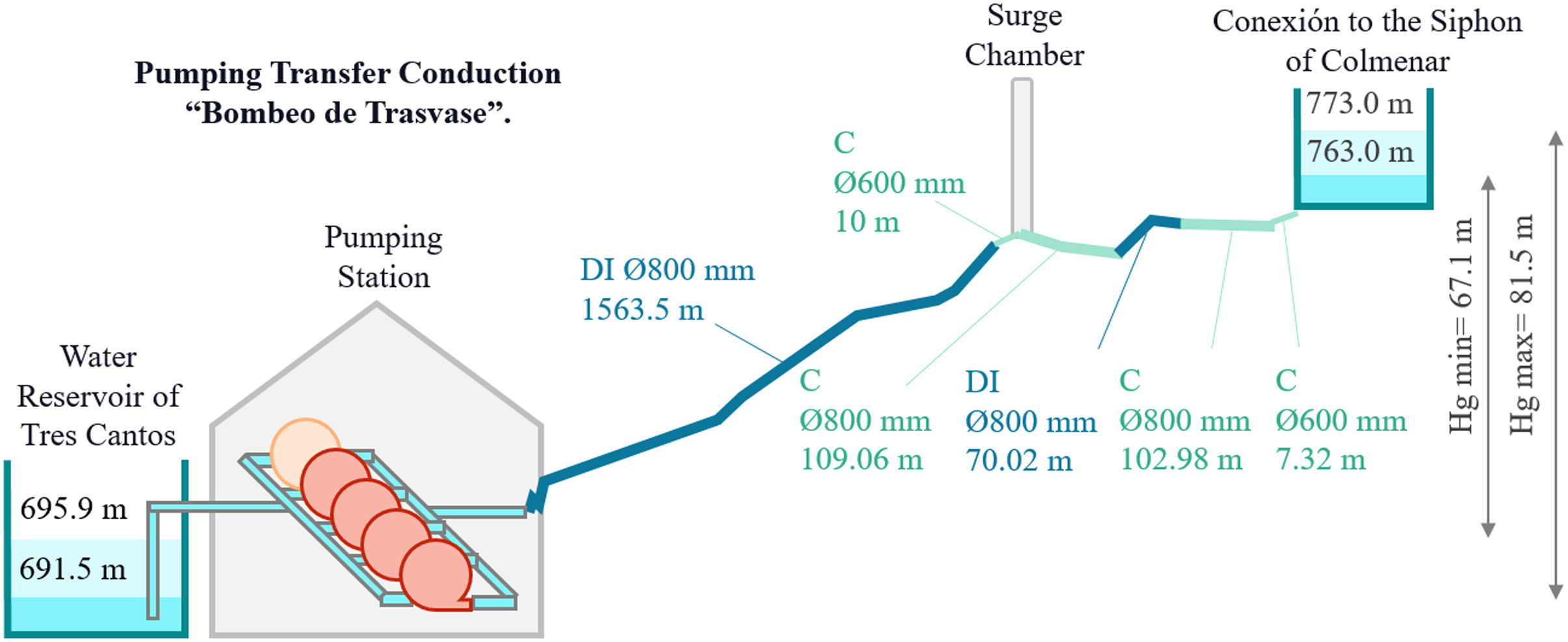
Technical details of the pumping transfer pipeline are specified in the project published by the Canal de Isabel II and are schematically summarized in Fig. 1.

Fig. 1. Schematic representation of the pumping transfer pipeline of Tres Cantos (Bombeo de Trasvase). DI, ductile function; H, concrete. 4 ( $+ 1$ ) reserved pumps.

As it can be seen from Fig. 1, the pipe consists of different materials. In marine blue, there are two different segments made of ductile iron (DI); light green shows the segments made of concrete (C). The pipe segments have different pipe diameters and lengths. The rugosity of the pipes was not specified in the project; in this article, however, it is assumed the typical values of Manning rugosity (Martín-Candilejo et al. 2022) for new pipes. This means that Manning rugosity for the ductile function is 0.011 and for concrete is 0.012.

As represented in the figure, the water level was variable at the initial point, the deposit of Tres Cantos (695.9 and –

691.5 m

), and also at the end point, the Siphon of Colmenar (773.0 and –

763.0 m

). For this reason, the geometric height difference

H_{g}

could vary from 67.1 to 81.5 m.

Depending on the geometric height difference (variable with changes on demand and incomes of water), the operational point will be swift and, therefore, so will the electrical consumption, which has a direct impact on the electricity cost.

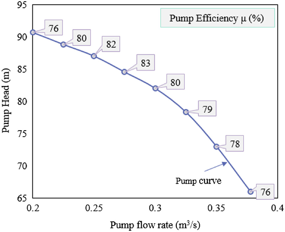
On the other hand, the project of rehabilitation of the deposit in the community of Tres Cantos also defines the pumps to be installed. This is a split-case hydraulic type of pump. Technical details of these pumps are shown in Fig. 2. The diameter of the pump impeller selected in the project is 495 mm.

Fig. 2. Split case hydraulic pump installed at the station (impeller diameter $φ 495 mm$ ), along with the pump efficiency at each point.

Results

Application of the Convex Hyperbola Method

To facilitate the reading of this article, at the end of the paper, the reader may find a list of the nomenclature used (Martín-Candilejo et al. 2021).

The aim of the optimization is to be able to determine how many pumps should be turned on and off to supply the water demand using the least amount of energy (and therefore at the lowest cost). This is achieved using the convex hyperbola method, which is a novel analytical method to find the optimal pump configuration for the operation of a pumping station (Martín-Candilejo et al. 2020). The method is mathematically deduced in this publication.

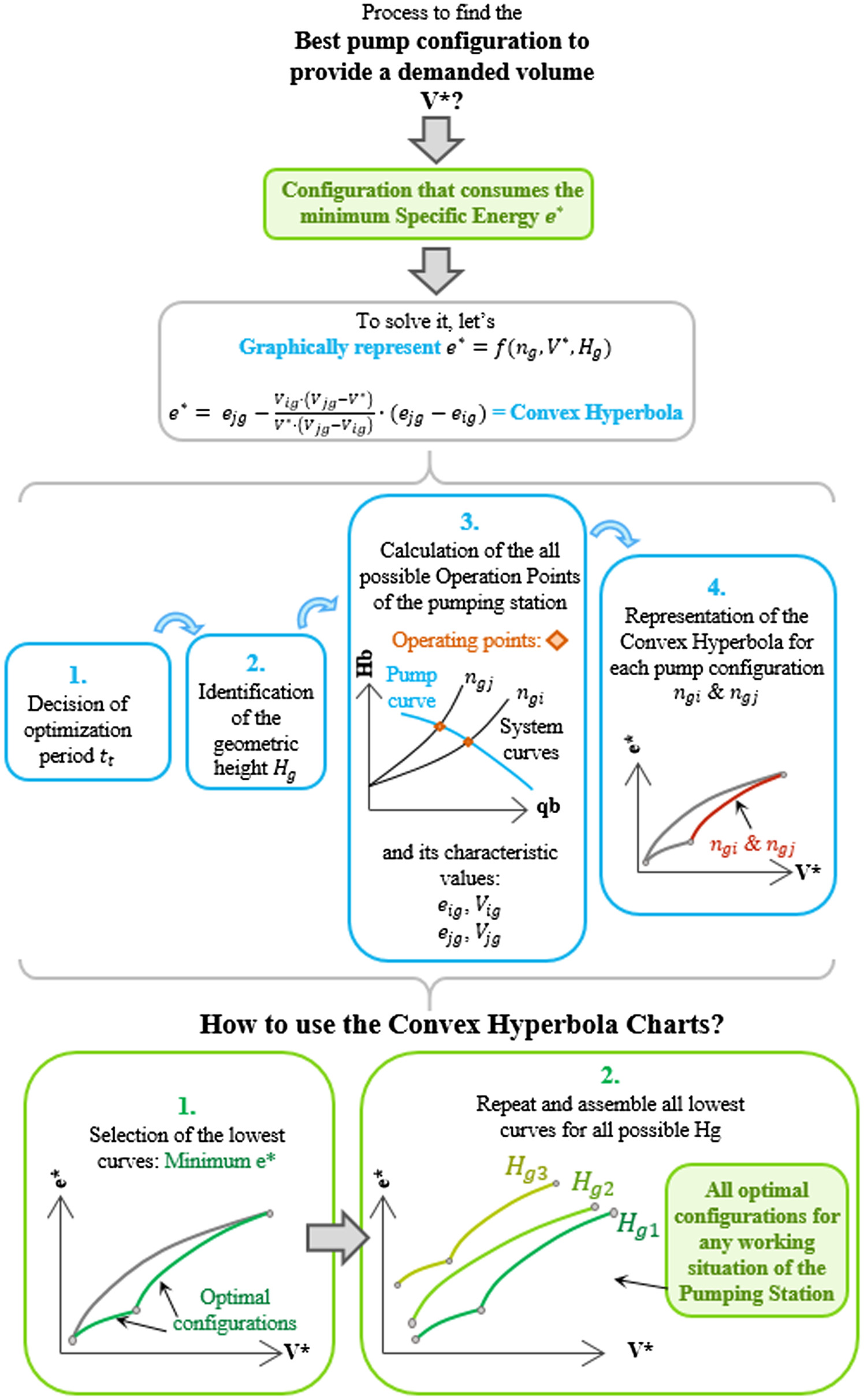
The convex hyperbola method uses the following steps:

1.

Determination of the optimization period

t_{t}

The convex hyperbola method requires a determined period of time

t_{t}

for the optimization. During this period of time

t_{t}

, a desired volume of water

V^{*}

is provided. The desired volume of water

V^{*}

is defined by the demand.

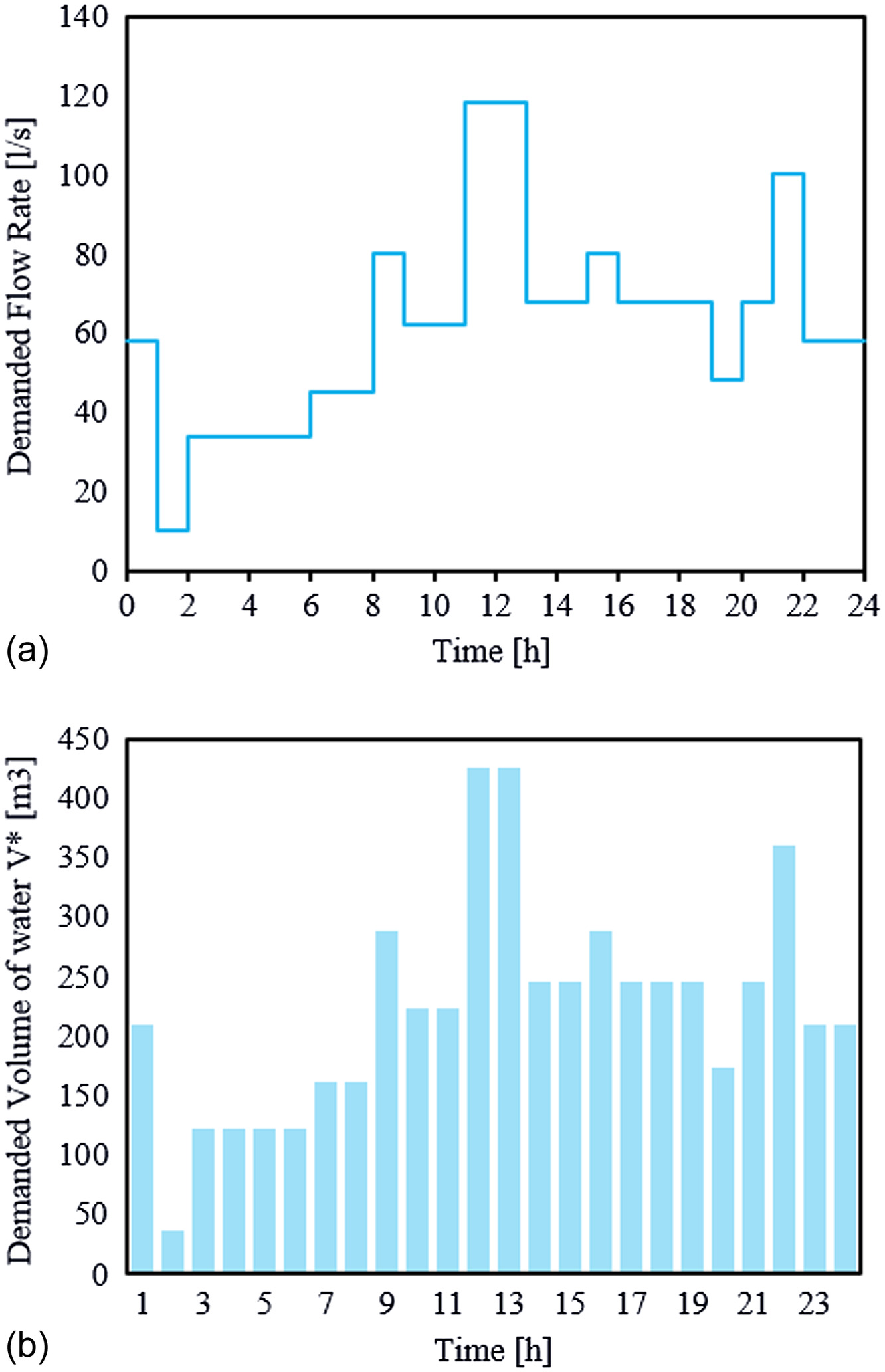
The project of rehabilitation of the deposit in the community of Tres Cantos established different demand scenarios. In all of them, it can be expected to have a different demand every 30 min to 3 h. Following the most immediate demand scenario, as represented in Fig. 3, the demand typically changes every hour, as shown; it is for this reason that the optimization time is fixed in

t_{t} = 1 h

. This means that knowing the desired volume of water every 1 h interval, as shown in Fig. 3(b), the method will be able to provide the best combination of operational pumps working during each interval of 1 h.

2.

Calculation of the characteristic values of the pumping station

In the geometric height difference, optimization of the operation of the pumping station depends on the pumping head required at the time, which also depends on the geometric height difference. Because, in the real case of the Bombeo de Trasvase, the geometric height difference (

H_{g}

) could vary from 67.1 to 81.5 m; thus, the optimization was carried out for 16 multiple situations with 16 different geometric height differences

(H_{g}) : 67.1

to 81.5 m.

Nevertheless, this article will show the optimization process for a geometric height of

H_{g} = 70 m

, and all other cases will proceed the same way.

3.

Method objective: Minimize the specific energy.

The method of optimization is based on calculating the station specific energy

e

, which is the amount of energy required to pump each cubic meter of water

m^{3}

. In this way

e = \frac{E}{V}

(1)

where

E

= energy; and

V

= volume of water.

The specific energy will change depending on the number of active pumps. The objective of the method consists of pumping at the lowest specific energy.

Using the formulas presented in Table 1, it is possible to calculate the specific energy the station would consume if the station was working with a fixed number of identical groups

n_{g}

during the entire time of the example’s optimization period

t_{t} = 1 h

. It is important to note that the convex hyperbola methodology requires that all pumps are identical—not only the model but also their working conditions (head and efficiency curves). Nevertheless, even though this represents a limitation for the method, it is common to find pumping stations that meet this requirement in which all groups are identical.

For example, if two pumps were working

n_{g} = 2

for the whole time

t_{t} = 1

h, then the station would be supplying a volume of water

V = V_{2 g}

while consuming

e_{2 g}

specific energy. The power

N

(kW) and the unit

power = N / Q

[the amount of power (kW) needed for each unit of flow rate (

m^{3} / s

)] are calculated as

Power : N = 9.81 \cdot Q \cdot h_{B} \cdot \frac{1}{μ_{B}} \cdot \frac{1}{μ_{M}}

(2)

Unit power : \frac{N}{Q} = 9.81 \cdot h_{B} \cdot \frac{1}{μ_{B}} \cdot \frac{1}{μ_{M}}

(3)

These values were calculated for the Tres Cantos real case, as shown in Table 2.

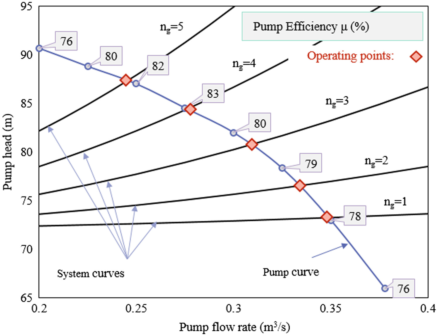
For calculating these values, the operational working points of the pumps were found, as shown in Fig. 4, using the pump curve (in blue) and the system curves (in black).

4.

Calculation of the convex hyperbolas

However, it has been proved (Martín-Candilejo et al. 2021) that, instead of working all of the time

t_{t}

with a fixed number or pumps, it is better to combine the number of active pumps to provide a certain volume of water. This means that, for example, instead of working for one full hour

t_{t} = 1 h

using two pumps all the time

n_{g} = 2

, it would be better to provide part of the desired volume of water using

n_{g} = 2

groups of pumps for some time, and then switching and pumping the rest of the volume with, e.g.,

n_{g} = 4

groups for the remaining time (or whatever other

n_{g}

the convex hyperbola method tells you to use).

In order to find the best group combinations to pump a desired volume of water

V^{*}

, as demonstrated by Martín-Candilejo et al. (2021), the convex hyperbolas need to be drawn, and they follow the next formulation

e^{*} = e_{j g} - \frac{V_{i g} \cdot (V_{j g} - V^{*})}{V^{*} \cdot (V_{j g} - V_{i g})} \cdot (e_{j g} - e_{i g})

(4)

t_{i g}^{*} = \frac{V^{*} \cdot t_{t}}{V_{i g}} \cdot \frac{(e^{*} - e_{g})}{(e_{i g} - e_{j g})}

(5)

where

e_{j g}

and

e_{i g}

= specific energy using

n_{g} = j

and

n_{g} = i

, respectively, for the whole time

t_{t}

;

V_{j g}

and

V_{i g}

= volume of water provided using

n_{g} = j

and

n_{g} = i

, respectively, for the whole time

t_{t}

; and

V^{*}

= desired volume of water; it is given working

n_{g} = j

for some time and then switching to

n_{g} = I

for the rest of the time;

e^{*}

= specific energy that would be consumed to provide

V^{*}

;

t_{i g}

and

t_{j g}

= portions of the optimization time

t_{t}

in which the system would be working with either

n_{g} = i

or

n_{g} = j

, respectively; and

t_{i g} + t_{j g} = t_{t}

.

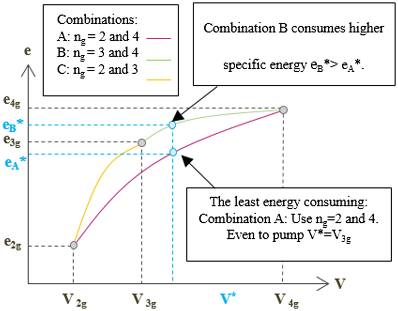
These curves express the following: Given a Group Combination A (see the pink curve in Fig. 5), for example,

n_{g} = 2

and 4 (pumping with

n_{g} = 2 g

and then switching to

n_{g} = 4

), a certain volume of water

V^{*}

(

V_{2 g} \leq V^{*} \leq V_{4 g}

) can be given consuming using

e^{*}

Combination A specific energy. Given a different Group Combination B (green curve in Fig. 5), for example,

n_{g} = 2

and

n_{g} = 3

, the same volume

V^{*}

may be given using

e^{*}

Combination B specific energy.

Because the specific energy

e^{*}

using Combination A is lower than the specific energy using Combination B, it means that, if you wish to provide

V^{*}

volume of water during

t_{t}

, it consumes less energy to use the Group Combination A:

n_{g} = 2

and 4, while Combination B:

n_{g} = 3

and 4 consumes more energy. Therefore, you should pump with

n_{g} = 2

for

t_{2 g}

time and then switch and pump with

n_{g} = 4

for

t_{4 g}

, this being the remaining time of

t_{t}

. This is how the convex hyperbola method tells you which is the best group combination to work with. The whole methodology is summarized in the flow chart in Fig. 6.

Even though the convex hyperbola methodology is not based on iterative process but on an analytical mathematical deduction of the function

e - V

(specific energy–volume provided), here is a description of the optimization process in the usual terms:

a.

Objective function: Minimization of the specific energy

e^{*}

;

b.

Decision variables: Geometric height

H g

and demanded volume

V^{*}

;

c.

Results after the optimization: The most optimal pump combination to provide a volume of water

V^{*}

in a period of time; and

d.

Constraints.

(1)

All pumps are identical; and

(2)

Demanded volume and geometric height need to be estimated in advance; therefore, the method works best when the demand is known or programmed.

e.

Advantages: The graphical representation of the convex hyperbola allows a general visualization of all possible pumping situations, so the same chart can be used in all operating cases, and provides a quick understanding of all solutions.

Fig. 3. Estimated demand for Tres Cantos: (a) estimated demand flow rate; and (b) estimated demand volume of water $V^{*}$ .

Table 1. Characteristic values of the pumping station. The station is pumping the whole time

t_{t}

using

n_{g}

Group number	Pump’s flow rate	Pumping head	Pump efficiency	Station flow rate	Station power	Station unit power	Station $volume$ ^a	Station specific energy
$n_{g}$	$q_{B}$	$h_{B} = H$	$μ_{B}$	$Q$	$N$	$N / Q$	$V$	$e$
$n_{g}$	From pump and system curve, obtained from the operational point			$Q = q_{B} \cdot n_{g}$	Eq. (2)	Eq. (3)	$V = Q \cdot t_{t}$	$e = \frac{N / Q}{3600}$
$1_{g}$	$q_{B 1 g}$	$h_{B 1 g} = H_{1 g}$	$μ_{B 1 g}$	$Q_{1 g}$	$N_{1 g}$	$N_{1 g} / Q_{1 g}$	$V_{1 g}$	$e_{1 g} = \frac{N_{1 g} / Q_{1 g}}{3600}$
—
$n_{g}$	$q_{B n g}$	$h_{B n g} = H_{n g}$	$μ_{B n g}$	$Q_{n g}$	$N_{n g}$	$N_{n g} / Q_{n g}$	$V_{n g}$	$e_{n g} = \frac{N_{n g} / Q_{n g}}{3600}$

a

Represents one group.

Table 2. Specific energy calculation in Bombeo de Trasvase

$n g$	$q b$ ( $m^{3} / s$ )	$μ B$ (%)	$h b$ (m)	$Q$ ( $m^{3} / s$ )	$N$ (kW)	$N / Q$	$V$ ( $m^{3}$ )	$e$ ( $KWh / m^{3}$ )
1	0.350	78.0	73.2	0.4	343	980	1,260	0.272
2	0.334	78.7	76.5	0.7	678	1,015	2,404	0.282
3	0.310	79.7	80.8	0.9	982	1,058	3,342	0.294
4	0.276	83.0	84.4	1.1	1,172	1,062	3,974	0.295
5	0.246	81.5	87.4	12	1,377	1,119	4,428	0.311

Fig. 4. Operating point of the pipeline when the height difference is $H_{g} = 70 m$ . In black, the pipeline curves for each number of groups ng activated. In blue, the pump curve. In the gray boxes, the values of the pump efficiency (in percentage). In orange, the operating points for each number of group situation.

Fig. 6. Summarization of the convex hyperbolas’ methodology.

The Convex Hyperbola Charts

Therefore, to follow the convex hyperbola method, it is necessary to draw the convex hyperbolas of all possible group combinations. Considering that the transfer pipeline of Tres Cantos has four (

+ 1

reserved) pumps, which makes up to 10 possible group combinations. These are shown in the first three columns of Table 3.

Table 3. Starting and ending points of the convex hyperbolas for

H_{g} = 70 m

Name of the combination	Number of pumps		Volume ( $m^{3}$ )		Specific energy ( $KWh / m^{3}$ )
Name of the combination	Starting with $n_{i}$	Then switch to $n_{j}$	$V_{i g}$	$V_{j g}$	$e_{i g}$	$e_{j g}$
A	1	2	1,260	2,404.8	0.272	0.282
B	1	3	1,260	3,342.6	0.272	0.294
C	1	4	1,260	3,974.4	0.272	0.295
D	1	5	1,260	4,428	0.272	0.311
E	2	3	2,404.8	3,342.6	0.282	0.294
F	2	4	2,404.8	3,974.4	0.282	0.295
G	2	5	2,404.8	4,428	0.282	0.311
H	3	4	3,342.6	3,974.4	0.294	0.295
I	3	5	3,342.6	4,428	0.294	0.311
J	4	5	3,9744	4,428	0.295	0.311

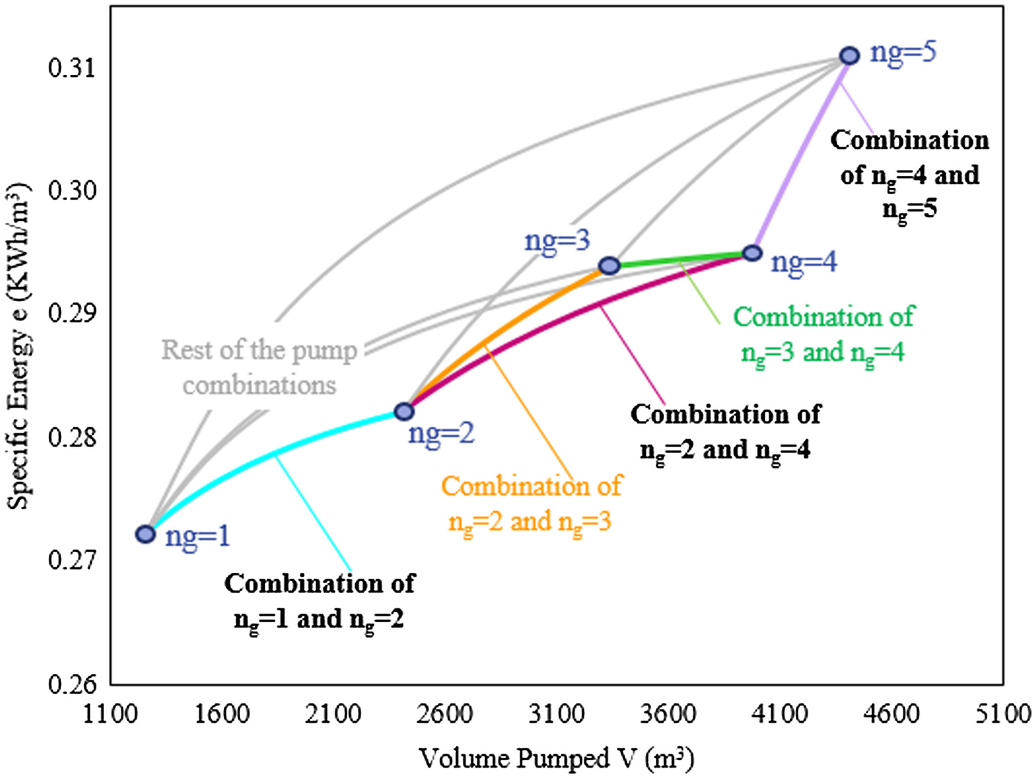
For all of these combinations, using Eq. (4) and the values of columns 4–7 of Table 3, the convex hyperbolas where drawn. The resulting curves can be seen in Fig. 7, which is interpreted as follows.

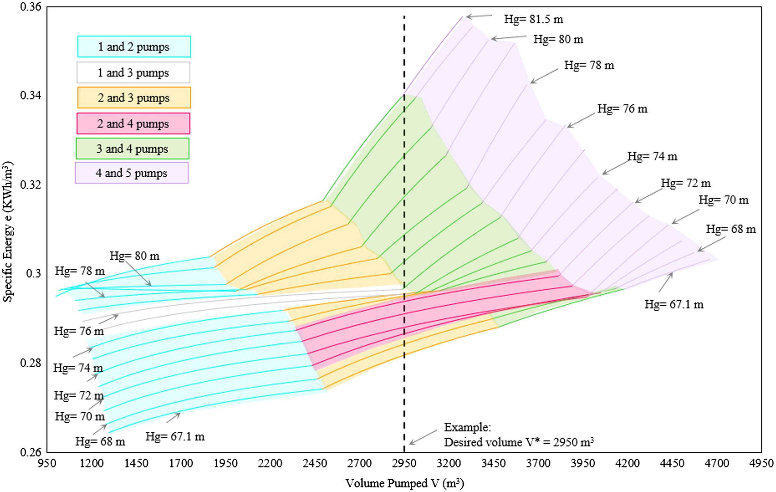
Fig. 7. Convex hyperbolas for $H_{g} = 70 m$ . In light blue, pink, and purple, the least-energy-consuming combinations of pumps for any desired volume of water. In orange, the combination of two and three pumps; in green, the combination of three and four pumps. Orange and green curves are higher than the curves of two and four pumps; therefore, either are a less preferable option for the operation of the pumping station.

When the transfer pipeline of Tres Cantos has a geometric height difference of

70 m

, and it is working for

t_{t} = 1 h

, if a volume of water

V^{*}

is desired, then it is best to work with the pump combinations, as indicated in Table 4.

Table 4. Best pump combinations for

H_{g} = 70 m

Volume $V^{*}$ ( $m^{3}$ )		Pump combination		In the chart
When a desired volume of water $V^{*}$ between $V_{i g}$ and $V_{j g}$ is wished		Then it is best to use the following pump combination		Color of the indicative curve in Fig. 7
$V_{i g}$	$V_{j g}$	Start with $n_{g i}$	Then switch to $n_{g j}$	Color of the indicative curve in Fig. 7
1,260	2,404.8	1	2	Light blue
2,404.8	3,974.4	2	4	Pink
3,974.4	4,428	4	5	Purple

The most relevant curves of the previous Fig. 7 are those located at the lowest part of the graph, since those indicate the combination of pumps that consume the minimum

e

, which is the minimum energy.

The distribution of pump combinations of this case study has turned out to be unexpected: When the system is working with this particular geometric height difference (70 m), there is no need to turn on only three pumps at any time. There is a “jump” that skips operating with only three pumps at the time. Any desired volume can be given at the lowest energy cost using either one and two pumps, two and four pumps, or even four and five pumps.

As shown in Fig. 4, it is possible to find the explanation for this phenomenon: When working with four groups, the pump efficiency is close to

μ_{B 4 g} \approx 83 %

, which is considerably higher than the pump efficiency given for three groups

μ_{B 3 g} \approx 79.7 %

. This makes working with

n_{g} = 4

less energetically consuming than

n_{g} = 3

. On the other hand, when working with

n_{g} = 2

, the pump efficiency

μ_{B 2 g} \approx 78.7 %

does not differ much from the previous

μ_{B 3 g}

. This makes working with

n_{g} = 2

a better option than

n_{g} = 3

, regardless of the 1% increase in the efficiency.

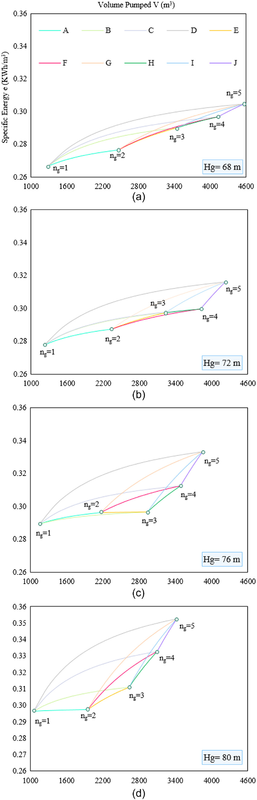
As explained at the beginning of the methodology of this paper, the geometric height difference of the transfer pipeline of Tres Cantos can vary from 67.1 to 81.5 m; therefore, the operational working points change as well as the specific energy consumed. In the previous sections, it was demonstrated how optimization is carried out when the geometric height difference is 70 m. Nevertheless, the convex hyperbola optimization method has also been carried out for all the geometric height differences: 67.1 to 81.5 m. Some of the resulting convex hyperbolas curves can be seen in Fig. 8.

Fig. 8. Convex hyperbolas for different $H_{g}$ : (a) $H_{g} = 68 m$ ; (b) $H_{g} = 72 m$ ; (c) $H_{g} = 76 m$ ; and (d) $H_{g} = 80 m$ . The legend of the figures is detailed in the first three columns of Table 3.

It is worth noting that some of the cases shown in the previous figures are much more predictable than the example case of

H_{g} = 70 m

. For instance, when

H_{g} = 80 m

, the lowest curves of the graph indicate that when

H_{g} = 80 m

there are no jumps in the expected consecution of working groups. Nevertheless, it is not always the case: When

H_{g} = 76 m

, it is best to skip operating with

n_{g} = 2

in any case, and pumping with

n_{g} = 1

and

n_{g} = 3

is a better option. This information is also shown in Table 5.

Table 5. Best pump combinations for

H_{g} = 80 m

Volume $V *$ ( $m^{3}$ )		Pump combination		In the chart
When a desired volume of water $V^{*}$ between $V_{i g}$ and $V_{j g}$ is wished		Then, it is best to use the following pump combination		Color of the indicative curve in Fig. 8
$V_{i g}$	$V_{j g}$	Start with $n_{g i}$	Then switch to $n_{g j}$	Color of the indicative curve in Fig. 8
1,051.2	1,951.2	1	2	Light blue
1,951.2	2,635.2	2	3	Orange
2,635.2	3,096	3	4	Green
3,096	3,420	4	5	Purple

As expected, if the geometric height difference increases, the pumping station will need more energy to move the water at higher heights and will do so pumping a smaller volume of water. That is exactly what these figures are showing: the curves get displaced toward the upper-left corner, which means higher specific energy and lower volumes.

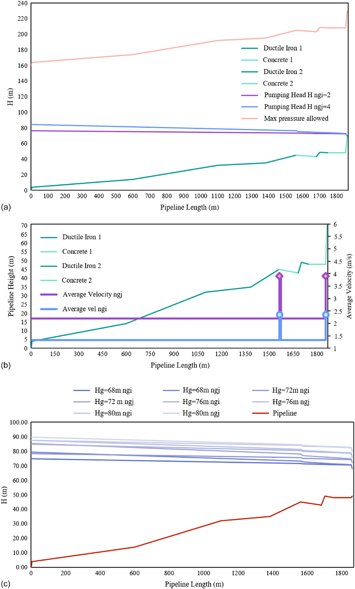
The hydraulic evaluation of the optimal solution for different geometric heights was also obtained. Following with the exemplification of the methodology for

H_{g} = 70 m

and a desired volume of

2,950 m^{3}

, the hydraulic state of the pumping station is calculated, as shown in Table 6, using the formulation shown previously in this paper and in Table 1. In addition, the hydraulic evaluation of pressure and water velocity along the pipeline was also calculated. There are two energy lines represented for each of the group configurations

n_{g i}

and

n_{g j}

, which, in the case of

H_{g} = 70 m

and

V = 2,950 m^{3}

, is

n_{g i} = 2

and

n_{g j} = 4

. This is shown in Table 7 and Fig. 9 for

H_{g} = 70 m

and Fig. 9 for

H_{g} = 68

, 72, 76, and 80 m.

Table 6. Hydraulic state of the pumping station.

H_{g} = 70 m

Group number	Time of each $n g$ working	Pump’s flow rate	Station flow rate	Pumping height	Pump efficiency	Volume pumped	Station specific energy	Station power	Station energy
$n g$	$t g$ (min)	$q b$ ( $m^{3} / s$ )	$Q t$ ( $m^{3} / s$ )	$h$ (m)	$μ_{B}$ (%)	$V$ ( $m^{3}$ )	$e$ ( $KWh / m^{3}$ )	$N$ (KW)	$E$ (KWh)
2	39.2	0.33	0.668	76.5	79%	1,569	0.188	678	26,553
4	20.8	0.28	1.104	84.4	83%	1,381	0.100	1,172	24,425
Best convex hyperbola	Total	Average	Average	—	—	Total	Total	Total	Total
F	60	0.314	0.819	—	—	2,950	0.288	1,850	50,978

Table 7. Hydraulic state of the pipeline.

H_{g} = 70 m

Pipeline location	Units	Pumping station	Ductile iron (part1)	Concrete (part1)		Ductile iron (part 2)	Concrete (part 2)		Conexión to the Siphon of Colmenar
Pipeline location	Units	PS	DI1	C1	C1	DI2	C2	C2	Conexión to the Siphon of Colmenar
Pipeline length	m	0	1,563.5	1,573.5	1,682.6	1,752.6	1,855.6	1,862.9	1,862.9
Pipeline relative height	m	0	45	44	43	48	68	49	70
While $n_{g} = 2$ pumps
Head	m	76.5	73.6	73.2	72.9	72.7	72.4	70.0	70.0
Average velocity	m		1.33	2.36	1.33	1.33	1.33	2.36
Pressure	m wc	76.5	28.6	29.2	29.9	24.7	4.4	21.0	0.0
While $n_{g} = 4$ pumps
Head	m	84.4	76.4	75.3	74.4	73.8	73.0	70.0	70.0
Average velocity	m		2.20	3.90	2.20	2.20	2.20	3.90
Pressure	m wc	84.4	31.4	31.3	31.4	25.8	5.0	21.0	0.0

Fig. 9. Hydraulic state of the pipeline when $H_{g} = 70 m$ and demanded volume in $t = 1 h$ is $V = 2,950 m^{3}$ . In this particular case, the best configuration is Hyperbola F: use $n_{g} = 2$ pumps; after 39.2 min switch to $n_{g} = 4$ pumps for 20.8 min (See Table 8): (a) When $n_{g} = 2$ , the pumping head and energy along the pipeline are represented in blue and in purple when $n_{g} = 4$ . The project document does not specify the nominal pressure of the pipes, since no manufacturer is specified; however, it does mention the nominal pressure of the valves as in $PN = 16 = 160 m$ wc. For reference, it was represented in orange the maximum pressure if all pipelines had PN16; (b) the velocity along the pipeline when $n_{g} = 2 ($ blue) and $n_{g} = 4$ (purple) pumps are working. The velocity shows an expected increase in the points of reduced diameter; and (c) pressure along the pipeline for a demanded volume of $V = 2,950 m^{3}$ and different height differences.

By assembling all of the lowest curves of the graphs, a general operational chart is obtained, which is shown in Fig. 10.

Fig. 10. Lowest convex hyperbolas compilation for all possible geometric heights in the Bombeo el Trasvase $Hg \in (67.1 - 81.5 m)$ with an interval of $t_{t} = 1 h$ . These curves indicate the best possible combination of pumps for any possible pumping situation. In blue, it shows the situations in which it is best to pump with one and two pumps; in white: one and three pumps (skipping the use of just two pumps); in orange: two and three pumps (as shown, this is not a stable combination that turns out to be not desirable for many different pumping head); in pink: two and four pumps; in green: three and four pumps; and in purple: four and five pumps. It can be seen that the regions shown in white and pink are quite large; therefore, there are many situations in which a jump in the number of pumps is recommended.

This figure assembles all the information required for the operation of the pumping station with an hourly regulation

t_{t} = 1 h

. It tells the operator the number of groups of pumps that should be turned on or off at any time.

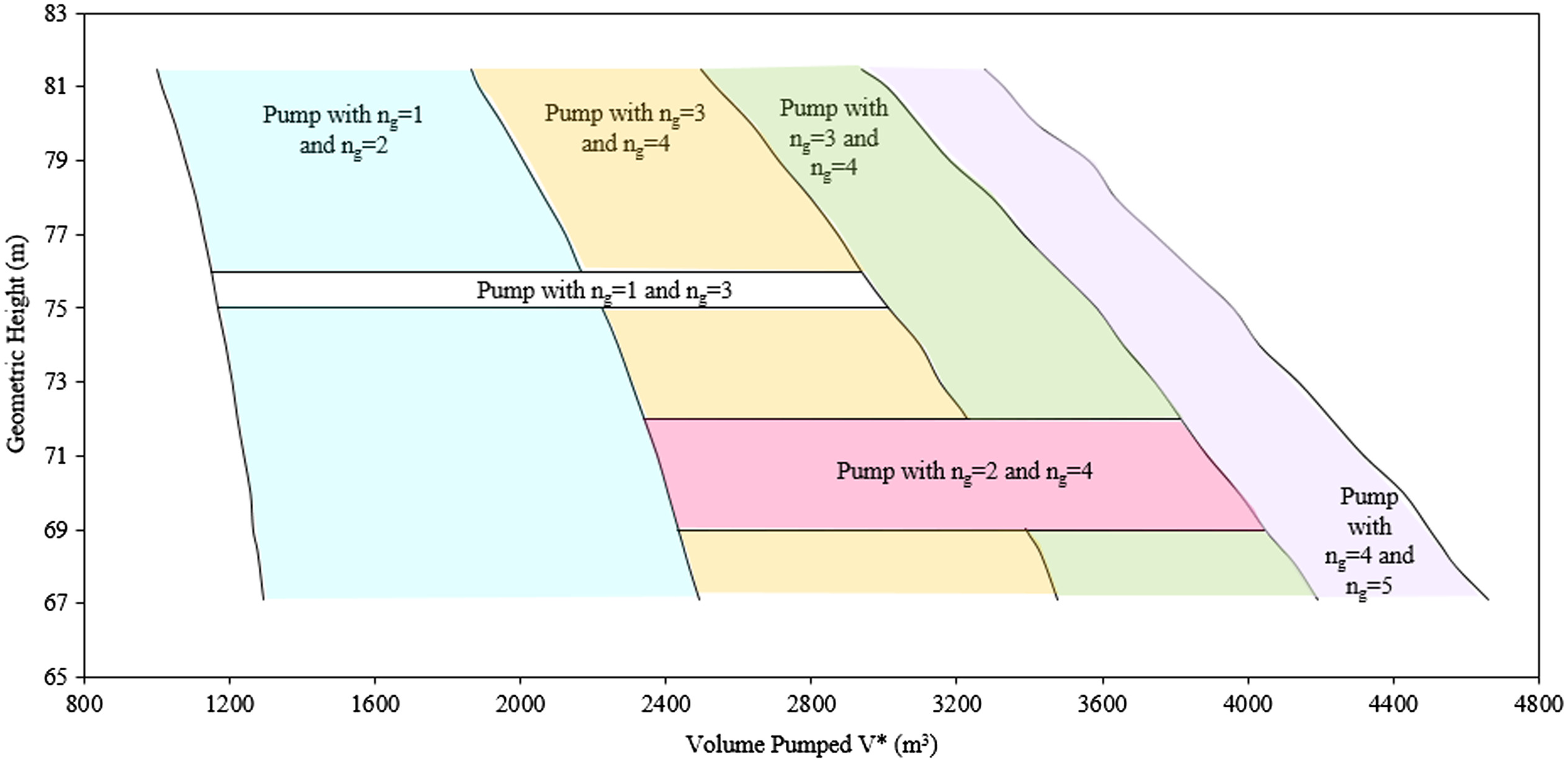
Fig. 11 shows a similar schematic representation of pumping combinations that should be used to pump a certain volume of water for

t_{t} = 1 h

, depending on the geometric height difference.

Fig. 11. Combination of the number of pumps for different geometric height difference, depending of the volume of water to pump during $t_{t} = 1 h$ .

For instance, if a volume of

1,450 m^{3}

was required in an hour, and the geometric height difference between deposits was

70 m

,

n_{g} = 1

should be used and then switched to

n_{g} = 2

, as the region marked in blue color indicates. If the geometric height difference was 76 m, however, use one pump and then switch to three pumps. For the situation in which a volume of

2,950 m^{3}

is required, as shown in Fig. 10, Table 8 shows the time that each number of pumps should be working. These values have been obtained with Eqs. (1)–(5). This is an interesting case since the combination of pumps varies depending on the geometric height difference.

1.

Calculation of the energy savings by using nonconsecutive number of pumps

It is also interesting to evaluate the energy savings that the convex hyperbola method offers when these jumps are detected. The logic procedure would be to increase consecutively the number of pumps along with the demand, activating or disactivating them one by one.

Nevertheless, as shown in the examples of this paper, it may be better to activate or disactivate more pumps in a nonconsecutive number, skipping a certain number of pumps, and therefore producing the so-called “jumps.” To illustrate how much energy savings can be obtained, let’s take, once again, the case in which a volume of

2,950 m^{3}

was required in

t_{t} = 1

h. In Fig. 10 and Table 8, it can be seen that, for the geometric height difference of 75–76 m, there was a jump in the combination of pumps, since the best combination is using

n_{g} = 1

and 3 for 75 m, as marked in white-gray; and

n_{g} = 2

and 4 for

H_{g} = 69 - 72 m

, as marked in pink. This can also be seen in Fig. 11. However, if these jump areas were ignored and went for the more predictable (but not optimal) configurations of the regions from behind, the nonoptimal configuration of pumps would tell the reader to work with

n_{g} = 2

and 3 pumps for the previous cases. The energy consumption when working with the optimal and nonoptimal configuration was calculated, as shown in Table 8. The table also shows the additional KWh that would be consumed in 1 h. The monetary cost of the energy was also estimated based on the average price of energy in Spain in November 2022, which is 0.3 €/KWh (which shows a rising tendency). The savings may seem small, but let’s remember that this is only for 1 h and that particular demand of volume of water. Considering, this is just a small representation of one of the many situations in which the water demand is not served using the optimal configurations; thus, the savings throughout the entire life of the pumping systems can become significant.

2.

Analysis of the convex hyperbolas

As explained, Fig. 10 summarizes all of the lowest convex hyperbolas that tell the operators the best pump combination. Fig. 11 shows the regions for the different configurations of pumps, depending on the demanded volume of water and the geometric height difference. The curves that mark the separation of these areas are equivalent to the pump curve when different number of groups are performing. The shape of the different regions of the configurations can be described as an “inclined trapezoidal stripe,” interrupted by those regions in which a jump in the pump combination is happening.

The irregularities in the border lines “inclined trapezoidal stripes” have much to do with the irregularities of the distribution of the pump efficiency in the pump curve. A homogenous distribution of the pump efficiency along the pump curve translates in a reduction of these irregularities and a reduction of the jumps. This effect of the distribution of the pump efficiency is also shown in Fig. 11 and the gaps inside. Future research to predict the shape of these curves is being considered.

Table 8. Comparison on the optimization

Geometric height	Optimization A: considering nonconsecutive number of pumps							Optimization B: consecutive number of pumps
$H g$	$n_{g i}$	$n_{g j}$	Jump in the number of pumps	$e^{*}$	$t_{g i}$	$t_{g j}$	$E$	$n_{g i}$	$n_{g j}$	$e^{*}$	$t_{g i}$	$t_{g j}$	$E$	Energy savings
(m)	(n° pumps)		Jump in the number of pumps	( $KWh / m^{3}$ )	(min)		(KWh)	(n° pumps)		( $KWh / m^{3}$ )	(min)		(KWh)	(KWh)
67.1	2	3		0.282	32	28	831	2	3	0.282	32	28	831
68	2	3		0.284	30	30	839	2	3	0.284	30	30	839
69	2	4	Jump	0.287	41	19	846	2	3	0.287	28	32	847	1.6
70	2	4	Jump	0.288	39	21	850	2	3	0.290	25	35	855	5.3
71	2	4	Jump	0.291	37	23	859	2	3	0.292	21	39	862	3.6
72	2	4	Jump	0.294	35	25	867	2	3	0.295	19	41	869	2.4
73	2	3		0.295	14	46	871	2	3	0.295	14	46	871
74	2	3		0.296	11	49	872	2	3	0.296	11	49	872
75	1	3	Jump	0.296	2	58	872	2	3	0.296	5	55	872	0.1
76	3	4		0.297	59	1	876	3	4	0.297	59	1	876
77	3	4		0.303	51	9	893	3	4	0.303	51	9	893
78	3	4		0.309	42	18	911	3	4	0.309	42	18	911
79	3	4		0.317	30	30	936	3	4	0.317	30	30	936
80	3	4		0.327	19	41	964	3	4	0.327	19	41	964
81	3	4		0.337	8	52	993	3	4	0.337	8	52	993
81.5	4	5		0.341	58	2	1,005	4	5	0.341	58	2	1,005

Discussion

This research demonstrates the practical applicability of a theorical methodology to optimize the operation of a pumping station in a water supply system: the convex hyperbola charts. A step-by-step application is shown.

Moreover, it is analyzed how the distribution of the pump efficiency can affect pump selection. Sometimes pumps show a distribution of their efficiency that is not equally spaced along the pump curve. This can translate into a poor operation point, which should be skipped for a less-energy-consuming configuration. Traditionally, pumps are turned on and off in a consecutive manner (e.g., one by one). Nevertheless, depending on the characteristics of the pump, this consecutive manner might not be the most optimal strategy. This phenomenon is studied in the paper, proving that skipping a certain number of pumps can be a better option.

On the other hand, the pumping station aims to provide water with a certain flow rate at a certain height. The pumping head has a direct effect on the determination of the operation point. Once again, depending on the characteristics of the pump, the operation points might drastically change the energy consumption, and it may be better to skip certain configurations turning on/off more pumps and not necessarily in a consecutive manner. This can change the strategy of the operation. Therefore, the impact of the variability of the pumping head is studied in this work.

More specifically, the aim of this work was to determine the number of pumps that should be working at any moment during the operation of the pumping station of Tres Cantos, in Madrid, Spain. The aim is to provide the desired volume of water whilst consuming the least amount of energy. Such optimization has been made using the convex hyperbola charts, to put the effectivity of the method to test.

The charts and method take their name from the shape of the curves’ specific energy– volume. The specific energy

e^{*}

is the amount of energy consumed by the station per volume. The pumping station should pump the desired volume of water

V^{*}

using the least-specific energy

e^{*}

. The shape of the curves

e^{*} - V^{*}

turns out to be a convex hyperbola.

The specific energy

e^{*} - V^{*}

was plotted for the station of Tres Cantos, considering the particular pump curve of the station as well as the different height levels of the deposits in the installation. Therefore, many different pumping situations have been studied, with charts plotted for each of them.

With each of these charts, the best combination of pumps to turn on can be known in each pumping situation. Already, the elaboration of the convex hyperbola charts has proven to be a straightforward methodology with easy applicability in real cases. The effectivity of the method to find the best pump combination during different moments of the operation has been proven as well. It is not only an effective method, but, most importantly, it is based on an analytical deduction; for this reason, the optimization is not an approximation; on the contrary, it is exact. It is important to realize that the method is exact when the operators know in advance the volume of water to be delivered as well as the geometric height. Therefore, the method is especially useful in those cases in which the demand is known or programmed (such as in some agricultural installations or industrial processes) or, at least, in those cases in which there is a solid knowledge on how demand typically fluctuates. Nevertheless, for those cases in which this ideal situation is not the reality, the graphical representation is still useful for determining the best pump combination; notably, with Fig. 9, the operator is capable to take into consideration a rough estimation of the geometric height, even if it constantly changes, since wide regions of geometric heights are represented in the graph in different colored areas.

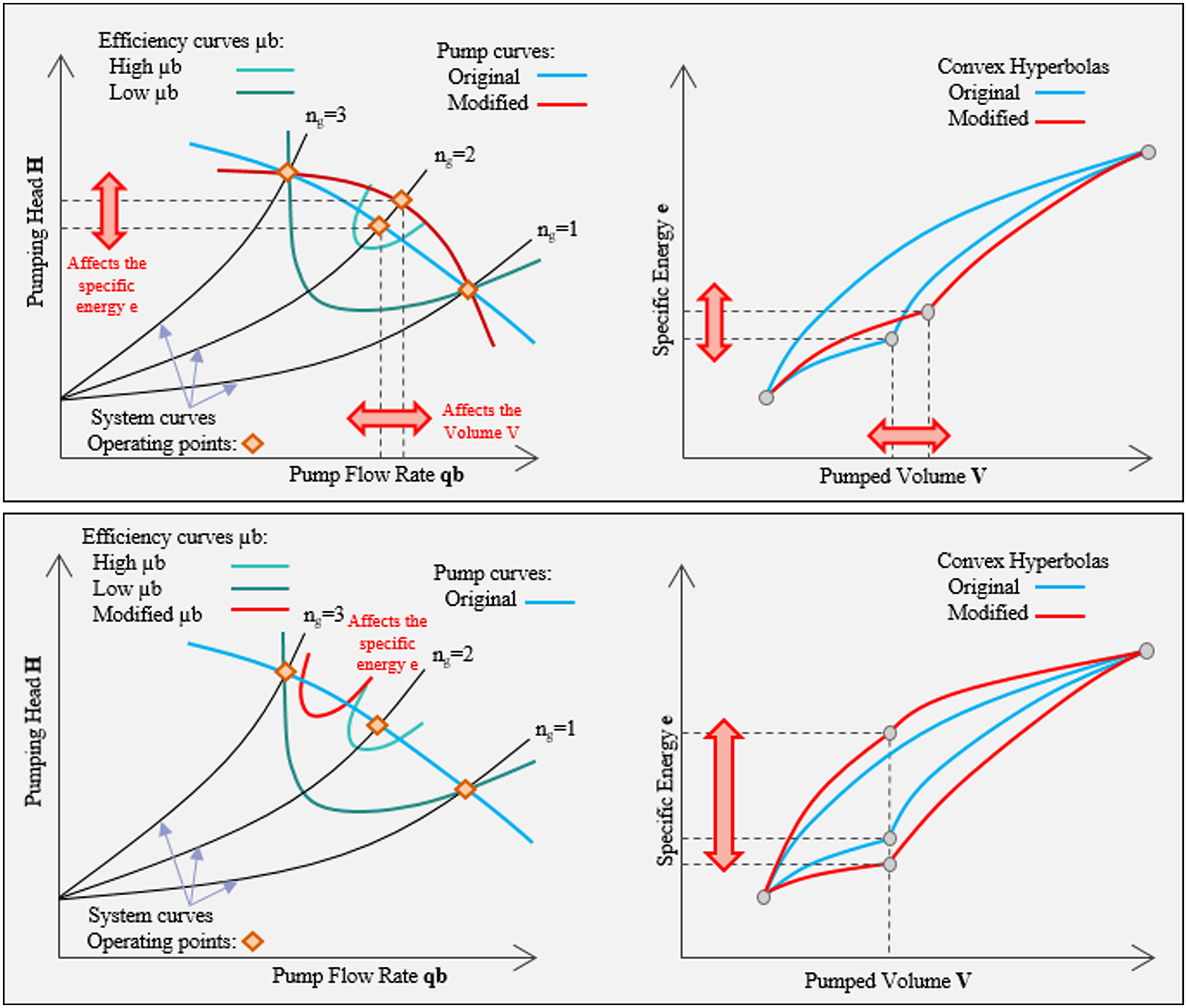
Moreover, the results of the distribution of the convex hyperbolas of this case study show an unexpected aspect: Many times, it is better to work with a nonconsecutive number of pumps. This could mean, for example, working with one pump at the beginning and then switching and activating three pumps or work with two pumps and then switching to four pumps. These jumps depend on the particular characteristics of the pump, e.g., the efficiency distribution or the shape of the curve itself. Therefore, they cannot be generalized. How the pump efficiency is distributed over the pumping curve of the particular model of commercial pump has a direct impact on the operation configuration and on which groups would be better to skip. Fig. 12 schematically represents how the variation of the mentioned can later affect the shape of the convex hyperbolas and, therefore, the selection of pump combinations. Future research to be able to predict the shape of the convex hyperbolas depending on the pump curve and its efficiency is being studied. This methodology assumes that the installation is already built (and that the pump has already been chosen to best fit the expected operational points).

Fig. 12. Schematic representation of how the shape of the pump curve or the distribution of the pump efficiency affects the shape of the convex hyperbolas; therefore, it may affect the selection of the most optimal combination of pumps.

The making of these charts only required the use of a calculation sheet, only once; it is also a permanent resource that can be used at any time during the operation. Therefore, it is completely inexpensive in both the material and the computational aspect. No heavy complex algorithm was required; on the contrary, it was simply done with Excel. Therefore, the methodology can be exported to areas with low resources. The methodology tested here comes from the mathematical deduction of the specific energy used and not from any iterative process, which is the current trend. Further, the graphical representation of the optimization solution is helpful for a quick understanding and direct usage by operators.

Finally, it is important to answer what kind of water drives this method can be applied to (pipelines, meshed networks, etc.) and in which cases is it best to apply the convex hyperbola methodology or other classical heuristic algorithms. To answer these questions, it is important to remember what the convex hyperbola methodology is based on.

The convex hyperbolas show the specific energy that would be consumed when a certain volume of water is provided, for all pump combinations. To elaborate on these curves, the engineer needs to know how much specific energy would be consumed if

n_{g}

of pumps were pumping the whole optimization period

t

. This is calculated from the operating points, given by crossing of the pump curve and the system’s curve. The system curve is elaborated based on the characteristics of the water drive, regardless of whether it is a pipeline or a network. Nevertheless, the system’s curve of a single pipeline is much easier to calculate than the curve of a complex network, where many operating points can be expected. Therefore, the method can be applied to any water drive; the difficulty increases, however, with the complexity of the water drive. This method is a quick, affordable, and easy alternative when speaking of simpler water drives, with limited expected operation points, since overall visualization of all possible operating situations can be achieved. However, for meshed networks, it is better to use the other classical heuristic algorithms, which are designed to carry out heavy iterative processes.

The effectivity of the convex hyperbola charts methodology for the optimization of the operation of a pumping station has been proved. It was shown how, depending on the pumping circumstances, it may be better to avoid working with a consecutive number of pumps. An example on the use of a powerful and simple tool to be more energetically mindful in the operation of water supply systems was presented.

Notation

The following symbols are used in this paper:

$E$: energy;
$e$: specific energy;
$e^{*}$: specific energy to provide $V^{*}$ during $t_{t}$ ;
$H_{g}$: geometric height difference;
$N$: power;
$n_{g}$: number of groups of pumps working at the same time;
$t_{t}$: period of time for the optimization. A specific volume of water $V^{*}$ is demanded during that time. Therefore, $t_{t}$ needs to be adjusted to the typical interval duration of changes in the demand;
$t_{i g}$ and $t_{j g}$: portions of the optimization time $t_{t}$ in which the system would be working with either $n_{g} = i$ or $n_{g} = j$ , respectively; $t_{i g} + t_{j g} = t_{t}$ ;
$V$: volume of water;
$V^{*}$: demanded volume of water during the optimization time $t_{t}$ ;
$V_{j g}$ and $V_{i g}$: volume of water provided using $n_{g} = j$ and $n_{g} = i$ , respectively, for the whole time $t_{t}$ ;
$μ_{B}$: pump efficiency; and
$μ_{M}$: engine efficiency.

Data Availability Statement

All data, models, or code that support the findings of this study are available from the corresponding author upon reasonable request.

Acknowledgments

This work was funded by the Fundación Carlos Gonzalez Cruz with the grant Ayudas para el Fomento de la Investigación.

References

Abiodun, F. T., and F. S. Ismail. 2013. “Pump scheduling optimization model for water supply system using AWGA.” In Proc., IEEE Symp. on Computers and Informatics, ISCI 2013, 12–17. New York: IEEE. https://doi.org/10.1109/ISCI.2013.6612367.

Google Scholar

Ahmad, S., H. Jia, Z. Chen, Q. Li, and C. Xu. 2020. “Water-energy nexus and energy efficiency: A systematic analysis of urban water systems.” Renewable Sustainable Energy Rev. 134 (Dec): 110381. https://doi.org/10.1016/j.rser.2020.110381.

Google Scholar

Alberto Gaitón Vicente. 2016. Proyecto Constructivo de Rehabilitación Del Depósito de Tres Cantos. Madrid, Spain: Canal Isabel II. Gestión.

Google Scholar

Andrés, S., M. Dentz, and L. Cueto-Felgueroso. 2021. “Multirate mass transfer approach for double-porosity poroelasticity in fractured media.” Water Resour. Res. 57 (8): e2021WR029804. https://doi.org/10.1029/2021WR029804.

Google Scholar

Andrés, S., D. Santillán, J. Carlos Mosquera, and L. Cueto-Felgueroso. 2019. “Thermo-poroelastic analysis of induced seismicity at the Basel enhanced geothermal system.” Sustainability 11 (24): 6904. https://doi.org/10.3390/su11246904.

Google Scholar

Ayyagari, K. S., S. Wang, N. Gatsis, A. F. Taha, and M. Giacomoni. 2021. “Energy-efficient optimal water flow considering pump efficiency.” In Proc., 2021 IEEE Madrid PowerTech. New York: IEEE. https://doi.org/10.1109/PowerTech46648.2021.9494803.

Google Scholar

Bejarano, M. D., A. Sordo-Ward, I. Gabriel-Martin, and L. Garrote. 2019. “Tradeoff between economic and environmental costs and benefits of hydropower production at run-of-river-diversion schemes under different environmental flows scenarios.” J. Hydrol. 572 (May): 790–804. https://doi.org/10.1016/j.jhydrol.2019.03.048.

Google Scholar

Bene, J. G., I. Selek, and C. Hös. 2009. “Neutral search technique for short-term pump schedule optimization.” J. Water Resour. Plann. Manage. 136 (1): 133–137. https://doi.org/10.1061/(ASCE)0733-9496(2010)136:1(133).

Google Scholar

Bolognesi, A., C. Bragalli, C. Lenzi, and S. Artina. 2014. “Energy efficiency optimization in water distribution systems.” Procedia Eng. 70 (January): 181–190. https://doi.org/10.1016/j.proeng.2014.02.021.

Google Scholar

Brentan, B., G. Meirelles, E. Luvizotto Jr., and J. Izquierdo. 2018. “Joint operation of pressure-reducing valves and pumps for improving the efficiency of water distribution systems.” J. Water Resour. Plann. Manage. 144 (9): 04018055. https://doi.org/10.1061/(ASCE)WR.1943-5452.0000974.

Google Scholar

Briceño-León, C. X., P. L. Iglesias-Rey, F. J. Martinez-Solano, D. Mora-Melia, and V. S. Fuertes-Miquel. 2021. “Use of fixed and variable speed pumps in water distribution networks with different control strategies.” Water 13 (4): 479. https://doi.org/10.3390/w13040479.

Google Scholar

Campana, P. E., P. Lastanao, S. Zainali, J. Zhang, T. Landelius, and F. Melton. 2022. “Towards an operational irrigation management system for Sweden with a water–food–energy nexus perspective.” Agric. Water Manage. 271 (Sep): 107734. https://doi.org/10.1016/j.agwat.2022.107734.

Google Scholar

Campana, P. E., H. Li, J. Zhang, R. Zhang, J. Liu, and J. Yan. 2015. “Economic optimization of photovoltaic water pumping systems for irrigation.” Energy Convers. Manage. 95 (May): 32–41. https://doi.org/10.1016/j.enconman.2015.01.066.

Google Scholar

Campana, P. E., J. Zhang, T. Yao, S. Andersson, T. Landelius, F. Melton, and J. Yan. 2018. “Managing agricultural drought in Sweden using a novel spatially-explicit model from the perspective of water-food-energy nexus.” J. Cleaner Prod. 197 (Oct): 1382–1393. https://doi.org/10.1016/j.jclepro.2018.06.096.

Google Scholar

Cassiolato, G., E. P. Carvalho, J. A. Caballero, and M. A. Ravagnani. 2020. “Optimization of water distribution networks using a deterministic approach.” Eng. Optim. 53 (1): 107–124. https://doi.org/10.1080/0305215X.2019.1702980.

Google Scholar

CEN (European Committee for Standardization). 2014. Energy climate policy framework EU 2020–2030. Brussels, Belgium: CEN.

Google Scholar

Chaban, A., M. Lis, and A. Szafraniec. 2022. “Voltage stabilisation of a drive system including a power transformer and asynchronous and synchronous motors of susceptible motion transmission.” Energies 15 (3): 811. https://doi.org/10.3390/en15030811.

Google Scholar

Chen, W., T. Tao, A. Zhou, L. Zhang, L. Liao, X. Wu, K. Yang, C. Li, T. C. Zhang, and Z. Li. 2021. “Genetic optimization toward operation of water intake-supply pump stations system.” J. Cleaner Prod. 279 (Jan): 123573. https://doi.org/10.1016/j.jclepro.2020.123573.

Google Scholar

Cimorelli, L., C. Covelli, B. Molino, and D. Pianese. 2020. “Optimal regulation of pumping station in water distribution networks using constant and variable speed pumps: A technical and economical comparison.” Energies 13 (10): 2530. https://doi.org/10.3390/en13102530.

Google Scholar

Cojanu, V., and E. Helerea. 2021. “Considerations on the efficient functioning of the urban water pumping stations.” IOP Conf. Ser.: Mater. Sci. Eng. 1138 (1): 012017. https://doi.org/10.1088/1757-899X/1138/1/012017.

Google Scholar

Dadar, S., B. Đurin, E. Alamatian, and L. Plantak. 2021. “Impact of the pumping regime on electricity cost savings in urban water supply system.” Water 13 (9): 1141. https://doi.org/10.3390/w13091141.

Google Scholar

EPA. 2008. Ensuring a sustainable future: An energy management guidebook for wastewater and water utilities. Washington, DC: EPA.

Google Scholar

Esen, H., and E. Turgut. 2015. “Optimization of operating parameters of a ground coupled heat pump system by Taguchi method.” Energy Build. 107 (Nov): 329–334. https://doi.org/10.1016/j.enbuild.2015.08.042.

Google Scholar

Ezaz, G. T., K. Zhang, X. Li, M. H. Shalehy, M. A. Hossain, and L. Liu. 2022. “Spatiotemporal changes of precipitation extremes in Bangladesh during 1987–2017 and their connections with climate changes, climate oscillations, and monsoon dynamics.” Global Planet. Change 208 (Jan): 103712. https://doi.org/10.1016/j.gloplacha.2021.103712.

Google Scholar

Fecarotta, O., A. Carravetta, M. Cristina Morani, and R. Padulano. 2018. “Optimal pump scheduling for urban drainage under variable flow conditions.” Resources 7 (4): 73. https://doi.org/10.3390/resources7040073.

Google Scholar

Filipe, J., R. J. Bessa, M. Reis, R. Alves, and P. Póvoa. 2019. “Data-driven predictive energy optimization in a wastewater pumping station.” Appl. Energy 252 (Oct): 113423. https://doi.org/10.1016/j.apenergy.2019.113423.

Google Scholar

Garrote, L. 2021. “Water resources management models for policy assessment.” Water 13 (8): 1063. https://doi.org/10.3390/w13081063.

Google Scholar

Iglesias, A., and L. Garrote. 2015. “Adaptation strategies for agricultural water management under climate change in Europe.” Agric. Water Manage. 155 (June): 113–124. https://doi.org/10.1016/j.agwat.2015.03.014.

Google Scholar

Iglesias, A., L. Garrote, A. Diz, J. Schlickenrieder, and M. Moneo. 2013. “Water and people: Assessing policy priorities for climate change adaptation in the Mediterranean.” Adv. Global Change Res. 51 (Jun): 201–233. https://doi.org/10.1007/978-94-007-5772-1_11/COVER.

Crossref

Google Scholar

Iglesias, A., L. Garrote, S. Quiroga, and M. Moneo. 2012. “A regional comparison of the effects of climate change on agricultural crops in Europe.” Clim. Change 112 (1): 29–46. https://doi.org/10.1007/s10584-011-0338-8.

Google Scholar

Iglesias, A., S. Quiroga, M. Moneo, and L. Garrote. 2011. “From climate change impacts to the development of adaptation strategies: Challenges for agriculture in Europe.” Clim. Change 112 (Feb): 143–168. https://doi.org/10.1007/s10584-011-0344-x.

Google Scholar

Iglesias, A., D. Santillán, and L. Garrote. 2018. “On the barriers to adaption to less water under climate change: Policy choices in Mediterranean countries.” Water Resour. Manage. 32 (15): 4819–4832. https://doi.org/10.1007/s11269-018-2043-0.

Google Scholar

Kadenge, M. J., V. G. Masanja, and M. J. Mkandawile. 2020. “Optimisation of water loss management strategies: Multi-criteria decision analysis approaches.” J. Math. Inf. 18 (Feb): 105–119. https://doi.org/10.22457/jmi.v18a9166.

Google Scholar

Kamal, A., S. G. Al-Ghamdi, and M. Koc. 2019. “Revaluing the costs and benefits of energy efficiency: A systematic review.” Energy Res. Social Sci. 54 (Aug): 68–84. https://doi.org/10.1016/j.erss.2019.03.012.

Google Scholar

Kato, H., H. Fujimoto, and K. Yamashina. 2019. “Operational improvement of main pumps for energy-saving in wastewater treatment plants.” Water 11 (12): 2438. https://doi.org/10.3390/w11122438.

Google Scholar

Kuriqi, A., A. N. Pinheiro, A. Sordo-Ward, and L. Garrote. 2019. “Flow regime aspects in determining environmental flows and maximising energy production at run-of-river hydropower plants.” Appl. Energy 256 (Dec): 113980. https://doi.org/10.1016/j.apenergy.2019.113980.

Google Scholar

Kuriqi, A., A. N. Pinheiro, A. Sordo-Ward, and L. Garrote. 2020. “Water-energy-ecosystem nexus: Balancing competing interests at a run-of-river hydropower plant coupling a hydrologic–ecohydraulic approach.” Energy Convers. Manage. 223 (Nov): 113267. https://doi.org/10.1016/j.enconman.2020.113267.

Google Scholar

Luna, T., J. Ribau, D. Figueiredo, and R. Alves. 2019. “Improving energy efficiency in water supply systems with pump scheduling optimization.” J. Cleaner Prod. 213 (March): 342–356. https://doi.org/10.1016/j.jclepro.2018.12.190.

Google Scholar

Makaremi, Y., A. Haghighi, and H. Reza Ghafouri. 2017. “Optimization of pump scheduling program in water supply systems using a self-adaptive NSGA-II; a review of theory to real application.” Water Resour. Manage. 31 (4): 1283–1304. https://doi.org/10.1007/s11269-017-1577-x.

Google Scholar

Mambretti, S., and E. Orsi. 2016. “Optimizing pump operations in water supply networks through genetic algorithms.” J. Am. Water Works Assoc. 108 (2): E119–25. https://doi.org/10.5942/jawwa.2016.108.0025.

Google Scholar

Martin Candilejo, A. 2020. “New design methodology for branched hydraulic networks that accounts for variable water demand and energy assessment.” Ph.D. dissertation, Universidad Politécnica de Madrid. https://doi.org/10.20868/UPM.THESIS.65435.

Google Scholar

Martin-Candilejo, A., F. Javier Martin-Carrasco, and D. Santillán. 2021. “How to select the number of active pumps during the operation of a pumping station: The convex hyperbola charts.” Water 13 (11): 1474. https://doi.org/10.3390/w13111474.

Google Scholar

Martin-Candilejo, A., D. Santillán, and L. Garrote. 2020. “Pump efficiency analysis for proper energy assessment in optimization of water supply systems.” Water 12 (1): 132. https://doi.org/10.3390/w12010132.

Google Scholar

Martin-Candilejo, A., J. L. G. Valdeolivas, A. Granados, and J. C. Mosquera Feijoo. 2022. “A Comparative review of the current methods of analysis and design of stiffened and unstiffened steel liners.” Appl. Sci. 12 (3): 1072. https://doi.org/10.3390/app12031072.

Google Scholar

Martínez-Codina, Á., L. Cueto-Felgueroso, M. Castillo, and L. Garrote. 2015. “Use of pressure management to reduce the probability of pipe breaks: A Bayesian approach.” J. Water Resour. Plann. Manage. 141 (9): 04015010. https://doi.org/10.1061/(ASCE)WR.1943-5452.0000519.

Google Scholar

Mediero, L., D. Santillán, L. Garrote, and A. Granados. 2014. “Detection and attribution of trends in magnitude, frequency and timing of floods in Spain.” J. Hydrol. 517 (July): 1072–1088. https://doi.org/10.1016/j.jhydrol.2014.06.040.

Google Scholar

Mohammadzade Negharchi, S., A. Najafi, A. Abbas Nejad, and N. Ghadimi. 2021. “Determination of the optimal model for solar humidification dehumidification desalination cycle with extraction and injection.” Desalination 506 (Jun): 114984. https://doi.org/10.1016/j.desal.2021.114984.

Google Scholar

Mohammadzade Negharchi, S., R. Shafaghat, A. Najafi, and D. Babazade. 2016. “Evaluation of methods for reducing the total cost in rural water pumping stations in Iran: A case study.” J. Water Supply Res. Technol. AQUA 65 (3): 277–293. https://doi.org/10.2166/aqua.2016.070.

Google Scholar

Molinos-Senante, M., and C. Guzmán. 2018. “Benchmarking energy efficiency in drinking water treatment plants: Quantification of potential savings.” J. Cleaner Prod. 176 (Mar): 417–425. https://doi.org/10.1016/j.jclepro.2017.12.178.

Google Scholar

Sánchez-Ferrer, D. S., C. X. Briceño-León, P. L. Iglesias-Rey, F. J. Martínez-Solano, and V. S. Fuertes-Miquel. 2021. “Design of pumping stations using a multicriteria analysis and the application of the AHP method.” Sustainability 13 (11): 5876. https://doi.org/10.3390/su13115876.

Google Scholar

Santillán, D., L. Garrote, A. Iglesias, and V. Sotes. 2019. “Climate change risks and adaptation: New indicators for Mediterranean viticulture.” Mitigation Adapt. Strategies Global Change 25 (5): 881–899. https://doi.org/10.1007/s11027-019-09899-w.

Google Scholar

Santillán, D., E. Salete, and M. Toledo. 2015. “A methodology for the assessment of the effect of climate change on the thermal-strain-stress behaviour of structures.” Eng. Struct. 92 (Jun): 123–141. https://doi.org/10.1016/j.engstruct.2015.03.001.

Google Scholar

Spiliotis, M., L. Mediero, and L. Garrote. 2016. “Optimization of hedging rules for reservoir operation during droughts based on particle swarm optimization.” Water Resour. Manage. 30 (15): 5759–5778. https://doi.org/10.1007/s11269-016-1285-y.

Google Scholar

Surendra, H. J., B. T. Suresh, T. D. Ullas, T. Vinayak, and V. P. Hegde. 2021. “Economic design of alternative system to reduce the water distribution losses for sustainability.” Appl. Water Sci. 11 (7): 131. https://doi.org/10.1007/s13201-021-01460-y.

Google Scholar

Tchórzewska-Cieślak, B., K. Pietrucha-Urbanik, and E. Kuliczkowska. 2020. “An approach to analysing water consumers’ acceptance of risk-reduction costs.” Resources 9 (11): 132. https://doi.org/10.3390/resources9110132.

Google Scholar

Torregrossa, D., and F. Capitanescu. 2019. “Optimization models to save energy and enlarge the operational life of water pumping systems.” J. Cleaner Prod. 213 (March): 89–98. https://doi.org/10.1016/j.jclepro.2018.12.124.

Google Scholar

Van Loon, A. F., et al. 2016. “Streamflow droughts aggravated by human activities despite management.” Environ. Res. Lett. 17 (4): 044059. https://doi.org/10.1088/1748-9326/ac5def.

Google Scholar

Veintimilla-Reyes, J., A. De Meyer, D. Cattrysse, E. Tacuri, P. Vanegas, F. Cisneros, and J. Van Orshoven. 2019. “MILP for optimizing water allocation and reservoir location: A case study for the Machángara River Basin, Ecuador.” Water 11 (5): 1011. https://doi.org/10.3390/w11051011.

Google Scholar

Vicente, D. J., L. Garrote, R. Sánchez, and D. Santillán. 2015. “Pressure management in water distribution systems: Current status, proposals, and future trends.” J. Water Resour. Plann. Manage. 142 (2): 04015061. https://doi.org/10.1061/(ASCE)WR.1943-5452.0000589.

Google Scholar

Vieira, F., and H. M. Ramos. 2009. “Optimization of operational planning for wind/hydro hybrid water supply systems.” Renewable Energy 34 (3): 928–936. https://doi.org/10.1016/j.renene.2008.05.031.

Google Scholar

Wu, P., Z. Lai, D. Wu, and L. Wang. 2014. “Optimization research of parallel pump system for improving energy efficiency.” J. Water Resour. Plann. Manage. 141 (8): 04014094. https://doi.org/10.1061/(ASCE)WR.1943-5452.0000493.

Google Scholar

Zhang, K., M. H. Shalehy, G. T. Ezaz, A. Chakraborty, K. M. Mohib, and L. Liu. 2022. “An integrated flood risk assessment approach based on coupled hydrological-hydraulic modeling and bottom-up hazard vulnerability analysis.” Environ. Modell. Software 148 (Feb): 105279. https://doi.org/10.1016/j.envsoft.2021.105279.

Google Scholar

Zhang, Z., A. Kusiak, Y. Zeng, and X. Wei. 2016. “Modeling and optimization of a wastewater pumping system with data-mining methods.” Appl. Energy 164 (Feb): 303–311. https://doi.org/10.1016/j.apenergy.2015.11.061.

Google Scholar

Zhou, Y., M. Ma, P. Gao, Q. Xu, J. Bi, and T. Naren. 2019. “Managing water resources from the energy-water nexus perspective under a changing climate: A case study of Jiangsu Province, China.” Energy Policy 126 (Mar): 380–390. https://doi.org/10.1016/j.enpol.2018.11.035.

Google Scholar

Information & Authors

Information

Published In

Journal of Water Resources Planning and Management

Volume 150 • Issue 3 • March 2024

Copyright

This work is made available under the terms of the Creative Commons Attribution 4.0 International license, https://creativecommons.org/licenses/by/4.0/.

History

Received: Apr 7, 2023

Accepted: Sep 27, 2023

Published online: Dec 28, 2023

Published in print: Mar 1, 2024

Discussion open until: May 28, 2024

Authors

Affiliations

Araceli Martin-Candilejo, Ph.D. https://orcid.org/0000-0002-1114-876X [email protected]

Assistant Professor, Departamento de Ingeniería Civil: Hidráulica, Energía y Medioambiente, Escuela Técnica Superior de Ingenieros de Caminos, Universidad Politécnica de Madrid, Canales y Puertos, Madrid 28040, Spain (corresponding author). ORCID: https://orcid.org/0000-0002-1114-876X. Email: [email protected]

View all articles by this author

Francisco Javier Martin-Carrasco, Ph.D. https://orcid.org/0000-0001-6960-293X [email protected]

Professor, Departamento de Ingeniería Civil: Hidráulica, Energía y Medioambiente, Escuela Técnica Superior de Ingenieros de Caminos, Universidad Politécnica de Madrid, Canales y Puertos, Madrid 28040, Spain. ORCID: https://orcid.org/0000-0001-6960-293X. Email: [email protected]

View all articles by this author

Metrics & Citations

Metrics

Citations

Download citation

If you have the appropriate software installed, you can download article citation data to the citation manager of your choice. Simply select your manager software from the list below and click Download.

Optimization of a Pumping System Using Convex Hyperbola Charts: A Case Study Application in Tres Cantos, Madrid, Spain

Abstract

Introduction

Methodology

The Project of Rehabilitation of the Deposit in the Community of Tres Cantos, Madrid

Characteristics of the Case Study

Results

Application of the Convex Hyperbola Method

The Convex Hyperbola Charts

Discussion

Notation

Data Availability Statement

Acknowledgments

References

Information & Authors

Information

Published In

Copyright

History

ASCE Technical Topics:

Authors

Affiliations

Metrics & Citations

Metrics

Citations

Download citation

View Options

Media

Figures

Other

Tables

PREVIOUS ARTICLE

NEXT ARTICLE

Verify Phone

Congrats!

Abstract

Introduction

Methodology

The Project of Rehabilitation of the Deposit in the Community of Tres Cantos, Madrid

Characteristics of the Case Study

Results

Application of the Convex Hyperbola Method

The Convex Hyperbola Charts

Discussion

Notation

Data Availability Statement

Acknowledgments

References

Information

Published In

Copyright

History

ASCE Technical Topics:

Authors

Affiliations

Metrics

Citations

Download citation

Figures

Other

Share

Copy the content Link

Share with email

Share

Request Username

Create a new account

Change Password

Password Changed Successfully

Verify Phone

Congrats!