Interactive and Multimetric Robustness Tradeoffs in the Colorado River Basin
Publication: Journal of Water Resources Planning and Management
Volume 150, Issue 3
Abstract
Policies for environmental systems are being increasingly evaluated on their robustness to deeply uncertain future scenarios. There exist many metrics to quantify robustness, the choice of which depends on stakeholder preferences such as performance thresholds and risk tolerance. Importantly, the policy deemed most robust can vary depending on which metrics are used. Complex systems often result in incomplete or inaccurate understanding of what the performance outcomes of a decision are, meaning that policies selected from initial robustness preferences can result in unexpected trade-offs between performance objectives and exhibit alarmingly poor robustness under alternative metrics. Therefore, we propose a novel, a posteriori robustness framework. Our framework calculates a broad selection of robustness metrics that reflect varying degrees of risk-tolerance and use different methods to summarize performance over future scenarios. Then, we provide stakeholders with background information to interpret what the metrics indicate, rather than propose what metrics are most appropriate based on their initial preferences. We use interactive visualization tools to explore trade-offs between many robustness metrics and performance objectives, iteratively refine what metrics and objectives are important, and remove nonrobust policies. Our dynamic and interactive framework requires an integrated platform, which we create through a web application. We apply our framework to a case study of Lake Mead shortage policies in the Colorado River Basin. Our results show that the selection of Lake Mead policies from predetermined performance requirements and a single type of robustness metric, as done in previous studies, yields solutions with severe but unexpected shortages. Building on these studies, we use our framework to discover these trade-offs, build a multiobjective and multimetric definition of robustness, and choose four robust alternatives.
Introduction
The Colorado River Basin (CRB) is the preeminent source of water in the southwestern United States, serving roughly 40 million people and sustaining an annual economic impact of $1.4 trillion (James et al. 2014; Reclamation 2012). Since 2000, historic drought conditions amidst relatively stable consumptive use has depleted Lake Mead and Lake Powell to roughly 25% of their capacity (Reclamation 2023a). Full, these reservoirs hold roughly four times the historical annual streamflow. But, the current, low levels pose risks to water supply reliability, hydropower production, environmental health, recreational benefits, and more (Reclamation 2007). To reduce these risks, the Bureau of Reclamation (hereafter, Reclamation) has established interim shortage policies whereby releases from the reservoirs are cut depending on Lake Mead’s pool elevation (Reclamation 2007). The current policy expires December 31, 2025, and Reclamation is tasked with creating a new policy that balances the various benefits provided by CRB water.
Post-2026 planning typifies complex water resources management that is confronted with deep uncertainty. Deep uncertainty exists when decision-makers do not know or disagree on the probability distribution of the uncertain factors that drive system performance (Knight 1921; Kwakkel and Haasnoot 2019; Lempert et al. 2003). Water resources systems commonly have deep uncertainties in future streamflow conditions and water demand (Herman et al. 2015; Kasprzyk et al. 2013; Smith et al. 2018). In the CRB, for instance, the 21st century drought (Salehabadi et al. 2022), paleoreconstructions (Gangopadhyay et al. 2022; Salehabadi et al. 2022), and climate-change projections (Lukas and Payton 2020, chap. 11) suggest future streamflow may be less than 20th century observations. However, future projections vary widely, and the CRB exhibits large interannual variability, so periods of high streamflow are also possible (Lukas and Payton 2020, chap. 11). Other uncertain factors, such as demand upstream of Lake Powell, further obfuscate the CRB’s future supply–demand balance (Upper Colorado River Commission 2016).
Planning under deep uncertainty is further complicated by the presence of many stakeholders who often disagree on how to judge the performance of policy alternatives. These disagreements include the relative importance of conflicting performance goals (i.e., objectives) (Smith et al. 2019). Moreover, given that the drivers of system performance are deeply uncertain, stakeholders may disagree on the appropriate methods to measure performance outcomes and the degree to which policy decisions should hedge against uncertainty-related risk (Hadjimichael et al. 2020b; McPhail et al. 2021).
Several frameworks have been proposed to help identify policies that are robust to deep uncertainty (Ben-Haim 2004; Brown et al. 2012; Haasnoot et al. 2013; Lempert et al. 2006). In this research, we implement the many objective robust decision making (MORDM) framework (Kasprzyk et al. 2013). However, a common element across these frameworks is the explicit consideration of deep uncertainty by stress-testing policy alternatives under many diverse future scenarios. These frameworks seek to identify robust policies, meaning they perform well across the scenarios, as quantified with robustness metrics. There exist many robustness metrics, which use various statistical transformations to summarize performance outcomes across the scenarios (McPhail et al. 2018). Ideally, robustness metrics should allow for rank-ordering to choose policies; in other words, a policy that exhibits the best performance with respect to a robustness metric is deemed most robust (Alexander 2018; Herman et al. 2014; McPhail et al. 2020).
A body of research has shown that the policy deemed most robust often varies depending on which robustness metric is used (Herman et al. 2015; McPhail et al. 2020; Reis and Shortridge 2020). McPhail et al. (2021) addressed the choice of robustness metrics using a questionnaire to solicit the stakeholder’s understanding of the problem (e.g., performance requirements) and decision preferences (e.g., risk tolerance), and then algorithmically recommend robustness metrics based on their statistical properties (McPhail et al. 2021). Such mapping of stakeholder preferences to robustness metrics is a form of a priori decision making because it is done before alternatives’ performance outcomes are investigated (Kasprzyk et al. 2013; Kwakkel and Haasnoot 2019). Complex human–environmental systems, though, can result in incomplete and inaccurate understanding of how decisions (such as choice of robustness metrics, objectives, and/or policies) can lead to undesirable performance/robustness outcomes (Herman et al. 2014; Kasprzyk et al. 2012; Roy 1990; Woodruff et al. 2013; Zeleny 1989). In other words, basing policy decisions on a priori preferences can leave critical tradeoff information undiscovered, thus depriving stakeholders of valuable insights that could change what robustness metrics and, ultimately, policies they choose.
Alternatively, a posteriori decision support helps stakeholders choose policies after exploring what performance outcomes are possible (Kasprzyk et al. 2013; Kollat and Reed 2007; Woodruff et al. 2013). These methods use interactive visualization techniques that allow the stakeholder to explore performance trade-offs, learn the relationships between decisions and outcomes, and iteratively refine their preferences. A posteriori methods are frequently used to explore trade-offs between multiple objectives, but have seen limited applications for robustness analysis (e.g., Herman et al. 2014, 2015).
This research demonstrates a real-world robustness tradeoff analysis for the Colorado River using a posteriori decision support. For each performance objective, a broad selection of robustness metrics is calculated to reflect varying degrees of risk-tolerance and different methods to summarize performance over future scenarios. Then, we provide stakeholders with background information and training to interpret what the metrics indicate, rather than propose what metrics are most appropriate. We provide interactive visualizations for them to explore trade-offs between robustness metrics and objectives, discover relationships between decisions and outcomes, iteratively refine which metrics and objectives are important, and remove nonrobust policies. Doing so, we introduce several novel tools for a posteriori decision support, namely on-the-fly nondominated robustness sorting and global linking across multiple web pages of robustness metric visualizations. Our dynamic and interactive framework requires an integrated platform, which we create through a web application (app). The code is open source, and although CRB data are included in the app, users can adapt this for their own purposes by changing the app’s underlying database. We hypothesize that our framework can reveal salient performance trade-offs that refine which objectives and robustness metrics stakeholders include in their analysis, avoiding undesirable and unexpected performance outcomes.
We test this hypothesis using a case study of Lake Mead shortage policies. Previous research in the CRB has used MORDM to generate Lake Mead shortage policies and identify policies that are robust with respect to a single type of robustness metric (Alexander 2018; Bonham et al. 2022; Smith et al. 2022). This paper will expand on these efforts to demonstrate our novel a posteriori framework.
Methods
Many Objective Robust Decision Making
MORDM consists of four steps (Kasprzyk et al. 2013). First, the decision problem is framed in terms of uncertain factors, decision variables, a simulation model, and objectives (Lempert et al. 2003, 2006). Uncertain factors are exogenous factors outside the control of decision makers, such as precipitation or streamflow. Decision variables (DVs) describe the management options decision makers can control to achieve their desired system goals. A policy is defined by a set of values for the DVs. The simulation model is used to evaluate multiple performance objectives, which measure the performance outcomes of a policy given specified values for the uncertain factors.
After formulating the problem, 10s to 100s of policies are generated using multiobjective simulation-optimization (Hadka and Reed 2013; Maier et al. 2019). In this step, an optimization algorithm is coupled with the simulation model in a loop. The optimization algorithm suggests a new policy, then the simulation model evaluates the performance objectives and returns that information to the optimizer that uses it to improve the policy for the next iteration. At this step in MORDM, the model is forced with a narrow set of assumptions about uncertain factors, often using historical values (Alexander 2018; Kasprzyk et al. 2013). This loop occurs for thousands of iterations to evolve better performing policies using techniques inspired by nature (e.g., survival of the fittest, genetic crossover, mutations). The output is a set of nondominated policies. A policy is nondominated if, when compared with any other policy, it is better in at least one objective. The resulting policies exhibit trade-offs, where improving performance in one objective necessitates inferior performance in one or more other objectives.
After generating the set of nondominated policies, deep uncertainty is explicitly considered in robustness analysis (Herman et al. 2015; McPhail et al. 2018). Each policy is stress-tested in several hundred States of the World (SOW), where each SOW is a plausible future realization of the uncertain factors. The range of values for the uncertain factors is greatly expanded compared with that used in the optimization step, often encompassing the range of values observed in paleoreconstructions and future climate projections (Alexander 2018; Quinn et al. 2020; Reis and Shortridge 2020). A policy is robust if it performs well across the SOW for specified objectives. Robustness is quantified with one or more robustness metrics, which are statistics that summarize a policy’s performance across the SOW. Stakeholders use the values of the robustness metrics to choose one or more policies of interest, often-times through rank ordering (Alexander 2018; McPhail et al. 2020).
In the last step of MORDM, one or a small number of robust policies are subject to vulnerability analysis (Bryant and Lempert 2010). Vulnerability occurs when a policy fails stakeholder-defined performance thresholds. Vulnerability analysis uses statistical learning to discover the uncertain factors that are the strongest predictors of vulnerable outcomes and the corresponding values under which vulnerability occurs (Jafino and Kwakkel 2021). The current study is concerned with how stakeholders choose robustness metrics and identify robust policies; we do not perform vulnerability analysis. Instead, the framework presented in this research helps identify a small number of robust policies that would then be subject to vulnerability analysis.
Learning Decision Preferences by Exploring Robustness Tradeoffs
There exist many robustness metrics (McPhail et al. 2018, 2020), so a major challenge to finding robust policies is determining which metric(s) to use. Metrics include, for example, worst-case performance in the SOW ensemble (maximin), regret from best possible performance (regret from best), and fraction of SOW for which performance thresholds are satisfied (satisficing) (Herman et al. 2015; McPhail et al. 2018). Importantly, the choice of robustness metric is nontrivial because the ranking of policies can be sensitive to robustness metric selection (Herman et al. 2014; McPhail et al. 2018; Reis and Shortridge 2020).
To help stakeholders choose robustness metrics, McPhail et al. (2021) contributed a guidance framework that recommends robustness metrics based on the stakeholder’s response to a series of questions. Some of the questions include, for example: Does a “meaningful threshold or level of performance exist?,” and is it “most important to minimize magnitude of failure, or maximize the number of scenarios (i.e., SOW) with acceptable performance?” Overall, the questions solicit the stakeholder’s understanding of the decision problem (e.g., performance thresholds) and their decision preferences (e.g., risk tolerance). Then, the framework recommends one or more robustness metrics. For instance, if a stakeholder has established performance thresholds and wants to maximize the number of SOW with acceptable performance, then the framework suggests the satisficing metric. Alternatively, if a stakeholder is highly risk-averse, the framework could suggest the maximin metric. In the McPhail et al. (2021) framework, the stakeholder’s initial interpretation of the decision problem and decision preferences drive the selection of robustness metrics and policies.
In contrast, others have demonstrated that, in complex environmental systems, decisions made on the basis of a priori preferences can result in undesirable trade-offs and poor robustness in alternative metrics (Kasprzyk et al. 2012; Roy 1990; Woodruff et al. 2013; Zeleny 1989). Instead, these studies advocate for a posteriori decision support, wherein the stakeholder’s understanding of the problem and their decision preferences are iteratively refined by exploring trade-offs between multiple metrics (Kwakkel and Haasnoot 2019). For instance, in a workshop with nine water managers, Smith et al. (2019) observed that seven managers changed their selection of policies when given tradeoff information for four objectives compared with two. Similarly, Herman et al. (2015) showed that the most robust alternative according to a regret metric was one of the least robust according to a satisficing metric. These studies underscore that stakeholder preferences are contextual, meaning they evolve as stakeholders discover what performance trade-offs exist (Brill et al. 1990; Woodruff et al. 2013). Indeed, the McPhail et al. (2021) framework acknowledges that such trade-offs may exist [see also McPhail et al. (2018, 2020)]. However, the choice of metric(s) is still determined from the stakeholder’s responses to the questionnaire.
To help stakeholders discover pertinent trade-offs, this research contributes an a posteriori framework for robustness analysis, as shown in Fig. 1. First, we test policies in many SOW and calculate a broad selection of robustness metrics. The metrics reflect varying degrees of risk-avoidance and use different methods to summarize performance over the SOW ensemble. We then provide training on the robustness metrics and the case-study’s performance objectives. The training material provides foundational knowledge and reference material that empowers stakeholders to iteratively explore trade-offs, refine preferences, and choose policies using a dynamic web application, the details of which are given below.

Linking Interactive Plots of Robustness Metrics and Decision Variables
Parallel coordinate (PC) plots are a proven tool for exploring tradeoff information (Herman et al. 2014; Inselberg 2009; Smith et al. 2018). In a PC plot, objectives are plotted as a series of parallel axes, and policies are shown as individual traces crossing the axes at their respective performance in each objective. Trade-offs are shown wherever traces cross between two adjacent axes. PC plots are interactive with features like brushing (highlighting policies that meet performance goals), reordering of axes (to explore trade-offs between different pairwise-combinations of objectives), and marking (highlighting policies by selecting them in a data table) (Raseman et al. 2019). These features enable stakeholders to rapidly select and remove policies. Notably, PC plots were used in the aforementioned workshop of water managers, who effectively used them to interpret trade-offs between two–five objectives and choose their preferred policies (Smith et al. 2019).
However, there have been limited applications of PC plots to compare across several different types of robustness metrics. In a study of four interconnected water utilities, Herman et al. (2014) calculated the satisficing metric for each utility’s respective performance thresholds (resulting in four metrics), then used a PC plot to demonstrate trade-offs between them. In a follow-up study, Herman et al. (2015) expanded their tradeoff analysis to consider two versions each of satisficing and regret-based robustness metrics (also a total of four metrics). Building on these studies, this research uses PC plots to explore trade-offs between more than 50 robustness metrics, the result of calculating several types of robustness metrics for every performance objective. A PC plot with such large number of axes would be difficult to interpret due to visual clutter (Raseman et al. 2019). Therefore, we organize the robustness metrics using multiple linked PC plots, meaning a stakeholder can select/remove policies using one PC plot (corresponding to one type of robustness metric) and their selection is automatically shown on the other PC plots. By greatly expanding the number of robustness metrics and objectives, we enable the stakeholder to explore what robustness/performance outcomes are possible and refine their decision preferences.
Our framework also capitalizes on previous work that has linked PC plots to plots of DV values (Kollat and Reed 2007; Raseman et al. 2019; Smith et al. 2019). In these, as stakeholders use PC plots to select policies according to performance outcomes, the DV plot is updated to show the corresponding DV values. DV plots can use case-study specific figures to illustrate the DV values, such as reservoir operation diagrams (Alexander 2018; Bonham et al. 2022), or can use generic, high-dimensional figures like PC plots (Smith et al. 2019). Building on these previous studies, our framework links each PC plot of robustness metrics/objectives to a DV plot, helping the stakeholder see what decisions led to specific robustness outcomes.
Web Application for Dynamic Decision Support
Central to our framework is iterative and rapid exploration. So, in addition to interactive visualizations, stakeholders dynamically redefine robustness parameters, such as performance thresholds and risk tolerances. After exploring outcomes of their choices, stakeholders can add their preferred metrics and objectives to a custom PC plot. To identify policies that perform well with respect to their selection, we introduce on-the-fly nondominated robustness sorting, which extends the traditional use of nondominance for optimization problems to user-selected robustness metrics (demonstrated below). Our framework allows for many-iteration and unique robustness analyses. To make each analysis reproducible and easily communicated, our framework records which robustness metrics, objectives, and filters are used with an activity log, an example of visual analytics provenance (Chakhchoukh et al. 2022; Ragan et al. 2016).
To accommodate these decision support methods, this research contributes an interactive web app with functionality that differs from existing MORDM-related software. The Exploratory Modeling Workbench (Kwakkel 2017), Rhodium (Hadjimichael et al. 2020a), and OpenMORDM (Hadka 2015) provide functions for established MORDM tasks such as optimization, creating SOW, robustness simulations, and vulnerability analysis. In contrast, the focus of our app is interactive visualizations and filtering methods necessary for our robustness framework. The RAPID package calculates robustness metrics using the guidance given in McPhail et al. (2021), as described earlier. In contrast, our app demonstrates an alternative robustness framework. Last, Parasol is a library to create web apps of linked PC plots (Raseman et al. 2019). Our software is different first because it is an app that demonstrates our novel robustness analysis, not a library to create apps. As such, our app performs robustness calculations and nondominated sorting, features beyond the scope of Parasol. Further, to our knowledge, our app is the first demonstration of simultaneously linking multiple pages of PC and DV plots.
Case Study: Shortage Operations in the Colorado River Basin
In this section, we discuss the CRB decision problem used to demonstrate our framework. First, we explain how we used simulation–optimization to generate Lake Mead shortage policies. Then, we describe the SOW ensemble we used to evaluate those policies under various streamflow and demand conditions. From those simulations, we calculate eight types of robustness metrics. Finally, we demonstrate how our robustness framework discovers insightful trade-offs that iteratively refine the robustness metrics, objectives, and policies of interest.
Multiobjective Optimization of Lake Mead Policies
This case study considers shortage operation policies for Lake Mead. In 2007, Reclamation established interim guidelines that define pool elevations and corresponding volumes by which deliveries to the Lower Basin (LB) would be reduced during times of low reservoir levels. The guidelines also determined how Lake Powell, the primary reservoir for the Upper Basin (UB), would be operated in coordination with Lake Mead. These guidelines are intended to balance storage related objectives, such as protecting hydropower-related pool elevations, and delivery objectives, such as meeting LB demand. After 2007, however, the drought continued, and storage in both reservoirs has continued to decline. So, additional delivery reductions were added to the guidelines through a US–Mexico agreement (International Boundary and Water Commission 2012, 2017) and a LB drought contingency plan (Buschatzke et al. 2019). Together, these policies result in a cumulative delivery reduction volume at Lake Mead. Hereafter, we refer to these delivery reductions as a shortage policy. The current policy expires December 31, 2025, thereafter a new policy will take effect.
In this research, we created alternative shortage policies using multiobjective simulation–optimization. Consistent with the current policy, each policy is defined by a vector of DV values for the pool elevations at which shortages begin and corresponding shortage volumes. To demonstrate, Fig. 2 shows three hypothetical policies, demonstrating how the generated policies can vary in the number of shortage tiers, shortage volumes (T1V-T6V), and pool elevations (T1e-T6e). For the optimization, we used the Borg evolutionary algorithm (Hadka and Reed 2013) coupled with the Colorado River Simulation System (CRSS). CRSS is a hydro-policy model built in RiverWare (Zagona et al. 2001) that Reclamation uses for long-term planning. We used CRSS to evaluate eight objectives that describe performance for the UB and LB in terms of water storage and deliveries (Table 1). For further details, we refer the reader to Alexander (2018). The result of the optimization is 463 shortage policies.

| Objective | Units | Description |
|---|---|---|
| Upper basin | ||
| LF.Deficit | % | Minimize % of time that annual 10 year compact volume falls below 75 MAFa at Lees Ferry |
| P.WYR | MAFa | Minimize cumulative average annual water year release from Lake Powell |
| P3490 | % | Minimize % of time that monthly Lake Powell pool elevation is less than 3,490 ft |
| Lower basin | ||
| M1000 | % | Minimize % of time that monthly Lake Mead pool elevation is |
| LB.Avg | KAFb | Minimize the cumulative average annual lower basin total shortage volume |
| LB.Freq | % | Minimize the frequency (% of time) that the system is in an annual shortage operation |
| LB.Max | KAFb | Minimize the maximum annual lower basin policy shortage volume |
| LB.Dur | Years | Minimize the maximum duration of consecutive years in shortage operation |
a
.
b
.
Future Scenarios of Streamflow, Demand, and Initial Reservoir Storage
To calculate robustness metrics, we first reevaluate each shortage policy in many future SOW. For this analysis, we used conditioned Latin Hypercube Sampling (Minasny and McBratney 2006) to select a subset of 500 SOWs from a larger set, the details of which are given in Bonham et al. (2022). The uncertain factors are streamflow, demand, and initial storage. For streamflow uncertainty, we sample annual natural flow at Lees Ferry, Arizona, from a combination of historical observations, paleoreconstructions, and CMIP-3-based climate change projections (Reclamation 2012). Each State of the World assumes a value for demand in the UB ranging from 4.2 to 6.0 million acre-ft (MAF), which accounts for both curtailments and growth (Upper Colorado River Commission 2016). Last, each State of the World assumes initial pool elevations at Lake Mead, ranging from 1,000 to 1,185 ft above mean sea level (ft msl) (16%–76% capacity), and Lake Powell, ranging from 3,450 to 3,675 ft msl (18%–85% capacity) (Reclamation 2011, 2020; Root and Jones 2022).
Robustness Metrics
Our case study includes eight types of robustness metrics as summarized in Fig. 3. We selected these metrics because they use various methods to summarize performance over the SOW ensemble and reflect different degrees of risk-tolerance demonstrated in the literature (Herman et al. 2014, 2015; Kasprzyk et al. 2013; McPhail et al. 2018, 2021). The left half of Fig. 3, Description, provides conceptual definitions and guidance on interpreting robustness values. The right half, Calculation, describes how the metrics are calculated using a taxonomy adapted from McPhail et al. (2018). Metrics highlighted with an asterisk require stakeholder-defined parameters (e.g., performance thresholds or percentiles), which can be iteratively defined in an app. Fig. 3 is taken directly from the CRB robustness app’s For Reference page, which also provides example calculations. Additional details are given in the For reference page section below. We use this broad selection of robustness metrics and adjustable parameters to facilitate extensive tradeoff exploration.

Example Robustness Analysis
Our demonstration of the CRB robustness app occurs in two phases. The first phase uses a single type of robustness metric, satisficing, following a previous study (Alexander 2018). For a policy to be robust in this phase, it must obey , , and thousand acre-ft (KAF). These thresholds protect critical reservoir levels while maintaining small average shortages. See Table 1 for additional details. We calculate the satisficing metric for each performance threshold (resulting in three metrics), instead of aggregating the performance thresholds into one metric as done in Alexander (2018). Then, we explore trade-offs between the three metrics and use nondominated sorting to select the best performing policies. We use this phase of the analysis to establish a baseline set of policies that are robust with respect to predetermined performance thresholds and a single robustness metric type, but that might not be robust with respect to additional metrics available in the app. In the demonstration below, we call this phase “nondominated sorting with existing performance thresholds.”
In the second phase, we take the remaining policies from the first phase and explore trade-offs with additional objectives and robustness metrics. We use multiple pages of linked PC plots to refine our robustness preferences and reduce the number of remaining policies based on the trade-offs we discover. We call this phase refining robustness preferences. The analysis demonstrates the extent to which adding different robustness metrics will lead to choosing different policies.
Results
Accessing the App
To access the app, the stakeholder opens the url provided in the references section (Bonham 2023). The only software requirements are a web browser and internet connection. The app is built with the R language (R Core Team 2022) and depends on several open source packages for the graphic user interface (Chang et al. 2022; Sievert et al. 2023), interactive visualizations (Sievert 2020; Wickham 2016), and data management (Wickham et al. 2023). We encourage the interested reader to open the tool and follow along with this demonstration. Please note the app will disconnect from the server after 40 min of inactivity.
It is useful to define several terms and provide a brief overview of the graphic user interface. A screenshot of the app is shown in Fig. 4. We use the term page to refer to the options provided in the blue ribbon illustrated on Fig. 4 (e.g., For reference page). The For reference and Optimization objectives pages include subpages which are accessed with tabs (e.g., the Mean tab on the Robustness metrics page). Last, we use the term buttons to refer to actions taken by the stakeholder in the left sidebar (e.g., Download button).

Parallel Coordinate Plots and Operation Diagrams
The Optimization objectives, Robustness metrics, and Select your own pages use the same layout with PC plots and DV diagrams. In the PC plot (Fig. 4), the left-most vertical axis shows the unique ID for each policy, and the other axes correspond to the performance objectives in Table 1. Depending on which page of the app the user is on, the values shown on the axes correspond to either the performance during optimization (Optimization objectives page) or a robustness metric (Robustness metrics page). The right-most axis, labelled front, shows each policy’s nondominated front with respect to the selected robustness metric. A demonstration is given below in the section “Phase 1: Nondominated Sorting with Existing Performance Thresholds.” The axes are oriented such that the best performance is always downward (i.e., the best policy would be shown with a straight line along the x-axis). The PC plots allow for interactive brushing and reordering of axes. The color shows the value of a stakeholder-selected metric or DV (selected with the ParCoords color variable button). For instance, blue traces in Fig. 4, top, indicate policies that are robust with respect to the M1000 objective and mean robustness metric, whereas red traces indicate poor robustness.
The PC plot is linked to a plot of Lake Mead policies (Fig. 4, lower graphic). The y-axis shows the pool elevation at which LB shortages begin (T1e-T6e in Fig. 2), and the color shows the shortage magnitude (T1V-T6V in Fig. 2). Policies are ranked left to right according to a stakeholder-selected objective or DV. For instance, the policies in Fig. 4 are ranked according to the maximum duration the LB experiences shortage conditions (the LB.Dur objective, Table 1). The 20 best policies are shown by default, and the stakeholder can zoom or scroll to view more. The second y-axis (on the right) and the dashed purple line show the magnitude of the selected objective. This axis can be rescaled by clicking and dragging along it to improve readability, which was done to produce Fig. 4. The magnitude is helpful for illustrating how similar/dissimilar performance is between ranks.
For Reference Page: Foundation for Exploration
Upon opening the app, the stakeholder reviews the For reference page to establish familiarity with the objectives and robustness metrics. On this page, the experimental design tab describes the DVs and objectives and how we used CRSS to reevaluate policies in 500 SOWs. The robustness metrics tab opens a pdf that provides background on the definition of robustness and how robustness metrics are calculated. The final tab, example calculations, opens a Google sheet that contains a summary table of the robustness metrics and example calculations as shown in Fig. 3. After reviewing this material, stakeholders explore tradeoff information to learn what objectives and robustness metrics are of interest.
Phase 1: Nondominated Sorting with Existing Performance Thresholds
In this demonstration, we create custom robustness metrics based on the performance thresholds described earlier (from Alexander 2018). To insert our performance requirements, we navigate to the Robustness metrics page and the satisficing-related tab, and then select the Satisficing calcs dropdown button. Under Select objectives(s), we select M1000, P3490, and LB.Avg. Then, we use the slider buttons to set the performance thresholds of 10%, 5%, and 600 KAF, respectively. After pressing the Calculate button, the PC plot is updated to show the satisficing and satisficing deviation metrics calculated with our user-defined performance thresholds.
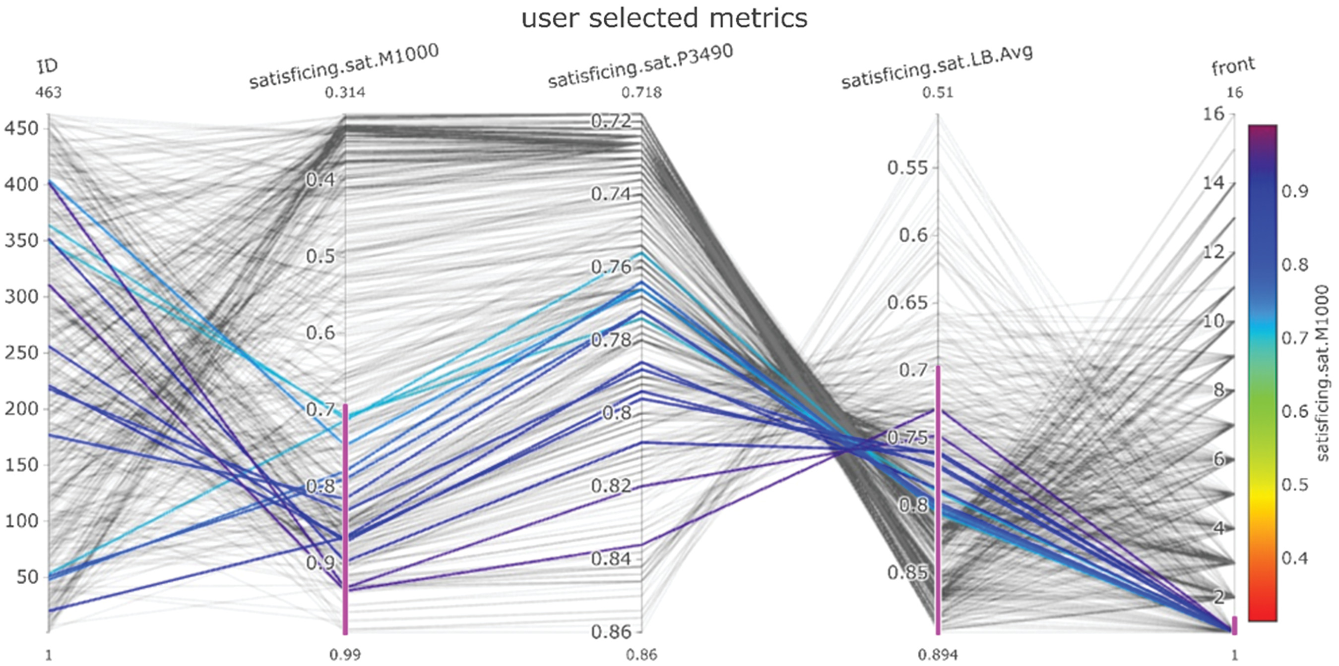
Next, we use on-the-fly nondominated sorting to select policies that perform well with respect to our custom satisficing metrics. We describe the process below, and the result is shown in Fig. 5. First, we navigate to the Select your own page and click the select metrics button. We select our satisficing metrics by choosing satisficing under the metric 1 type button, then selecting sat.M1000 with the metric 1: button. We repeat this process to select sat.P3490 and sat.LB.Avg under the autocreated metric 2: and metric 3: buttons. After clicking apply selected metrics, our metrics are added to the PC plot. The satisficing metrics are labelled with the prefix satisficing.sat (e.g., satisficing.sat.M1000). A value of one indicates the performance threshold is satisfied in all SOW, and zero indicates the requirement is never satisfied (see Fig. 3). Next, we select the Calculate fronts button, which adds an axis to the far right labeled front. A policy belongs to the first front, if it is nondominated with respect to the three satisficing metrics. To select the nondominated policies, we use a brush filter by clicking and dragging over front = 1 (see the heavy pink line at 1 on the front axis in Fig. 5). Note that sat.P3490 is always greater than 0.7, but sat.M1000 and sat.LB.Avg are as low as 0.31 and 0.51, respectively. We choose to balance the three satisficing metrics, so we use brushing to select policies with at least 0.7 for both sat.M1000 and sat.LB.Avg. We used brush filters in this example, but the stakeholder can manually type thresholds using the manual filters button in the left sidebar (Fig. 4). After selecting the save brush filters button, 14 policies remain.
Phase 2: Refining Robustness Preferences
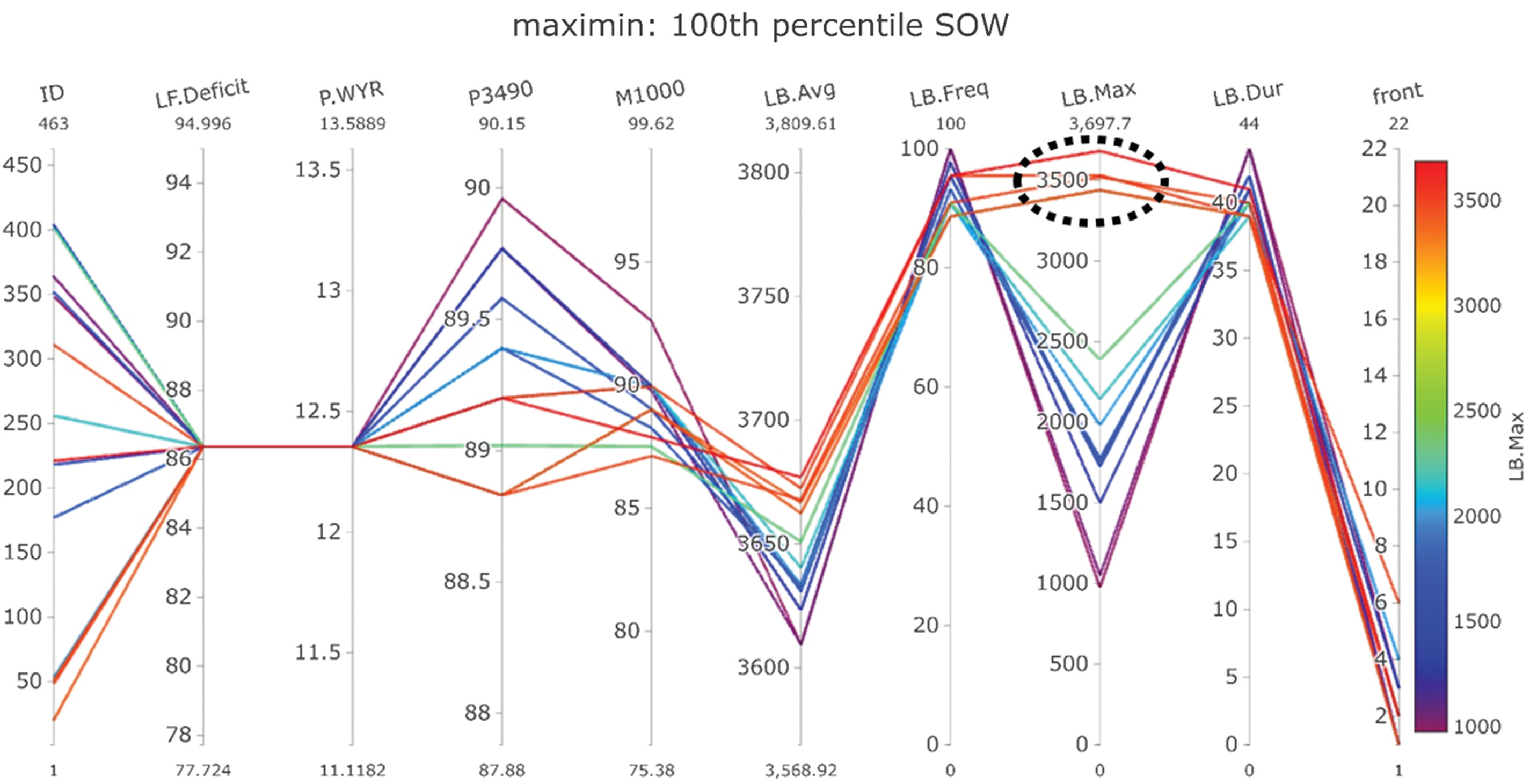
Next, we explore trade-offs of the remaining policies with additional robustness metrics using global linking. While on the Select your own page, we select the save filters globally button, which indicates only the remaining policies will be shown on other pages and tabs. For example, we navigate to the Robustness metrics page and maximin tab, which shows the worst performance across all SOW for the specified objective (see description in Fig. 3). The resulting PC plot is also shown in Fig. 6. This metric reflects a high level of risk aversion (McPhail et al. 2018, 2021), which is a common preference of water providers (Smith et al. 2017). Only the 14 remaining policies are shown, but, importantly, the range of each axis shows the possible values across all 463 policies. Five policies result in severe annual shortages (the LB.Max axis), annotated with the black-dotted oval in Fig. 6. There remain other policies that reduce maximum annual shortages by 1,000 KAF or more (seen by the gap between the policies within the oval and those below 2,500 KAF). To remove the severe-shortage policies, we use a brush filter to highlight the policies below 2,500 KAF on the LB.Max axis and select save brush filters. During this step, we added an additional robustness metric to our initial selection because of the trade-offs we discovered, leaving nine policies remaining.
Choosing Policies with Interactive Data Tables
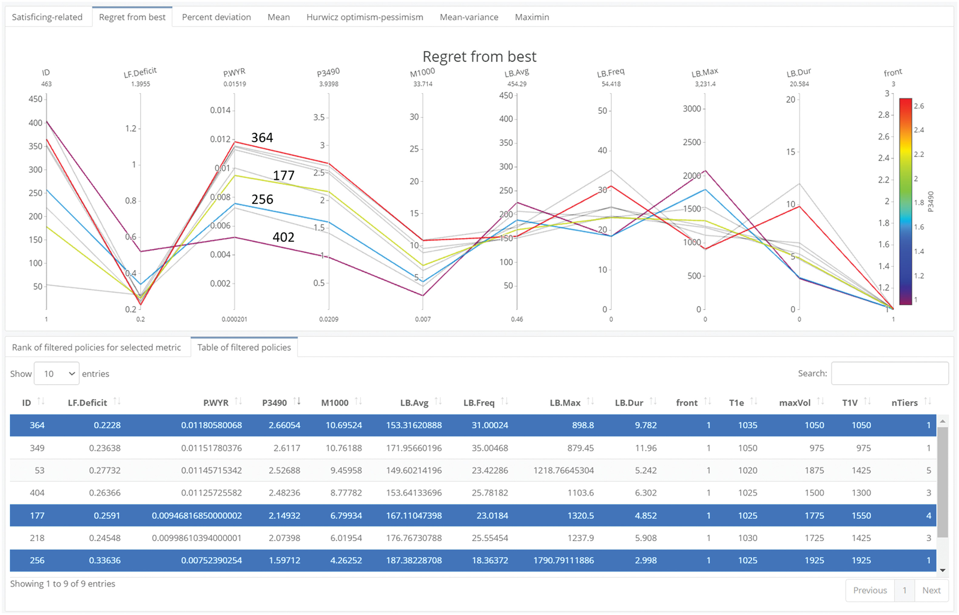
Next, we select a small number of interesting policies, which could become the focus of deliberation or interrogated further in a vulnerability analysis. One way to accomplish this, besides with brush or manual filters, is through an interactive data table. To do so, select save filters globally, navigate to the Regret from best tab, and select the Table of filtered policies tab. The result is shown in Fig. 7. This metric describes the deviation of a policy’s performance from the best performing policy, averaged across the SOW (Fig. 3). Because public agencies can be criticized when, in hindsight, the decision made could have yielded better results, this metric may be of interest to water resources agencies (McPhail et al. 2021). Indicated by crossing lines, Fig. 7 shows that reservoir storage (M1000 and P3490) trades off with average shortage (LB.Avg), and that average shortage trades off with frequency of shortage (LB.Freq). As shown in Fig. 7, in the table, we use the interactive data table to select (by clicking on) one policy that prioritizes reservoir storage (ID 402), one with low average shortage (ID 364), and two that balance the trade-offs (IDs 256 and 177). The resulting shortage policies (Fig. 8) can be viewed by selecting the keep button under table selections: in the left sidebar, then navigating back to Rank of filtered policies for selected metric tab. In Fig. 8, the policies are ranked ordered according to the P3490 objective and regret from best metric, which can be changed with the Metric for ranking button in the left sidebar.

Decision Provenance for Reproducibility and Communication
Because our framework allows for unique, dynamic, and multistep analyses, it is important that the results are reproducible. So, the app uses an activity log to track the objectives/robustness metrics that filters are applied to and the corresponding filter criteria. The activity log is downloaded as a spreadsheet using the Download button at the lower left of Fig. 2. A screenshot of the activity log for this demonstration is in the Appendix.
It is also important that the results are easily communicated between stakeholders. As such, all PC plots and DV plots are downloadable, and several download parameters can be adjusted to fit the needs of reports and presentations. Plot settings are accessed with the blue plot options button (to the right of the Download button in Fig. 2). The PC plots are highly adjustable, with settings for color palette, title size, label size and angles, image size, and file type. For example, Figs. 5, 6, and 8 were downloaded directly from the app.
Discussion and Conclusion
This research demonstrates a robustness tradeoff analysis of Lake Mead shortage policies using an interactive web app. In our analysis, we show how a posteriori robustness exploration can reveal significant trade-offs that refine stakeholders’ robustness definitions and rapidly remove nonrobust policies. We tested if existing performance thresholds and the satisficing metric were sufficient to identify robust shortage policies. Using nondominated robustness sorting and interactive PC plots, we identified policies that are robust with respect to the three satisficing metrics. Because performance thresholds were already established in previous research (Alexander 2018), existing robustness frameworks suggest that it would be appropriate to choose policies based on the satisficing metric alone (McPhail et al. 2018, 2021). However, using our framework, we discovered that several remaining policies resulted in very severe LB shortages (the maximin metric), roughly 1 MAF larger than the other remaining policies. Had we chosen policies based on our initial priorities (the three satisficing metrics), this knowledge would have gone undiscovered. Instead, our a posteriori framework challenged and refined our initial preferences, and the policies resulting in severe LB shortages were removed. Finally, we demonstrated how other tools in our framework, such as data tables, marking, and activity logs, help stakeholders choose a small number of policies and communicate their decision to others.
We see several opportunities for future research. First, we hope that future studies apply our framework to new decision problems. Although the app as presented in this article uses CRB data, it can be modified for other studies by changing the underlying database of policies, performance objectives, and robustness metrics. We refer the interested reader to our GitHub repository (Bonham 2023), which includes the source code and instructions to download and run the app locally. Building on our robustness framework, future research could investigate the effectiveness of interactive web tools for other robust decision making techniques, such as vulnerability analysis (Bryant and Lempert 2010; Hadjimichael et al. 2020b), adaptation pathways (Haasnoot et al. 2013), and negotiation (Bonham et al. 2022; Gold et al. 2019). Our framework uses an activity log to make the robustness analysis reproducible and communicable, an example of provenance. Future research could build on this effort with recent advances in provenance methods that record what insights were learned during an analysis, the rationale behind decisions, and integrate the provenance information into interactive visualizations (Chakhchoukh et al. 2022; Ragan et al. 2016). Such methods could improve the efficacy of a posteriori methods for decision support. Given the rise in interactive web apps for education (Peñuela et al. 2021) and decision support (Raseman et al. 2019), future research could use workshops, surveys, and retrospective studies to test their efficacy and guide future research questions (Pianosi et al. 2020; Smith et al. 2017).
Through demonstrating our a posteriori framework, our research opens up further opportunities for collaborative MORDM analyses. For example, we used the CRB robustness app in a participatory workshop where Reclamation explored robustness metrics, applied the interactive filtering tools, and tested the various mechanisms for customizing robustness metrics and PC plots. Building on our collaboration, Reclamation is adopting and expanding the CRB robustness app for use in post-2026 planning (Reclamation 2023b; Smith et al. 2022). Reclamation will use the expanded app to communicate policy performance, robustness, and vulnerability to solicit preferences from a diverse group of stakeholders including water utilities, state agencies, irrigation districts, environmental agencies and Tribal leadership. In parallel with the app development, Reclamation is holding training sessions to ensure stakeholders can meaningfully engage with the tools (Reclamation 2023b). We believe our app and Reclamation’s ongoing development are a significant milestone in the adoption of robust decision-making techniques in collaborative, international water resources management. We encourage future studies to develop decision support frameworks and tools in collaboration with end users to improve their efficacy, increase likelihood of organizational uptake, and expedite their real-world application (Stanton and Roelich 2021).
Appendix. Activity Log of Example Robustness Analysis
The activity log for the example analysis above is shown in Fig. 9. The activity log tracks which pages, robustness metrics/objectives, and filters were used to arrive at the chosen policies.

Data Availability Statement
Some or all data, models, or code generated or used during the study are available at the corresponding author’s GitHub repository: https://github.com/nabocrb/CRB-robustness-app---JWRPM (Bonham 2023).
Acknowledgments
We thank Reclamation for providing the Lake Mead policies and input on the app’s design. We also thank anonymous reviewers who helped improve the clarity of this article. This research is based on work supported by Reclamation’s Upper and Lower Colorado regions Science Foundation Graduate Research Fellowship under Grant No. DGE 2040434.
References
Alexander, E. 2018. “Searching for a robust operation of Lake Mead.” Accessed April 1, 2022. https://www.colorado.edu/cadswes/sites/default/files/attached-files/searching_for_a_robust_operation_of_lake_mead_2018.pdf.
Ben-Haim, Y. 2004. “Uncertainty, probability and information gaps.” Reliab. Eng. Syst. Saf. 85 (1): 249–266. https://doi.org/10.1016/j.ress.2004.03.015.
Bonham, N. 2023. “CRB robustness tradeoffs.” Accessed December 26, 2023. https://nabocrb.shinyapps.io/CRB-Robustness-App-JWRPM/.
Bonham, N., J. Kasprzyk, and E. Zagona. 2022. “post-MORDM: Mapping policies to synthesize optimization and robustness results for decision-maker compromise.” Environ. Modell. Software 157 (Nov): 105491. https://doi.org/10.1016/j.envsoft.2022.105491.
Brill, E. D., J. M. Flach, L. D. Hopkins, and S. Ranjithan. 1990. “MGA: A decision support system for complex, incompletely defined problems.” IEEE Trans. Syst. Man Cybern. 20 (4): 745–757. https://doi.org/10.1109/21.105076.
Brown, C., Y. Ghile, M. Laverty, and K. Li. 2012. “Decision scaling: Linking bottom-up vulnerability analysis with climate projections in the water sector.” Water Resour. Res. 48 (9). https://doi.org/10.1029/2011WR011212.
Bryant, B. P., and R. J. Lempert. 2010. “Thinking inside the box: A participatory, computer-assisted approach to scenario discovery.” Technol. Forecasting Social Change 77 (1): 34–49. https://doi.org/10.1016/j.techfore.2009.08.002.
Buschatzke, T., E. James, P. Nelson, J. Entsminger, J. D’Antonio, P. Tyrrell, and E. Millis. 2019. “UDrought contingency plans–Basin states transmittal letter to congress.” Accessed March 19, 2019. https://www.usbr.gov/dcp/docs/DroughtContigencyPlansBasinStates-TransmittalLetter-508-DOI.pdf.
Chakhchoukh, M. R., N. Boukhelifa, and A. Bezerianos. 2022. “Understanding how in-visualization provenance can support trade-off analysis.” IEEE Trans. Visual Comput. Graphics 29 (9): 3758–3774. https://doi.org/10.1109/TVCG.2022.3171074.
Chang, W., et al. 2022. Shiny: Web application framework for R. Birmingham, UK: Packt.
Gangopadhyay, S., C. A. Woodhouse, G. J. McCabe, C. C. Routson, and D. M. Meko. 2022. “Tree rings reveal unmatched 2nd century drought in the Colorado River basin.” Geophys. Res. Lett. 49 (11): e2022GL098781. https://doi.org/10.1029/2022GL098781.
Gold, D. F., P. M. Reed, B. C. Trindade, and G. W. Characklis. 2019. “Identifying actionable compromises: Navigating multi-city robustness conflicts to discover cooperative safe operating spaces for regional water supply portfolios.” Water Resour. Res. 55 (11): 9024–9050. https://doi.org/10.1029/2019WR025462.
Haasnoot, M., J. H. Kwakkel, W. E. Walker, and J. ter Maat. 2013. “Dynamic adaptive policy pathways: A method for crafting robust decisions for a deeply uncertain world.” Global Environ. Change 23 (2): 485–498. https://doi.org/10.1016/j.gloenvcha.2012.12.006.
Hadjimichael, A., D. Gold, D. Hadka, and P. Reed. 2020a. “Rhodium: Python library for many-objective robust decision making and exploratory modeling.” J. Open Res. Software 8 (1): 12. https://doi.org/10.5334/jors.293.
Hadjimichael, A., J. Quinn, E. Wilson, P. Reed, L. Basdekas, D. Yates, and M. Garrison. 2020b. “Defining robustness, vulnerabilities, and consequential scenarios for diverse stakeholder interests in institutionally complex river basins.” Earth’s Future 8 (7): e2020EF001503. https://doi.org/10.1029/2020EF001503.
Hadka, D. 2015. “Introducing OpenMORDM.” Accessed October 28, 2019. https://waterprogramming.wordpress.com/2015/10/01/introducing-openmordm/.
Hadka, D., and P. Reed. 2013. “Borg: An auto-adaptive many-objective evolutionary computing framework.” Evol. Comput. 21 (2): 231–259. https://doi.org/10.1162/EVCO_a_00075.
Herman, J. D., P. M. Reed, H. B. Zeff, and G. W. Characklis. 2015. “How should robustness be defined for water systems planning under change?” J. Water Resour. Plann. Manage. 141 (10): 04015012. https://doi.org/10.1061/(ASCE)WR.1943-5452.0000509.
Herman, J. D., H. B. Zeff, P. M. Reed, and G. W. Characklis. 2014. “Beyond optimality: Multistakeholder robustness trade-offs for regional water portfolio planning under deep uncertainty.” Water Resour. Res. 50 (10): 7692–7713. https://doi.org/10.1002/2014WR015338.
Inselberg, A. 2009. Parallel coordinates. New York: Springer.
International Boundary and Water Commission. 2012. “Minute 319: Interim international cooperative measures in the Colorado River Basin through 2017 and extension of minute 318 cooperative measures to address the continued effects of the April 2010 earthquake in the Mexicali Valley, Baja California.” Accessed November 7, 2023. https://www.ibwc.gov/Files/Minutes/Minute_319.pdf.
International Boundary and Water Commission. 2017. “Minute 323: Extension of cooperative measures and adoption of a binational water scarcity contingency plan in the Colorado River Basin.” Accessed November 7, 2023. https://www.usbr.gov/lc/region/g4000/4200Rpts/DecreeRpt/2018/43.pdf.
Jafino, B. A., and J. H. Kwakkel. 2021. “A novel concurrent approach for multiclass scenario discovery using multivariate regression trees: Exploring spatial inequality patterns in the Vietnam Mekong Delta under uncertainty.” Environ. Modell. Software 145 (Nov): 105177. https://doi.org/10.1016/j.envsoft.2021.105177.
James, T., A. Evans, E. Madly, and C. Kelly. 2014. “The economic importance of the Colorado River to the basin region.” Accessed November 7, 2023. https://businessforwater.org/wp-content/uploads/2016/12/PTF-Final-121814.pdf.
Kasprzyk, J. R., S. Nataraj, P. M. Reed, and R. J. Lempert. 2013. “Many objective robust decision making for complex environmental systems undergoing change.” Environ. Modell. Software 42 (Apr): 55–71. https://doi.org/10.1016/j.envsoft.2012.12.007.
Kasprzyk, J. R., P. M. Reed, G. W. Characklis, and B. R. Kirsch. 2012. “Many-objective de Novo water supply portfolio planning under deep uncertainty.” Environ. Modell. Software 34 (May): 87–104. https://doi.org/10.1016/j.envsoft.2011.04.003.
Knight, F. 1921. Risk, uncertainty, and profit. Boston: Houghton Mifflin.
Kollat, J. B., and P. Reed. 2007. “A framework for visually interactive decision-making and design using evolutionary multi-objective optimization (VIDEO).” Environ. Modell. Software 22 (12): 1691–1704. https://doi.org/10.1016/j.envsoft.2007.02.001.
Kwakkel, J. H. 2017. “The exploratory modeling workbench: An open source toolkit for exploratory modeling, scenario discovery, and (multiobjective) robust decision making.” Environ. Modell. Software 96 (Oct): 239–250. https://doi.org/10.1016/j.envsoft.2017.06.054.
Kwakkel, J. H., and M. Haasnoot. 2019. “Supporting DMDU: A taxonomy of approaches and tools.” In Decision making under deep uncertainty: From theory to practice, edited by V. A. W. J. Marchau, W. E. Walker, P. J. T. M. Bloemen, and S. W. Popper, 355–374. Cham, Switzerland: Springer.
Lempert, R. J., D. G. Groves, S. W. Popper, and S. C. Bankes. 2006. “A general, analytic method for generating robust strategies and narrative scenarios.” Manage. Sci. 52 (4): 514–528. https://doi.org/10.1287/mnsc.1050.0472.
Lempert, R. J., S. W. Popper, and S. C. Bankes. 2003. “Shaping the next one hundred years: New methods for quantitative, long-term policy analysis.” RAND Corporation. Accessed January 10, 2022. https://www.rand.org/pubs/monograph_reports/MR1626.html.
Lukas, J., and E. Payton. 2020. “Colorado River basin climate and hydrology: State of the science.” Accessed November 23, 2021. https://scholar.colorado.edu/concern/reports/8w32r663z.
Maier, H. R., S. Razavi, Z. Kapelan, L. S. Matott, J. Kasprzyk, and B. A. Tolson. 2019. “Introductory overview: Optimization using evolutionary algorithms and other metaheuristics.” Environ. Modell. Software 114 (Apr): 195–213. https://doi.org/10.1016/j.envsoft.2018.11.018.
McPhail, C., H. R. Maier, J. H. Kwakkel, M. Giuliani, A. Castelletti, and S. Westra. 2018. “Robustness metrics: How are they calculated, when should they be used and why do they give different results?” Earth’s Future 6 (2): 169–191. https://doi.org/10.1002/2017EF000649.
McPhail, C., H. R. Maier, S. Westra, J. H. Kwakkel, and L. Linden. 2020. “Impact of scenario selection on robustness.” Water Resour. Res. 56 (9): e2019WR026515. https://doi.org/10.1029/2019WR026515.
McPhail, C., H. R. Maier, S. Westra, L. van der Linden, and J. H. Kwakkel. 2021. “Guidance framework and software for understanding and achieving system robustness.” Environ. Modell. Software 142 (Aug): 105059. https://doi.org/10.1016/j.envsoft.2021.105059.
Minasny, B., and A. B. McBratney. 2006. “A conditioned Latin hypercube method for sampling in the presence of ancillary information.” Comput. Geosci. 32 (9): 1378–1388. https://doi.org/10.1016/j.cageo.2005.12.009.
Peñuela, A., C. Hutton, and F. Pianosi. 2021. “An open-source package with interactive Jupyter Notebooks to enhance the accessibility of reservoir operations simulation and optimisation.” Environ. Modell. Software 145 (Nov): 105188. https://doi.org/10.1016/j.envsoft.2021.105188.
Pianosi, F., F. Sarrazin, and T. Wagener. 2020. “How successfully is open-source research software adopted? Results and implications of surveying the users of a sensitivity analysis toolbox.” Environ. Modell. Software 124 (Feb): 104579. https://doi.org/10.1016/j.envsoft.2019.104579.
Quinn, J. D., A. Hadjimichael, P. M. Reed, and S. Steinschneider. 2020. “Can exploratory modeling of water scarcity vulnerabilities and robustness be scenario neutral?” Earth’s Future 8 (11): e2020EF001650. https://doi.org/10.1029/2020EF001650.
Ragan, E., E. Alex, J. Sanyal, and J. Chen. 2016. “Characterizing provenance in visualization and data analysis: An organizational framework of provenance types and purposes.” IEEE Trans. Visual Comput. Graphics 22 (1): 31–40. https://doi.org/10.1109/TVCG.2015.2467551.
Raseman, W. J., J. Jacobson, and J. R. Kasprzyk. 2019. “Parasol: An open source, interactive parallel coordinates library for multi-objective decision making.” Environ. Modell. Software 116 (Jun): 153–163. https://doi.org/10.1016/j.envsoft.2019.03.005.
R Core Team. 2022. R: A language and environment for statistical computing. Vienna, Australia: R Foundation for Statistical Computing.
Reclamation. 2007. “Colorado River interim guidelines for lower basin shortage and coordinated operations for Lakes Powell and Mead–Final environmental impact statement.” Accessed February 22, 2020. https://www.usbr.gov/lc/region/programs/strategies/FEIS/ExecSumm.pdf.
Reclamation. 2011. “Lake Mead area and capacity tables.” Accessed October 18, 2022. https://www.usbr.gov/lc/region/g4000/LM_AreaCapacityTables2009.pdf.
Reclamation. 2012. “Colorado River basin water supply and demand study.” Accessed August 30, 2019. https://www.usbr.gov/lc/region/programs/crbstudy/finalreport/Study%20Report/CRBS_Study_Report_FINAL.pdf.
Reclamation. 2020. “5-Year probabilistic projections.” Accessed January 11, 2022. https://www.usbr.gov/lc/region/g4000/riverops/crss-5year-projections.html.
Reclamation. 2023a. “Lower Colorado water supply report.” Accessed October 30, 2023. https://www.usbr.gov/lc/region/g4000/weekly.pdf.
Reclamation. 2023b. “Post-2026 Colorado River reservoir operational strategies for Lake Powell and Lake Mead.” Accessed March 6, 2023. https://www.usbr.gov/ColoradoRiverBasin/Post2026Ops.html.
Reis, J., and J. Shortridge. 2020. “Impact of uncertainty parameter distribution on robust decision making outcomes for climate change adaptation under deep uncertainty.” Risk Anal. 40 (3): 494–511. https://doi.org/10.1111/risa.13405.
Root, J. C., and D. Jones. 2022. “Elevation-area-capacity relationships of Lake Powell in 2018 and estimated loss of storage capacity since 1963. Elev.-Area-Capacity Relatsh. Lake Powell 2018 Estim. Loss storage capacity 1963, Scientific investigations Report, 21. USGS numbered series.” Accessed February 21, 2023. http://pubs.er.usgs.gov/publication/sir20225017.
Roy, B. 1990. “Decision-aid and decision-making.” Eur. J. Oper. Res. 45 (2–3): 324–331. https://doi.org/10.1016/0377-2217(90)90196-I.
Salehabadi, H., D. G. Tarboton, B. Udall, K. G. Wheeler, and J. C. Schmidt. 2022. “An assessment of potential severe droughts in the Colorado River basin.” JAWRA J. Am. Water Resour. Assoc. 58 (6): 1053–1075. https://doi.org/10.1111/1752-1688.13061.
Sievert, C. 2020. Interactive web-based data visualization with R, plotly, and shiny. Boca Raton, FL: CRC Press.
Sievert, C., et al. 2023. “flexdashboard: R markdown format for flexible dashboards.” Accesssed August 11, 2023. https://CRAN.R-project.org/package=flexdashboard.
Smith, R., J. Kasprzyk, and L. Basdekas. 2018. “Experimenting with water supply planning objectives using the eldorado utility planning model multireservoir testbed.” J. Water Resour. Plann. Manage. 144 (8): 04018046. https://doi.org/10.1061/(ASCE)WR.1943-5452.0000962.
Smith, R., J. Kasprzyk, and L. Dilling. 2017. “Participatory framework for assessment and improvement of tools (ParFAIT): Increasing the impact and relevance of water management decision support research.” Environ. Modell. Software 95 (Sep): 432–446. https://doi.org/10.1016/j.envsoft.2017.05.004.
Smith, R., J. Kasprzyk, and L. Dilling. 2019. “Testing the potential of multiobjective evolutionary algorithms (MOEAs) with Colorado water managers.” Environ. Modell. Software 117 (Jul): 149–163. https://doi.org/10.1016/j.envsoft.2019.03.011.
Smith, R., E. Zagona, J. Kasprzyk, N. Bonham, E. Alexander, A. Butler, J. Prairie, and C. Jerla. 2022. “Decision science can help address the challenges of long-term planning in the Colorado River basin.” JAWRA J. Am. Water Resour. Assoc. 58 (5): 735–745. https://doi.org/10.1111/1752-1688.12985.
Stanton, M. C. B., and K. Roelich. 2021. “Decision making under deep uncertainties: A review of the applicability of methods in practice.” Technol. Forecasting Social Change 171 (Oct): 120939. https://doi.org/10.1016/j.techfore.2021.120939.
Upper Colorado River Commission. 2016. “2016 Upper Colorado River basin depletion demand schedules.” Accessed November 7, 2023. http://www.ucrcommission.com/RepDoc/DepSchedules/CurFutDemandSchedule.pdf.
Wickham, H. 2016. ggplot2: Elegant graphics for data analysis. 2nd ed. Berlin: Springer. https://doi.org/10.1007/978-3-319-24277-4.
Wickham, H., R. François, L. Henry, K. Müller, and D. Vaughan. 2023. “dplyr: A grammar of data manipulation.” Accesssed November 17, 2023. https://CRAN.R-project.org/package=dplyr.
Woodruff, M. J., P. M. Reed, and T. W. Simpson. 2013. “Many objective visual analytics: Rethinking the design of complex engineered systems.” Struct. Multidiscip. Optim. 48 (1): 201–219. https://doi.org/10.1007/s00158-013-0891-z.
Zagona, E. A., T. J. Fulp, R. Shane, T. Magee, and H. M. Goranflo. 2001. “Riverware: A generalized tool for complex reservoir system modeling.” JAWRA J. Am. Water Resour. Assoc. 37 (4): 913–929. https://doi.org/10.1111/j.1752-1688.2001.tb05522.x.
Zeleny, M. 1989. “Cognitive equilibrium: A new paradigm of decision making?” Hum. Syst. Manage. 8 (3): 185–188. https://doi.org/10.3233/HSM-1989-8301.
Information & Authors
Information
Published In

Journal of Water Resources Planning and Management
Volume 150 • Issue 3 • March 2024
Copyright
This work is made available under the terms of the Creative Commons Attribution 4.0 International license, https://creativecommons.org/licenses/by/4.0/.
History
Received: Mar 24, 2023
Accepted: Aug 28, 2023
Published online: Dec 30, 2023
Published in print: Mar 1, 2024
Discussion open until: May 30, 2024
ASCE Technical Topics:
- Basins
- Bodies of water (by type)
- Case studies
- Computer networks
- Computer vision and image processing
- Computing in civil engineering
- Engineering fundamentals
- Interactive systems
- Internet
- Lakes
- Measurement (by type)
- Methodology (by type)
- Metric systems
- Research methods (by type)
- River engineering
- Rivers and streams
- Systems engineering
- Systems management
- Water and water resources
- Water management
Authors
Metrics & Citations
Metrics
Citations
Download citation
If you have the appropriate software installed, you can download article citation data to the citation manager of your choice. Simply select your manager software from the list below and click Download.