Urban Flood Inundation Probability Assessment Based on an Improved Bayesian Model
Abstract
Urban flood inundation is spatially uncertain. To quantify this uncertainty, it is necessary to explore the spatial probability of urban flood inundation in different return periods. In this study, an urban flood spatial inundation probability assessment method based on an improved Bayesian model is proposed, which comprises three parts: data reconstruction based on undersampling; optimal Bayesian sample planning; and spatial inundation probability assessment. A case study of the central urban area of Jingdezhen City, China, is presented in this paper. The results indicate that (1) the inundation probabilities generated based on various return periods (20-, 50-, and 100-year return periods) are accurately determined and can provide more detailed inundation information. (2) The adoption of the random undersampling data reconstruction method solves the problem of an imbalanced number of inundations/noninundations during Bayesian modeling and substantially enhances the prediction accuracy compared with the traditional Bayesian modeling approach. (3) A sensitivity analysis reveals that inundation probability is sensitive to the drainage network and elevation rather than soil water retention and distance to river. With an increase in the return period, the inundation probability gradually increases. As the proposed method can quantify flood inundation uncertainty, it is valuable in supporting specific flood risk assessments.
Introduction
Ongoing urbanization has caused urban flood disasters to become increasingly serious (Jamali et al. 2018). Urban flood inundation causes water accumulation on roads and residences, which can severely interrupt traffic and damages private property. Serious urban flood inundation accidents have occurred worldwide. For example, on September 1, 2021, Hurricane Ida barreled into New York City, causing severe flooding and 13 deaths and disrupting transit across parts of New York. From July 17 to 21, 2021, catastrophic flooding affected Zhengzhou, Henan, in China, causing severe flood damage to property, motor, public transportation, and infrastructure; 73 people were killed. Urban flood risk assessment can provide an effective approach to prevent and mitigate the adverse effects of disasters (UNISDR 2009). A flood map shows the inundation area, inundation range, and inundation depth and can be employed for risk identification (Sun et al. 2020). However, urban flood inundation is spatially uncertain. Some areas may be inundated more frequently, whereas other areas may be inundated less frequently. It is necessary to not only explore whether certain areas will be inundated in different return periods but also to better understand the inundation probability.
In previous studies, flood maps have generally been obtained from hydrological or hydrodynamic model simulations, which involve physically based hydrologic processes (Bajabaa et al. 2013; Chen et al. 2012). These methods, however, are overly dependent on large amounts of data, such as pipeline data, fine-resolution topography data, and flood control facilities, some of which are difficult to obtain. Although hydrological or hydrodynamic models can be developed using a probabilistic approach, which derives an uncertain flood extent map due to uncertainty in model parameters (Merwade et al. 2008; Di Baldassarre et al. 2010), establishing these models is difficult and inefficient, especially in a rapid urbanization context. In the era of big data and machine learning, simplified models have calculated inundation probability by focusing on the relationships between relevant factors and inundation areas. Wang et al. (2015b) used random forest to evaluate regional flood hazard risk. Tang et al. (2018) used a weighted naïve Bayes classifier to assess the spatial urban waterlogging risk. Li et al. (2010) constructed a Bayesian network to integrate multiple factors for the assessment of catastrophic risk. The Bayesian method can include the key urban environmental factors in probabilistic modeling and also can be utilized to explore the quantitative relationship between these factors and numerous historical events. The method has been used to estimate the likelihood of various disasters, including earthquakes (Han et al. 2019; Cockburn and Tesfamariam 2012), debris flows (Liang et al. 2012), and forest fires (Sevinc et al. 2020). In flood risk assessment, in particular, a spatial inundation assessment model based on a combination of Bayesian and geographic information system (GIS) methods has been proposed and applied in the Bowen Basin, Australia (Liu et al. 2016, 2017), and Guangzhou, China (Tang et al. 2018). However, this method may cause over- or underestimation of the flood inundation probability, as it is based on the superimposition of maximum inundation areas throughout a given historical period without considering the flood frequency factor. To rectify this shortcoming, different return periods of floods should be considered to calculate flood inundation probability.
Moreover, the Bayesian method assumes that the number of samples in each category is approximately balanced. However, flood inundation areas are generally concentrated only within a certain part of an urban area; therefore, the size of inundation observation samples is much smaller than that of noninundation areas. Such an imbalance can cause the model to focus too much on major sample data, whereas key minor data could be omitted during the training process (Krawczyk 2016). Therefore, the problem of an imbalanced sample size between inundation data and noninundation data should be solved in the very first step. The resampling method is widely adopted to reconstruct data to address this problem (Mohammed et al. 2020), including over- and undersampling techniques. The oversampling method expands the number of minority class examples to balance the class distribution, while the undersampling method eliminates the majority class examples randomly. It has been found that the undersampling technique, when combined with the naïve Bayes method, can decrease the training time while increasing the classification performance (Aridas et al. 2019).
In this study, an improved Bayesian method through data reconstruction is presented to assess the spatial inundation probability of urban floods under different return periods. Therefore, the primary objectives of the present study are as follows: (1) to construct a balanced data set using undersampling techniques for the Bayesian model through data reconstruction conception; (2) to obtain flood inundation probability maps for different return periods and to analyze the flood inundation probability; and (3) to analyze the sensitivity of key urban factors to the flood inundation probability.
Methods
Overall Framework of the Urban Flood Inundation Probability Assessment Method
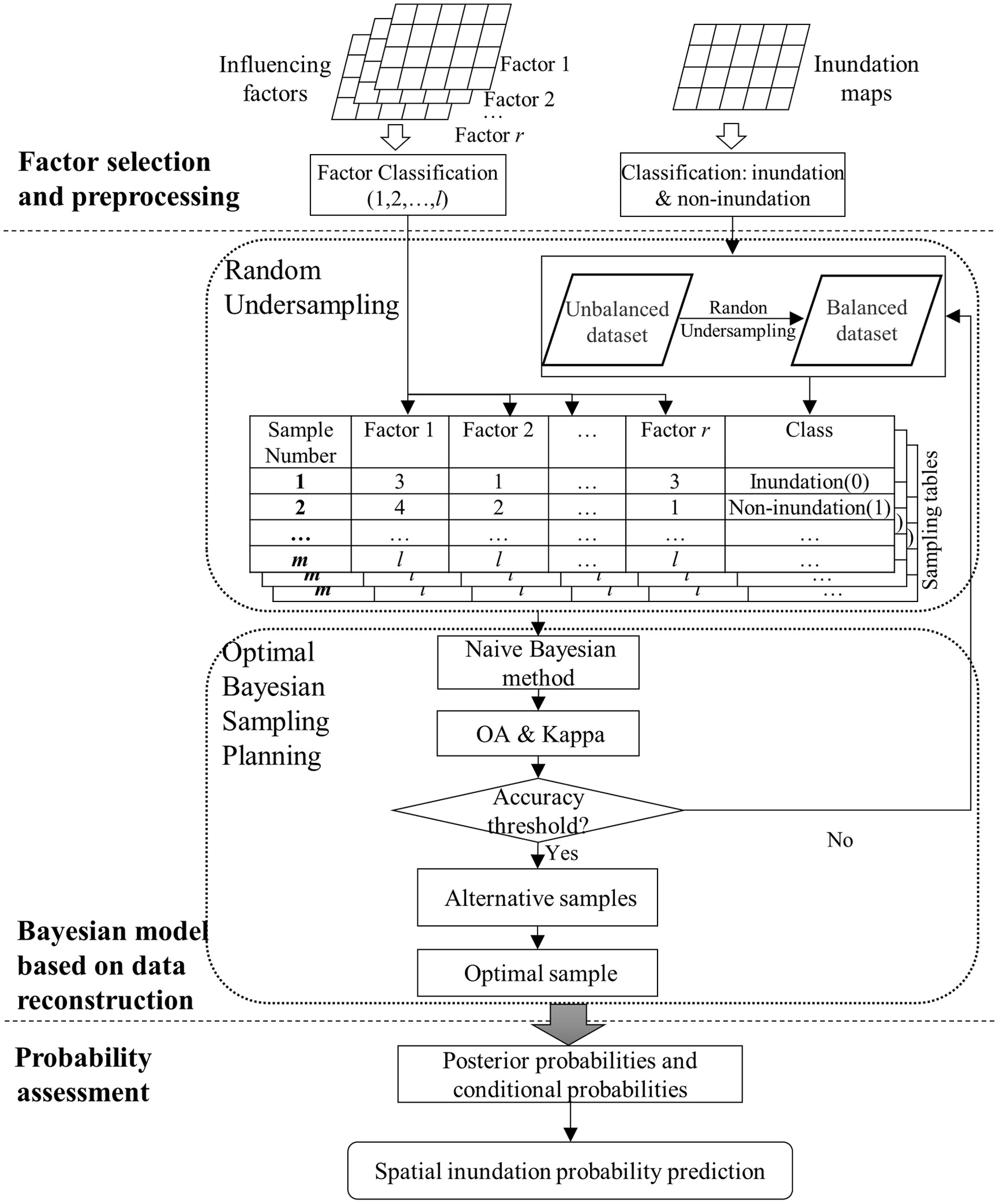
The proposed framework, which is shown in Fig. 1, includes three modules: data reconstruction based on undersampling; optimal Bayesian sample planning; and spatial inundation probability assessment. Before data reconstruction, the influencing factors should be selected by analyzing the flood inundation formation process according to previous studies. Once selected, these grid-based data sets are then standardized and classified into several classes, which are applied as inputs of the naïve Bayes model. The inundation maps under different return periods are also classified into inundation and noninundation. A detailed process is presented in the section “Data Collection and Processing.” Due to the imbalance between inundation data and noninundation data, the random undersampling technique is adopted to generate the optimal Bayesian sample. These two steps are described in the section “Module of the Bayesian Model Based on Data Reconstruction.” Based on the optimal Bayesian sample, the posterior probability in each grid can then be determined based on the conditional probability. The model is described in the section “Probability Assessment Based on the Naïve Bayesian Model.” Further, to identify the most sensitive urban factors resulting in inundation, the contribution of each selected factor to the overall probability is estimated based on the derivative function, as introduced in the section “Sensitivity Analysis.”
Module of the Bayesian Model Based on Data Reconstruction
Bayesian model establishment based on data reconstruction includes two steps: data reconstruction based on undersampling and optimal Bayesian sample planning. In the first step, noninundation grids are equally divided into several groups according to the geographical location, and random undersampling is then adopted to select noninundation grids from each group. A balanced data set is generated. In the second step, an optimal sample can be generated based on the naïve Bayesian training process.
Data Reconstruction Based on Undersampling
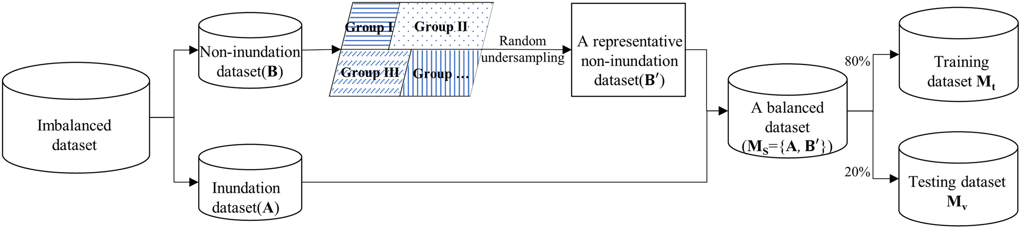
First, all grids from the inundation map under a certain return period are divided into two data sets: the noninundation data set (Set B) and inundation data set (Set A). Random undersampling is adopted to select samples from Set B to establish a representative Set . In order to overcome the disadvantage of missing important samples in traditional random undersampling, the -means clustering technique is implemented to divide the noninundation data set into several equal groups based on the geographic projected coordinates. Therefore, the noninundation grids from different locations can be collected by randomly sampling each group. Then, the number of Set is the same as that of Set A. Last, a balanced data set is reconstructed by combining inundation grids (Set A) and selected noninundation grids (Set ), which is . It is divided into two sets: a training set with 80% of the grids and a testing set with 20%. The process is shown in Fig. 2.
Optimal Bayesian Sample Plan
As the random sampling method is employed to reconstruct the observation data set, a new data set can be generated with a random sampling process every time. There are a number of different balanced training sets, , . To ensure the accuracy of the probability assessment model, it is necessary to screen the training set with the optimal accuracy through multiple sampling and accuracy evaluation iterations. Therefore, the naïve Bayes method is adopted to train these samples, and accuracy evaluation is carried out until the optimal sample data table with the highest accuracy is determined.
Naïve Bayes is a statistical classification technique that determines the class used for classification based on the hypothesis that attributes are independent of each other. The naïve Bayes model collects an example occurrence of an event and estimates the prior probability for each class. The advantage of the naïve Bayes model is that it is possible to estimate the parameters needed for classification with a small amount of learning data (Lee et al. 2020).
The naïve Bayes correlation equation is calculated following Eq. (1)where = the prior probability of the class node; = the conditional probability; and = the posterior probability. In this study, inundation or noninundation conditions are considered nodes , and the selected urban factors are considered nodes .
(1)
The optimal sample can be generated through model training and accuracy evaluation, which exhibits the highest prediction accuracy. The specific training and accuracy evaluation process is shown in Fig. 3.
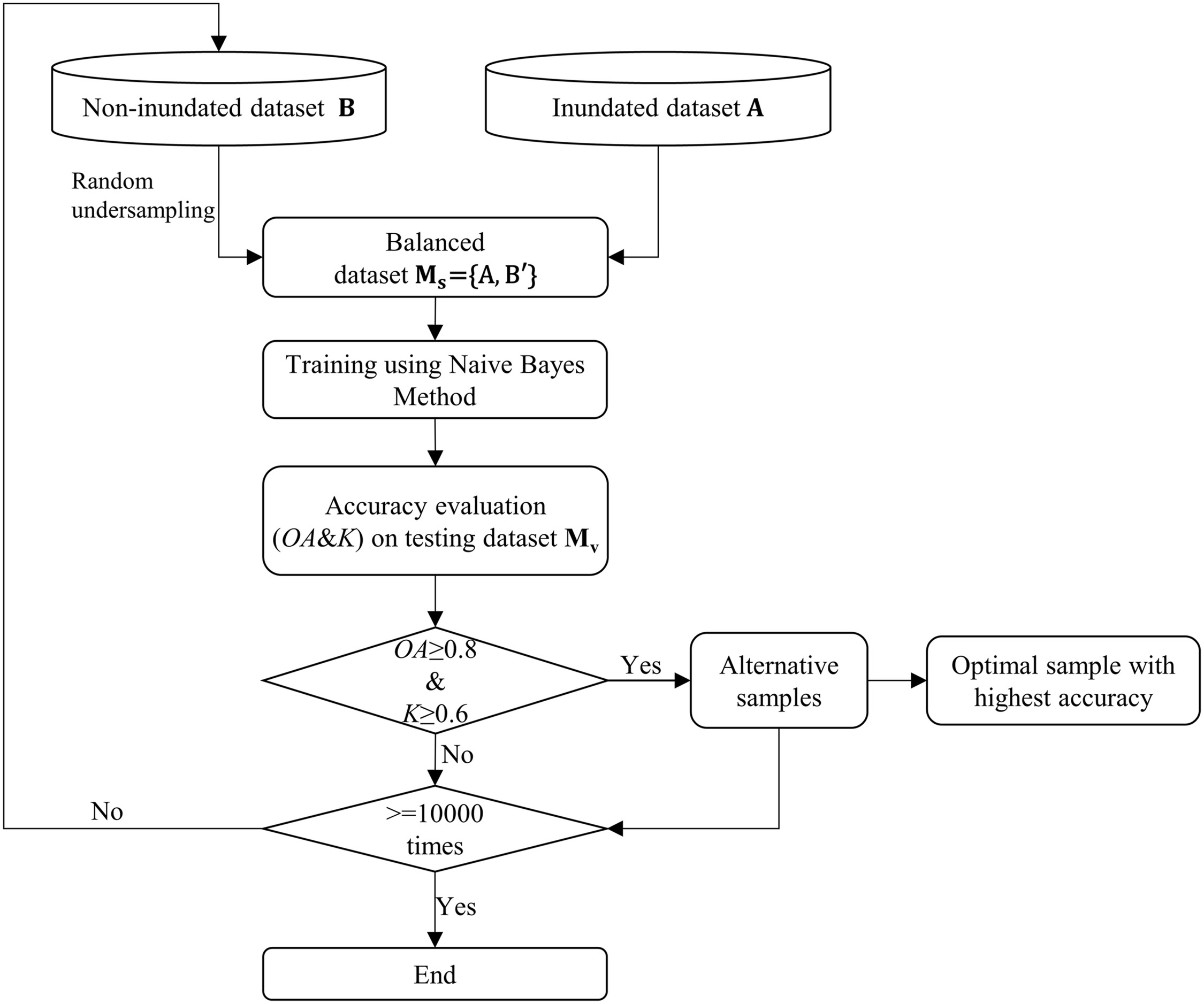
In regard to the evaluation metrics, the overall accuracy (OA) and Cohen’s kappa coefficient () are adopted to quantify the classification performance. OA is computed as the ratio between the number of correctly classified test samples and the total test samples. is considered to assess the extent of agreement between the prediction results and the actual classification results. An OA value that exceeds 0.8 indicates good classification accuracy. A value greater than 0.6 indicates that a given classification is unlikely to have been obtained by chance alone.
If the samples pass the relevant OA and thresholds, they are stored as alternative sampling tables. The random undersampling process is repeated 10,000 times to ensure that the probability distribution of each factor is infinitely close to the actual probability distribution. The most accurate table is selected as the optimal sample through accuracy comparison.
Probability Assessment Based on the Naïve Bayesian Model
After acquiring the optimal sample, the posterior probabilities of inundation and noninundation in each grid can be calculated with Eqs. (2) and (3), respectivelywhere and = the prior probabilities of inundation and noninundation, respectively; and = inundation and noninundation, respectively; = the influencing factor; and and = the conditional probabilities of each influencing factor under inundation condition and noninundation condition, respectively.
(2)
(3)
The posterior probability is the revised or updated probability of an event occurring after taking into consideration new information. Although the posterior probabilities are biased due to a change in the priors, undersampling does not affect the ranking order returned by the posterior probability (Pozzolo et al. 2015). In order to analyze the inundation risk, a standardized probability () of posterior inundation probability in each spatial grid is calculated with Eq. (4)
(4)
The standardized probability ranges from 0 to 1 and is further divided into five levels at equal intervals: very low (); low (0.2–0.4); medium (0.4–0.6); high (0.6–0.8); and very high (), which indicates the flood inundation risk. Finally, probabilistic flood inundation maps are generated in five levels.
Sensitivity Analysis
A sensitivity analysis is performed to quantify the effect of each selected urban factor on the flood inundation probability. This analysis is achieved by investigating the effect of small changes in the influencing factor probability on the posterior probability. The derivative function is applied to identify and estimate the contribution of each factor to the overall probability (Laskey 1995). Specifically, GeNIe software (BayesFusion, LLC 2021) is adopted to calculate the factor sensitivity based on the algorithm proposed by Kjærulff and van der Gaag (2000). The specific process entails the acquisition of a set of target nodes and the application of a derivative function to calculate the complete derivative of the posterior probability distribution of the target node to each numerical parameter in the Bayesian model. The derivative functions are shown in Eqs. (5) and (6). The higher the sensitivity value is, the more pronounced the influence of the representative factor on the inundation probability (Wang et al. 2002)where = the probability of each influencing factor; = a query, i.e., inundation or noninundation; and = the evidence corresponding to the value of entered into the Bayes model, which is part of the influencing factors. Moreover, = the posterior probability, which is a fraction of two linear functions of ; = sensitivity value of query y at x given e; and , , , and = constants with respect to .
(5)
(6)
Study Area and Materials
Study Area
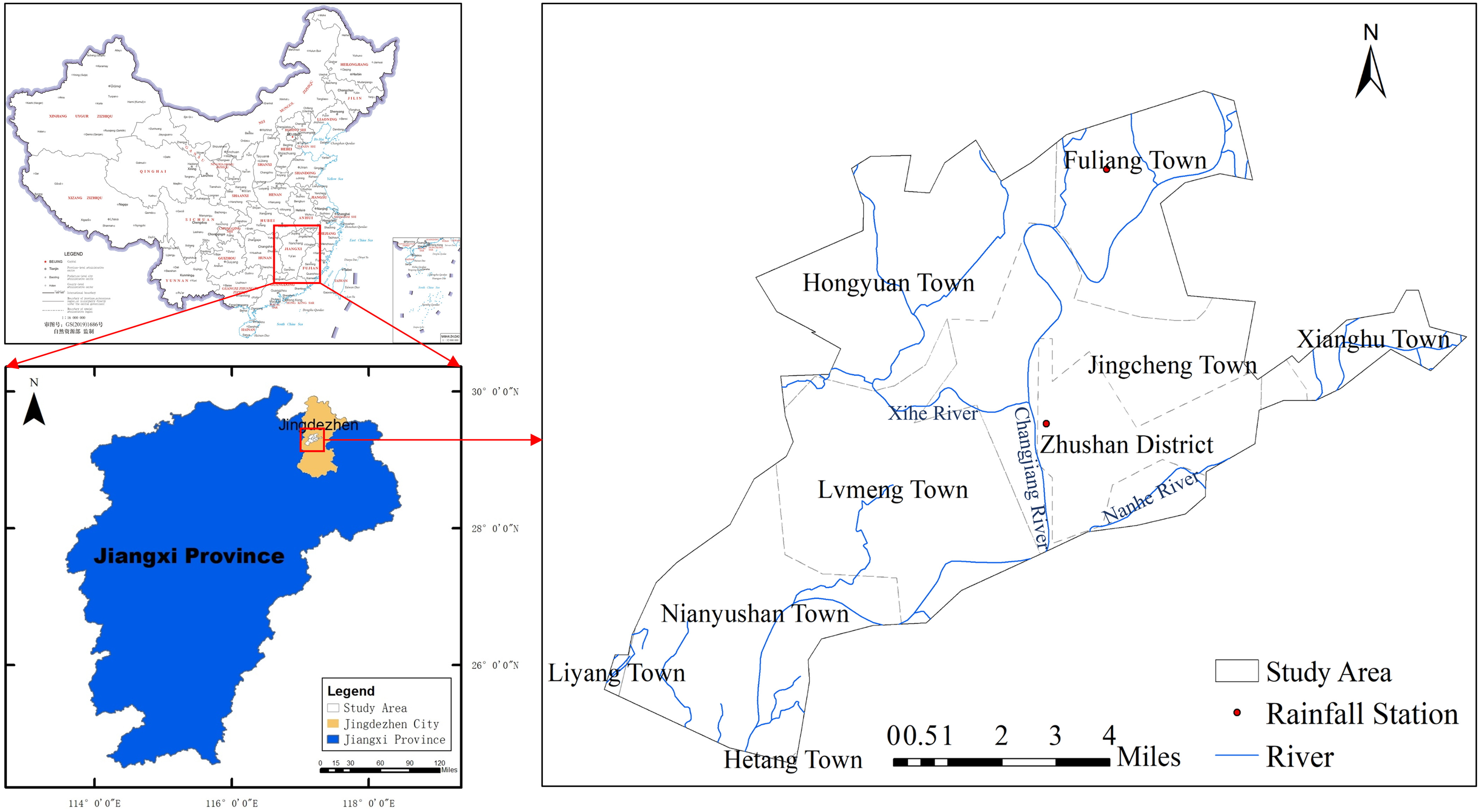
Jingdezhen City is located in northeastern Jiangxi Province, where the terrain is high in the boundary area and low at the center, similar to a basin. As one of the three major storm centers in Jiangxi Province, Jingdezhen City frequently and seriously suffers from severe floods resulting from sustained heavy rainfall, especially in low-lying areas along the river. On June 19, 2016, the entire city suffered severe flooding; the average rainfall was 240 mm. According to reports from the Jingdezhen Government, 375,000 people were affected, and the direct economic losses were 700 million Chinese Yuan. In the first 10 days of July 2020, the rainfall was 492 mm. Four consecutive flooding events occurred in Changjiang, thereby exceeding historical records. The hydrographic bureau issued red warnings many times during these events.
According to Master Plan of Jingdezhen (2012–2030), the central urban area of Jingdezhen, with an area of approximately , is selected as the study area [Fig. 4, released by Ministry of Natural Resources of the People’s Republic of China (2019)]. In this area, the population is concentrated, and the infrastructure, such as roads, drainage networks, water conservancy, and so on, is constructed. The average elevation is 32 m, and the terrain is inclined from northeast to southwest. There are nine administrative districts, including Liyang Town, Lvmeng Town, Hongyuan Town, Fuliang Town, Xianghu Town, Zhushan District, Jingcheng Town, Hetang Town, and Nianyushan Town. The Changjiang River and its tributaries, namely, the Nanhe River and Xihe River, flow through the central urban area.
Data Collection and Processing
Factors Selection and Data Collection
Urban floods are generally triggered by intense rainfalls when the capacity of urban drainage systems is overwhelmed (Chen et al. 2015). In this study, we assume that rainfall is evenly distributed in space because the study area is a small region. Besides the rainfall, underlying surface factors such as urban drainage systems, hydrology (river network), soils and land cover (soil water retention capacity), and topography (elevation and slope) interactively influence and control the dynamic processes of flooding, according to previous studies (Liu et al. 2016; Abebe et al. 2018; Wu et al. 2019, 2021). Moreover, with rapid and large-scale urbanization, much of the land surface is now covered by roads and buildings. These roads and buildings are impervious, which reduce infiltration of water into the ground and accelerate runoff to ditches and streams. Therefore, flood disasters are also associate with road density (Rahman et al. 2021).
In conclusion, the spatial differences in topographic characteristics, soil conditions, river network, drainage networks, and road networks affect urban flood inundation probability significantly. Taking the characteristics of the study area into account, elevation, slope, soil water retention (SWR), river network density and proximity, drainage network density, and road network density are identified as main influencing factors in this study.
Topographic Characteristics
It is pointed out that elevation and slope determine runoff formation time and its volume (Liu et al. 2020). Elevation data are collected from the Water Conservancy Bureau of Jingdezhen City, and slope data are extracted from a digital elevation model (DEM) to quantify the control of the topography of the hydrological process. The DEM and slope are shown in Figs. 5(a and b), respectively.

SWR
The potential maximum SWR is considered to reflect the ability of soil to relieve rainfall pressure, which is related to urban flood disasters. According to the Soil Conservation Service curve number (SCS CN) method, the potential maximum SWR can be calculated through . The curve number (CN) value is determined by the infiltration capacity of the land cover type in each grid unit and the soil type to which it belongs. Referring to Tang et al. (2018), the hydrologic soil groups were classified into four groups (A, B, C, and D) determined by the infiltration rate of each soil (see Table 1). CN values are summarized in Table 2 based on the combinations of infiltration rates of soil and land cover in the study area. The potential maximum SWR in the study area is shown in Fig. 5(c).
| HSG | Soil texture | Infiltration rate |
|---|---|---|
| A | Sand, loamy sand, sandy soil | Highest |
| B | Loam, silty loam | High |
| C | Sandy clay loam | Low |
| D | Clay loam, silty clay loam, sandy clay, silty clay, clay | Minimum |
| Land cover category | Hydrologic soil group | |||
|---|---|---|---|---|
| A | B | C | D | |
| Evergreen broadleaf forest | 25 | 55 | 70 | 77 |
| Evergreen needleleaf forest | 25 | 55 | 70 | 77 |
| Mixed forest | 36 | 60 | 73 | 79 |
| Second forest | 32 | 58 | 72 | 79 |
| Barren | 78 | 82 | 88 | 90 |
| Shrub | 45 | 66 | 83 | 83 |
| Grass | 34 | 60 | 74 | 80 |
| Orchard | 40 | 62 | 76 | 82 |
| Wetland | 72 | 82 | 88 | 90 |
| Low-density residential | 48 | 66 | 78 | 83 |
| High-density residential | 77 | 85 | 90 | 92 |
| Commercial/industrial | 89 | 92 | 94 | 95 |
| Cropland | 58 | 72 | 81 | 85 |
| Water | 100 | 100 | 100 | 100 |
River Network and Proximity
River network map data were collected from the National Basic Geographic Information Centre (2017). The river network density refers to the river length per unit area and is calculated with a linear density function for a radius of 1 km. River proximity reflects the distance to the river, which can be obtained using a multiple buffer tool. The river proximity and river network density in the study area are shown in Figs. 5(d and e), respectively.
Drainage and Road Networks
The urban drainage network expresses the water volume that the system can accommodate. Road network density influences runoff and drainage in a floodplain. Drainage and road network data were obtained from the Water Resources Bureau of Jingdezhen City. The drainage and road network densities are calculated using the linear density function with a radius of 1 km. The drainage network density and road density are shown in Figs. 5(f and g), respectively.
Inundation Maps for Different Return Periods
Inundation maps for different return periods were collected from the Development of a Master Plan for Jingdezhen City Integrated Flood Risk Management Consulting Services (Wang et al. 2015a), which implemented the Jiangxi Wuxikou Integrated Flood Management Project.
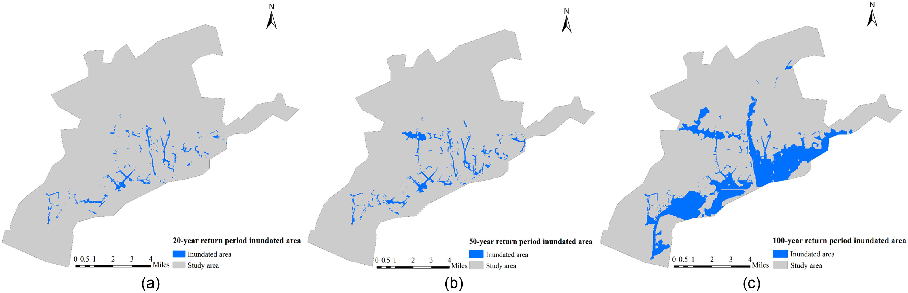
The spatial distribution of inundation areas for 20-, 50-, and 100-year return periods is collected at a 30 m spatial resolution (Pregnolato et al. 2021), as shown in Fig. 6. The results are produced via Danish Hydraulic Institute (DHI) MIKE modeling under current conditions and apply the design rainstorm and flood (considering different return periods) inferred by a typical flood in 1998 as input. The daily precipitations are 261.1, 311.5, and 349.0 mm for 20-, 50-, and 100-year return periods, respectively. River flooding and urban-area waterlogging are considered in the simulation process. The model encompasses a coupling simulation of an urban drainage network model, river model, and 2D surface flow model. In this study, the number of submerged grids in the 20-year return period is 3,425; the number of submerged grids in the 50-year return period is 5,693; and the number of submerged grids in the 100-year return period is 33,832.
Data Processing
There are two types of influencing factors: raster data, including soil type, land use data, and the DEM; and vector data, such as the area boundary and river, road, and drainage networks. The spatial resolution is set to 30 m, and 213,540 grids are established in the study area.
To facilitate Bayesian model processing, all variables should be unified considering classification standards. Regarding inundation maps, 0 indicates noninundated areas, and 1 indicates inundated area. In regard to the influencing factors, the value of each factor is divided into five classes based on expert suggestions and relevant studies (Huang et al. 2021), of which 1 indicates the lowest class and 5 indicates the highest class (as summarized in Table 3). The spatial distributions of the seven factors are shown in Fig. 5.
| Class | Influencing factors | ||||||
|---|---|---|---|---|---|---|---|
| Elevation (m) | Slope (%) | SWR (mm) | River density () | River proximity (m) | Pipe density () | Road density () | |
| Very low | |||||||
| Low | 30–50 | 1–5 | 40–80 | 0.1–0.6 | 200–400 | 0.5–2 | 2–4 |
| Medium | 50–70 | 5–10 | 80–120 | 0.6–1.2 | 400–600 | 2–3.5 | 4–6 |
| High | 70–90 | 10–15 | 120–160 | 1.2–1.8 | 600–800 | 3.5–5 | 6–8 |
| Very high | |||||||
Results
Optimal Sample for the Different Flood Return Periods
Optimal samples (Table 4) are selected from all sampling tables, satisfying the accuracy requirements after 10,000 training epochs. The sample numbers of the inundated and noninundated grids in the optimal sample for the 20-, 50-, and 100-year return periods are 3,425, 5,693, and 33,832, respectively. The OA index and index meet the aforementioned requirements, with values greater than 0.8 and 0.6, respectively.
| Return period (year) | Sample number of inundated grids | Sample number of noninundated grids | OA | K |
|---|---|---|---|---|
| 20 | 3,425 | 3,425 | 0.8693 | 0.7363 |
| 50 | 5,693 | 5,693 | 0.8489 | 0.6983 |
| 100 | 33,832 | 33,832 | 0.8790 | 0.7288 |
Based on the selected optimal sample, the prior and conditional probabilities are calculated. The conditional probability distribution is the distribution of each factor at different levels under inundation and noninundation conditions, from which it is determined that the distribution of each influencing factor under inundation conditions is completely different from that under noninundation conditions. For example, Fig. 7 shows the prior and conditional probabilities that correspond to the optimal sample for the 100-year return period. The conditional probability of elevation with Class 1 under inundation conditions is high, but it is very low under noninundation conditions. Similar results are observed for the 20- and 50-year return periods but are not repeated here.

Inundation Probability Maps
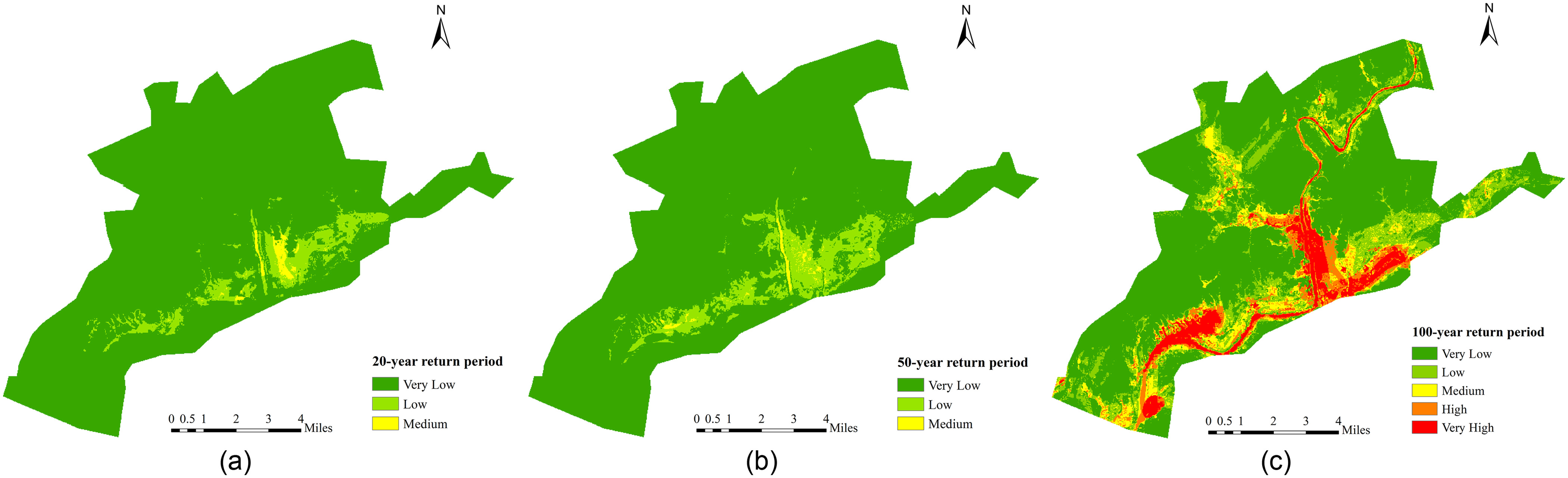
Based on the trained results of the prior and conditional probabilities, the posterior probability for each grid is calculated. Flood inundation probability maps of Jingdezhen Central City based on the proposed method for the 20-, 50-, and 100-year return periods are shown in Fig. 8.

From the 20- to 100-year return periods, the flood inundation probability distinctly increases. Statistics of the spatial inundation probability are shown in Table 5. The average inundation probability increases from 0.2190 to 0.3828. Areas with a high probability also increase, e.g., certain areas with a moderate probability for the 20- and 50-year return periods attain a high probability for the 100-year return period. The proportions of the areas with a moderate or higher probability for the 20-, 50-, and 100-year return periods are 24.5%, 28.7%, and 42.2%, respectively.
| Return period (year) | Mean | Maximum | Percentage of areas with moderate above probability (%) |
|---|---|---|---|
| 20 | 0.2190 | 0.9851 | 24.5 |
| 50 | 0.2809 | 0.9861 | 28.7 |
| 100 | 0.3828 | 1.0000 | 42.2 |
The most obvious changes are observed on both sides of the Changjiang River. The most likely inundated areas are concentrated at the city center along the Changjiang River and extend in the east and west directions in the 20- and 50-year return periods. Compared with the 20-year return period, in the 50-year return period, the most likely inundated areas extend more widely to the east, west, and north, for which the observed extension is roughly consistent with the distribution of the river. The areas likely to be inundated further expand in the 100-year return period, for which the high-probability areas are located along the Changjiang River. The probability gradually decreases toward the surrounding areas. High-probability areas are concentrated in Zhushan District and Jingcheng Town along the Changjiang River. Fuliang Town, Hongyuan Town, Xianghu Town, and other areas transition from low-probability areas in the 20- and 50-year return periods to moderate- and high-probability areas in the 100-year return period.
There are obvious differences in the inundation probability among the various regions. Zhushan District exhibits the highest probability, followed by Nianyushan Town. The average probability of these two regions for the 100-year return period reaches 0.7758 and 0.4564, respectively. Areas with the highest probability are concentrated near the Changjiang River in Zhushan District, where impervious areas are increasing because of the area’s rapid economic development and increasing population density. In Nianyushan Town, areas with the highest probability are also located near the river.
The areas in Jingcheng Town along the Xihe River also attain high probabilities (the average probability is 0.3810), which are mainly attributed to the basin-shaped terrain with a higher elevation in the boundary region and a lower elevation at the center. Furthermore, the areas exhibit a high river density and are more likely to become flooded in the event of heavy rain.
The average probability in Lvmeng Town is 0.3500 in the 100-year return period. In addition to the areas near the river, high-probability areas are concentrated in the southern part of Lvmeng Town, which is an extremely low-lying region. The probability in Hongyuan Town and Fuliang Town is relatively low. The high-probability area in Liyang Town in the southwest region is large, but this area mainly comprises rural areas.
Results Verification
To verify the effectiveness of the proposed method in urban flood inundation probability assessment, grids with a moderate or higher probability in the different return periods are compared with the inundation maps produced via DHI MIKE modeling. The proportion of the consistent grids to the total inundated grids is calculated. Fig. 9 shows the prediction accuracy based on the naïve Bayes model with data reconstruction for the different return periods. Blue indicates the area that is consistent with the modeled inundation situation; red indicates the area that is inconsistent with the modeled inundation situation. The accuracy rates for the 20-, 50-, and 100-year return periods are 91.97%, 88.38%, and 88.79%, respectively, thereby demonstrating that the proposed model achieves good performance.

For comparison, the results are also obtained with the traditional naïve Bayes model without data reconstruction. The traditional method does not address the imbalance between inundation sample sets and noninundation sample sets. The results reveal that the traditional model does not pass the overall accuracy and Cohen’s kappa coefficient tests for all three return periods. The resultant flood inundation probability maps are shown in Fig. 10.
Compared with Fig. 8, the inundation probabilities depicted in Fig. 10 for the three return periods are highly underestimated. The areas that are most likely to be inundated are much smaller, especially for the 20- and 50-year return periods. As previously mentioned, when the sample distribution of the categories in the training set is uneven, the classifier substantially focuses on categories with larger sample sizes and disregards those with smaller sample sizes (Wickramasinghe and Kalutarage 2020).
Fig. 11 shows the prediction results based on the traditional Bayesian model for the three return periods. A statistical comparison between the traditional approach and the proposed method is carried out (Table 6). The accuracy of the naïve Bayes model without data reconstruction is 10.16%, 6.69%, and 66.21% for the 20-, 50-, and 100-year return periods, respectively, which is much lower than that of the naïve Bayes model with data reconstruction, at accuracies of 91.97%, 89.74%, and 90.6%, respectively. The results suggest that many inundated grids cannot be identified with the naïve Bayes classifier without data reconstruction. Moreover, the accuracy of the proposed model with data reconstruction is much higher, especially in the 20- and 50-year return periods, as the imbalance gaps are narrowed through data reconstruction, which can significantly improve the modeling accuracy.

| Model accuracy | 20 year (%) | 50 year (%) | 100 year (%) |
|---|---|---|---|
| Naïve Bayes model without data reconstruction | 10.16 | 6.69 | 66.21 |
| Naïve Bayes model with data reconstruction | 91.97 | 89.74 | 90.6 |
Sensitivity of the Influencing Factors
The sensitivity value of each selected urban influencing factor, which is calculated based on the mean probability in the three return periods, is listed in Table 7. The sensitivity of the different factors varies. The drainage network density exhibits the highest sensitivity value of 0.64, followed by the elevation with a sensitivity value of 0.46. In addition, the river density and slope exert great impacts on the inundation probability.
| Factors | Sensitivity value |
|---|---|
| Elevation | 0.46 |
| Slope | 0.27 |
| SWR | 0.13 |
| River density | 0.34 |
| River proximity | 0.13 |
| Drainage network density | 0.64 |
| Road density | 0.18 |
The higher the drainage network density is, the higher the inundation probability, as inundation is mostly caused by overflow of the drainage system in urban areas. The drainage network density is relatively high in the Zhushan District, Jingcheng, and Lvmeng, which are central areas of Jingdezhen City. The inundation probability is higher in these areas, as the drainage design standard is low, and most pipes were designed based on only a one-year return period. The elevation also imposes a notable influence on the inundation probability. Small elevation changes may cause large changes in the inundation probability. The lower the elevation is, the higher the inundation probability of an area. In Jingdezhen City, the terrain is complex and dips from northeast to southwest. Therefore, the elevation varies greatly. Low-lying areas located in the southwest are easily inundated and should be given more attention. In addition, the slope determines inundation. The steeper the slope is, the higher the water flow. The river density is also a sensitive influencing factor. In addition to the city center along the Changjiang River, areas with a higher river network density attain a high inundation probability.
The sensitivity of the river proximity is relatively low, but this finding does not suggest that river proximity is a nonessential factor. High-probability areas in the central city of Jingdezhen are concentrated near the river and extend toward surrounding areas. Under the dual influences of heavy rainfall and external floods, areas closer to the river are therefore more prone to flooding and inundation. The low sensitivity is mainly attributed to the overall high level in urban areas where the Changjiang River runs through. The same situation is also found in the road network density factor, which yields a minimal difference in this case. In addition, the probability of urban flood inundation is less sensitive to the potential maximum SWR in this study. This indicates that the changes in potential maximum SWR lead to fewer changes in the probability of urban flood inundation.
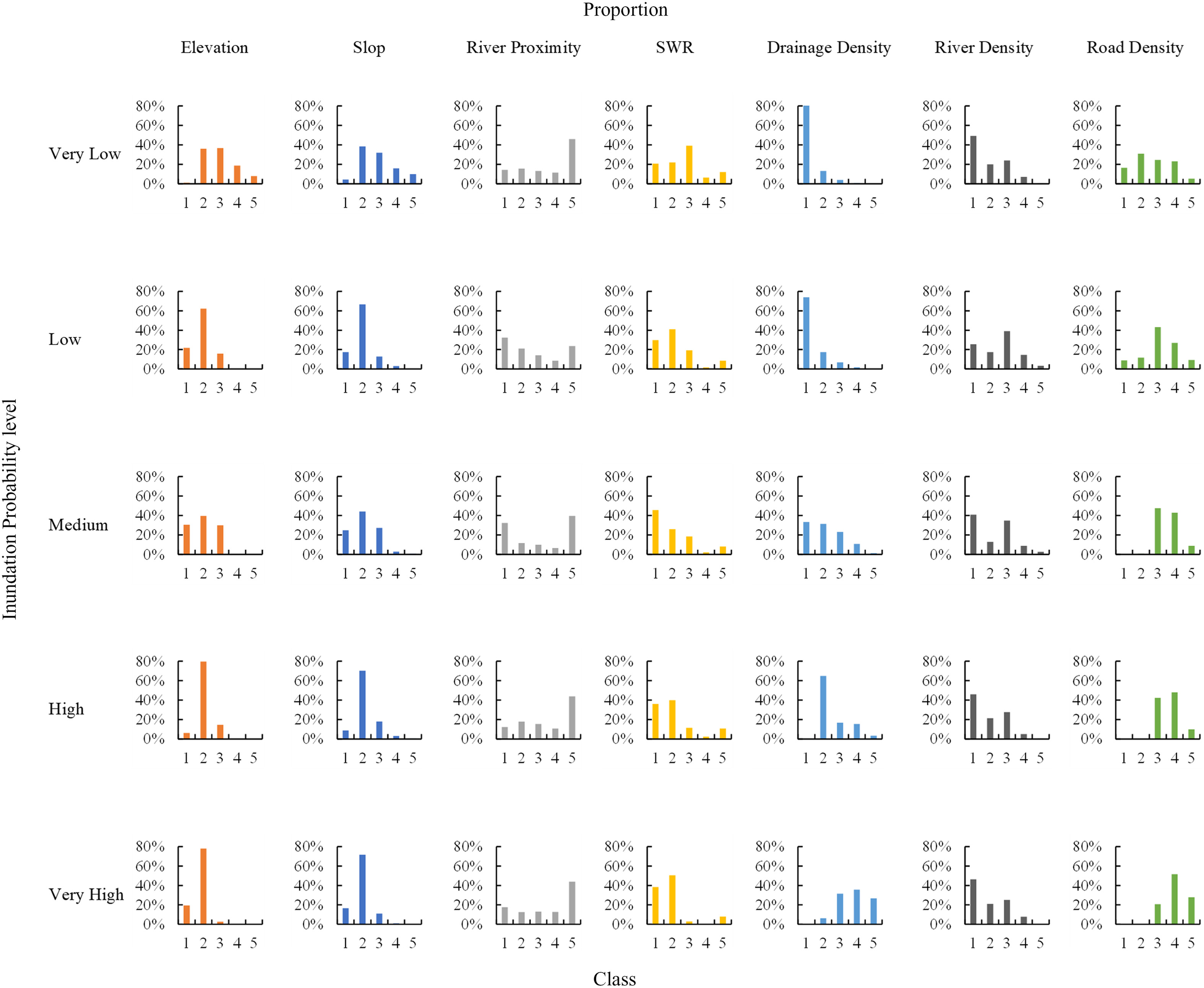
To further verify the sensitivity analysis results, statistical analysis of the distribution characteristics of the seven influencing factors is conducted at different probability levels in Fig. 12. The horizontal axis indicates the class of each factor, and the vertical axis indicates the proportion of the total grids at a given probability level. The class distribution of each factor at the different probability levels varies, thus revealing that changes in the drainage network density, elevation, slope, and river network density may cause great changes in the inundation probability. Specifically, the proportion of the drainage network density in Class 1 decreases with an increase in the inundation probability from very low to very high, while the proportions of the drainage network density in classes 4 and 5 exhibit the opposite trend (the proportions increase with an increase in the inundation probability). This finding indicates that the drainage density exerts a significant impact on the flood inundation probability. From very low to very high inundation probabilities, the mean proportion of the elevation at levels 3 to 5 decreases, and the mean proportion at levels 1 and 2 increases. This finding demonstrates that the lower the elevation is, the higher the inundation probability. The slope trend is consistent with that of the elevation, which is not unexpected, as the slope is highly relevant to elevation changes.
Discussion
In this paper, an improved Bayesian method through data reconstruction is proposed to assess the spatial inundation probability of urban floods under different return periods. The undersampling technique is used to reconstruct data before developing the Bayesian method, which can address the imbalance problem between inundation and noninundation data sets. However, some important samples from the majority class might be overlooked using the undersampling technique (Tang et al. 2018), which would result in overestimation of the inundation situation. Therefore, the -means clustering technique is used to divide noninundated grids into several equal groups based on the geographic location before random undersampling. This approach ensures that as many samples as possible can be collected from different geographic locations, thus reducing the risk of removing useful data from noninundation samples. As a result, the assessment accuracy of the proposed method is much higher than that based on the naïve Bayes model without data construction. Although grouping noninundated grids according to geographic locations is a simple method that achieves good performance, many different random undersampling methods could be explored in the future. For example, Bach and Werner (2021) proposed the KNN_RU method, which removes the maximum -nearest neighbors of the samples belonging to the majority class. Lin et al. (2017) considered a small number of cluster centers and their nearest neighbors to represent all data samples of the majority class based on a clustering technique.
In addition, flood inundation probability maps are obtained considering different flood return periods. In previous studies, inundation data have often been derived via the superposition of different inundated surfaces during a given historical period, and a maximum inundation map has consequently been generated. Representative studies were developed by Liu et al. (2016, 2017) and Wu et al. (2019). However, the inundation probability of various areas differs. Certain areas may become inundated many times, while other areas may become inundated only once. Maximum inundation maps cannot distinguish this difference, which might over- or underestimate the inundation probability. The flood inundation probability maps generated in this study for different return periods can overcome this weakness and facilitate a more accurate probability assessment.
In our study, the influence of the urban environment on the probability of urban flood disaster risk is detected through sensitivity analysis. It is confirmed that both drainage network density and elevation are important factors for the probability of urban flood inundation. On a small scale, such as a 1 km resolution, topography and drainage mainly determine the inundation level (Chen et al. 2022). Because Jingdezhen City is located along the Changjiang River, fluvial floods also affect urban inundation. The areas with a higher river network density attain a high inundation probability. By contrast, potential maximum SWR is not a sensitive factor for the probability of urban flood inundation on a small scale, although it has an important impact on the flood runoff amount of the whole area (Szwagrzyk et al. 2018).
Conclusion
Urban floods cause unprecedented damage to lives and properties around world. An urban flood map is used to identify areas at risk of flooding and consequently to improve flood risk management and disaster preparedness. However, the spatial extent of flooding in urban areas is particularly uncertain. In order to quantify the uncertainty of urban flood inundation and explore the influence of the urban environment on the probability of urban flood disaster risk, a spatial inundation probability assessment model based on an improved naïve Bayesian model is proposed. First, data reconstruction through random undersampling before the naïve Bayesian model is conducted, and the -means clustering technique is adopted during undersampling. Second, flood inundation probability is calculated based on prior probability and conditional probability of each influencing factor. Last, sensitivity analysis is performed to identify the most contributed factor to the overall probability.
In conclusion, the findings of this study are presented as follows: (1) probabilistic inundation maps for different return periods are produced. Compared with the conventional maximum inundation mapping method, this study can more accurately calculate the inundation probability with greater detail for different return periods. (2) Data reconstruction through random undersampling before naïve Bayesian model application solves the imbalanced sample size problem, and the -means clustering technique ensures that as many samples as possible are collected from different geographic locations, thereby reducing the risk of removing useful data from noninundation samples. The inundation probability in the study area is more accurate than with the original naïve Bayesian model. The prediction accuracy reaches 91.97%, 89.74%, and 90.6% in the 20-, 50-, and 100-year return periods, respectively, in Jingdezhen. (3) The probability of urban flood inundation is sensitive to drainage network density and elevation in central Jingdezhen City.
The novelties of this study are mainly threefold. First, an improved naïve Bayesian method based on data reconstruction was proposed, which addressed the imbalanced problem and improved the accuracy of inundation probability. Second, urban flood inundation assessed using the Bayesian network is considered as an alternative to complex hydrological or hydrodynamic model simulations, which can quantify uncertainty and utilize available data and preexisting knowledge. Third, the inundation probabilities generated based on various return periods can provide more detailed inundation information than those determined with the commonly adopted superposition method, in which historical inundation maps are simply overlaid.
The proposed method is a simple and cost-effective way to obtain urban inundation probability compared with complex and costly hydrological or hydrodynamic model. More significantly, the inundation probability can be obtained rapidly and accurately without rebuilding and retraining the model once the environment is changed. Moreover, this method can be applied to other cities suffering from floods by establishing the relationship between spatial inundation and environmental factors. The model performance will be further improved with more historical data collected. Thus, our research is ongoing to verify this method by collecting more data from different cities in an attempt to establish a general and robust classifier that can be used anywhere and in the changing context.
Data Availability Statement
All data that support the findings of this study are available from the corresponding author upon reasonable request.
Acknowledgments
This research was funded by the National Natural Science Foundation of China, Award Nos. 42171081, 91846203, and 72174054. We would like to express our gratitude to the World Bank for the support to carry out the study, Loan No. 8237-CN, Project No. JDZ-WXK-ZX-9.
References
Abebe, Y., G. Kabir, and S. Tesfamariam. 2018. “Assessing urban areas vulnerability to pluvial flooding using GIS applications and Bayesian belief network model.” J. Cleaner Prod. 174 (Feb): 1629–1641. https://doi.org/10.1016/j.jclepro.2017.11.066.
Aridas, C. K., S. Karlos, V. G. Kanas, and S. B. Kotsiantis. 2019. “Uncertainty based under-sampling for learning naive Bayes classifiers under imbalanced data sets.” IEEE Access 8 (Dec): 2122–2133. https://doi.org/10.1109/ACCESS.2019.2961784.
Bach, M., and A. Werner. 2021. “Improvement of random undersampling to avoid excessive removal of points from a given area of the majority class.” In Proc., Int. Conf. on Computational Science, 172–186. Cham, Switzerland: Springer International Publishing.
Bajabaa, S., M. Masoud, and N. Al-Amri. 2013. “Flash flood hazard mapping based on quantitative hydrology, geomorphology and GIS techniques (case study of Wadi Al Lith, Saudi Arabia).” Arab. J. Geosci. 7 (6): 2469–2481. https://doi.org/10.1007/s12517-013-0941-2.
BayesFusion, LLC. 2021. “GeNIe.” Accessed September 15, 2021. https://www.bayesfusion.com/.
Chen, A. S., B. Evans, S. Djordjevic, and D. A. Savic. 2012. “Multi-layered coarse grid modelling in 2D urban flood simulations.” J. Hydrol. 470 (Nov): 1–11. https://doi.org/10.1016/j.jhydrol.2012.06.022.
Chen, Y., H. Hou, Y. Li, L. Wang, J. Fan, B. Wang, and T. Hu. 2022. “Urban inundation under different rainstorm scenarios in Lin’an City, China.” Int. J. Environ. Res. Public Health 19 (12): 7210. https://doi.org/10.3390/ijerph19127210.
Chen, Y., H. Zhou, H. Zhang, G. Du, and J. Zhou. 2015. “Urban flood risk warning under rapid urbanization.” Environ. Res. 139 (May): 3–10. https://doi.org/10.1016/j.envres.2015.02.028.
Cockburn, G., and S. Tesfamariam. 2012. “Earthquake disaster risk index for Canadian cities using Bayesian belief networks.” Georisk 6 (2): 128–140. https://doi.org/10.1080/17499518.2011.650147.
Di Baldassarre, G., G. Schumann, P. D. Bates, J. E. Freer, and K. J. Beven. 2010. “Flood-plain mapping: A critical discussion of deterministic and probabilistic approaches.” Hydrol. Sci. J. 55 (3): 364–376. https://doi.org/10.1080/02626661003683389.
Han, L., J. Zhang, Y. Zhang, Q. Ma, S. Alu, and Q. Lang. 2019. “Hazard assessment of earthquake disaster chains based on a Bayesian network model and ArcGIS.” ISPRS Int. Geo-Inf. 8 (5): 210. https://doi.org/10.3390/ijgi8050210.
Huang, S., H. Wang, Y. Xu, J. She, and J. Huang. 2021. “Key disaster-causing factors chains on urban flood risk based on Bayesian network.” Land 10 (2): 210. https://doi.org/10.3390/land10020210.
Jamali, B., R. Löwe, P. M. Bach, C. Urich, K. Arnbjerg-Nielsen, and A. Deletic. 2018. “A rapid urban flood inundation and damage assessment model.” J. Hydrol. 564 (Sep): 1085–1098. https://doi.org/10.1016/j.jhydrol.2018.07.064.
Kjærulff, U., and L. van der Gaag. 2000. “Making sensitivity analysis computationally efficient.” In Proc., 16th Annual Conf. on Uncertainty in Artificial Intelligence (UAI 2000). Cambridge, MA: Morgan Kaufmann.
Krawczyk, B. 2016. “Learning from imbalanced data: Open challenges and future directions.” Prog. Artif. Intell. 5 (4): 221–232. https://doi.org/10.1007/s13748-016-0094-0.
Laskey, K. B. 1995. “Sensitivity analysis for probability assessments in Bayesian networks.” IEEE Trans. Syst. Man Cybern. 25 (6): 901–909. https://doi.org/10.1109/21.384252.
Lee, S., M. Lee, H. Jung, and S. Lee. 2020. “Landslide susceptibility mapping using Naïve Bayes and Bayesian network models in Umyeonsan, Korea.” Geocarto Int. 35 (15): 1665–1679. https://doi.org/10.1080/10106049.2019.1585482.
Li, L., J. Wang, H. Leung, and C. Jiang. 2010. “Assessment of catastrophic risk using Bayesian network constructed from domain knowledge and spatial data.” Risk Anal. 30 (7): 1157–1175. https://doi.org/10.1111/j.1539-6924.2010.01429.x.
Liang, W., D. Zhuang, D. Jiang, J. Pan, and H. Ren. 2012. “Assessment of debris flow hazards using a Bayesian network.” Geomorphology 171 (Oct): 94–100. https://doi.org/10.1016/j.geomorph.2012.05.008.
Lin, W. C., C. F. Tsai, Y. H. Hu, and J. S. Jhang. 2017. “Clustering-based undersampling in class-imbalanced data.” Inf. Sci. 409 (Oct): 17–26. https://doi.org/10.1016/j.ins.2017.05.008.
Liu, R., Y. Chen, J. Wu, L. Gao, D. Barrett, T. Xu, L. Li, C. Huang, and J. Yu. 2016. “Assessing spatial likelihood of flooding hazard using naïve Bayes and GIS: A case study in Bowen Basin, Australia.” Stochastic Environ. Res. Risk Assess. 30 (6): 1575–1590. https://doi.org/10.1007/s00477-015-1198-y.
Liu, R., Y. Chen, J. Wu, L. Gao, D. Barrett, T. Xu, L. Li, C. Huang, and J. Yu. 2017. “Integrating entropy-based naive Bayes and GIS for spatial evaluation of flood hazard.” Risk Anal. 37 (4): 756–773. https://doi.org/10.1111/risa.12698.
Liu, Y., X. Lu, Y. Yao, N. Wang, Y. Guo, C. Ji, and J. Xu. 2020. “Mapping the risk zoning of storm flood disaster based on heterogeneous data and a machine learning algorithm in Xinjiang, China.” J. Flood Risk Manage. 14 (1): e12671. https://doi.org/10.1111/jfr3.12671.
Merwade, V., F. Olivera, M. Arabi, and S. Edleman. 2008. “Uncertainty in flood inundation mapping: Current issues and future directions.” J. Hydrol. Eng. 13 (7): 608–620. https://doi.org/10.1061/(ASCE)1084-0699(2008)13:7(608).
Ministry of Natural Resources of the People’s Republic of China. 2019. “Map of China [Map].” Accessed July 21, 2022. http://bzdt.ch.mnr.gov.cn/.
Mohammed, R., J. Rawashdeh, and M. Abdullah. 2020. “Machine learning with oversampling and under sampling techniques: Overview study and experimental results.” In Proc., 2020 11th Int. Conf. on Information and Communication Systems (ICICS). New York: IEEE.
National Basic Geographic Information Centre. 2017. “1:250,000 National basic geographic database.” Accessed September 20, 2022. https://www.webmap.cn/commres.do?method=result25W.
Pozzolo, A. D., O. Caelen, R. A. Johnson, and G. Bontempi. 2015. “Calibrating probability with undersampling for unbalanced classification.” In Proc., 2015 IEEE Symp. Series on Computational Intelligence, 159–166. New York: IEEE.
Pregnolato, M., D. Han, A. L. Jacomo, R. D. Risi, J. Agarwal, and J. Huang. 2021. “Resilient infrastructures for reducing urban flooding risks.” In Water-wise cities and sustainable water systems: Concepts, technologies, and applications, edited by X. C. Wang and G. Fu. London: IWA Publishing.
Rahman, M., et al. 2021. “Flooding and its relationship with land cover change, population growth, and road density.” Geosci. Front. 12 (6): 101224. https://doi.org/10.1016/j.gsf.2021.101224.
Sevinc, V., O. Kucuk, and M. Goltas. 2020. “A Bayesian network model for prediction and analysis of possible forest fire causes.” For. Ecol. Manage. 457 (Feb): 117723. https://doi.org/10.1016/j.foreco.2019.117723.
Sun, R., G. Gao, Z. Gong, and J. Wu. 2020. “A review of risk analysis methods for natural disasters.” Nat. Hazards 100 (2): 571–593. https://doi.org/10.1007/s11069-019-03826-7.
Szwagrzyk, M., D. Kaim, B. Price, A. Wypych, E. Grabska, and J. Kozak. 2018. “Impact of forecasted land use changes on flood risk in the Polish Carpathians.” Nat. Hazards 94 (1): 227–240. https://doi.org/10.1007/s11069-018-3384-y.
Tang, X., Y. Shu, Y. Lian, Y. Zhao, and Y. Fu. 2018. “A spatial assessment of urban waterlogging risk based on a weighted naïve Bayes classifier.” Sci. Total Environ. 630 (Mar): 264–274. https://doi.org/10.1016/j.scitotenv.2018.02.172.
UNISDR (United Nations Office for Disaster Risk Reduction). 2009. Terminology on disaster risk reduction. Geneva: UNISDR.
Wang, H., I. Rish, and S. Ma. 2002. “Using sensitivity analysis for selective parameter update in Bayesian network learning.” In Proc., AAAI Spring Symp. on Information Refinement and Revision for Decision Making: Modeling for Diagnostics, Prognostics and Prediction. Reston, VA: American Institute of Aeronautics and Astronautics.
Wang, H., H. Zhang, Z. Liang, G. Li, Q. Lu, J. Huang, and D. Sun. 2015a. Consulting services for: Development of master plan for Jingdezhen City integrated flood risk management. Nanjing, China: Hohai Univ.
Wang, Z., C. Lai, X. Chen, B. Yang, S. Zhao, and X. Bai. 2015b. “Flood hazard risk assessment model based on random forest.” J. Hydrol. 527 (Aug): 1130–1141. https://doi.org/10.1016/j.jhydrol.2015.06.008.
Wickramasinghe, I., and H. Kalutarage. 2020. “Naive Bayes: Applications, variations and vulnerabilities: A review of literature with code snippets for implementation.” Soft Comput. 25 (3): 2277–2293. https://doi.org/10.1007/s00500-020-05297-6.
Wu, M., Z. Wu, W. Ge, H. Wang, Y. Shen, and M. Jiang. 2021. “Identification of sensitivity indicators of urban rainstorm flood disasters: A case study in China.” J. Hydrol. 599 (Aug): 126393. https://doi.org/10.1016/j.jhydrol.2021.126393.
Wu, Z., Y. Shen, H. Wang, and M. Wu. 2019. “Assessing urban flood disaster risk using Bayesian network model and GIS applications.” Geomatics Nat. Hazards Risk 10 (1): 2163–2184. https://doi.org/10.1080/19475705.2019.1685010.
Information & Authors
Information
Published In

Natural Hazards Review
Volume 24 • Issue 4 • November 2023
Copyright
This work is made available under the terms of the Creative Commons Attribution 4.0 International license, https://creativecommons.org/licenses/by/4.0/.
History
Received: Aug 5, 2022
Accepted: Mar 2, 2023
Published online: Aug 25, 2023
Published in print: Nov 1, 2023
Discussion open until: Jan 25, 2024
ASCE Technical Topics:
- Analysis (by type)
- Bayesian analysis
- Case studies
- Construction engineering
- Construction management
- Engineering fundamentals
- Floods
- Hydrologic data
- Hydrologic engineering
- Hydrology
- Infrastructure
- Mathematics
- Methodology (by type)
- Model accuracy
- Models (by type)
- Probability
- Research methods (by type)
- Statistical analysis (by type)
- Urban and regional development
- Urban areas
- Water and water resources
Authors
Metrics & Citations
Metrics
Citations
Download citation
If you have the appropriate software installed, you can download article citation data to the citation manager of your choice. Simply select your manager software from the list below and click Download.