Calibration of Frequency-Dependent Wave Speed and Attenuation in Water Pipes Using a Dual-Sensor and Paired-IRF Approach
Publication: Journal of Water Resources Planning and Management
Volume 150, Issue 11
Abstract
The propagation of pressure waves in water pipes is frequency dependent, which leads to these waves experiencing a frequency-dependent wave speed and attenuation, resulting in wave dissipation and dispersion. The effect is much more significant and complex in plastic pipes than in metal pipes, which makes most wave-based pipe condition assessment techniques ineffective for plastic pipes. In this paper, a new technique is developed to calibrate the frequency-dependent wave speed and attenuation for pressurized water pipes. Persistent hydraulic waves induced by a side-discharge valve are used as excitation. Pressure responses are measured using two pressure sensors, and a paired-impulse response function (paired-IRF) is determined through a deconvolution process. The transfer function between the two sensors is determined using the main spike in the paired-IRF trace, which contains the information on the wave propagation characteristics. The frequency-dependent wave speed and attenuation are then derived from the transfer function. The proposed new technique is validated by both numerical simulations and laboratory experiments. Three pipe configurations are considered in the experiments: (1) a high-density polyethylene (HDPE) pipe in the air; (2) an HDPE pipe buried in sand; and (3) a copper pipe in the air. The frequency-dependent wave speed and attenuation are calibrated for all three configurations and the results are distinctive from each other.
Introduction
Classic one-dimensional hydraulic transient (water hammer) theory (Wylie and Streeter 1993) has been applied to water pipes (e.g., concrete and metal pipes) for decades with assumed constant wave speed values. Based on the theory, a number of transient-based pipe condition assessment techniques have been developed (Brunone 1999; Duan 2016; Zeng et al. 2018; Wang et al. 2020; Zecchin et al. 2022; Ayati and Haghighi 2023). However, both laboratory (Bergant et al. 2008) and field results (Tijsseling et al. 2006; Stephens et al. 2011) illustrate that wave speed in water pipes is frequency-dependent, and hydraulic transient pressure waves experience not only dissipation but also dispersion. The dissipation and dispersion of hydraulic transient pressure waves is more significant and complex in viscoelastic pipes (e.g., plastic pipes) than in elastic pipes (e.g., metal pipes). This has impeded the effective application of transient-based condition assessment to plastic water pipes.
During hydraulic transient events, viscoelastic behavior and unsteady friction are important factors ascribed to the wave dissipation and dispersion (Gong et al. 2016b). In general, the impact of unsteady friction on the dissipation and dispersion of transient pressure waves is much less than that caused by the viscoelasticity (Covas et al. 2005). Therefore, the effect of unsteady friction is typically neglected when analyzing transient responses in short time frames (within seconds). The viscoelastic behavior of plastic pipes can be described by an instantaneous elastic strain followed by a gradual retarded strain for an applied load. Wave dissipation and dispersion in plastic pipes have been experimentally observed by several researchers in single pipe systems (Fox and Stepnewski 1974; Mitosek and Roszkowski 1998; Covas et al. 2004) and branched pipe systems (Evangelista et al. 2015). Several researchers proposed mathematical models to describe pressure dissipation and dispersion during hydraulic events with the use of a generalized Kelvin–Voigt (KV) mechanical model (Gally et al. 1979; Covas et al. 2004, 2005; Landry et al. 2012; Abdel-Gawad and Djebedjian 2020).
The KV model is a phenomenological model, and the model parameters need to be calibrated. Time-domain inverse transient analysis is a commonly used technique for the calibration (Covas et al. 2005; Soares et al. 2008; Covas and Ramos 2010; Duan et al. 2010; Meniconi et al. 2012; Pezzinga et al. 2014); however, the technique can only be applied to simple pipe configurations with known boundary conditions (e.g., reservoir–pipe–valve or reservoir–pipe–reservoir configurations). Recent studies used the frequency response function of the pipe system (as extracted by hydraulic trainset tests) for the KV parameter calibration (Gong et al. 2016b). However, it is also limited to simple pipe configurations for which the frequency response function can be analytically derived.
In addition to hydraulic transient waves, acoustic waves have also been used for condition assessment in water pipes (Hunaidi and Chu 1999; Brennan et al. 2007; Stephens et al. 2020). Acoustic waves are typically generated by introducing vibrations on the pipe wall or discharging water through a leak, and measured by accelerometers or hydrophones. In general, acoustic waves are typically much smaller in amplitude but higher in frequency than conventional hydraulic transient pressure waves. Previous research has shown that acoustic wave propagation in plastic pipes is highly dependent on the pipe wall, contained fluid and surrounding medium; therefore, wave speed and attenuation are difficult to predict in plastic pipes (Hunaidi and Chu 1999; Gao et al. 2017).
Several researchers have developed techniques to determine the frequency-dependent wave propagation characteristics for acoustic waves. Wavenumber is a commonly used parameter in acoustics, which includes the information of frequency-dependent wave speed and attenuation. Muggleton et al. (2002) developed the analytical equations to calculate the wavenumber for fluid-filled viscoelastic pipes surrounded by an infinite elastic medium. Experimental studies were conducted to validate the theoretical equation using three equally spaced sensors on a medium-density polyethylene (MDPE) pipe (Muggleton et al. 2004). Later, a transfer function method was used in an experimental study by Prek (2007). In that study, the transfer function was determined using three equally spaced hydrophones in a pipe. An extension of this work was conducted by Muggleton and Yan (2013) with consideration of the full three-dimensional effect of soil on a buried fluid-filled pipe. The measured wave speed and attenuation from experiments showed good agreement with the results from the modified theoretical equation. Recently, Gao et al. (2017) extended the work by considering the loading effect of three different surrounding mediums (air, water, and buried in sandy soil).
The aforementioned techniques reviewed require the use of three sensors equally spaced along the pipe. In real water distribution systems (WDSs), where most pipes are buried, it is difficult to have three locations equally spaced to install sensors. Although a two-sensor method has been mentioned in the literature with acoustic signal processing (Muggleton et al. 2004; Gao et al. 2005), it has limitations on its use with an assumption of negligible returning waves from system boundaries or any physical discontinuities. This assumption is only valid for waves with very small amplitude propagating in long and uniform water pipes, such that the wave is damped out due to energy losses as it propagates toward the boundary. This is difficult to achieve in urban pipe networks, where each pipe section is limited in length and reflections from the pipe cross-connections can be strong.
In the research reported in this paper, to overcome the limitations of existing techniques, a new nondestructive technique is developed to calibrate the frequency-dependent wave speed and attenuation (therefore, wave dissipation and dispersion). This is achieved by using two pressure sensors for measurement and analyzing a paired-impulse response function (paired-IRF). A unique benefit of using two sensors and the paired-IRF is that the transfer function of the target pipe section can be determined in complex pipe network environments (i.e., not affected by complex wave reflections, overcoming a key limitation of existing techniques). Numerical simulations are conducted to validate the proposed technique. The frequency-dependent wave speed and attenuation are determined from simulated pressure responses and the results are consistent with the theoretical values used in the numerical model. The technique is also validated through experimental studies on three pipe configurations: (1) a high-density polyethylene (HDPE) pipe anchored throughout and in the air; (2) an HDPE pipe anchored throughout and buried in sand; and (3) a copper pipe anchored throughout and in the air. The frequency-dependent wave speed and attenuation are calibrated for all the three configurations and the results are distinctive from each other.
Methodology
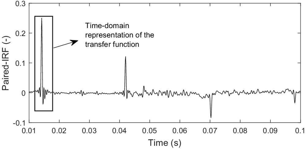
The development is built on a paired-IRF method originally developed by Zeng et al. (2020a) for leak detection in metallic pipes. Instead of analyzing the small perturbations in the paired-IRF trace that correspond to reflections from anomalies as in the previous work, the current research focus on the analysis of the main spike at the beginning of the paired-IRF that corresponds to the time-domain representation of the transfer function of the pipe section in-between the two sensors. The transfer function describes how a pressure wave propagates from one sensor to another, and it includes the information of wave dissipation and dispersion. In the current research, the approach for extracting the paired-IRF from a pipeline is the same, but the analysis of the paired-IRF is different.
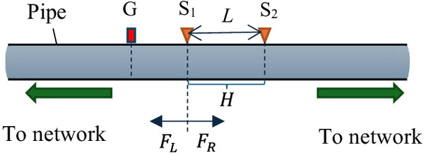
Fig. 1 shows the system configuration for implementing the technique. Any persistent pressure wave with good signal-to-noise ratio (typically an amplitude of 0.1 m or higher in water networks) and a wide bandwidth (up to hundreds of Hz or higher) will be suitable as excitation. The wave generator (G in Fig. 1) can be a partially open side-discharge valve, where the pulsating pressures are generated due to the turbulent flow around and through the valve. The nature of the pressure waves generated is similar to leak noise, but by using a partially open side-discharge valve, the pressure waves generated can be much larger in amplitude than typical leak noise. Two pressure sensors are used ( and , apart with a distance of ) to measure the pressure responses.
Original research by Zeng et al. (2020a) has discovered that, in the frequency domain, the ratio of the two pressure measurements (, where is the frequency-domain representation of the measured pressure and the subscript denotes the sensor location) is related to the transfer function () of the pipe section between the two sensors and the frequency response function (FRF) of the pipe system on one side of sensor , as shown in Eq. (1)where represents the FRF for the pipe system on the right-hand side of sensor , and denotes higher-order terms that can be neglected due to the small value. Once the ratio of is transformed from the frequency domain to the time domain, the result is termed “paired-IRF,” because it relates to the time-domain representation of .
(1)
In this research, the focus will be the transfer function (), which describes how a pressure wave propagates from to . Provided that the condition of the pipe section between to is uniform or changes in condition, if any, are minor (such that any reflections are much smaller than the incident wave), the time-domain representation of is the first perturbation in the paired-IRF trace (as highlighted in Fig. 5 later in the numerical study). As a result, the transfer function can be extracted from the paired-IRF trace in the time domain without knowing . Under the linear time-invariant (LTI) system theory, the frequency response function (FRF) of an LTI system is the Fourier transform of the system’s IRF (Che et al. 2021). The extracted first perturbation in the paired-IRF trace can be then converted to the frequency-domain transfer function [] through the Fourier transform.
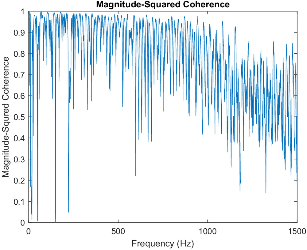
To ensure confidence in the determined transfer function, magnitude-squared coherence should be calculated for the measured pressures from the two sensors. The coherence value always ranges between 0 and 1, and it represents how a pair of signals are statistically related (with higher value representing higher causality between the two signals). Accurate determination of the transfer function is expected if the coherence value is close to 1. In order to remove the influence of interference and noise (which would result in low coherence), filters can be used to preprocess the pressure measurements.
Using the concept of complex wave number as borrowed from acoustics (Prek 2007), the transfer function for the pipe section between the two sensors can be expressed using Eq. (2)where is the complex wave number, is the imaginary unit, and is angular frequency. The real and imaginary part of relates to the frequency-dependent wave speed and attenuation coefficient , respectively (Prek 2007), as shown in Eqs. (3) and (4)
(2)
(3)
(4)
From the determined transfer function through the paired-IRF, the real part of the wave number can be determined. For wave components of which the half wavelength is less than the distance , the results need to be “unwrapped” (Muggleton et al. 2004; Prek 2007) because any value exceeding the range [] will be wrapped within the range [] when it is returned by the arctangent function. The unwrapped results are shown in Eq. (5) (Muggleton et al. 2004)where represents the argument (phase) of the transfer function , and is the number of half wavelengths between the two adjacent transducers. The unwrapped is then used to calculate the frequency-dependent wave speed through the use of Eq. (3).
(5)
The imaginary part of the wave number can also be determined from the transfer function. The unwrapped results are
(6)
Numerical Validation
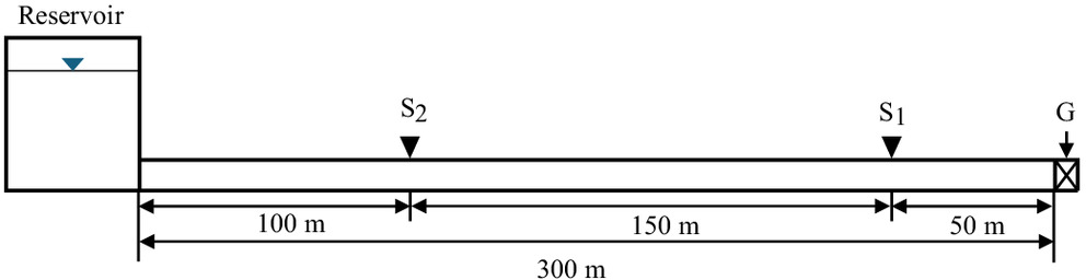
A simple reservoir–pipeline–valve system is used in this section to validate the proposed new technique for calibrating the frequency-dependent wave speed and attenuation. As shown in Fig. 2, this system contains a reservoir at the upstream end, a 300-m-long plastic pipe (viscoelastic pipe), and a valve at the downstream end. The internal diameter of the pipe is 200 mm throughout. Two pressure sensors are placed on the plastic pipe at a distance of 150 m, and the end valve (G) is used to generate pressure waves. The distance between the reservoir and the second sensor () is 100 m. The upstream reservoir provides a constant pressure head of 40 m. The flow rate of water in the steady state of this numerical case is .
To accurately describe the frequency-dependent effect, the frequency-domain transfer matrix method (Chaudhry 2014) is used for the numerical study. Using the concept of frequency-dependent complex wave speed as defined in Suo and Wylie (1990) to replace the constant wave speed as used for elastic pipes, the transfer matrix method can be readily used for transient analysis in viscoelastic pipes. Details on how pipe viscoelasticity can be modeled in the frequency domain using the transfer matrix method has been discussed in Gong et al. (2016b), which demonstrated that the use of the complex wave speed in the frequency domain (Suo and Wylie 1990) is equivalent to the use of an additional retarded strain term in the time domain [typically then described by the KV model (Covas et al. 2005)]. In this numerical study, friction is neglected to highlight the effect of viscoelasticity.
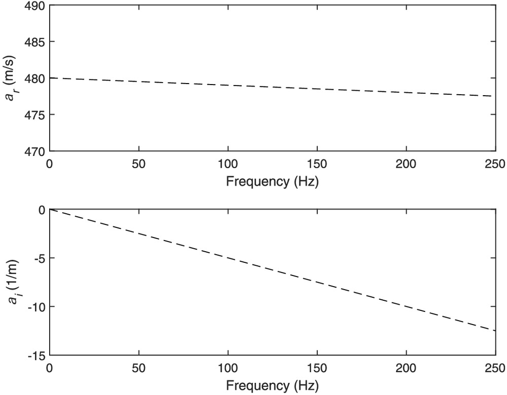
The frequency-dependent wave speed () and attenuation () relate to the complex wave speed through Eqs. (8) and (9)where the complex wave speed is described by , with and being the real and imaginary parts of the complex wave speed, respectively.
(8)
(9)
As can be seen from Eqs. (3) and (4), the complex wave speed and the complex wave number are connected by Eq. (10)
(10)
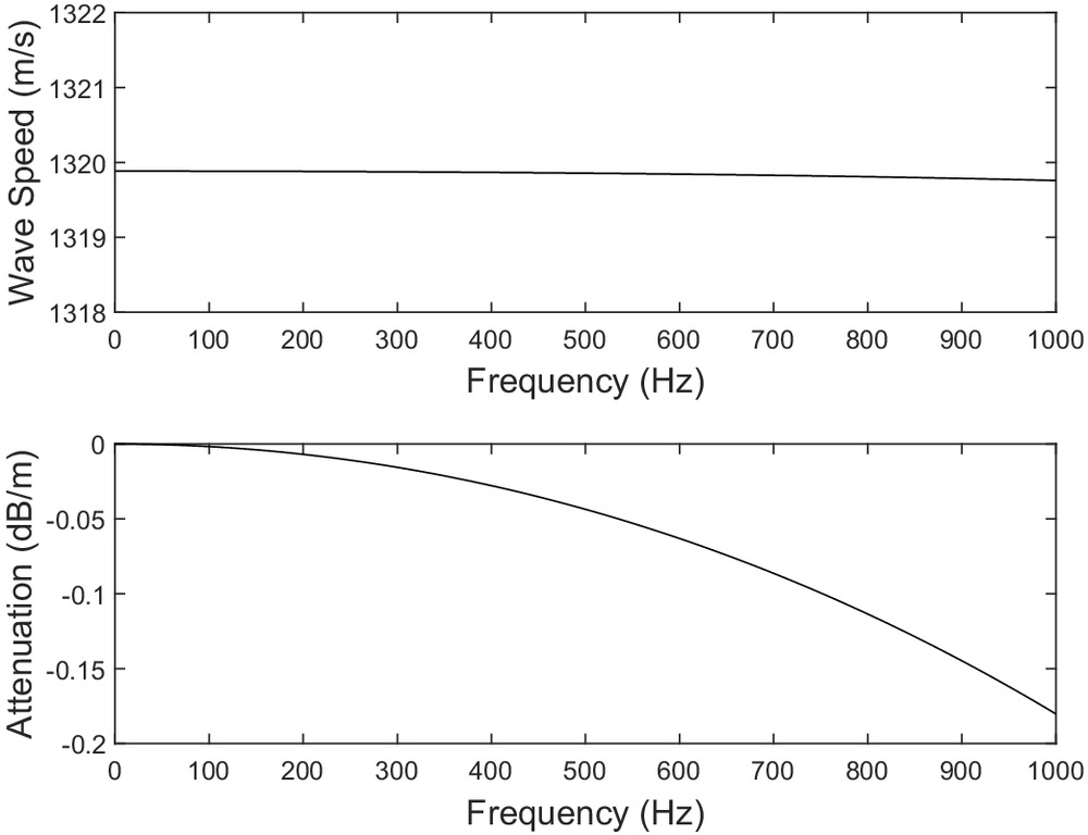
A complex wave speed , as shown in Fig. 3, has been assigned to the transfer matrix to simulate pressure response from the system in Fig. 2.
Excitations to the pipe system are simulated by oscillating the opening of the end valve (G), which is a common practice for transient simulations using the transfer matrix method (Gong et al. 2014). In this study, the dimensionless valve opening (normalized by the cross-sectional area of the pipe) oscillates around the mean opening area (the opening that results in the steady-state condition) following a random pattern with a rising/fall time of 0.01 s. The random pattern follows a standard normal distribution with a mean of zero and a variance of 0.01. The input to the transfer matrix model is the valve opening trace after converting it into the frequency domain.
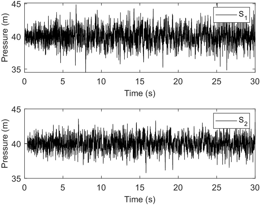
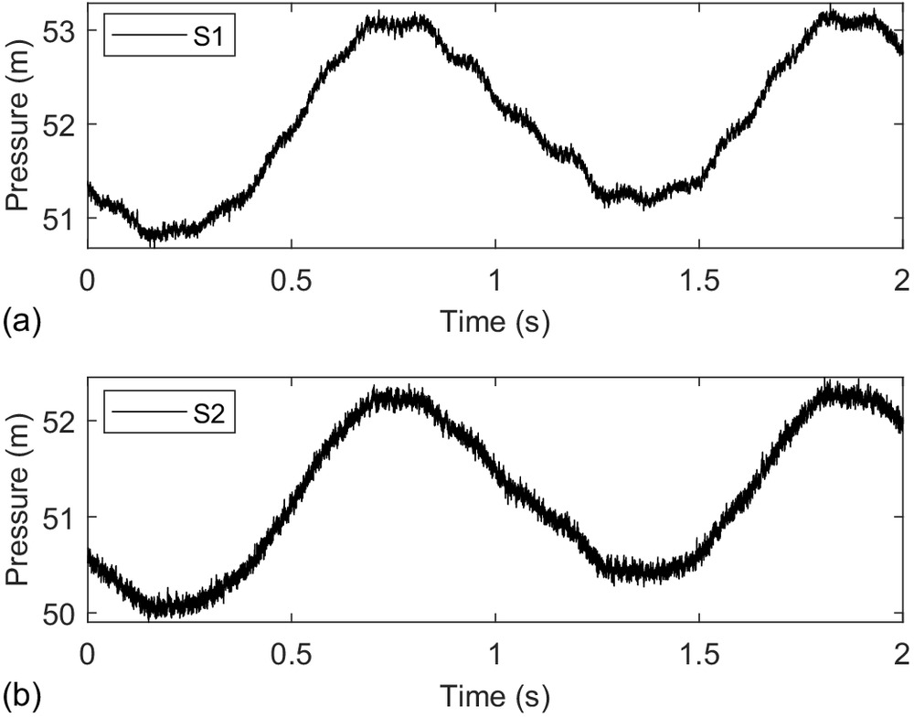
The frequency responses at two sensors ( and ) to the exciting valve are calculated by solving the equations formed by the transfer matrix method. Response to each frequency component is calculated within the frequency range of 0–4,000 Hz with a resolution of 0.05 Hz. To obtain the hydraulic pressure waves in the time domain, the frequency responses are converted to the time domain by the inverse Fourier transform (Suo and Wylie 1989). The pressure traces at and are shown in Fig. 4.
From the pressure responses at the two sensors ( and ), the paired-IRF can be determined by a deconvolution process, such as least-squares deconvolution (Nguyen et al. 2018). The result is shown in Fig. 5. The first positive spike is the time-domain representation of the transfer function for the pipe section between the two sensors.
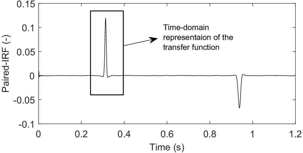
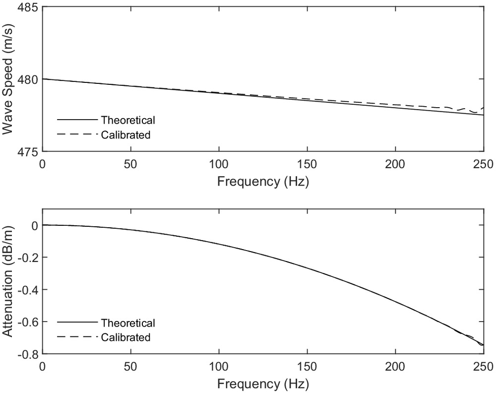
Fig. 6 shows the result of the calibrated frequency-dependent wave speed and attenuation rate using the paired-IRF trace. The calibrated wave speed and attenuation match well with the theoretical values used in the hydraulic model (as defined by the complex wave speed in Fig. 3), which validates the proposed technique. In the numerical model, the valve oscillations had a rising/fall time of 0.01 s. This limited the bandwidth of the generated pressure waves, and explains the small but increasing discrepancy between the “calibrated” and “theoretical” in the wave speed toward higher frequencies.
Experimental Validation
An HDPE pipe system and a copper pipe system were established in the hydraulics laboratory at the University of Adelaide. Three case studies were conducted, corresponding to three configurations. For the HDPE pipe, experiments were conducted for both the unburied and the buried configurations (Case 1 and Case 2). The copper pipe was anchored throughout at an interval of 0.5 m and the whole pipe was in the air (Case 3).
System Configuration
HDPE Pipe System (Case 1 and Case 2)
The schematic of the single HDPE pipe system is shown in Fig. 7. The upstream boundary of the pipe was connected to the water main. A valve was located at the downstream end of the pipe system. The end valve was closed during the test to pressurize the system. The internal diameter of the plastic pipe was 33.8 mm, and wall thickness was 3.2 mm. The HDPE pipe was anchored throughout at an interval of 2 m. Part of the HDPE pipe (2.5 m) was in a sand tray.
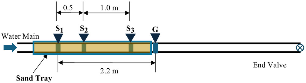
Persistent hydraulic waves were generated by a partially open side-discharge valve at point G in Fig. 7. Pressure responses were measured by three sensors (, and ) along the pipe. For the paired-IRF analysis, three pairs of sensors were formed (, , and ) and used as a cross-reference for each other pair. Distances for each pair of sensors were 0.5 m, 1.0 m, and 1.5 m for , , and , respectively. To assess uncertainty of the proposed method, three cases with varying distances are undertaken (0.5, 1.0, 1.5 m). Because these three cases are tested on the same pipe, consistent results are anticipated, thereby providing the uncertainty associated with the method. The sampling rate of the experiments was 50 kHz.
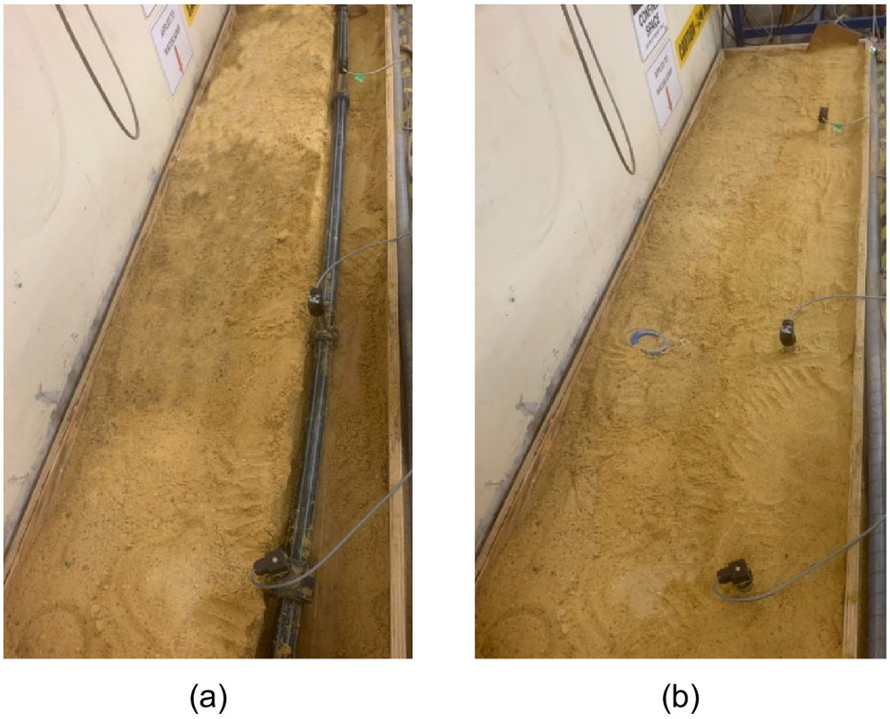
A sand tray was installed beneath the section of the pipe with three sensors for demonstrating the effect of surrounding soils (Fig. 8). Two cases were conducted with different soil conditions. As shown in Fig. 8, Case 1 was tested with the pipe in the air (laying on top of the soil), and in Case 2, the pipe section was buried in compacted shallow sand (about 10 cm).
Copper Pipe System (Case 3)
Experimental studies were also conducted on a copper pipe in the hydraulic laboratory at the University of Adelaide. Typically, the wave speed in an elastic pipe is assumed constant and the dispersion is negligible.
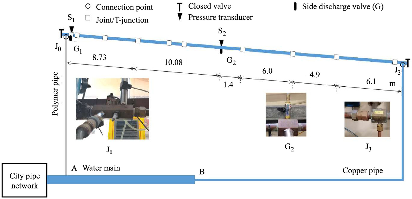
The schematic of the copper pipe system is shown in Fig. 9. The total length of the main pipe section J0–J3 was 37.46 m with an internal diameter of 22 mm. The two ends of the section of interest () were connected to the water main through a polymer pipe (garden hose) () and another copper pipe (), respectively. The pipe system was pressurized by the connected municipal water distribution system (WDS) and background pressure fluctuations and noise from the WDS propagated into the pipe system. Persistent hydraulic waves were generated as a form of persistent noise by a partially open side-discharge valve at point . By adjusting the opening of the valve, the magnitude and the frequency content of the persistent hydraulic waves could be adjusted. The pressure responses were measured by two sensors (, and ) along the pipe. The distance between the two sensors ( and ) was 18.81 m. The theoretical elastic wave speed of the pressure wave in the copper pipe is (Gong et al. 2018; Zeng et al. 2020a, b). The sampling rate of the experiments was 10 kHz.
Experimental Results
Case 1—HDPE Pipe in the Air
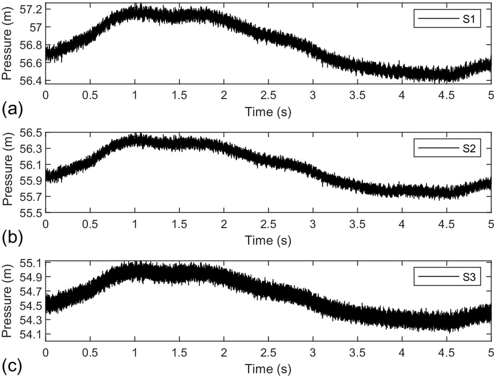
The first step of calibration is the determination of the paired-IRF using the pressure measurement at two sensors. As shown in Fig. 10, the magnitude of the persistent pressure responses measured at , , and was approximately 0.2 m.
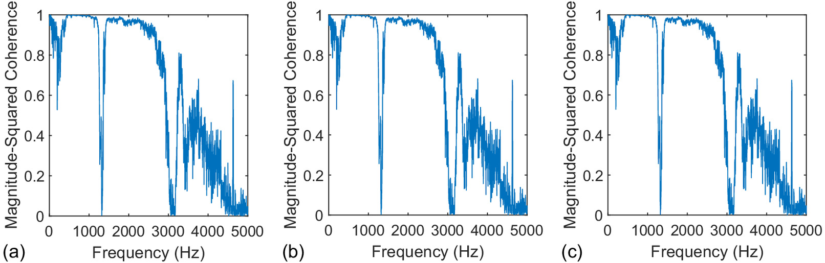
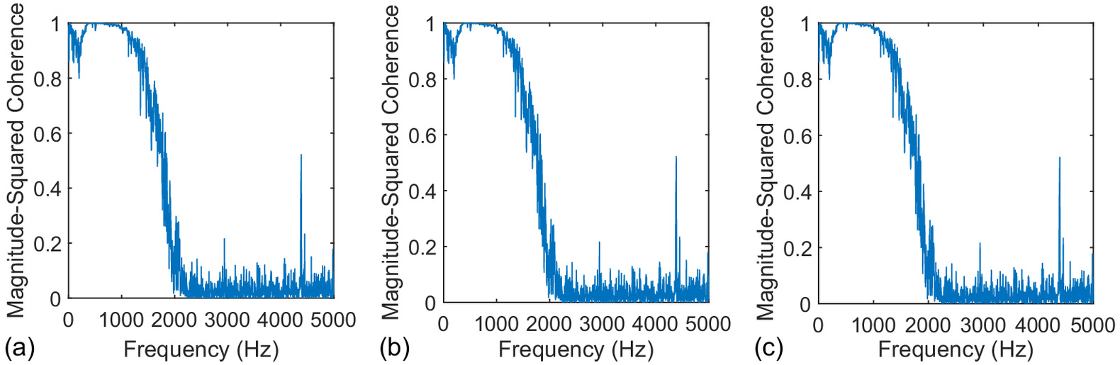
To find the frequency range in which strong causality exist between two signals, the magnitude-squared coherence was calculated for each pair of sensors. To enhance the robustness of calculation, the Hanning window was applied with a size of data points and 50% overlapping for each adjacent window.
For Case 1, the magnitude of coherence was close to 1 up to 2,500 Hz for all three pairs of sensors (except for low values around 1,300 Hz), and it gradually decreased from 2,500 to 3,000 Hz as shown in Fig. 11. The observed low coherence around 1,300 Hz might be attributed to interference or local resonance within the system, but the exact cause is unknown. Nevertheless, the low coherence was confined to a narrow band around 1,300 Hz, and the frequency range of interest was only up to 1,000 Hz. To remove the impact of interference in the frequencies higher than the range of interest, a lowpass filter was applied in MATLAB using the “lowpass” function (MathWorks 2022). The passband was set as 1,000 Hz and other control parameters were the default values (passband ripple 0.1 dB, transition band steepness 0.85, filter stopband attenuation 0.60 dB, and finite impulse response filter).
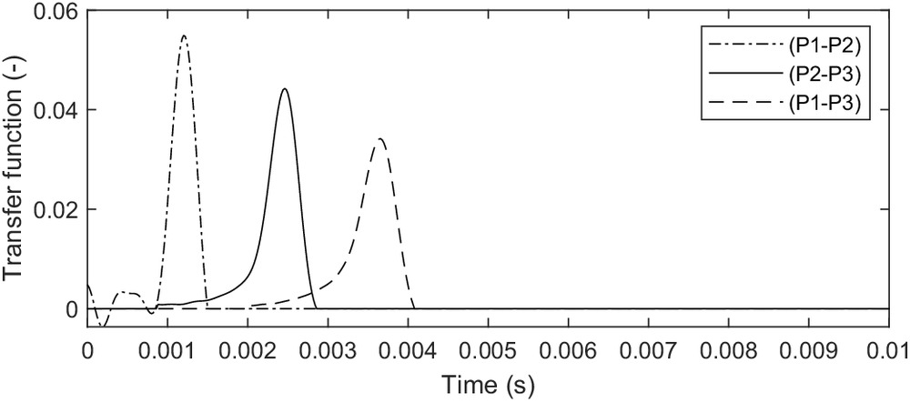
The paired-IRF were determined for each pair of sensors (, , and ). A record length of 60 s pressure data was used to determine each paired-IRF. To enhance the accuracy, the sliding window method was applied to the data. Each window had data points (corresponding to 5 s of data) and there was a 50% overlapping between two consecutive windows. Results from all the windows were averaged to yield the pared-IRF trace. As described in the methodology, the time-domain representation of the transfer function for the pipe section between each pair of sensors is represented by the first spike of the paired-IRF trace. Thus, the first spike was selected from each of the paired-IRF traces, as shown in Fig. 12.
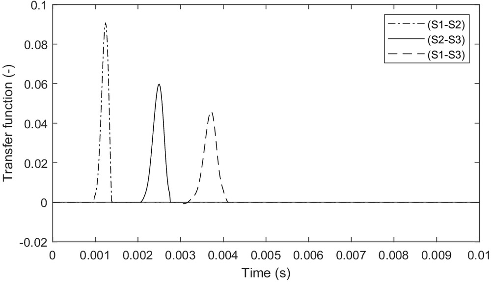
For Case 1, the magnitude of the first spike is 0.0956, 0.0597, and 0.0483 for sensor pair , , and , respectively. The occurrence time of the first peak for each pair is 0.00124, 0.00250, and 0.00372 s for , , and , respectively.
The calibrated frequency-dependent wave speed and attenuation were calculated as presented in Fig. 13 for three different sensor pairs. Note that the calculated frequency-dependent attenuation curves were all shifted to at 0 Hz. In the Fourier transform, the frequency zero component represents the average value of the signal. The transfer function is determined from the time-domain impulse response (Fig. 12) through Fourier transform. The impulse response used has a nonzero mean value, and the value is dependent on the distance between the two sensors. As a result, carries a nonzero value at 0 Hz, and that propagates to the attenuation rate at 0 Hz through Eqs. (4)–(7). Physically, frequency zero component refers to a constant signal, thus not dynamic waves. As a result, the original nonzero value of the attenuation rate at 0 Hz is a numerical artifact and should be offset.
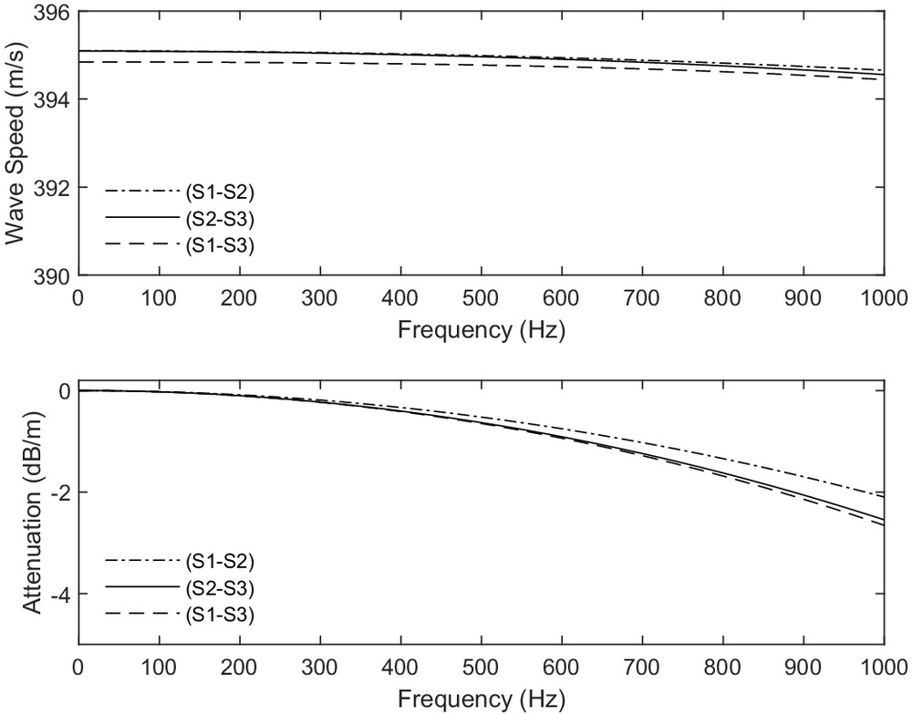
The frequency-dependent wave speed was at close to 0 Hz, and it gradually decreased with the increase in frequency but overall stable within the frequency range. The numerical value of the attenuation results also decreased with the increase in frequency, reaching about at 1,000 Hz. It should be noted that this means the attenuation rate increased with frequency (the negative sign means “loss” and the absolute value is the “rate”). The results from the three different sensor pairs show a high consistency for both the wave speed and attenuation, which validates the proposed calibration technique.
Case 2—HDPE Pipe Buried in Sand
To investigate the effect of the surrounding soils, the plastic pipe section of interest was buried in sand as shown in Fig. 8(b). The same procedure in Case 1 was followed to calibrate the frequency-dependent wave speed and attenuation, and the details are not repeated in this section.
To ensure the accuracy in results, a lowpass filter was selected based on the magnitude-squared coherence (Fig. 14). For Case 2, the magnitude of coherence was close to 1 up to 1,000 Hz for the three pairs of sensors. From 1,000 Hz, the coherence was gradually decreasing. Compared to Case 1 where the pipe was in air, the drop in coherence started from a much lower frequency, although the pressure excitation at the generator location would be similar. This indicates that, at the sensor location, the signal-to-noise ratio was lower in Case 2 than in Case 1, which was a result of higher attenuation caused by the surrounding sand. Nevertheless, because 0–1,000 Hz was the frequency range of focus and the coherence within this range was high, the same lowpass filter as used in Case 1 was applied to Case 2.
The time-domain representations of the transfer function were extracted as shown in Fig. 15. For Case 2, the magnitude of the transfer function is 0.0549, 0.0443, and 0.0341 for sensor pair , , and , respectively. The values are lower than the counterparts in Case 1, which again implies that higher attenuation effects were experienced when the pipe was buried in sand. Also, the width of the waveform in Case 2 (Fig. 15) is wider than that of Case 1 (Fig. 12), which indicates higher dispersion (wider distribution of the wave speed across frequencies).
The calibrated frequency-dependent wave speed and attenuation are presented in Fig. 16 for the three pairs of sensors. The results from pairs and show a high consistency for both wave speed and attenuation; however, the results from demonstrate some slight inconsistency from other results. As can be seen in Fig. 15, some fluctuations exist before 0.0008 s in the time-domain representation of the transfer function for the sensor pair . It implies that the attenuation and wave speed calibration is affected by noise observed in the paired-IRF trace.
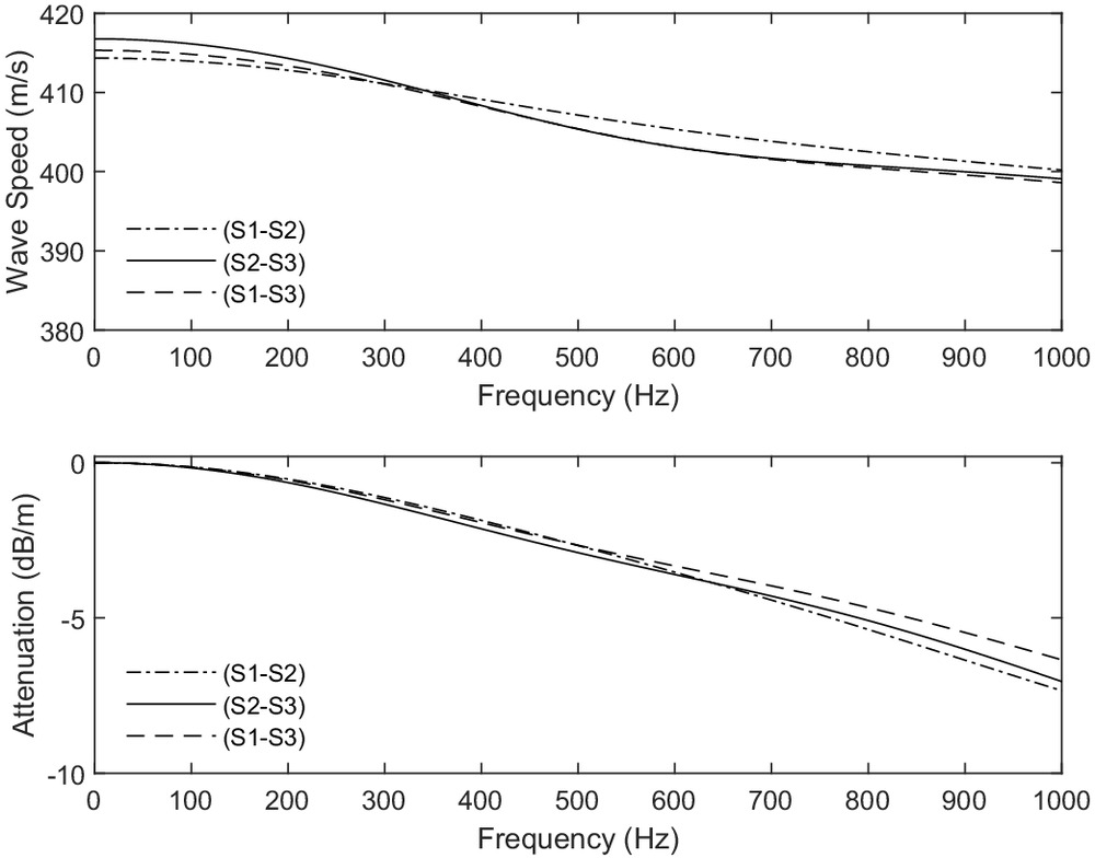
For Case 2, the frequency-dependent wave speed was at close to 0 Hz and decreased to at 1,000 Hz. The frequency-dependent attenuation was at 0 Hz and decreased to about /m at 1,000 Hz.
Compared to the results from Case 1 (pipe in the air), the wave speed is higher in Case 2 for the frequency range considered. Although they both show a decreasing trend, the gradient is larger in Case 2. Also, a much larger wave damping effect can be found in Case 2 based on the absolute value of the attenuation rate ( in Case 2 versus in Case 1 at 1,000 Hz).
The findings of case studies 1 and 2 show good agreement with the studies by Prek (2007) and Gao et al. (2017). Prek (2007) calibrated a PE pipe using a three-microphone method, resulting in a wave speed from about 366 to and an attenuation factor from approximately 0 to for the frequency range of 0–1,000 Hz. In Gao et al. (2017), the attenuation was gradually decreasing from approximately 0 to for frequency range of 0–800 Hz in an MDPE pipe. As discussed in Gao et al. (2017), the presence of soil as a surrounding medium contributes added stiffness and radiation damping to the pipe wall when compared to air as the surrounding material. Consequently, increase wave speed and greater attenuation are expected in pipes surrounded by soil compared to those in air.
Overall, the obvious difference in results between Cases 1 and 2 confirms that the proposed technique is sensitive and can detect the effect of surrounding materials. Like any experimental studies, there were uncertainties. In each case, three sets of results were obtained and the differences among them provide an indication of the extent of the uncertainty (because they should all reflect the same wave speed and attenuation). The uncertainties reflected by the two cases are similar, which is as expected. The extent of uncertainty is much smaller than the difference in the wave speed and attenuation rate between the two cases. Together with the fact that the results of Cases 1 and 2 were obtained from the same system with the only difference being the surrounding material, there is high confidence that the observed difference in wave speed and attenuation rate between the two cases is resulted from the impact of the sounding material.
Case 3—Copper Pipe
The copper pipe as shown in Fig. 9 was used in Case 3. The pressure traces measured at S1 and S2 are shown in Fig. 17. The magnitude of coherence is shown in Fig. 18. The coherence values were high (close to 1) up to 1,000 Hz for the pairs of sensors.
Based on the coherence, the same lowpass filter as used before was applied. The same procedure was followed to calibrate the frequency-dependent wave speed and attenuation. The extracted paired-IRF is shown in Fig. 19.
Using the first peak in the paired-IRF trace, the frequency-dependent wave speed and the attenuation coefficients were calculated as shown in Fig. 20. The wave speeds were very close to across the frequency range. The attenuation rates ranged from 0 to for 0–1,000 Hz.
Compared with the frequency-dependent wave characteristics in plastic pipes, the wave speed is much higher and the attenuation is significantly lower in the copper pipe. This is as expected and consistent with results in the literature.
Conclusion
In this paper, a new technique has been developed to calibrate the frequency-dependent wave speed and attenuation coefficient for pressure waves propagating in water pipes. A key innovation of the new technique is that it can conduct the calibration for a targeted pipe section as bracketed by two pressure sensors. This is achieved by analyzing the paired-IRF function determined from pressure responses measured by a pair of sensors. Using the first spike in the paired-IRF trace, the transfer function of the pipe section between the two sensors can be determined. Then, the frequency-dependent wave speed and attenuation are obtained from the real and imaginary part of the transfer function, respectively.
Numerical simulations have been conducted on a reservoir–pipeline–valve system to validate the proposed calibration technique. A complex wave speed was assigned to describe the pipe viscoelasticity, and the transfer matrix method was used to simulate the pressure responses. The calibrated frequency-dependent wave speed and attenuation using the proposed calibration method matched well with the original values assigned to the numerical model.
The frequency-dependent wave speed and attenuation of an HDPE pipe and a copper pipe have been calibrated using the proposed technique. The results showed that the HDPE pipe buried in sand experienced higher wave speeds and higher damping effects when compared to the same pipe section exposed to the air. The experimental results on the copper pipe demonstrated that the wave speeds were much higher and the attenuation rates were much smaller when compared to the HDPE pipe.
In real water pipelines, pressure measurements can be taken from existing access points such as air valves and fire hydrants (Gong et al. 2015, 2016a), which are typically tens of meters to a few hundred meters apart. This will enable the assessment of the frequency-dependent wave speed and attenuation for the pipe section between the selected two measurement locations, without excavation or suspending the service. If the pipe condition along the section is not uniform and wave reflections occur within the section, the frequency-dependent wave speed and attenuation can still be determined but they will carry higher uncertainties. The results represent the average condition of the pipe section. For pipelines with very limited access, in-pipe pressure sensor arrays can be used (Gong et al. 2018), which can also improve the spatial resolution.
The developed new technique can be used for discerning diverse wave propagation characteristics related to pipe material or mechanical properties, which is useful for the calibration of hydraulic models. The technique also has the potential to serve as a nondestructive pipe condition assessment tool, because it is expected that deterioration in pipe wall material or mechanical conditions would result in changes in the frequency-dependent wave speed and attenuation. This will be particularly useful to plastic pipe and asbestos cement pipes, where the material deterioration is difficult to detect by visual inspections (e.g., traditional CCTV inspections). However, in addition to pipe deterioration, many factors contribute to the frequency-dependent wave speed and attenuation (e.g., pipe material, soil condition, temperature, etc.). Future research should investigate the impact to the frequency-dependent wave speed and attenuation from individual factors.
Data Availability Statement
Some of the experimental data and numerical code that support the findings of this study are available from the corresponding author upon reasonable request.
Acknowledgments
The research presented in the paper has been supported by the Australian Research Council through the Linkage Project scheme (LP180100569).
References
Abdel-Gawad, H. A., and B. Djebedjian. 2020. “Modeling water hammer in viscoelastic pipes using the wave characteristic method.” Appl. Math. Modell. 83 (Jul): 322–341. https://doi.org/10.1016/j.apm.2020.01.045.
Ayati, A. H., and A. Haghighi. 2023. “Multiobjective wrapper sampling design for leak detection of pipe networks based on machine learning and transient methods.” J. Water Resour. Plann. Manage. 149 (2): 04022076. https://doi.org/10.1061/JWRMD5.WRENG-5620.
Bergant, A., A. S. Tijsseling, J. P. Vítkovský, D. I. Covas, A. R. Simpson, and M. F. Lambert. 2008. “Parameters affecting water-hammer wave attenuation, shape and timing—Part 2: Case studies.” J. Hydraul. Res. 46 (3): 382–391. https://doi.org/10.3826/jhr.2008.2847.
Brennan, M. J., Y. Gao, and P. F. Joseph. 2007. “On the relationship between time and frequency domain methods in time delay estimation for leak detection in water distribution pipes.” J. Sound Vib. 304 (1–2): 213–223. https://doi.org/10.1016/j.jsv.2007.02.023.
Brunone, B. 1999. “Transient test-based technique for leak detection in outfall pipes.” J. Water Resour. Plann. Manage. 125 (5): 302–306. https://doi.org/10.1061/(ASCE)0733-9496(1999)125:5(302).
Chaudhry, M. H. 2014. Applied hydraulic transients. 3rd ed. New York: Springer.
Che, T.-C., H.-F. Duan, and P. J. Lee. 2021. “Transient wave-based methods for anomaly detection in fluid pipes: A review.” Mech. Syst. Signal Process. 160 (Nov): 107874. https://doi.org/10.1016/j.ymssp.2021.107874.
Covas, D., and H. Ramos. 2010. “Case studies of leak detection and location in water pipe systems by inverse transient analysis.” J. Water Resour. Plann. Manage. 136 (2): 248–257. https://doi.org/10.1061/(ASCE)0733-9496(2010)136:2(248).
Covas, D., I. Stoianov, J. F. Mano, H. Ramos, N. Graham, and C. Maksimovic. 2005. “The dynamic effect of pipe-wall viscoelasticity in hydraulic transients. Part II—Model development, calibration and verification.” J. Hydraul. Res. 43 (1): 56–70. https://doi.org/10.1080/00221680509500111.
Covas, D., I. Stoianov, H. Ramos, N. Graham, and C. Maksimovic. 2004. “The dynamic effect of pipe-wall viscoelasticity in hydraulic transients. Part I—Experimental analysis and creep characterization.” J. Hydraul. Res. 42 (5): 516–530. https://doi.org/10.1080/00221686.2004.9641221.
Duan, H. 2016. “Sensitivity analysis of a transient-based frequency domain method for extended blockage detection in water pipeline systems.” J. Water Resour. Plann. Manage. 142 (4): 04015073. https://doi.org/10.1061/(ASCE)WR.1943-5452.0000625.
Duan, H.-F., M. Ghidaoui, P. J. Lee, and Y.-K. Tung. 2010. “Unsteady friction and visco-elasticity in pipe fluid transients.” J. Hydraul. Res. 48 (3): 354–362. https://doi.org/10.1080/00221681003726247.
Evangelista, S., A. Leopardi, R. Pignatelli, and G. de Marinis. 2015. “Hydraulic transients in viscoelastic branched pipelines.” J. Hydraul. Eng. 141 (8): 04015016. https://doi.org/10.1061/(ASCE)HY.1943-7900.0001030.
Fox, G., Jr., and D. Stepnewski. 1974. “Pressure wave transmission in a fluid contained in a plastically deforming pipe.” J. Pressure Vessel Technol. 96 (4): 258–262. https://doi.org/10.1115/1.3454178.
Gally, M., M. Guney, and E. Rieutord. 1979. “An investigation of pressure transients in viscoelastic pipes.” J. Fluids Eng. 101 (4): 495–499. https://doi.org/10.1115/1.3449017.
Gao, Y., M. Brennan, P. F. Joseph, J. M. Muggleton, and O. Hunaidi. 2005. “On the selection of acoustic/vibration sensors for leak detection in plastic water pipes.” J. Sound Vib. 283 (3–5): 927–941. https://doi.org/10.1016/j.jsv.2004.05.004.
Gao, Y., Y. Liu, and J. M. Muggleton. 2017. “Axisymmetric fluid-dominated wave in fluid-filled plastic pipes: Loading effects of surrounding elastic medium.” Appl. Acoust. 116 (Jan): 43–49. https://doi.org/10.1016/j.apacoust.2016.09.016.
Gong, J., M. Lambert, A. Zecchin, A. Simpson, N. Arbon, and Y.-I. Kim. 2016a. “Field study on non-invasive and non-destructive condition assessment for asbestos cement pipelines by time-domain fluid transient analysis.” Struct. Health Monit. 15 (1): 113–124. https://doi.org/10.1177/1475921715624505.
Gong, J., G. M. Png, J. W. Arkwright, A. W. Papageorgiou, P. R. Cook, M. F. Lambert, A. R. Simpson, and A. C. Zecchin. 2018. “In-pipe fibre optic pressure sensor array for hydraulic transient measurement with application to leak detection.” Measurement 126 (Oct): 309–317. https://doi.org/10.1016/j.measurement.2018.05.072.
Gong, J., M. L. Stephens, N. S. Arbon, A. C. Zecchin, M. F. Lambert, and A. R. Simpson. 2015. “On-site non-invasive condition assessment for cement mortar–lined metallic pipelines by time-domain fluid transient analysis.” Struct. Health Monit. 14 (5): 426–438. https://doi.org/10.1177/1475921715591875.
Gong, J., A. C. Zecchin, M. F. Lambert, and A. R. Simpson. 2016b. “Determination of the creep function of viscoelastic pipelines using system resonant frequencies with hydraulic transient analysis.” J. Hydraul. Eng. 142 (9): 04016023. https://doi.org/10.1061/(ASCE)HY.1943-7900.0001149.
Gong, J., A. C. Zecchin, A. R. Simpson, and M. F. Lambert. 2014. “Frequency response diagram for pipeline leak detection: Comparing the odd and even harmonics.” J. Water Resour. Plann. Manage. 140 (1): 65–74. https://doi.org/10.1061/(ASCE)WR.1943-5452.0000298.
Hunaidi, O., and W. T. Chu. 1999. “Acoustical characteristics of leak signals in plastic water distribution pipes.” Appl. Acoust. 58 (3): 235–254. https://doi.org/10.1016/S0003-682X(99)00013-4.
Landry, C., C. Nicolet, A. Bergant, A. Müller, and F. Avellan. 2012. “Modeling of unsteady friction and viscoelastic damping in piping systems.” IOP Conf. Ser.: Earth Environ. Sci. 15 (5): 052030. https://doi.org/10.1088/1755-1315/15/5/052030.
MathWorks. 2022. MATLAB version: 9.12.0 (R2022a). Natick, MA: MathWorks Inc.
Meniconi, S., B. Brunone, M. Ferrante, and C. Massari. 2012. “Transient hydrodynamics of in-line valves in viscoelastic pressurized pipes: Long-period analysis.” Exp. Fluids 53 (Jul): 265–275. https://doi.org/10.1007/s00348-012-1287-3.
Mitosek, M., and A. Roszkowski. 1998. “Empirical study of water hammer in plastics pipes.” Plast. Rubber Compos. Process. Appl. 27 (9): 436–439.
Muggleton, J. M., M. J. Brennan, and P. W. Linford. 2004. “Axisymmetric wave propagation in fluid-filled pipes: Wavenumber measurements in in vacuo and buried pipes.” J. Sound Vib. 270 (1–2): 171–190. https://doi.org/10.1016/S0022-460X(03)00489-9.
Muggleton, J. M., M. J. Brennan, and R. J. Pinnington. 2002. “Wavenumber prediction of waves in buried pipes for water leak detection.” J. Sound Vib. 249 (5): 939–954. https://doi.org/10.1006/jsvi.2001.3881.
Muggleton, J. M., and J. Yan. 2013. “Wavenumber prediction and measurement of axisymmetric waves in buried fluid-filled pipes: Inclusion of shear coupling at a lubricated pipe/soil interface.” J. Sound Vib. 332 (5): 1216–1230. https://doi.org/10.1016/j.jsv.2012.10.024.
Nguyen, S. T. N., J. Gong, M. F. Lambert, A. C. Zecchin, and A. R. Simpson. 2018. “Least squares deconvolution for leak detection with a pseudo random binary sequence excitation.” Mech. Syst. Signal Process. 99 (Jan): 846–858. https://doi.org/10.1016/j.ymssp.2017.07.003.
Pezzinga, G., B. Brunone, D. Cannizzaro, M. Ferrante, S. Meniconi, and A. Berni. 2014. “Two-dimensional features of viscoelastic models of pipe transients.” J. Hydraul. Eng. 140 (8): 04014036. https://doi.org/10.1061/(ASCE)HY.1943-7900.0000891.
Prek, M. 2007. “Analysis of wave propagation in fluid-filled viscoelastic pipes.” Mech. Syst. Signal Process. 21 (4): 1907–1916. https://doi.org/10.1016/j.ymssp.2006.07.013.
Soares, A. K., D. I. Covas, and L. F. Reis. 2008. “Analysis of PVC pipe-wall viscoelasticity during water hammer.” J. Hydraul. Eng. 134 (9): 1389–1394. https://doi.org/10.1061/(ASCE)0733-9429(2008)134:9(1389).
Stephens, M., J. Gong, C. Zhang, A. Marchi, L. Dix, and M. F. Lambert. 2020. “Leak-before-break main failure prevention for water distribution pipes using acoustic smart water technologies: Case study in Adelaide.” J. Water Resour. Plann. Manage. 146 (10): 05020020. https://doi.org/10.1061/(ASCE)WR.1943-5452.0001266.
Stephens, M. L., M. F. Lambert, A. R. Simpson, and J. P. Vitkovsky. 2011. “Calibrating the water-hammer response of a field pipe network by using a mechanical damping model.” J. Hydraul. Eng. 137 (10): 1225–1237. https://doi.org/10.1061/(ASCE)HY.1943-7900.0000413.
Suo, L., and E. B. Wylie. 1989. “Impulse response method for frequency-dependent pipeline transients.” J. Fluids Eng. 111 (4): 478–483. https://doi.org/10.1115/1.3243671.
Suo, L., and E. B. Wylie. 1990. “Complex wavespeed and hydraulic transients in viscoelastic pipes.” J. Fluids Eng. 112 (4): 496–500. https://doi.org/10.1115/1.2909434.
Tijsseling, A. S., M. F. Lambert, A. R. Simpson, M. L. Stephens, J. P. Vítkovský, and A. Bergant. 2006. “Wave front dispersion due to fluid-structure interaction in long liquid-filled pipelines.” In Proc., 23rd IAHR Symp. on Hydraulic Machinery and Systems. Madrid, Spain: International Association for Hydro-Environment Engineering and Research.
Wang, X., J. Lin, and M. S. Ghidaoui. 2020. “Usage and effect of multiple transient tests for pipeline leak detection.” J. Water Resour. Plann. Manage. 146 (11): 06020011. https://doi.org/10.1061/(ASCE)WR.1943-5452.0001284.
Wylie, E. B., and V. L. Streeter. 1993. Fluid transients in systems. Englewood Cliffs, NJ: Prentice Hall.
Zecchin, A. C., N. Do, J. Gong, M. Leonard, M. F. Lambert, and M. L. Stephens. 2022. “Optimal pipe network sensor layout design for hydraulic transient event detection and localization.” J. Water Resour. Plann. Manage. 148 (8): 04022041. https://doi.org/10.1061/(ASCE)WR.1943-5452.0001536.
Zeng, W., J. Gong, A. R. Simpson, B. S. Cazzolato, A. C. Zecchin, and M. F. Lambert. 2020a. “Paired-IRF method for detecting leaks in pipe networks.” J. Water Resour. Plann. Manage. 146 (5): 04020021. https://doi.org/10.1061/(ASCE)WR.1943-5452.0001193.
Zeng, W., J. Gong, A. C. Zecchin, M. F. Lambert, A. R. Simpson, and B. S. Cazzolato. 2018. “Condition assessment of water pipelines using a modified layer-peeling method.” J. Hydraul. Eng. 144 (12): 04018076. https://doi.org/10.1061/(ASCE)HY.1943-7900.0001547.
Zeng, W., A. C. Zecchin, J. Gong, M. F. Lambert, A. R. Simpson, and B. S. Cazzolato. 2020b. “Inverse wave reflectometry method for hydraulic transient-based pipeline condition assessment.” J. Hydraul. Eng. 146 (8): 04020056. https://doi.org/10.1061/(ASCE)HY.1943-7900.0001785.
Information & Authors
Information
Published In

Journal of Water Resources Planning and Management
Volume 150 • Issue 11 • November 2024
Copyright
This work is made available under the terms of the Creative Commons Attribution 4.0 International license, https://creativecommons.org/licenses/by/4.0/.
History
Received: Aug 29, 2023
Accepted: Jun 17, 2024
Published online: Aug 30, 2024
Published in print: Nov 1, 2024
Discussion open until: Jan 30, 2025
Authors
Metrics & Citations
Metrics
Citations
Download citation
If you have the appropriate software installed, you can download article citation data to the citation manager of your choice. Simply select your manager software from the list below and click Download.