Opportunities for Restoring Environmental Flows in the Rio Grande–Rio Bravo Basin Spanning the US–Mexico Border

Richter, Brian D.; Prunes, Enrique; Liu, Ning; Caldwell, Peter; Wei, Dongyang; Davis, Kyle Frankel; Sandoval-Solis, Samuel; Herrera, Gabriela Rendon; Rodriguez, Ramon Saiz; Ao, Yufei; Lamsal, Gambhir; Amaya, Maria; Shahbol, Natalie; Marston, Landon

doi:10.1061/JWRMD5.WRENG-6278

Open access

Technical Papers

Nov 22, 2023

Opportunities for Restoring Environmental Flows in the Rio Grande–Rio Bravo Basin Spanning the US–Mexico Border

Publication: Journal of Water Resources Planning and Management

Volume 150, Issue 2

https://doi.org/10.1061/JWRMD5.WRENG-6278

PDF

Abstract

The Rio Grande–Rio Bravo’s flow regime has been highly altered for more than 130 years, yet the river ecosystem still supports important biodiversity including numerous endangered species. More than 80% of water consumed in the basin goes to irrigating farms, but in recent decades, farmers have repeatedly experienced severe water shortages. Given this water-scarce condition, any plans for enhancing environmental flows must be carefully designed to minimize impacts or provide benefits to agriculture. This study describes the development of the Rio Grande–Rio Bravo’s first whole-basin hydrologic model—representing both the United States and Mexico portions of the basin—to enable exploration of environmental flow restoration needs and options for meeting these needs. We then demonstrate an analytical process in which environmental flow needs are compared to existing flow conditions to quantify gaps, and then evaluate how those gaps can be filled by reducing farm irrigation needs by shifting to less water-intensive crops and fallowing a portion of existing farmland while maintaining or improving net revenues. In our pilot assessment we find that an improvement of

{2.2 m}^{3} / s

would fill the environmental flow gap for late-summer low-flow conditions at Albuquerque, New Mexico. This flow enhancement is attainable by fallowing 18%–26% of cropland and shifting to more profitable and less water-intensive crops to sustain overall farm revenues.

Introduction

There are few river systems in the world that have experienced such massive transformation so rapidly: in just 50 years, from the 1880s to the 1930s, the Rio Grande–Rio Bravo (RGRB) was converted from a largely natural, free-flowing river into a heavily depleted and laterally constrained channel fully harnessed for farm irrigation (Vick 2012; Blythe and Schmidt 2018; Garza-Diaz and Sandoval-Solis 2022; Sandoval-Solis et al. 2022). That makeover has largely persisted throughout the last century.

However, the river continues to provide many important benefits in addition to irrigated agriculture, which accounts for 83% of all water consumed for human purposes in the basin (Sandoval-Solis et al. 2022). The river basin—half of which lies in Mexico, where it is known as the Rio Bravo—encompasses

{557,000 km}^{2}

(

{215,000 mi}^{2}

); the river flows more than 3,000 km (1,900 mi) from its Rocky Mountain headwaters to the Gulf of Mexico (Fig. 1). It irrigates more than

{7,800 km}^{2}

(

{3,012 mi}^{2}

) of farmland (Garza-Diaz and Sandoval-Solis 2022) and provides drinking water for 11 million people in Mexico (INEGI 2010) and 4 million within the United States (Plassin et al. 2020), including the major population centers of Albuquerque and El Paso in the United States and Chihuahua and Monterrey in Mexico.

Fig. 1. Rio Grande–Rio Bravo basin. [Sources: Esri, HERE, Garmin, Intermnap, increment P Corp., GEBCO, USGS, FAO, NPS, NRCAN, GeoBase, IGN, Kadaster NL, Ordinance Survey, Esri Japan, METI, Esri China (Hong Kong), © OpenStreetMap contributors, and the GIS User Community; Sources: Esri, USGS, NOAA; Data from USGS 2015, 2016, 2020; Plassin et al. 2020; CONABIO 2018.]

The basin is renowned for its biological diversity and endemism: nearly half of the basin’s native fish species are found nowhere else, and wetlands and riparian forests supported by the river are critically important to birds migrating along the Central Flyway (Pronatura Noreste 2004). The river flowed perennially throughout its length prior to 1880, but it is now seasonally dry or nearly so in multiple segments (Dean and Schmidt 2011; Blythe and Schmidt 2018); flow depletion is a major factor in the imperilment of at least 75 species supported by the river system (Richter et al. 2016) (Table S1). Conservation interests are now envisioning the remaining discontinuous but perennially flowing habitats along the river corridor as a “string of ecological pearls” needing environmental flow restoration (Sandoval-Solis et al. 2022).

To explore the potential for restoring some semblance of the historical flow regime characteristics along the RGRB, we followed four sequential steps:

1.

After extensive review of hydrologic modeling to date (Ortiz-Partida et al. 2017), we developed what we believe to be the first hydrologic simulation model encompassing the entirety of the RGRB basin, to be used in assessing flow depletion and restoration options throughout the basin.

2.

We utilized the hydrologic model as a screening tool to assess the volume of potential irrigation savings in each subbasin that could be used in restoring environmental flows.

3.

We compared these potential restoration volumes with “environmental flow gaps” for various river locations (Patterson and Sandoval-Solis 2022).

4.

We assessed crop-shifting and fallowing strategies (Richter et al. 2022) as opportunities for achieving the reductions in irrigation needed to fill critical environmental flow gaps.

Before describing our methods and results in greater detail, we summarize here the sequence of water development projects that created the highly altered state of today’s river.

Water Infrastructure and Policy Development

The RGRB’s flow was increasingly depleted over five general phases of infrastructure development. The operation of this infrastructure is strongly controlled by intrastate, interstate, and international policies.

Headwaters Irrigation Phase

Major depletions of the river’s natural flow began with settlement of the San Luis Valley, in the RGRB headwaters in Colorado (Fig. 1). Discoveries of gold in California, the promise of free farmland from the federal Homestead Act of 1862 and the Desert Land Act of 1877, expansion of rail lines across the Western United States, and passage of the Indian Appropriations Act of 1871—which forcefully moved native tribes onto reservations—stimulated a massive westward migration of hundreds of thousands of settlers from the eastern United States in the late 1800s (Vick 2012).

Large irrigation canals were constructed in San Luis Valley in the 1880s to irrigate nearly 121,000 hectares (300,000 acres) of new farmland and produce food for a growing population (Montgomery Watson Harza 2001). River irrigation was supplemented with an estimated 2,000 groundwater wells by 1891 (there are more than 10,000 today) (Stiller 2021). The valley farms also produced fodder for immense herds of livestock that were exported from the valley to distant markets by newly established rail lines. By 1890, there was very little Rio Grande water flowing south into New Mexico during the summer growing season, which is a condition that persists today (Horgan 1984; Blythe and Schmidt 2018; Stiller 2021).

International Water-Sharing Agreement and Large Reservoir Construction in the United States

The depletion of headwater flows in the San Luis Valley could be felt as far downstream as the Juarez Valley near Chihuahua, Mexico. Lacking water to irrigate fields that had been cultivated for centuries, the Mexican government lodged formal complaints with the United States beginning in 1894 (Vick 2012). In response, an international water-sharing agreement known as the Rio Grande Convention was negotiated and adopted in 1906 that guaranteed delivery of

74 \times 10^{6} m^{3}

of water (which is equal to

60,000 acre / ft

) to Mexico each year, or about 3% of the river’s flow at Juarez (Phillips et al. 2015). The Convention also allocated shares of water to the Mesilla Valley in New Mexico and the El Paso Valley in Texas.

The 1906 Convention was the first of three critically important water-sharing agreements that have sustained the river’s freshwater biodiversity by mandating that some portion of the river’s water would be pulled all the way downstream from Colorado into Texas, and from the Big Bend region into the river’s lowest reaches near the Gulf of Mexico. When negotiating the 1906 Convention, farming interests in the Mesilla and El Paso valleys promoted the idea that a new reservoir was needed to capture whatever snowmelt runoff escaped diversions in Colorado (Phillips et al. 2015). This reservoir storage would both ensure that Mexico’s water allocation for the Juarez Valley could be delivered and enable expanded irrigation farming in the Mesilla and El Paso valleys on the United States side of the river.

The resulting “Rio Grande Project” constructed hundreds of kilometers of irrigation canals and pipes, as well as extensive levees to constrict the river’s tendency to move around during floods (Autobee 1994). The project’s centerpiece was an enormous new reservoir named Elephant Butte, completed in 1916, capable of storing two full years of average river flow. The area of irrigated land in the Mesilla Valley tripled in extent (Phillips et al. 2015).

Emboldened with a more reliable water supply, the Mesilla Valley farmers ironically poured so much water onto their farms that they quickly became waterlogged, requiring installation of drainage systems (Phillips et al. 2015). Once the irrigation systems in the Mesilla Valley were tightened up, and the Juarez Valley on the Mexican side of the RGRB began to prosper with an assured water supply, the drying of the river downstream of El Paso, Texas, was virtually complete. Today, only occasional flushes of monsoon (summer) stormwater pass through the 240-km (150-mi) reach from Fort Quitman to Presidio known as the “Forgotten Reach” (Fig. 1).

Reservoir Development in Mexico

During the early 1900s, while the northern branch of the river above Fort Quitman was being heavily depleted from irrigation far upstream in the San Luis Valley, an infusion of water from the Rio Conchos—the largest tributary in Mexico—continued to revive the river as it entered a sequence of canyons along the US–Mexico border that eventually became part of Big Bend National Park in 1935. As the Americans were building the Rio Grande Project, the Mexico’s National Irrigation Commission was simultaneously investing in their own irrigation initiatives on the Rio Conchos. The massive La Boquilla Reservoir was completed in 1916, large enough to store two full years of Conchos flow. This new reservoir enabled creation of the expansive “Delicias” irrigation district, which along with two other smaller irrigation districts consumes half of the Conchos flow on average, leaving the remaining half to flow through the Big Bend segment of the RGRB (Phillips et al. 2015).

Interstate Water-Sharing Agreement

While the Rio Grande Project and the Rio Conchos irrigation systems were being constructed, another group of settlers in the area around Albuquerque began developing their own plans for irrigation improvements that included drainage of water-logged land, construction of levees, and a new El Vado Dam on the Rio Chama, a major tributary in New Mexico, to facilitate increased irrigation. These plans were enabled by the formation of the Middle Rio Grande Conservancy District in the mid-1920s.

The new irrigation district was also viewed as a threat to the viability of the downstream Rio Grande Project because the new district could intercept water that otherwise would have made its way to Elephant Butte Reservoir (Phillips et al. 2015). As El Vado Dam was being constructed, Texas sued New Mexico to stop the development. Similarly, fearing potential growth in water use in the San Luis Valley, New Mexico sought to restrain Colorado from further depleting the river. The resolution to these conflicts was the Rio Grande Compact, signed in 1938, that specified how much water Colorado must pass downstream to New Mexico, and reaffirmed that Texas would get the water it was allocated under the Rio Grande Project (Phillips et al. 2015; Vick 2012). In effect, a small portion of the river’s natural flow was thereby assured to cross multiple state lines, providing some sustenance to the river ecosystem along the way.

International Cooperation to Build Reservoirs and Share the Lower River

While the 1906 Convention and the 1938 Compact did manage to sustain a minimum annual flow of water through New Mexico and into west Texas, many of the river’s species and ecosystems were gravely imperiled by the end of the 1930s. No longer could shovelnose sturgeon (Scaphirhynchus platorynchus), Longnose gar (Lepisosteus osseus), Gizzard shad (Dorosoma cepedianum), or American eels (Anguilla rostrata) swim upstream from the Gulf of Mexico into northern New Mexico (Crawford et al. 1993; Phillips et al. 2015). Flow depletion and elimination of natural flooding pushed numerous native species to the brink of extinction (Richter et al. 2016).

Yet still, along the lowermost 2,000 km (1,250 mi) of the RGRB there were additional farmers longing for more water on both sides of the international border. The two countries realized that it would be in their mutual interest to formalize each country’s entitlement to the lower river and its tributaries, resulting in the Treaty for the Utilization of the Waters of the Colorado and Tijuana Rivers and of the Rio Grande (known as the “1944 Water Treaty”; Enriquez-Coyro 1976; Phillips et al. 2015). For the RGRB, the Treaty allocates to Mexico: (1) all of water from the San Juan and Alamo Rivers; (2) two-thirds of the flow of six other Mexican tributaries, including the Rio Conchos; and (3) one-half of all other flows occurring in the main channel of the RGRB downstream from Fort Quitman. The two-thirds from the six Mexican tributaries shall not be less than

432.3 \times 10^{6} m^{3}

per year (

350,000 acre / ft / year

) on average over a treaty cycle of five consecutive years. The Treaty allocates to the United States: (1) water from six tributaries and one spring on the US side, (2) one-third of the water from six Mexican tributaries including the Rio Conchos, and (3) one-half of all other flows occurring in the main channel of the RGRB downstream from Fort Quitman.

To enable optimal use of the water flowing into and through the lower river, the two countries collaborated in building two more big reservoirs—Falcon Reservoir in 1953 and Amistad Reservoir in 1969—to capture what remained of the river for irrigation use in the lower river basin (Fig. 1). Today, the only water flowing out the mouth of the river is what drains off farm fields adjacent to the river’s lowermost reaches.

Effects of Water-Sharing Agreements on Flow Regime

The three water-sharing agreements (1906 Convention, 1938 Compact, and 1944 Treaty) have been essential to ensuring that some water continues to flow from Colorado to Texas and Mexico. While the purpose of these legal agreements is to facilitate water sharing among the states and countries, they also ensure that water moves through the river ecosystem.

Fig. 2 illustrates the volumes of water that have been conveyed through the river system since 2000 as a direct result of these water-sharing agreements. The pattern (timing and volume) of water deliveries throughout the year is carefully managed using irrigation curtailments and reservoir releases, primarily for the purpose of providing irrigation water when it is needed and minimizing conveyance losses (Vandiver 1999; Nava and Sandoval-Solis 2014). However, as Fig. 3 and Table S2 reveal, the river’s flow remains severely depleted throughout the river system.

Fig. 2. Annual deliveries under water-sharing agreements. The volume of annual water deliveries associated with the 1938 Compact (CO to NM deliveries and NM to TX deliveries) and the 1944 Treaty (Mexico to US deliveries, including contributions from the Rio Conchos and five other Mexican tributaries). Note that 100 million cubic meters equals $\sim 2,300 acre / ft$ .

Fig. 3. Depletion of RGRB flow regime. Daily averages and range of flows for both natural (blue line and shading) and observed conditions (red line and shading) are shown here for four locations along the RGRB, based on the period of 1975–2020. Lines indicate daily medians, shading indicates interquartile range of daily observations or estimates: (a) the Lobatos gauge is representative of flows from Colorado into New Mexico (RGRB near Lobatos, CO); (b) the El Paso gauge in Texas is representative of flows from New Mexico into Texas (RGRB El Paso, TX); (c) the Johnson Ranch gauge is representative of flows in the Big Bend reach downstream of the confluence with the Rio Conchos inflow from Mexico (RGRB Johnson Ranch, TX); and (d) the Anzalduas gauge is located near the river’s mouth (Gulf of Mexico) (RGRB Anzaldus, TX). Cms = cubic meters per second.

Data and Methods

Quantification of Environmental Flow Needs and Gaps

Many different organizations and agencies have been engaged in recommending improvements to existing (i.e., highly altered) flow conditions for the benefit of individual species or habitats or for sustaining river ecosystems more broadly, with much of this effort driven by concerns for recovering species listed under the US Endangered Species Act and river conservation efforts in the Mexican tributaries (Sandoval-Solis et al. 2022). A recent effort has focused on identifying a suite of environmental flow targets to improve ecological resiliency in the RGRB river ecosystem (Sandoval-Solis et al. 2023). This analysis has recommended environmental flow regime targets for 17 different locations throughout the RGRB system, along with quantified estimates of “gaps” between targeted and existing values for key flow regime components based on a “Functional Flows” approach (Yarnell et al. 2019).

This environmental flow assessment is based on characterization of three different flow regime periods or data sets: (1) an estimation of the natural (undeveloped) daily flows during 1904–2015, (2) the contemporary (recent observed) flows during 1975–2020, and (3) a period of flows representing a “resilient flow regime.” The resilient flow period is identified by statistically characterizing both the observed and natural flow conditions during 1904–2015 and identifying the date at which a “breaking point” (year) occurred, meaning that observed flows began to deviate outside the natural range of variability (Garza-Diaz and Sandoval-Solis 2022). The resilient flow regime is the period of flows that preceded the breaking point. The flow regime components of the contemporary and resilient flows are then compared and the difference (in

m^{3} / s

and

10^{6} m^{3}

) is identified as an “environmental flow gap” for each flow component, at each gauge location. We note that because this analysis is purely statistically based, it does not consider recent geomorphic changes such as channel incision, degradation, or narrowing that would likely lead to adjustments in the recommended flows. For this reason, additional vetting with experts familiar with the geomorphology and ecology of this system will be integrated into final recommendations.

For the purposes of illustrating our approach to environmental flow restoration, we use the median of the annual low flow during the late summer monsoon season as our initial environmental flow target for the river segment between Albuquerque and San Marcial. These two locations bracket the river segment of highest restoration priority upstream of Texas, due to the presence of four ESA-listed species (Interstate Stream Commission 2022): southwestern willow flycatcher (Empidonax trailii extimus), Rio Grande silvery minnow (Hybognathus amarus), New Mexico meadow jumping mouse (Zapus hudsonius luteus), and the western yellow billed cuckoo (Coccyzus americanus occidentalis). The selection of the low flow component for this initial assessment was based on the desire to sustain perennial flows at a level deemed necessary for the Rio Grande silvery minnow (Dudley and Platania 2011) and other aquatic species of concern, as well as riparian forests and wetlands. The late summer monsoon season (July–October) is typically the period during which the river drops to its lowest flow, which can jeopardize the silvery minnow’s persistence.

Table 1 presents the low flow targets and gaps at the Albuquerque and San Marcial gauging stations used in demonstrating our four-step environmental flow restoration process as previously described; we intend to use this same general process for other river locations and additional flow regime flow components once consensus on environmental flow targets is reached among the basin’s conservation and water management interests.

Table 1. Environmental flow targets and gaps

Location	Existing conditions [ $m^{3} / s$ (cfs)]	Environmental flow target [ $m^{3} / s$ (cfs)]	Environmental flow gap [ $m^{3} / s$ (cfs)]	Environmental flow gap [ $10^{6} m^{3}$ ( $acre / ft$ )]
Albuquerque	7.7 (272)	10.0 (353)	2.2 (81)	21 (17,025)
San Marcial	0.5 (18)	4.0 (141)	3.5 (124)	35 (28,375)

Note: Sandoval-Solis et al. (2023) developed environmental flow targets for 17 locations within the northern branch of the RGRB system above Fort Quitman. One of these environmental flow targets (10th percentile low flow) is used in our analysis of flow restoration needs and opportunities at two river locations. The volumetric gap (million cubic meters) in environmental flows represents the volume of additional flow to be recovered during the irrigation season of April through September. $m^{3} / s$ = cubic meters per second; and cfs = cubic feet per second.

Hydrological Model Development

To gain a better understanding of the influence of irrigation diversions and municipal water uses on RGRB flows—and to facilitate exploration of potential environmental flow restoration scenarios—we developed a hydrologic simulation model of the entire RGRB basin. We believe that this is the first effort to build a whole-basin model encompassing drainage areas in both the United States and Mexico.

We adapted the water supply stress index (WaSSI) ecosystem services model for this purpose, which can simulate the hydrologic impact of extractions from surface water and groundwater sources separately as well as hydrologic interactions between river flow and groundwater (Caldwell et al. 2012; Sun 2011). We used WaSSI to simulate both “natural” (undepleted) conditions as well as developed (current) conditions. WaSSI operates on a monthly time step at the eight-digit hydrologic unit code (HUC8) subbasin scale (Seaber et al. 1987). There are 2,099 HUC8 subbasins in the conterminous United States, with a mean area of

{3,750 km}^{2}

. The HUC8 for the Rio Conchos in Mexico was subdivided into five smaller subbasins to facilitate an environmental flow assessment of key reaches. Numerous tributary areas within the Rio Grande basin in the United States do not have an outlet (i.e., closed subbasins) and were removed from the model simulations. Of note, WaSSI does not simulate reservoir operations; for that reason, we use the model only for understanding the mass balance of water flows on a monthly to annual basis.

Our modeling effort builds upon the national WaSSI modeling effort described in Richter et al. (2020), which simulated river flow depletion for the 2000–2015 period. Because input data for Mexico had not been used in this previous WaSSI modeling effort, additional data on climate, topography, soils, and water use in Mexico needed to be acquired from other sources. Estimates of water use for each sector (municipal, irrigation, manufacturing, mining, power generation) were obtained from the WaterGAP global hydrologic modeling team at the University of Kassel, Germany (WaterGAP 2022). The WaterGAP estimates of water use were applied across the entirety of the basin—including both the United States and Mexico portions—to ensure consistency in water-use estimation. The 11 soil parameters in the United States are from the readily available national-scale “State Soil Geographic (STATSGO)-based Sacramento Soil Moisture Accounting Model Soil Parameters”; in Mexico, they were derived from global soil properties (Hengl et al. 2017) using the method proposed in Koren et al. (2000). Monthly PRISM climate data is used for HUC8s with more than 50% area inside of the United States (PRISM Climate Group 2022); daily Daymet climate data is used for HUC8s with less than 50% area inside the United States (Oak Ridge National Laboratory 2023). Daily data is aggregated to monthly averages. Land cover data within the United States is based on the NLCD 2016 data set (MRLC 2016); in Mexico, the “North American Land Change Monitoring System” (NALCMS) was used (CEC 2015). Impervious area for the United States is based on the NLCD impervious 2016 data set (MRLC 2016); for Mexico, the “Global Man-made Impervious Surface (GMIS) Dataset from Landsat” was used (CIESIN 2010).

Assessing Potential Irrigation Savings from Crop-Shifting and Fallowing

We follow the methods utilized by Richter et al. (2022) for assessing potential reductions in consumptive use attainable through an optimized combination of crop shifting and fallowing (either temporary rotational or permanent). Our optimization process is based on comparisons of crop water consumption and net farm revenue for 21 different irrigated crops, including 20 crops discussed in Richter et al. (2022; see Table S3) plus green chile peppers, which are also being grown by farmers in the Rio Grande basin (NRCS, unpublished data, 2005; USDA 2021). The net revenue for each crop was calculated using the estimated costs and returns per acre released at the county level by offices of the Cooperative Extension System (CES). The extension office in New Mexico provided county-level data for most of the priority crops, including green chili peppers, so the assembled database is as representative as possible. Budget data was unavailable for six of our 21 crops (canola, durum wheat, oats, pecans, soybeans, spring wheat), accounting for less than 3% of the total irrigated area in Rio Grande; the area of these crops was therefore held unchanged in the optimization process. Using HUC8s as the unit of analysis, we reallocated irrigated acreages among crops to minimize irrigation water needs, with the constraints that (1) the total net revenue of each HUC8 could not decrease, (2) irrigated area within each HUC8 could not increase, and (3) only crops that have been planted in the HUC8 since 1980 were considered as substitutes within each HUC8. Optimizations were run with the optional opportunity to fallow some farmland or with no fallowing. Allowable reductions in any individual crop were limited to 5%–30% and fallowing ranged from 0% to 40% within each HUC8 in optimization runs. The optimizations were performed using the “lpSolve” package in R (Berkelaar et al. 2023).

Results

Step 1: Assessing Flow Depletion Using Basin-Wide Hydrologic Model

Fig. 4 illustrates the degree of river flow depletion during the April–September irrigation season as simulated by our hydrologic model. This map represents the average degree (%) of depletion at the outlet of each HUC8, based on a comparison of simulated “natural” (no water use) versus “developed” (water use included) flow conditions during 2000–2015. We have selected the irrigation season for our depletion assessment because it is typically the time of year in which depletion is most severe due to irrigation consumption. The WaSSI model conveys residual water flows (inflows minus consumptive losses) from each HUC8 in a downstream direction; flow depletion in any downstream HUC8 is therefore influenced by water consumed in any upstream HUC8 (i.e., cumulative depletion), as well as local inputs of streamflow and precipitation. Unsurprisingly, our modeling results suggest that heavy levels of depletion are occurring along the entire RGRB corridor (Fig. 4).

Fig. 4. River flow depletion. The simulated average river flow depletion during April–September for the period 2000–2015. [Sources: Esri, USGS, NOAA; HERE, Garmin, Intermap, increment P Corp., GEBCO, USGS, FAO, NPS, NRCCAN, GeoBase, IGN, Kadaster NL, Ordnance Survey, Esri Japan, METI, Esri China (Hong Kong), © OpenStreetMap contributions, and the GIS User Community; Data from Plassin et al. 2020, CONABIO 2018.]

Step 2: Evaluating Potential Flow Improvement from Reduced Irrigation

Fig. 5 illustrates the HUC8-specific volumetric water savings that can be achieved throughout the river system by reducing irrigation consumption by 10%, 20%, and 30%. We have assumed that the maximum savings attainable would be 30% at this time, due to strong interest in minimizing losses in crop production, sustaining or improving net farm revenue, and avoiding disruptions in supply chains and rural agricultural communities. Our evaluation of potential water savings helps to identify the subbasins in which the greatest volumes of water savings can potentially be generated. Fig. 6 depicts the accumulating increases in river flow throughout the RGRB basin if potential water savings in each HUC8 were to be realized.

Fig. 5. Potential water savings in each subbasin (HUC8). Irrigation consumption was reduced by: (a) $- 10 %$ irrigation; (b) $- 20 %$ irrigation; and (c) $- 30 %$ irrigation during the irrigation season (April–September) to evaluate the volume of water that could be saved and repurposed to fill environmental flow gaps indicated in Table 1. [Sources: Esri, USGS, NOAA; HERE, Garmin, Intermap, increment P Corp., GEBCO, USGS, FAO, NPS, NRCCAN, GeoBase, IGN, Kadaster NL, Ordnance Survey, Esri Japan, METI, Esri China (Hong Kong), © OpenStreetMap contributions, and the GIS User Community; Data from Plassin et al. 2020, CONABIO 2018.]

Fig. 6. Potential flow enhancement ( $m^{3} / s$ ) in each subbasin (HUC8). Assuming that all water savings indicated in Fig. 5 were to be realized, the flow enhancement benefits would accumulate in a downstream direction. It is assumed that water savings would be shepherded unimpeded through both on-channel irrigation diversion structures and reservoirs. (a) River flow improvement when irrigation reduced by $- 10 %$ irrigation; (b) river flow improvement when irrigation reduced by $- 20 %$ irrigation; and (c) river flow improvement when irrigation reduced by $- 30 %$ irrigation. [Sources: Esri, USGS, NOAA; HERE, Garmin, Intermap, increment P Corp., GEBCO, USGS, FAO, NPS, NRCCAN, GeoBase, IGN, Kadaster NL, Ordnance Survey, Esri Japan, METI, Esri China (Hong Kong), © OpenStreetMap contributions, and the GIS User Community; Data from Plassin et al. 2020, CONABIO 2018.]

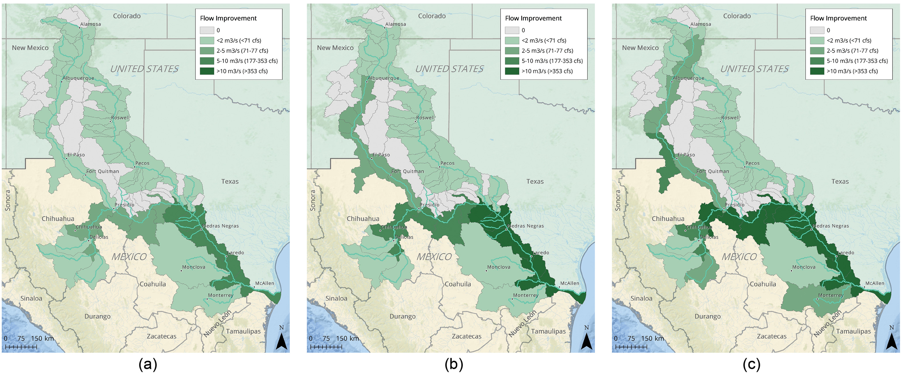
Step 3: Comparison of Potential Water Savings with Environmental Flow Gaps

To demonstrate the feasibility of environmental flow restoration strategies, we have focused our initial assessment of potential irrigation savings on 12 HUC8s within New Mexico that are proximate to our highest priority river segment, which runs from Albuquerque to San Marcial, New Mexico. We focus on these nearby HUC8s because we want to minimize any evapotranspiration losses in conveying water savings into our priority river segment.

In this segment of the Rio Grande, irrigation water is managed by the Middle Rio Grande Conservancy District. A portion of the district’s overall irrigation supply is stored in El Vado Reservoir on the Rio Chama (tributary to the Rio Grande upstream of Albuquerque, see Fig. 1). We assume that water saved by reducing irrigation demands can be temporarily stored in El Vado Reservoir for release during July–October and protected as environmental flow through the entire length of our targeted river segment from Albuquerque to San Marcial.

As specified in Table 1, a volume of

21 \times 10^{6} m^{3}

(

17,025 acre / ft

) per year in reduced irrigation consumption is needed to fill the environmental flow gap at Albuquerque, and

35 \times 10^{6} m^{3}

(

28,375 acre / ft

) per year is needed at San Marcial. As indicated in Figs. 5 and 6 and Table 2, the environmental flow gap at Albuquerque can be fully met by reducing irrigation by a little more than 20% across the HUC8s upstream and proximal to Albuquerque. However, fully filling the gap at San Marcial will require implementation of additional water-conserving strategies, or a relaxation of the constraints we imposed on our optimizations, as addressed in the “Discussion” section.

Table 2. Potential water savings from reduced irrigation consumption

HUC ID	HUC Name	$- 10 %$	$- 20 %$	$- 30 %$
13020101	Upper Rio Grande	1.84	3.92	6.23
13020102	Rio Chama	0.35	0.73	1.14
13020201	Rio Grande–Santa Fe	1.98	4.23	6.69
13020202	Jemez	0.04	0.08	0.12
13020203	Rio Grande–Albuquerque	2.52	5.41	8.60
13020204	Rio Puerco	0.06	0.12	0.18
13020211	Elephant Butte Reservoir	2.54	5.45	8.66
Total		9.33	19.92	31.62

Note: The volumes of potential water savings in each HUC8 when irrigation consumption is reduced by 10%–30% are indicated in million cubic meters ( $10^{6} m^{3}$ ); water savings in 5 of 12 HUC8s assessed were negligible and are therefore not listed here. These results indicate that a little more than 20% reduction in irrigation consumption would be sufficient to fill the environmental flow gap ( $21 \times 10^{6} m^{3}$ ) at Albuquerque, but a 30% reduction in irrigation is insufficient to fill the $35 \times 10^{6} m^{3}$ gap at San Marcial.

Step 4: Assessing Optimization Strategies for Attaining Needed Irrigation Savings

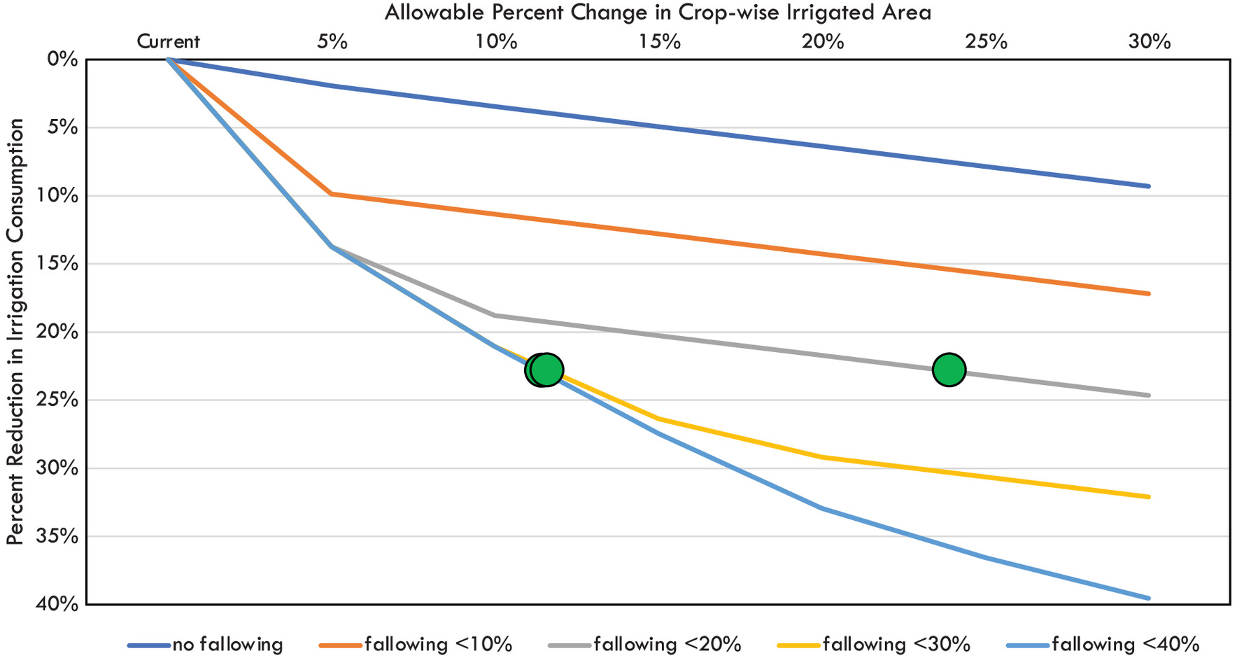
The final step in our assessment was to more deeply explore the potential to realize the requisite volume of irrigation savings at Albuquerque by optimizing the crop mix in the proximate HUCs and temporarily or permanently fallowing some portion of farmland near the Rio Grande. Importantly, we note that none of these optimization scenarios decrease net profits within any HUC8. We have estimated net profits for each crop type in each HUC8 using methods described in Richter et al. (2022) and did not allow the aggregate profit in any HUC8 to decline in our optimizations. The volumes of potential irrigation savings across the HUC8s are illustrated in Fig. 7. The optimization scenarios span a range (5%–30%) that each crop’s irrigated area is allowed to change in the optimizations, as well as a range of fallowing from 0% to 40%.

Fig. 7. Potential water savings from crop shifting and fallowing. The potential irrigation savings across the seven HUC8s are shown here, under fallowing options ranging from 0% to 40%. The allowable percentage change in crop-wise irrigated area represents the percentage to which any individual crop can be reduced in area in the optimization runs. The green dots depict the optimization runs in which 23% irrigation savings is attained, which is sufficient to fill the environmental flow gap at Albuquerque.

As suggested by Fig. 7 and Table 2, the needed water-savings volume of

21 \times 10^{6} m^{3}

per year—equating to a reduction in irrigation of 23% and an average increase of

{2.2 m}^{3} / s

(

{81 ft}^{3} / s

) in the river during July–October—can be attained under a variety of options. We note that the environmental flow gap at Albuquerque cannot be filled completely if fallowing is not included (Fig. 7; Table 3, Scenario 1). However, by fallowing or shifting away from alfalfa into other hays (Table 3, see Scenario 2), or by reducing the area of both alfalfa and other hays (Table 3, see Scenario 3), the needed water savings can be achieved. The revenue lost from reduced alfalfa and other hays can be fully recovered with addition of green chili pepper production, due to the much higher (

\sim 20 x

) net revenues associated with chili peppers.

Table 3. Optimized crop and fallowing mixtures

Scenario ID	Scenario description	Alfalfa	Barley	Corn	Oats	Other hay	Potatoes	Spring wheat	Green chili peppers
Current	Existing conditions	13,701 (77%)	259 (1%)	494 (3%)	186 (1%)	2,357 (13%)	171 (1%)	176 (1%)	309 (2%)
Scenario 1	No fallowing	Cannot achieve 23% water savings
Scenario 2	Fallowing area $< 18 %$ ; allow crop area change $< 29 %$	8,605 (48%)	0 (0%)	0 (0%)	186 (1%)	3,317 (19%)	206 (1%)	176 (1%)	2,150 (12%)
Scenario 3	Fallowing area $< 27 %$ ; allow crop area change $< 12 %$	11,593 (65%)	0 (0%)	10 (0%)	186 (1%)	1,687 (9%)	182 (1%)	176 (1%)	808 (5%)

Note: The crop and fallowing mixtures that can attain 23% water savings annually are summarized here (based on average water use during 2000–2019). Crop area is reported in both hectares and percent of total irrigated area.

Discussion

The RGRB hydroecological integrity has been greatly diminished since the 1880s, primarily due to severe flow depletion for irrigation, which accounts for 83% of water consumed for human purposes in the basin. However, important intermittent patches of habitat remain—a “string of ecological pearls”—that require environmental flow restoration to support imperiled and other native species dependent upon the RGRB ecosystem. This study serves as an initial feasibility assessment that explores both the volume of needed flow restoration in a critically important reach of the Rio Grande between Albuquerque and San Marcial, New Mexico, as well as potential on-farm strategies that can be deployed to generate requisite water savings.

Environmental flow restoration efforts along the RGRB in New Mexico have included programs that temporarily lease water rights or financially incentivize farmers to temporarily fallow their crops. These pilot fallowing programs have been designed to benefit both endangered species and farmers’ needs during drought by providing water for species as well as funds for farmers that supplement their farm income. These pilot efforts have produced very important short-term boosts in low flows during critically dry years that have been particularly important in sustaining silvery minnow populations and, if brought to scale, could have long-term benefits. Our findings suggest that additional significant and long-term environmental flow benefits can be achieved by reducing the irrigation required to produce water-intensive crops such as alfalfa and grass hay. Our exploration of optimized farm strategies has been bounded by practicality. We have constrained our optimization in important ways, including a requirement that farmers in each subbasin would continue to earn the same or greater levels of net profit, and that limits would be set on the degree to which any existing crop’s irrigated area could be reduced, thereby minimizing supply chain disruptions. Richter et al. (2022) discuss the need for funding incentives and technical assistance to encourage adoption of crop-shifting and fallowing strategies in the western United States. By demonstrating how such strategies could be implemented in the RGRB basin in an incremental fashion—such as by focusing on high-priority river segments and proximate farms—we hope to shed light on realistic pathways forward.

However, we recognize that farmer adoption of crop-shifting or fallowing strategies will depend upon additional factors beyond income stability and financial aid for crop transitioning. For example, discussions with the Middle Rio Grande Conservancy District suggest that farmers will be reluctant to shift to crops such as green chili peppers that require substantial manual labor during harvests, due to a severe shortage in farmworker availability in recent years (J. Casuga and C. Ish, personal communication, 2023). Market competition with chilis imported from Mexico may also dissuade increased production along the Rio Grande (Cook 2023). Increasing chili production may also require development of a local processing facility to enhance the marketability of chilis grown in this area. A primary purpose of this paper is to help stimulate a conversation about water-conserving farm strategies that are most feasible and acceptable to farmers. Our next steps will include deeper engagement with farmers in the region as well as helping implement field research on the water consumption of various alternative crops, including some that have not been produced in this area previously.

Importantly, any reductions in overall irrigation consumption will also greatly aid New Mexico’s efforts to meet its interstate Rio Grande Compact obligations to deliver a required volume of water to Texas each year. In recent years, New Mexico has struggled to fully meet that obligation (Grover 2021). During discussions with staff at both the Middle Rio Grande Conservancy District and the New Mexico Interstate Stream Commission (P. Pegram and G. Haggerty, personal communication, 2023), water management officials in the state are highly motivated to find ways of reducing water consumption and are receptive to ideas for meeting interstate Compact obligations as well as endangered species requirements. Meeting environmental flow goals can align with Compact goals if environmental flow enhancement results in increased water deliveries to Texas.

While our analysis suggests that environmental flow needs at the upstream end of our target river reach at Albuquerque can be met with a combination of crop shifting and fallowing, we were unable to completely fill the environmental flow gap further downstream at San Marcial using these strategies alone, under our assumed constraints. Supplemental strategies or relaxation of the constraints we have used in our optimizations will need to be deployed to reach environmental flow goals at San Marcial.

Supplemental Materials

File (supplemental_materials_jwrmd5.wreng-6278_richter.pdf)

Download
256.67 KB

Data Availability Statement

All data and models that support the findings of this study are available from the corresponding author upon reasonable request.

Acknowledgments

Jaime Rivera and Martina Floerke of Ruhr University Bochum provided water-use data from the WaterGAP model. Kyle Davis, Gambhir Lamsal, and Landon Marston acknowledge support by the United States Department of Agriculture National Institute of Food and Agriculture (Grant No. 2022-67019-37180).

References

Autobee, R. 1994. The Rio Grande project. Denver: Bureau of Reclamation.

Abstract

Introduction

Water Infrastructure and Policy Development

Headwaters Irrigation Phase

International Water-Sharing Agreement and Large Reservoir Construction in the United States

Reservoir Development in Mexico

Interstate Water-Sharing Agreement

International Cooperation to Build Reservoirs and Share the Lower River

Effects of Water-Sharing Agreements on Flow Regime

Data and Methods

Quantification of Environmental Flow Needs and Gaps

Hydrological Model Development

Assessing Potential Irrigation Savings from Crop-Shifting and Fallowing

Results

Step 1: Assessing Flow Depletion Using Basin-Wide Hydrologic Model

Step 2: Evaluating Potential Flow Improvement from Reduced Irrigation

Step 3: Comparison of Potential Water Savings with Environmental Flow Gaps

Step 4: Assessing Optimization Strategies for Attaining Needed Irrigation Savings

Discussion

Supplemental Materials

Data Availability Statement

Acknowledgments

References

Information

Published In

Copyright

History

ASCE Technical Topics:

Authors

Affiliations

Metrics

Citations

Download citation

Figures

Other

Share

Copy the content Link

Share with email

Share

Request Username

Create a new account

Change Password

Password Changed Successfully

Verify Phone

Congrats!