How to Model an Intermittent Water Supply: Comparing Modeling Choices and Their Impact on Inequality
Publication: Journal of Water Resources Planning and Management
Volume 150, Issue 1
Abstract
Intermittent water supply (IWS) networks have distinct and complicated hydraulics. During periods without water supply, IWS networks drain, and consumers rely on stored water; when supply resumes, pipes and consumer storage are refilled. Draining, storage, and filling are not easily represented in standard modeling software. We reviewed 30 ways modelers have represented the hydraulics of IWS in open-source modeling tools and synthesized them into eight distinct methods for quantitative comparison. When selecting methods, modelers face two critical choices: (1) whether to ignore the filling phase, and (2) how to represent consumers as attempting to withdraw their demand: as fast as possible (unrestricted), as fast as possible until a desired volume is received (volume-restricted), or just fast enough to receive a desired volume by the end of supply (flow-restricted). We quantify these choices’ impact on consumer demand satisfaction (volume received/volume desired) and inequality using three test networks under two supply durations, implemented in two different hydraulic solvers (EPANET and EPA-SWMM). Predicted inequality and demand satisfaction were substantially affected by the choice to represent consumer withdrawals as unrestricted, volume-restricted, or flow-restricted, but not by the specific implementation (e.g., three different flow-restricted methods agreed within 0.01%). Volume-restricted methods predict wider inequalities than flow-restricted methods and unrestricted methods predict excessive withdrawal. Modeling filling delayed water provision unequally, reducing the volume received by some consumers (by ), especially where water supply is brief. All else being equal, we recommend using volume-restricted methods, especially when modeling system improvements, and including the filling process when studying inequalities.
Practical Applications
Understanding how water distribution networks perform is complicated, particularly when the network is operated intermittently. Pipes in intermittent networks periodically fill up, supply water, and then drain, forcing consumers to adapt, e.g., by storing water. Intermittent networks represent about 20% of the world’s water pipes, but there are not yet standardized, accessible methods for practitioners and utilities to model the key features of intermittent networks by using or adapting off-the-shelf hydraulic software. Previous methods of adapting hydraulic software for IWS networks disagree on two key choices: how consumers behave and whether to ignore the initial filling of pipes. We quantitatively compare how these varied choices affect the resultant hydraulic predictions. First, we find that when consumers are assumed to fill their storage as fast as they can (volume-restricted), water delivery is less equal than if consumers are assumed to withdraw slower (flow-restricted). Second, we found that including pipe filling delays water supply and magnifies predicted inequalities. Accordingly, we recommend that modelers carefully select methods that reflect how consumers behave in their context. We provide accessibly packaged Python code to enable other hydraulic modelers to efficiently compare, extend, and/or adopt the compared intermittent modeling methods.
Introduction
Water distribution networks (WDNs) are typically designed to operate continuously, yet many utilities struggle to provide as much water supply as their consumers want (Galaitsi et al. 2016). Whether due to water scarcity, power shortages, lack of funds to expand network capacity, ineffective operation strategies, and/or deteriorated infrastructure causing leaks, many WDNs are operated intermittently, i.e., frequently less than (Simukonda et al. 2018; Vairavamoorthy et al. 2007). With increasing populations, urbanization, and climate change impacting water resources, the persistence of intermittent water supply (IWS) networks—if not their proliferation—is expected, especially in the Global South (Galaitsi et al. 2016; Vairavamoorthy et al. 2008).
The persistence of IWS is problematic due to its increased risk of contaminant intrusion, accelerated deterioration of network assets, and unequal restrictions on consumer withdrawals (Guragai et al. 2017; De Marchis et al. 2011; Taylor et al. 2018). These drawbacks of IWS threaten progress toward global water goals such as Target 6.1 of the United Nations’ Sustainable Development Goals (SDGs), which aims for “universal and equitable access to safe and affordable drinking water for all” (WHO and UNICEF 2021). Thus, improving IWS service quality and equality is of high interest to WDN designers, operators, regulators, policymakers, and researchers.
To identify opportunities to improve IWS service quality and equality, several IWS researchers have coupled hydraulic modeling with optimization techniques (e.g., Gullotta et al. 2021; Ilaya-Ayza et al. 2017). Studies using modeling are cheaper and faster than physical experiments, enabling orders of magnitude more exploration of network deficiencies and their causes (Walski et al. 2003). But for IWS optimizations to provide meaningful and applicable insights, the hydraulic model they rely on must be sufficiently representative of the behavior of real IWS systems.
Established hydraulic modeling software tools were created to model continuous water supply (CWS) networks [e.g., EPANET (Rossman et al. 2020)] and, unfortunately, did not include native options for modeling the salient features of IWS. To overcome this limitation, researchers have modeled IWS by modifying existing software or creating their own (Sarisen et al. 2022). These IWS modeling efforts vary substantively in two critical choices: whether to ignore the filling phase and how to represent consumer withdrawals. Variations in these modeling choices lead to disparate, at times even conflicting, predictions about demand satisfaction and inequality.
A recent summary of IWS modeling methods found 21 studies that proposed or utilized modeling methods for IWS (Sarisen et al. 2022). Their work highlights that despite the proliferation of IWS modeling methods and choices, there are no quantitative comparisons of these methods and their network predictions. Building on their important work, we aim to enable IWS modelers to make informed choices that match their modeling purpose and contexts. To do so, we
•
critically reviewed and qualitatively contrasted existing methods of modeling IWS that use the open-access software EPANET or EPA-SWMM, synthesizing 30 studies based on their choices about consumer withdrawals and network filling, and
•
quantitatively compared these methods and the impact of their assumptions about withdrawals and filling on predicted consumer demand satisfaction and inequality.
A Critical Review of Modeling Choices in IWS
In this section, we qualitatively and critically review two impactful choices that IWS modelers make when modeling IWS networks: how to model consumer withdrawal and which phases of the IWS cycle to model.
Modeling IWS Consumer Withdrawal
Typically, IWS networks are designed to run continuously but are operated intermittently. To intermittently supply consumers with as much water as they desire (i.e., to satisfy their demand), flow rates in intermittent networks need to be higher than during CWS. Flows during IWS are, therefore, often higher than the designed capacity, which usually leads to low pressures (Vairavamoorthy et al. 2007), which can affect consumer withdrawals. Pressure-driven analysis (PDA), a tool developed to represent consumer withdrawals during unexpected pressure deficiencies in CWS, has been frequently repurposed to model IWS networks, which are often pressure-deficient. PDA provides a representation of how consumer withdrawal rates at a given node depend on the available pressure at that node. Many formulations for PDA have been proposed; we follow the majority of the IWS modeling methods we reviewed for this study and use the pressure-dependent withdrawal formulation of Wagner et al. (1988):where = consumer’s pressure-dependent withdrawal rate; = pressure at the demand node; = consumer’s desired withdrawal rate, which we define as the flow that would flow that would allow them to satisfy their demand within the supply duration. For example, if a consumer demands and is supplied for , their desired flow rate would be to satisfy 100% of their demand. , , and collectively represent the resistance of the service connection between the node and the consumer, where = minimum pressure required to start withdrawing; and = (desired) pressure at which the consumer can withdraw their desired demand .
(1)
Complicating pressure-dependent withdrawals [Eq. (1)], IWS consumers typically store water for use between supply periods in containers or tanks (Fontanazza et al. 2007; Kumpel et al. 2017), which may be connected to float valves (Criminisi et al. 2009) and/or pumps (Meyer et al. 2021b). Yet only some IWS modelers chose to include consumer storage in their methods; including pumps and/or float valves is even less common (Campisano et al. 2019a; Gullotta et al. 2021). In all reviewed modeling methods, modelers have chosen to represent the nuances of IWS consumers using one of three distinct assumptions that can be summarized bywhere = cumulative volume received by a consumer in a supply cycle; and and = assumed restrictions (or lack thereof) on withdrawal rate and received volume , respectively. Modelers chose and to represent consumer withdrawal in one of the following three ways:
(2a)
(2b)
•
Unrestricted: consumers attempt to withdraw as fast as network hydraulics permit, i.e., always equals ( and ).
•
Volume-restricted: consumers attempt to withdraw as fast as hydraulically permissible () until they receive the total volume of water they desire, ().
•
Flow-restricted: consumers attempt to withdraw just fast enough to meet their demand ( and ).
An initial perspective on these withdrawal types was presented at the Water Distribution Systems Analysis and Computing and Control in the Water Industry (WDSA-CCWI 2022) conference (Abdelazeem and Meyer 2022). We explore each of these withdrawal representations after summarizing the second major choice facing IWS modelers: which phases of IWS to include.
Modeling the Phases of IWS
IWS networks are characterized by cyclic phases:
•
filling (initial charging), where the partially full and empty pipes are filled,
•
pressurized supply, where supply from the source is maintained and network pipes are fully pressurized, and
•
draining, where supply is stopped, and pipes are drained partially or fully by leaks and/or consumer demand.
Although the hydraulics during pressurized supply are similar to CWS, apart from consumer withdrawals, the filling and draining phases are more complicated and computationally expensive to model (Sarisen et al. 2022). Accordingly, most published methods of modeling IWS have ignored the filling and draining phases (Table S1 ), focusing instead on the nuanced behavior of IWS consumers.
In addition to classifying IWS modeling methods based on consumer withdrawal assumptions, we also classified methods based on their choice to either model the pressurized phase only or to additionally include the filling phase. During our 2022 literature review, we found only two methods that included draining: Mohan and Abhijith (2020) studied the draining of a four-pipe undulating network, but was subsequently critiqued for not conserving mass or momentum (Meyer and Ahadzadeh 2021). Gullotta et al. (2021) created a network model in EPA-SWMM, citing other papers for their modeling methodology, but their paper and its citations did not include draining details; accordingly, we omitted both papers and draining itself from our comparison. More recently, Ceita et al. (2023) also included draining in their EPA-SWMM model, however, a comparison of modelling methods for draining and their impact is left for future work.
Modeling Pressurized IWS in EPANET
The earliest IWS modeling methods ignored the filling and draining phases to be able to use CWS hydraulic modeling software, namely EPANET. These methods approximated common hardware components used by IWS consumers, e.g., tanks/containers, float valves, and pumps, and mimicked their withdrawal behavior by adding artificial (i.e., not physically present in the network) elements to skeletonized demand nodes. We replicate these open-source methods as a way of quantitatively exploring the impact of all three consumer withdrawal assumptions on predicted consumer satisfaction and equality.
Unrestricted Methods
Unrestricted methods of modeling IWS aim to simulate consumers who leave their taps fully open to withdraw as much water as possible—even in excess of their demand—to fill their storage containers (Mohapatra et al. 2014). Accordingly, consumers are assumed to always withdraw at the highest hydraulically permissible rate [Eq. (1)], without imposing an external restriction on flow rate or volume [ and , Eq. (2)]. Unrestricted methods model IWS consumers by adding artificial reservoirs—representing storage—to each demand node with the reservoir’s elevation raised above their respective demand nodes by to prevent flow when pressures are too low [, Eq. (2)] (Mohapatra et al. 2014). A pipe with a check valve (CV) connects the demand node to the artificial reservoir, with the pipe’s resistance adjusted to mimic the pressure dependence (hydraulic resistance) in Eq. (1) (details are given in Text S1 ). The assumptions of unrestricted withdrawals correspond well with consumers who have extremely large storage containers and/or allow storage containers to overflow when full.
Volume-Restricted Methods
Similar to unrestricted methods, volume-restricted methods assume IWS consumers withdraw water rapidly for storage [i.e., , Eq. (2)], but distinctly assume that consumers desire a finite demand volume each supply cycle (). is typically related to, but not usually equivalent to, the storage capacity of the consumer’s tank/containers. Thus, consumer withdrawals are affected by pressure [Eq. (1)], but withdrawals are assumed to stop once consumers have received their desired volume, i.e., filled their storage [ in Eq. (2)].
Volume-restricted withdrawal was proposed by Batterman and Macke (2001) for modeling IWS in EPANET. This method, later extended by Taylor et al. (2019), proposes the addition of an artificial tank to each demand node whose volume is . A check-valved pipe connects the demand node to the tank; the pipe’s major friction losses are adjusted to simulate friction losses in the secondary network [Eq. (S5 )] and the tank is raised above the demand node’s elevation by . With this formulation, flow into the artificial tank depends on the tank’s water level. Sivakumar et al. (2020b) noted that IWS consumer tanks typically fill from the top. Accordingly, they proposed the addition of a pressure-sustaining valve (PSV) upstream of the tank, maintaining atmospheric pressure to ensure that the filling rate is independent of the water height in the tank.
Flow-Restricted Methods
Flow-restricted methods assume that each IWS consumer desires a certain maximum flow rate () and even if provided with more than sufficient pressure (), their withdrawal does not exceed [i.e., , Eq. (2)]. In the context of an IWS, where consumer storage is common, this implies that consumers are either consciously restricting their withdrawal rate or an external restriction (e.g., control valves) is imposed. Flow-restricted methods impose no explicit restrictions on the total volume consumers can receive [i.e., , Eq. (2)]; however the total volume consumers can receive is usually implicitly restricted in the method’s definition of (often taken as , therefore limiting to if ).
Flow-restricted methods were originally proposed to perform PDA before native PDA options were available in common hydraulic solvers (e.g., EPANET). These methods modified EPANET by adding flow-control valves (FCVs) to limit withdrawal rates to . Jinesh Babu and Mohan (2012) added FCVs to pressure-deficient demand nodes and connected each of them to an artificial reservoir. Although Jinesh Babu and Mohan (2012) assigned negligible resistance to the artificial pipe (connecting the demand node and reservoir), which causes withdrawal to increase rapidly from zero to when , Gorev and Kodzhespirova (2013) added resistance to the artificial pipe to mimic the pressure dependence [Eq. (1)] through the minor loss coefficient [Eq. (S4 )]. Alternatively, Rossman (2007) suggested using emitters instead of reservoirs to simulate pressure-dependent demand [Eq. (1)] by adjusting the emitter coefficient and exponent; Abdy Sayyed et al. (2015) applied this approach to analyze pressure-deficient networks. Details on each method’s implementation are given in Text S1 and Table S2 . EPANET’s version 2.2 later introduced a PDA option (Rossman et al. 2020) allowing for native pressure-dependent demands [Eq. (1)].
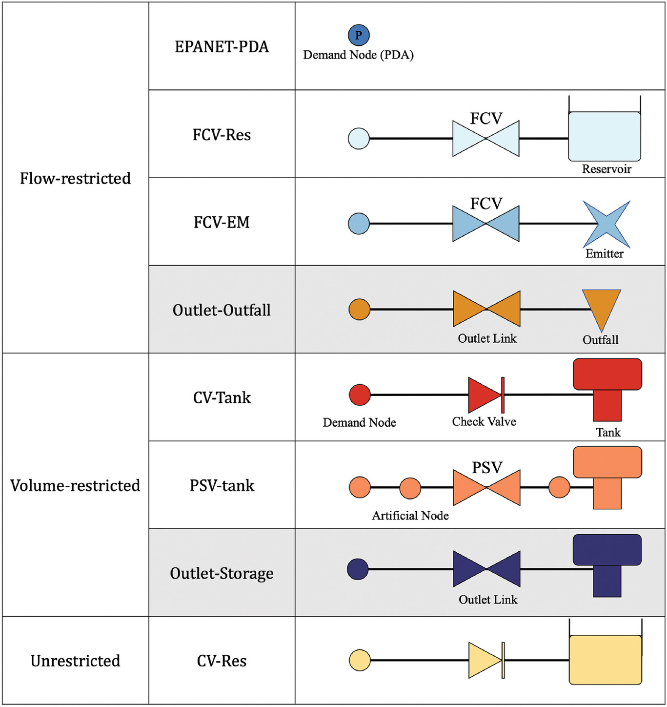
Where authors used the same characteristic artificial elements (e.g., FCV upstream of an emitter) to produce equivalent hydraulic behavior, we include only one such method—excluding for the sake of clarity and brevity methods that improve computational convergence or efficiency. Accordingly, we include one unrestricted method as detailed by Mohapatra et al. (2014), denoted CV-Res, two volume-restricted methods, proposed by Batterman and Macke (2001) and Sivakumar et al. (2020b) and denoted, respectively, as CV-Tank and PSV-Tank, and three flow-restricted methods: a reservoir-based method, FCV-Res, as detailed by Gorev and Kodzhespirova (2013), an emitter-based method, FCV-EM, as detailed by Abdy Sayyed et al. (2015), and EPANET’s native PDA option, EPANET-PDA. Fig. 1 depicts these methods and their implementation for a typical demand node in EPANET.
Modeling the Filling Phase with EPA-SWMM
Unlike pressurized IWS methods, some filling methods implemented customized models, whereas others adapted existing software. Customized models have solved versions of the continuity and momentum equations to model filling and/or draining using the method of characteristics (de Marchis et al. 2011), the backward difference method (Mohan and Abhijith 2020), and the Preissman slot (Lieb et al. 2016). Customized methods offer greater flexibility in their construction, but at the cost of accessibility and reproducibility, especially when models and/or validation data are not made available. A promising alternative to customized models has been modeling IWS using open-source software like EPA-SWMM. In the interest of accessibility and comparability with pressurized IWS methods, we limit our comparison to methods that use EPA-SWMM.
Reviewed filling methods modeled consumer withdrawals as flow-restricted or volume-restricted; we found no filling methods with unrestricted consumer withdrawals. Kabaasha (2012) proposed a SWMM-based method that models flow-restricted consumers using the outlet and outfall elements native to SWMM. For each demand node, an outlet link—analogous to a FCV—is added connecting the node to a free outfall. The pressure dependence [Eq. (1)] is then defined as a rating curve, relating outlet flow (limited to ) to depth (pressure) at the demand node. Campisano et al. (2019b) employed a similar approach and validated their method against measured data. We adapted Campisano et al.’s (2019b) method to represent flow-restricted SWMM methods and denote it as Outlet-Outfall (Fig. 1).
Segura (2006) proposed a volume-restricted method of modeling the filling of IWS networks using outlet links and storage nodes—analogous to tanks (thus represented by EPANET’s tank symbol in Fig. 1). Later, Campisano et al. (2019a) used control rules to model the gradual closure of a tank’s float valve, gradually reducing the inflow to the tank. Because tanks in EPANET close rapidly once they become full, we adapted Campisano et al.’s (2019a) method for comparability with EPANET volume-restricted methods (e.g., CV-Tank), and denote it as the Outlet-Storage method. The Outlet-Storage method uses control rules to rapidly stop flow into the tank by switching off the outlet link once the tank becomes full, similar to the CV-Tank method. Although some volume-restricted SWMM methods modeled consumer usage during supply (e.g., Gullotta et al. 2021), most pressurized EPANET methods and flow-restricted SWMM methods do not, and thus we omitted consumer use. The storage nodes are connected to the demand nodes using an outlet link whose rating curve simulates the head-flow relationship in Eq. (1).
For both Outlet-Outfall and Outlet-Storage methods, the following procedures were performed in order to produce convergent results that are comparable to EPANET results. Following Dubasik (2017), we defined pipes using SWMM’s force main geometry, which uses the Hazen-Williams (or Darcy-Weisbach) friction model when the pipe is pressurized. Thus, head losses calculated by EPA-SWMM after pressurization matched EPANET. We also followed Pachaly et al.’s (2020) recommendation of artificial spatial discretization (ASD) when modeling pipe filling in SWMM, where a real pipe is divided into smaller segments to produce more stable results. A spatial discretization with a maximum length of 10 m was selected as a compromise between model detail and computational cost. Time steps from 10 to 0.1 s were tested; time steps equal to or lower than 1 s provided virtually identical results, and thus 1 s was used.
EPA-SWMM provides two options for solving conduits that are pressurized, EXTRAN and Slot (an implementation of the Preissman slot). Although Pachaly et al. (2020) recommended the slot surcharge method, friction losses calculated by the slot and EXTRAN methods were substantially different (in SWMM version 5.2) due to the large slot width. We used the EXTRAN surcharge method for better comparability with EPANET methods. Lastly, nodes were assigned a negligible cross-sectional area () and set to flood (surcharge depth) at an arbitrarily high value (i.e., 100 m) to enable network pressurization without nodal overflows.
Quantitative Methodology
Each of the eight selected modeling methods were applied to three networks of different sizes and elevation profiles. Network 1 was adapted from Campisano et al. (2019b), Network 1 is characterized by steep slopes (range of 1%–23%) (Fig. S1 shows the elevations) and 38 demand nodes supplied by a reservoir (level assumed to be 30 m above the network’s highest node). Networks 2 and 3 have gentler slopes and represent the WDNs in Pescara and Modena, Italy, respectively. These networks were described in detail by Bragalli et al. (2012); Network 2 has 64 demand nodes supplied by three reservoirs, and Network 3 has 245 demand nodes supplied by four reservoirs. EPANET and EPA-SWMM input files for each network are shared in this paper’s data repository. The results presented subsequently are for the largest, most complex of these networks (Network 3). Results for Networks 1 and 2 are presented in the Supplemental Materials and discussed herein when substantially different.
To compare the distinct IWS modeling methods, we harmonized their assumptions. and vary widely depending on the relative elevation of consumer outlets, the resistance of their service connections, and the degree of skeletonization, e.g., consumers may have underground tanks () or roof tanks (). Accordingly, reviewed methods varied in their assumptions: Sivakumar et al. (2020b) used , whereas Campisano et al. (2019b) used of 5 and 10 m for their two networks, respectively. Unfortunately, little has been published about typical values of these thresholds in real IWS networks (Meyer et al. 2021a). To control for the impact of these assumptions, we set each method’s resistance to be equivalent to , , and (Tables S3 and S4 ), following Sivakumar et al. (2020b). An in-depth assessment of the impact of changing has been given by Sivakumar et al. (2020a).
Additionally, we assumed a consumer’s daily desired volume () was fixed for all methods and does not change with supply duration (), e.g., a consumer desires whether supply lasts for 4 or 12 h; however, consumers may still receive less than they desired (). We assumed the desired flow rate to be ; the resistance of the service connection was then determined by , , and as follows:
(3)
To explore a range of possible values for service connection resistances and supply durations, we compare all methods under two supply durations: 4 and . The service connection resistance was achieved differently by different methods, often through major or minor losses in artificial elements (Text S1 gives more details); our harmonized resistance values [Eq. (3)] allow these methods to be directly and meaningfully compared.
Input file preparation, simulation execution, and output file processing were performed in Python version 3.9.12. Simulation execution was timed through 1,000 repeated runs to compare the methods’ computational efficiency. EPANET-based simulations were executed using the Water Network Tool for Resilience (WNTR) package version 0.4.1 for Python 3 (Klise et al. 2017); EPA-SWMM-based simulations were executed using the PySWMM package (McDonnell et al. 2020).
To summarize each method’s predictions, the volumes received by consumers were transformed into a demand satisfaction ratio , the ratio of the volume received to the volume desired (). Evaluating the satisfaction ratio—also called supply ratio (Gullotta et al. 2021)—for individual consumers throughout the supply duration highlights inequalities in how fast they receive their demands. If the supply duration is unexpectedly cut short (e.g., power outage), the impact on consumers can be assessed using their satisfaction ratio at the time the supply is cut.
Quantitative Results and Discussion
Models of IWS Consumers Generalize to Three Types
We compared all six methods of modeling pressurized IWS (in EPANET) based on their predictions of how the network-averaged demand satisfaction ratio varies during the supply. We compared methods using two different supply durations, which created different pressure conditions in the network: the shorter supply duration increased consumers’ desired withdrawal rates, thus increasing flow rates and friction losses and decreasing pressures throughout the network (despite constant reservoir pressures). We summarize the methods’ predictions in the following subsections based on our classification of their withdrawal assumptions.
Flow-Restricted Methods
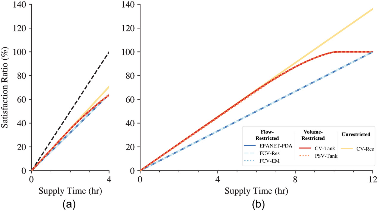
All three flow-restricted methods predicted a constant and restricted withdrawal rate, as expected. When consumers are provided with sufficient pressure (e.g., longer supply duration) [Fig. 2(b)], the consumer satisfaction rate was maintained at by the imposed flow restriction (just enough to satisfy demands by the end of supply). When pressures dipped below desired for at least some consumers, average consumer satisfaction follows a slope lower than (e.g., shorter supply duration) [Fig. 2(a)]. All three flow-restricted methods provided practically identical predictions under both supply durations (difference ), which was expected because we implemented each with the same assumptions about the minimum pressure, desired pressure, and desired flow. Despite the success of the two historical flow-restricted methods (FCV-EM and FCV-Res) in producing highly similar predictions to native PDA option in EPANET 2.2, EPANET’s PDA was two to three times faster in execution (Table S5 ), superseding the need for these historical methods.
Unrestricted Methods
The unrestricted method (CV-Res) predicted a constant withdrawal rate but at a higher slope (faster flows) than flow-restricted methods. Distinctly, because the unrestricted method is not bounded by the flow restriction , it overshoots the desired demand for all consumers when nodal pressures are higher than the desired pressure. For example, when Network 3 was simulated with a 12-h supply duration, the mean consumer satisfaction was 136% (nodal range: 109%–209%) corresponding to a mean pressure at consumer nodes of (nodal range: 11.9–43.7 m) (Fig. S6 ), highlighting the method’s sensitivity to the assumed desired pressure (here 10 m). Because consumer storage is not restricted in this method, consumers advantaged hydraulically—by elevation and/or proximity to the source—may be predicted to withdraw more than they can physically store or might want.
Unrestricted withdrawal was proposed for scenarios where the supply duration was insufficient for any consumer to satisfy 100% of their demand, and thus leads to unlikely predictions if the supply duration is sufficient for at least some consumers. Because we intend moving forward to explore the effect of withdrawal models on demand satisfaction, particularly as systems attempt to improve satisfaction, we did not explore this method further.
Volume-Restricted Methods
Volume-restricted methods predict initial withdrawal rates similar to unrestricted methods owing to their shared lack of flow restriction. This initial rate is dependent on network pressures and service connection resistance ; higher pressures and/or lower service connection resistances increase the range of withdrawal rates possible for consumers in the network. Thus, the difference in withdrawal rates between volume- and flow-restricted methods is more prominent in longer durations [Fig. 2(b)], and less prominent in shorter supply durations (which result in higher desired flow rates, and hence lower pressures) [Fig. 2(a)].
Uniquely, volume restricted methods predict time-varying withdrawal rates: average withdrawal rate decreases as consumer tanks become full [i.e., some consumers stop withdrawing, reducing the mean (Fig. 2)], which plateaus when all consumer tanks are full () [Fig. 2(b)]. Both volume-restricted methods (CV-Tank and PSV-Tank) predicted a similar mean consumer satisfaction (difference ) [Fig. 2(b)] as long as pressures in the network were relatively higher than the water depth in consumer tanks [here, as often, assumed to be (Meyer et al. 2021a)].
Given the homogeneity within flow- and volume-restricted methods’ predictions ( and 0.7%, respectively), we selected one representative method from each group to use in the following analysis for simplicity (EPANET-PDA and CV-Tank, respectively).
Impact of Consumer Withdrawal Model on Inequality
Many IWS networks have irregular and/or unreliable supply schedules and so in practice, water is not always supplied as long as planned (Galaitsi et al. 2016). Where the supply duration is shorter than expected/planned, flow-restricted (FR) and volume-restricted (VR) methods disagree on how much consumers will withdraw before the supply ends and on the degree of consumer demand satisfaction (e.g., Fig. 2). To demonstrate the importance of intermediate predictions, we visualize the distribution of consumer satisfaction ratios halfway through the 12-h supply duration (at 6 h) (Fig. 3).
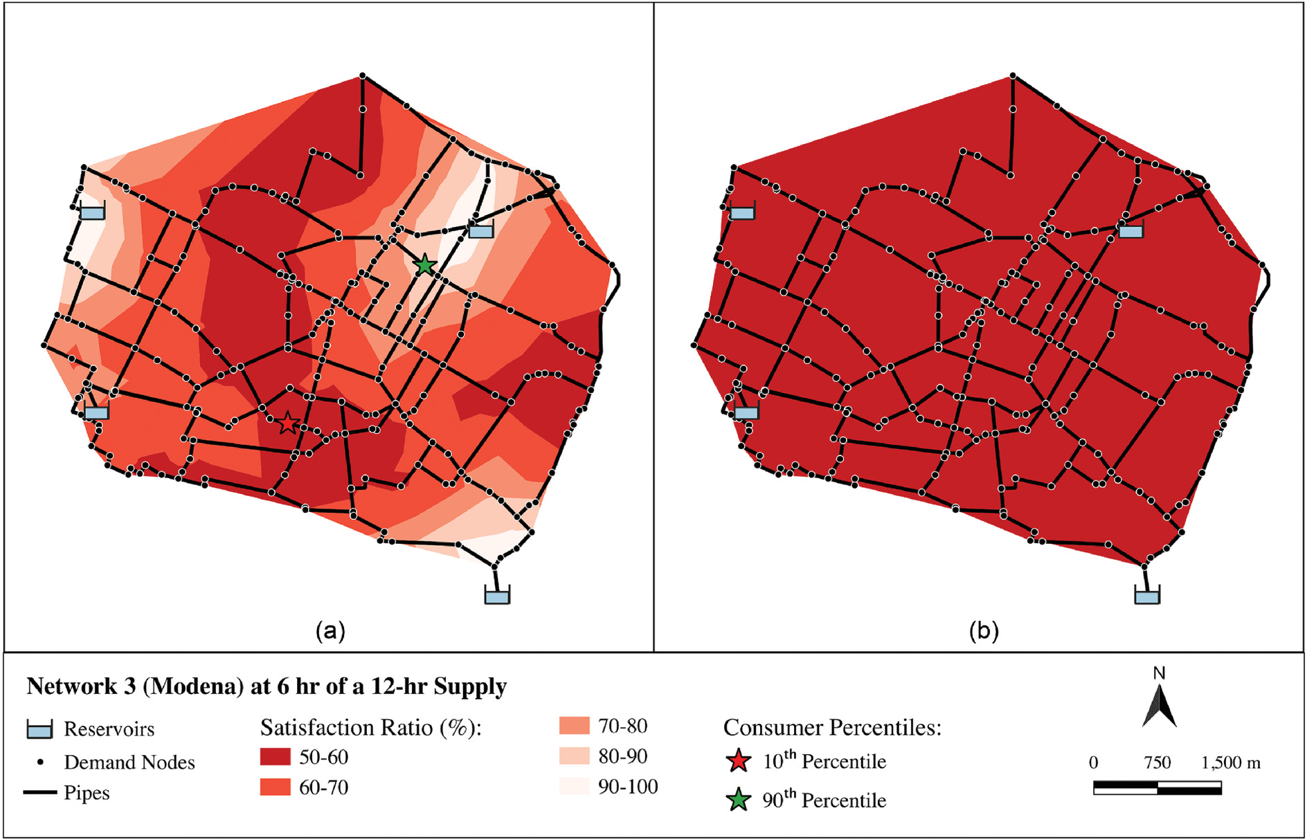
Halfway through the 12-h supply, VR methods predict an unequal distribution of demands: a few advantaged consumers (lightest) [Fig. 3(a)] have received 100% of their demand, whereas most consumers remain unsatisfied (). In this scenario, VR methods suggest that shortened supply reduces the service quality of a disadvantaged majority, but an advantaged minority remain well-supplied. In contrast, FR methods predict that all consumers in this scenario (where all pressures are ) will have received the same portion of their demand (), implying an equal sharing of the burden. The choice of withdrawal model strongly influences predicted demand satisfaction and equality during a shortened supply duration (e.g., due to water or power shortages).
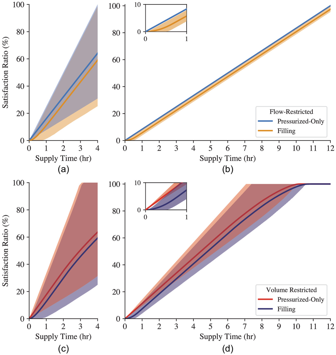
To understand the effects of shortened supply durations more broadly, we investigated the time evolution of the range of satisfaction ratios throughout the supply duration. In Fig. 4, we plot the mean satisfaction ratio (as a solid line) predicted by FR and VR methods (as in Fig. 2). Additionally, we represent the distribution of individual consumers’ demand satisfaction by the shaded area bounding the 10th- and 90th-percentile consumers (disadvantaged and advantaged, respectively).
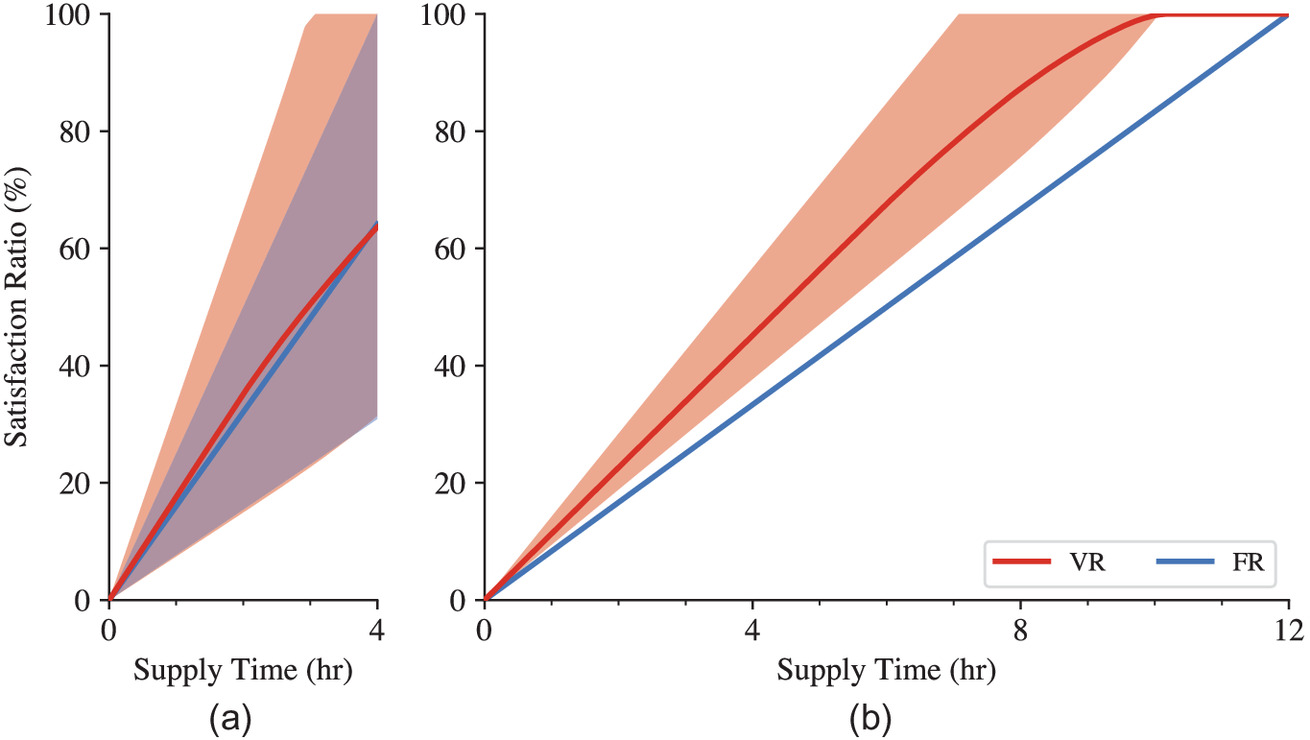
FR methods predict constant network flow rates and constant pressures throughout the supply duration. Thus, not only does the mean satisfaction ratio progress linearly, but so do the 10th- and 90th-percentile consumers (and all consumers). Hence if all pressures are higher than the desired pressure (e.g., in the 12-h supply duration), then the system is predicted to be perfectly equal: all consumers are predicted to satisfy their demand at the same rate [Fig. 4(b)]. Contrastingly, under the lower pressures of a 4-h supply, advantaged consumers (e.g., 90th percentile) are predicted to have enough pressure () to withdraw at the highest permitted rate (resulting, eventually in ), but disadvantaged consumers (e.g., 10th percentile) are predicted to withdraw at lower rates and satisfy less of their demands [Fig. 4(a)].
VR methods, in contrast, predicted a wide variance between consumers in both supply durations. The initial withdrawal rate of all consumers depends on pressure; it can be lower than desired when pressures are lower than desired (as in FR methods), but it can also be higher where the pressure is higher. Thus, VR consumers advantaged by elevation and/or source proximity are predicted to withdraw at higher rates than FR methods predict, allowing them to satisfy their demand earlier [e.g., 90th percentile after 7 h in Fig. 4(b)]. This enables the network to supply higher pressures to disadvantaged consumers later, hydraulically staggering demands. This staggering in VR methods is visible in the time evolution of the 10th-percentile consumer’s withdrawal rate, which accelerates after the 90th-percentile consumer is satisfied [e.g., after 6 h in Fig. 4(b)]. This uptick is also present, but less visibly, under a shorter supply duration, where network pressures are lower.
Differences in predicted inequalities (demand distribution) between FR and VR methods are caused by the central distinguishing assumption of FR methods, namely, that as pressure increases beyond the desired pressure, consumers’ withdrawal rates will not increase beyond . By design, FR methods only capture disadvantages due to low pressure but were not intended to capture advantages due to high pressure, and thus do not. This may limit the utility of FR methods where pressures are expected to rise above the desired pressure, for example, during the transition from intermittent to continuous supply. If FR methods are used to model this transition, they exclude the possibility that consumers may try to withdraw faster than expected by the modeler (i.e., ). Underpredicting consumer withdrawals may lead to undersized pipes and insufficient network pressures. Thus, where pressures are expected to rise above the desired threshold for at least some consumers, including during the transition to continuous supply, our findings suggest that volume-restricted methods more fully capture the plausible range of consumer behaviors and are therefore recommended.
Impact of Modeling the Filling Phase of IWS
Choosing to model the filling phase delayed the predicted demand satisfaction for all consumers, as expected. For FR methods, the delay due to filling meant that no consumer was predicted to receive 100% of their demand. This occurs because we computed the desired flow without considering filling and because FR consumers cannot increase their withdrawal rate to compensate for the delay [Fig. 5(a)]. Unlike their pressurized-only counterparts, FR methods that included filling predicted varied consumer satisfaction, even under high pressure, because filling delays are not experienced equally by consumers. Advantaged consumers experienced shorter filling delays (time before water reached their node ), whereas for the disadvantaged 10th-percentile consumers, water did not arrive for 37 and 28 min under the 4-h [Fig. 5(a)] and 12-h [Fig. 5(b)] supply, respectively. For advantaged consumers, the short delay had little impact on their satisfaction; they were predicted to receive of their demand. The longer delay of disadvantaged consumers, in contrast, reduced their total predicted withdrawals by 18.2% and 4.5% in the 4- and 12-h supply. Thus, modeling the filling phase reduced the effective supply duration unequally for each consumer. This suggests that the effects of filling under the assumptions of FR could be represented by assuming pipes begin full and instead reducing the supply duration to account for the expected filling delay, which could be estimated based on consumer-specific parameters (e.g., elevation or distance to source).
Modeling filling in VR methods, like in FR methods, introduced delays that disproportionately impacted disadvantaged consumers; disadvantaged consumers had to wait longer before they could start withdrawing. Unlike FR methods, however, VR methods predicted that some consumers can still satisfy 100% of their demand in the 12-h supply duration, despite the filling delay (range: 2–29 min), because flow rates are not restricted to and because demands can be staggered. In the 4-h supply duration, advantaged consumers were still predicted to recieve still received 100% of their demand—but 2 min later—whereas disadvantaged consumers received 20.5% less than predicted without considering filling due to a delay of . Because advantaged consumers in VR methods can withdraw at rates higher than the desired flow rate—which leads to higher friction losses—the predicted filling delay experienced by disadvantaged consumers is longer when consumers are modeled as VR rather than FR (delay versus ).
For FR and VR methods that include filling, predicted filling delays for advantaged and median consumers were relatively insensitive to supply duration and the choice of withdrawal model (). Conversely, predicted delays for disadvantaged consumers varied meaningfully with supply duration and withdrawal model; delays were longer under shorter supply durations and slightly longer when modeling consumers as volume-restricted. Regardless of the choice of consumer model, choosing to model the filling phase disproportionately reduced the predicted service quality (delivered pressure and volume) of disadvantaged consumers, suggesting that pipe filling exacerbates the inequalities exacerbating the inequalities of IWS. Additionally, the relative effects of a given delay were magnified for shorter supply durations. Accordingly, where understanding the equality of water distribution is a primary goal of modeling, and especially where supply durations are brief, we recommend including filling in the IWS model.
Limitations
To isolate the impacts of the consumer withdrawal models and filling, we did not model leakage or water use during supply. Because leaks divert a portion of the supplied water, modeling leaks would prolong filling delays, reduce pressures and consumers’ withdrawal rates, and impact the water supply equality (depending on the leakage model and the location of leaks). Leakage could interact differently with different consumer models, but such an exploration is left for future work. Consumer use during IWS has been modeled by incorporating consumption from storage using demand patterns (e.g., Gullotta et al. 2021). But because most methods compared in this study did not model consumer use (or leakage), we focused on withdrawal assumptions (rather than consumption). Modeling consumption could affect the performance of the modeling methods; for example, if consumers use water from their tank in VR methods, their tanks will fill for longer.
Consumer withdrawal rates are highly dependent on the assumed minimum and desired pressure values ( and ). Although these assumed values are intended to represent the resistance of a consumer’s service connection (), literature elucidating the typical range of their values in practice is scant. Future research should be directed toward measuring and providing reliable and realistic estimates for these values in IWS.
Conclusions and Recommendations
IWS modelers make influential choices that impact the performance and predictions of their models. Prior to this study, modelers had scant guidance on how to make these choices or about the effects of these choices. In this study, we compared eight different IWS modeling methods that differed in two of the most important IWS modeling choices: which phases of the IWS cycle to model and whether to model consumer withdrawal as: Unrestricted, Volume-restricted, or Flow-restricted. Our findings demonstrate the following:
•
The choice of consumer withdrawal model heavily influenced the predicted demand satisfaction; however, the specific implementation of the withdrawal model mattered much less; different methods with the same withdrawal model were practically equivalent.
•
Volume-restricted methods predicted higher inequalities than flow-restricted ones, especially when pressures were higher than desired for at least some consumers. Unrestricted methods can greatly exceed consumers’ desired volumetric demand, delivering more than consumers may want or be able to store.
•
Modeling the filling phase reduced the predicted demand satisfaction for all consumers, but disproportionately impacted disadvantaged consumers ( reduction in demand satisfaction in the scenarios we considered), thus exacerbating inequalities regardless of the consumer withdrawal model chosen.
Our findings stress that IWS modelers should carefully match their choices to their modeling purpose and context. Based our findings, we recommend the following:
•
Where pressures are expected to be sufficient (> ) for at least some consumers, for example when modeling the transition from intermittent to continuous supply, volume-restricted methods better represent the range of potential consumer withdrawal rates and are therefore recommended. If pressures are lower than for all consumers, all consumer models are equivalent.
•
If the modeler is studying inequalities, especially under short supply durations, we recommend modeling the filling phase to avoid underestimating potential inequalities.
Notation
The following symbols are used in this paper:
- available pressure (head) at the demand node (m);
- desired pressure (head) (m);
- minimum pressure (head) requirement (m);
- hydraulic resistance of a pipe (head loss per unit flow rate squared) [];
- inverse of pressure dependence exponent;
- desired demand withdrawal rate ();
- maximum withdrawal rate restriction ();
- pressure-dependent demand flow rate ();
- desired demand volume ();
- maximum received volume restriction ();
- total received volume (m);
- demand satisfaction ratio, ; and
- supply duration (h).
Supplemental Materials
File (supplemental materials_jwrmd5.wreng-6090_abdelazeem.pdf)
- Download
- 4.03 MB
Data Availability Statement
All data, models, or code generated or used during the study are available in an online repository in accordance with funder data retention policies. The online repository is available on https://doi.org/10.5683/SP3/NKLVFP and https://doi.org/10.5281/zenodo.8208549.
Reproducible Results
Jim Stagge reproduced the data.
Acknowledgments
This work was funded by the Natural Science and Engineering Research Council of Canada (NSERC; RGPIN-2019-04969) and the Erwin Edward Hart Professorship in Global Engineering. The authors thank our anonymous reviewers for their careful and constructive reviews which strengthened the manuscript.
References
Abdelazeem, O., and D. Meyer. 2022. “Modelling consumers in intermittent water supplies: A comparative review Of EPANET-based method.” In Proc., 2nd Int. Joint Conf. on Water Distribution Systems Analysis & Computing and Control in the Water Industry (WDSA/CCWI). Valencia, Spain: Universidad Politecnica de Valencia.
Abdy Sayyed, M. A. H., R. Gupta, and T. T. Tanyimboh. 2015. “Noniterative application of EPANET for pressure dependent modelling of water distribution systems.” Water Resour. Manage. 29 (9): 3227–3242. https://doi.org/10.1007/s11269-015-0992-0.
Batterman, A., and S. Macke. 2001. A strategy to reduce technical water losses for intermittent water supply systems. Suderberg, Germany: Fachhochschule Nordostniedersachsen.
Bragalli, C., C. D’Ambrosio, J. Lee, A. Lodi, and P. Toth. 2012. “On the optimal design of water distribution networks: A practical MINLP approach.” Optim. Eng. 13 (2): 219–246. https://doi.org/10.1007/s11081-011-9141-7.
Campisano, A., A. Gullotta, and C. Modica. 2019a. “Modelling private tanks in intermittent water distribution systems by use of EPA-SWMM.” In Proc., 17th Int. Computing & Control for the Water Industry Conference. Exeter, UK: Univ. of Exeter.
Campisano, A., A. Gullotta, and C. Modica. 2019b. “Using EPA-SWMM to simulate intermittent water distribution systems.” Urban Water J. 15 (10): 925–933. https://doi.org/10.1080/1573062X.2019.1597379.
Ceita, P. A. S. B., I. M. Mahamed, D. Ferras, N. Trifunović, and M. Kennedy. 2023. “Equity analysis of intermittent water supply systems by means of EPA-SWMM.” Water Supply 23 (8): 3097–3112. https://doi.org/10.2166/ws.2023.177.
Criminisi, A., C. M. Fontanazza, G. Freni, and G. la Loggia. 2009. “Evaluation of the apparent losses caused by water meter under-registration in intermittent water supply.” Water Sci. Technol. 60 (9): 2373–2382. https://doi.org/10.2166/wst.2009.423.
De Marchis, M., C. M. Fontanazza, G. Freni, G. La Loggia, E. Napoli, and V. Notaro. 2011. “Analysis of the impact of intermittent distribution by modelling the network-filling process.” J. Hydroinf. 13 (3): 358–373. https://doi.org/10.2166/hydro.2010.026.
Dubasik, F. 2017. “Planning for intermittent water supply in small gravity-fed distribution systems: Case study in rural Panama.” Master’s thesis, Dept. of Civil and Environmental Engineering, Michigan Technological Univ.
Fontanazza, C. M., G. Freni, and G. La Loggia. 2007. “Analysis of intermittent supply systems in water scarcity conditions and evaluation of the resource distribution equity indices.” WIT Trans. Ecol. Environ. 103 (May): 635–644. https://doi.org/10.2495/WRM070591.
Galaitsi, S., R. Russell, A. Bishara, J. Durant, J. Bogle, and A. Huber-Lee. 2016. “Intermittent domestic water supply: A critical review and analysis of causal-consequential pathways.” Water 8 (7): 274. https://doi.org/10.3390/w8070274.
Gorev, N. B., and I. F. Kodzhespirova. 2013. “Noniterative implementation of pressure-dependent demands using the hydraulic analysis engine of EPANET 2.” Water Resour. Manage. 27 (10): 3623–3630. https://doi.org/10.1007/s11269-013-0369-1.
Gullotta, A., D. Butler, A. Campisano, E. Creaco, R. Farmani, and C. Modica. 2021. “Optimal location of valves to improve equity in intermittent water distribution systems.” J. Water Resour. Plann. Manage. 147 (5): 04021016. https://doi.org/10.1061/(ASCE)WR.1943-5452.0001370.
Guragai, B., S. Takizawa, T. Hashimoto, and K. Oguma. 2017. “Effects of inequality of supply hours on consumers’ coping strategies and perceptions of intermittent water supply in Kathmandu Valley, Nepal.” Sci. Total Environ. 599 (Dec): 431–441. https://doi.org/10.1016/j.scitotenv.2017.04.182.
Ilaya-Ayza, A. E., J. Benítez, J. Izquierdo, and R. Pérez-García. 2017. “Multi-criteria optimization of supply schedules in intermittent water supply systems.” J. Comput. Appl. Math. 309 (Jan): 695–703. https://doi.org/10.1016/j.cam.2016.05.009.
Jinesh Babu, K. S., and S. Mohan. 2012. “Extended period simulation for pressure-deficient water distribution network.” J. Comput. Civ. Eng. 26 (4): 498–505. https://doi.org/10.1061/(ASCE)CP.1943-5487.0000160.
Kabaasha, A. 2012. “Modelling unsteady flow regimes under varying operating conditions in water distribution networks.” M.Sc. thesis, UNESCO-IHE Institute for Water Education.
Klise, K. A., D. Hart, D. M. Moriarty, M. L. Bynum, R. Murray, J. Burkhardt, and T. Haxton. 2017. Water network tool for resilience (WNTR) user manual. Albuquerque, NM: Sandia National Lab.
Kumpel, E., C. Woelfle-Erskine, I. Ray, and K. L. Nelson. 2017. “Measuring household consumption and waste in unmetered, intermittent piped water systems.” Water Resour. Res. 53 (1): 302–315. https://doi.org/10.1002/2016WR019702.
Lieb, A. M., C. H. Rycroft, and J. Wilkening. 2016. “Optimizing intermittent water supply in urban pipe distribution networks.” SIAM J. Appl. Math. 76 (4): 1492–1514. https://doi.org/10.1137/15M1038979.
McDonnell, B., K. Ratliff, M. Tryby, J. Wu, and A. Mullapudi. 2020. “PySWMM: The python interface to stormwater management model (SWMM).” J. Open Source Software 5 (52): 2292. https://doi.org/10.21105/joss.02292.
Meyer, D., and N. Ahadzadeh. 2021. “Discussion of ‘Hydraulic analysis of intermittent water-distribution networks considering partial-flow regimes’ by S. Mohan and G. R. Abhijith.” J. Water Resour. Plann. Manage. 147 (11): 07021017. https://doi.org/10.1061/(ASCE)WR.1943-5452.0001466.
Meyer, D., M. He, and J. Gibson. 2021a. “Discussion of ‘Dynamic pressure-dependent simulation of water distribution networks considering volume-driven demands based on noniterative application of EPANET 2’ by P. Sivakumar, Nikolai B. Gorev, Tiku T. Tanyimboh, Inna F. Kodzhespirova, CR Suribabu, and TR Neelakantan.” J. Water Resour. Plann. Manage. 147 (8): 07021009. https://doi.org/10.1061/(ASCE)WR.1943-5452.0001428.
Meyer, D. D. J., J. Khari, A. J. Whittle, and A. H. Slocum. 2021b. “Effects of hydraulically disconnecting consumer pumps in an intermittent water supply.” Water Res. X 12 (Aug): 100107. https://doi.org/10.1016/j.wroa.2021.100107.
Mohan, S., and G. R. Abhijith. 2020. “Hydraulic analysis of intermittent water-distribution networks considering partial-flow regimes.” J. Water Resour. Plann. Manage. 146 (8): 04020071. https://doi.org/10.1061/(ASCE)WR.1943-5452.0001246.
Mohapatra, S., A. Sargaonkar, and P. K. Labhasetwar. 2014. “Distribution network assessment using EPANET for intermittent and continuous water supply.” Water Resour. Manage. 28 (11): 3745–3759. https://doi.org/10.1007/s11269-014-0707-y.
Pachaly, R. L., J. G. Vasconcelos, D. G. Allasia, R. Tassi, and J. P. P. Bocchi. 2020. “Comparing SWMM 5.1 calculation alternatives to represent unsteady stormwater sewer flows.” J. Hydraul. Eng. 146 (7): 04020046. https://doi.org/10.1061/(ASCE)HY.1943-7900.0001762.
Rossman, L., H. Woo, M. Tryby, F. Shang, R. Janke, and T. Haxton. 2020. EPANET 2.2 user manual. Cincinnati: USEPA.
Rossman, L. A. 2007. “Discussion of ‘Solution for water distribution systems under pressure-deficient conditions’ by Wah Kim Ang and Paul W. Jowitt.” J. Water Resour. Plann. Manage. 133 (6): 566–567. https://doi.org/10.1061/(ASCE)0733-9496(2007)133:6(566.2).
Sarisen, D., V. Koukoravas, R. Farmani, Z. Kapelan, and F. A. Memon. 2022. “Review of hydraulic modelling approaches for intermittent water supply systems.” J. Water Supply Res. Technol. AQUA 1 (12): 1291–1310. https://doi.org/10.2166/aqua.2022.028.
Segura, J. L. A. 2006. “Use of hydroinformatics technologies for real time water quality management and operation of distribution networks. Case study of Villavicencio, Colombia.” M.Sc. thesis, UNESCO-IHE Institute for Water Education.
Simukonda, K., R. Farmani, and D. Butler. 2018. “Intermittent water supply systems: Causal factors, problems and solution options.” Urban Water J. 15 (5): 488–500. https://doi.org/10.1080/1573062X.2018.1483522.
Sivakumar, P., N. B. Gorev, R. Gupta, T. T. Tanyimboh, I. F. Kodzhespirova, and C. R. Suribabu. 2020a. “Effects of non-zero minimum pressure heads in non-iterative application of EPANET 2 in pressure-dependent volume-driven analysis of water distribution networks.” Water Resour. Manage. 34 (15): 5047–5059. https://doi.org/10.1007/s11269-020-02713-2.
Sivakumar, P., N. B. Gorev, T. T. Tanyimboh, I. F. Kodzhespirova, C. R. Suribabu, and T. R. Neelakantan. 2020b. “Dynamic pressure-dependent simulation of water distribution networks considering volume-driven demands based on noniterative application of EPANET 2.” J. Water Resour. Plann. Manage. 146 (6): 06020005. https://doi.org/10.1061/(ASCE)WR.1943-5452.0001220.
Taylor, D. D. J., A. H. Slocum, and A. J. Whittle. 2018. “Analytical scaling relations to evaluate leakage and intrusion in intermittent water supply systems.” PLoS One 13 (5): e0196887. https://doi.org/10.1371/journal.pone.0196887.
Taylor, D. D. J., A. H. Slocum, and A. J. Whittle. 2019. “Demand satisfaction as a framework for understanding intermittent water supply systems.” Water Resour. Res. 55 (7): 5217–5237. https://doi.org/10.1029/2018WR024124.
Vairavamoorthy, K., S. D. Gorantiwar, and S. Mohan. 2007. “Intermittent water supply under water scarcity situations.” Water Int. 32 (1): 121–132. https://doi.org/10.1080/02508060708691969.
Vairavamoorthy, K., S. D. Gorantiwar, and A. Pathirana. 2008. “Managing urban water supplies in developing countries—Climate change and water scarcity scenarios.” Phys. Chem. Earth 33 (5): 330–339. https://doi.org/10.1016/j.pce.2008.02.008.
Wagner, J. M., U. Shamir, and D. H. Marks. 1988. “Water distribution reliability: Simulation methods.” J. Water Resour. Plann. Manage. 114 (3): 276–294. https://doi.org/10.1061/(ASCE)0733-9496(1988)114:3(276).
Walski, T. M., D. V. Chase, D. A. Savic, W. Grayman, S. Beckwith, and E. Koelle. 2003. Advanced water distribution modeling and management. Watertown, CT: Haestad Press.
WHO and UNICEF (World Health Organization and the United Nations Children’s Fund). 2021. Progress on household drinking water, sanitation and hygiene 2000–2020: Five years into the SDGs. Geneva: WHO.
Information & Authors
Information
Published In

Journal of Water Resources Planning and Management
Volume 150 • Issue 1 • January 2024
Copyright
This work is made available under the terms of the Creative Commons Attribution 4.0 International license, https://creativecommons.org/licenses/by/4.0/.
History
Received: Dec 17, 2022
Accepted: Aug 3, 2023
Published online: Oct 17, 2023
Published in print: Jan 1, 2024
Discussion open until: Mar 17, 2024
ASCE Technical Topics:
- Business management
- Continuum mechanics
- Decision making
- Decision support systems
- Dynamics (solid mechanics)
- Engineering fundamentals
- Engineering mechanics
- Hydraulic engineering
- Hydraulic models
- Hydraulic networks
- Hydraulic structures
- Infrastructure
- Models (by type)
- Pipeline systems
- Pipelines
- Practice and Profession
- Pressure (type)
- Solid mechanics
- Water and water resources
- Water management
- Water pipelines
- Water pressure
- Water storage
- Water supply
- Water supply systems
Authors
Metrics & Citations
Metrics
Citations
Download citation
If you have the appropriate software installed, you can download article citation data to the citation manager of your choice. Simply select your manager software from the list below and click Download.