Abstract
Hydraulic models of large water distribution networks can have thousands of components, and real-time simulation of these systems can be slowed down by their complexity. Several methods have been developed for which the size of the water network models can be reduced while the hydraulic performance of the reduced systems remains very similar to the original model. Model reduction allows users to model only components of interest, thus saving expensive computation time. However, while model reduction has been widely adopted for control and optimization purposes, few tools are available to reduce models on command. This paper introduces MAGNets, an open-source Python package capable of reducing and aggregating EPANET-compatible water models using the variable elimination reduction method. The package allows the user to specify the operating point around which the model will be reduced, the nodes that must remain in the network, and the maximum nodal degree of nodes removed. The reduced model preserves pressure heads of the original model with high accuracy and results in faster running times. The reduction algorithm iteratively removes nodes from the full model and updates the adjacent nodal demands and pipe properties until the final reduced model is achieved. To test the effect of the order of node removal on the size of the reduced model and computational complexity, we tested three different strategies for reduction order. Results suggest that dynamically updating reduction order greatly improves model performance compared to static and random orders. To increase usability, the Python package includes twelve benchmark networks for testing and validation. MAGNets allows for the quick and efficient reduction of hydraulic models as a way to facilitate time-sensitive tasks, such as real-time state estimation and control.
Introduction
Water distribution systems convey water from sources to consumers through a collection of pipes, pumps, and valves, spanning huge geographical distances. Hydraulic models for large-scale urban systems can reach substantial size and contain thousands of nodes, representing sources, storage tanks, junctions, and demand nodes, and links that represent pipes, pumps, and valves. The distribution of flow and head in a network are governed by mass balance and energy conservation equations, as well as varied boundary conditions and operating rules that complicate time-varying hydraulic simulations of the network model. Being able to quickly and accurately ascertain system flows and pressures of complex water networks in real-time can, therefore, prove to be difficult (Shamir and Salomons 2008). Model reduction refers to the method of reducing the size of a network model to an equivalent model with fewer components and similar accuracy (Wang et al. 2022). Reduction of a water network model can be achieved either through the aggregation and removal of components or by replacing the model with an abstract (or black box) model that is calibrated to data derived from the network itself (Maschler and Savic 1999; Krieg et al. 2018). Here, we rely on the topological model reduction originally developed by Ulanicki et al. (1996), in which the reduced model contains fewer nodes and pipes, but retains the hydraulic behavior of the original full model.
The operation and management of water distribution systems heavily relies on hydraulic modeling, and several applications can benefit from using reduced hydraulic models to decrease the computational complexity of the underlying problem. For example, optimizing the system operation plan for a water distribution system requires running multiple hydraulic simulations of the network model, but often only a small portion of the simulation results are required in the analysis (Maschler and Savic 1999). Hamberg and Shamir (1988) recommend using reduced network models of varying sizes to test several alternatives in the preliminary planning stages when designing water systems. Kumar et al. (2008) developed a graph-theoretic method to reduce the size of water network models and, subsequently, the associated optimization problems to assist real-time monitoring of benchmark networks. Shamir and Salomons (2008) developed a method to optimize real-time operation of an urban water distribution system by employing reduced models to simulate the system performance every hour.
Different model reduction methods have been developed to obtain a reduced model that contains fewer governing equations while maintaining the basic properties of the system (Ulanicki et al. 1996; Broad et al. 2010; Deuerlein 2008; Saldarriaga et al. 2009; Anderson and Al-Jamal 1995). The model reduction approach suggested by Ulanicki et al. (1996) has been widely applied previously and relies on the variable elimination method, in which the non-linear equations depicting the hydraulic dynamics of the water network are linearized and then reduced through Gaussian elimination. The properties of the reduced network can then be derived by converting the remaining linearized equations back into non-linear form. The variable elimination method allows the user to reduce the model to a size of their choosing, while preserving the hydraulic behavior of the original model within a range of operating conditions, i.e., that the head and flow profiles of the reduced model are very similar to those of the original model. Preis et al. (2011) efficiently reduced a large network in order to conduct real-time hydraulic state estimation. Results from the study demonstrate that integrating network data with hydraulic simulations of a reduced model allows for real-time water demand forecasting with short computation times. Moser et al. (2015) tested the variable reduction algorithm with different reduction criteria in conjunction with a model falsification methodology to formulate a leak detection strategy for water distribution networks. The study concluded that removing nodes from the model based on the nodal degree provided both a good diagnostic performance as well as reduced running time. Perelman et al. (2008) discovered that reducing the size of a large system by half using the variable elimination reduction method proved successful in preserving the hydraulics of the system and water quality characteristics, an observation that could assist epidemiological assessments.
The objective of this work is to develop an open-source tool for model reduction using the variable elimination reduction approach that can be further used in other applications that can benefit from model reduction. This paper describes the Model reduction and AGgregation of water Networks (MAGNets) Python package (Thomas and Sela 2022), which aims to equip users with the capability to quickly reduce a water network model to a hydraulically-equivalent model with fewer components. MAGNets employs water network tool for resilience (WNTR) (Klise et al. 2017) with the EPANET (Rossman et al. 2020) engine to carry out water network hydraulic simulation. In addition, we analyze the sensitivity of the model reduction scheme in terms of solution quality and running times as a function of the order of variable elimination to provide guidelines for the user for reduced model customization. The package includes twelve benchmark networks for testing and validation and selected results are shown in the “Results” section.
Methodology
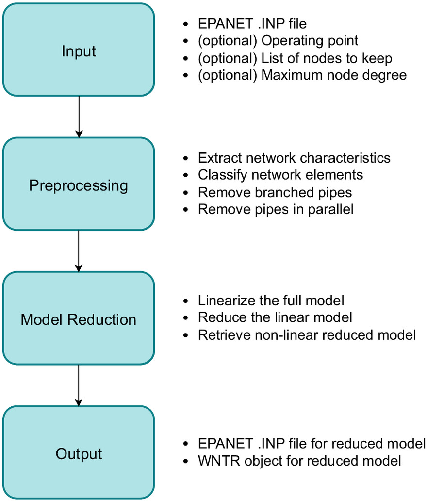
MAGNets employs the variable elimination reduction method to remove nodes and links from a water network model while retaining control elements and elements that are of interest to the user (Ulanicki et al. 1996). Users are able to run simulations of a water network that can be significantly smaller in size than the original network, thus considerably reducing run time. MAGNets functionality is briefly described below, and Fig. 1 summarizes the main modeling framework.
Package Overview
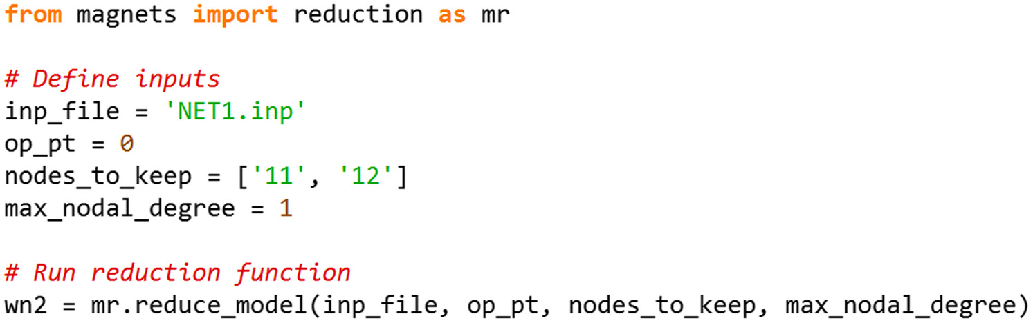
MAGNets offers the function reduce_model that allows the user to submit a water network model and customize the model by choosing: (1) a specific operating point (around which the model will be linearized); (2) a list of nodes that should remain in the reduced model; and (3) a maximum nodal degree value for the nodes removed from the model. Fig. 2 demonstrates the reduce_model function with the following inputs: (1) the inp_file is a .INP file containing the water network model object; (2) the op_pt is the operating point, which represents a multiple of the reporting time step. If the user does not provide an operating point, it will be set by default to 0, i.e., the start time of the simulation. Users are encouraged to check if the reporting time step of the .INP file aligns with the simulation period they are interested in investigating and then adjusting accordingly; (3) nodes_to_keep is a list of nodes to keep in the model. If the user does not provide a list of nodes to be retained in the model, every node that is not a special element or that is not connected to a special element will be removed from the model (as will be described below); and (4) max_nodal_degree, which dictates the maximum nodal degree of nodes being removed from the model. The nodal degree of a node is equal to the number of pipes incident to the node. For example, if max_nodal_degree = 1, all nodes that are not in nodes_to_keep and that are connected to only one other node by one pipe will be iteratively removed from the model. The reduce_model function returns two outputs: (1) a .INP of the reduced network model that will be created in the destination folder of the original model, and (2) a water network model object representing the reduced network model (shown as wn2 in Fig. 2) that the user can access using the USEPA WNTR Python package (Klise et al. 2017) without having to import the new .INP file.
Preprocessing
Prior to executing the main model reduction algorithm, MAGNets performs several preprocessing steps. First, the .INP file provided by the user is converted into a water network model object that is compatible with WNTR. Basic characteristics of the network are extracted and stored and are used as the basis to determine which nodes will be removed from the model. Nodes are classified as special, non-removable, or removable, and including a node in subsequent calculations is dependent of this initial categorization. Special nodes include reservoirs, tanks, source nodes, and junctions that have been assigned control rules. Special links include pumps, valves, and links that have been assigned control rules. Non-removable nodes include nodes that are directly connected to special nodes or special links. If the user provides a list of nodes to keep in the model, all nodes in that list are assigned non-removable status. All nodes in the model that are not assigned special or non-removable status are categorized as removable and will be removed during the model reduction process. Second, before the aggregation and reduction process is executed, the model is trimmed by removing branches and parallel pipes in order to enhance the efficiency of the reduction process. Every dead-end node connected by a single pipe is removed from the model and the demand attributed to that node is allocated to the upstream node. Several iterations are performed until all dead-end nodes and branched pipes are removed from the model. After branched pipes are removed from the model, all parallel pipes are identified and replaced by a single equivalent pipe (Boulos et al. 2006).
Model Reduction
The main steps of the model reduction procedure are: (1) non-linear equations describing the hydraulics of the system are constructed and linearized around the operating point; (2) the linearized system of equations is reduced through the method of Gaussian elimination, resulting in the redistribution of nodal demands, the creation of new fictitious links, and the deletion of unnecessary nodes from the model; and (3) the updated linearized equations are converted back into non-linear form to derive the characteristics of the reduced water network model, which is subsequently returned to the user. The reduction process is briefly described below and the full details of the process can be found in Ulanicki et al. (1996) and Alzamora et al. (2014).
Step 1: Compute linear conductances
After the model has been trimmed, all non-special pipes are assigned conductance values that retain the diameter, length, and roughness of the pipes. The head loss equation for a single pipe with diameter , length , and roughness coefficient can be formulated aswhere is the flow rate in the pipe connecting nodes and , , , and , and is the Hazen-Williams unit constant (Boulos et al. 2006). To reduce rounding errors, the value of is calculated as the mean value of the unit coefficients for each pipe in the network based on the values extracted from simulation results using the equation , where is the head loss at the operating point. Rearranging Eq. (1), we getwhere and .
(1)
(2)
Linearizing Eq. (2) around an operating point, we getwhere is linearized pipe conductance. Additionally, for each node , the total linearized conductance is computed as the sum of all linear conductances of the incident pipes aswhere pipe belongs to the set of all pipes incident to node .
(3)
(4)
Step 2: Reduce the linear model
After all conductance values are linearized, the list of nodes to be removed is sorted in ascending order based on the node degree. The node with the lowest node degree is deemed the “removal node” and all nodes connected to the removal node are labeled “adjacent nodes”. For each node that is being removed, two actions occur: (1) Nodal demand of node is allocated to its adjacent nodes proportional to the linear conductance, and the new demand of each adjacent node is updated aswhere and are the base demands at nodes and , respectively, and is the new adjusted base demand at node . (2) The linear conductances of pipes connecting all the adjacent nodes will be updated as follows:
(5)
(6)
If two adjacent nodes were not previously connected, then and a new fictitious pipe is created. The code optimizes the order in which the nodes are removed from the model to minimize the number of fictitious pipes that are added to the model. After all adjacent nodes and connected links are updated, node and all the incident pipes are removed from the model, and the list of nodes and pipes remaining in the model is updated and again sorted in ascending order based on node degree, with the “removal node” for the next iteration being the new node with the lowest node degree. The process repeats in an iterative manner until all nodes in the list of nodes to be removed are removed from the model.
Step 3: Retrieve properties of the reduced non-linear model
At the final stage, the non-linear properties of the reduced model, i.e., aggregated demands and pipe properties, are retrieved from the linearized conductance as follows:
(7)
We assume that all new fictitious pipes have roughness coefficient and length equals to the average length of all pipes in the original model, which can be substituted into Eq. (7) to calculate the new diameter of each link. Notably, the new pipe diameters, which are calculated according to the pipe conductances, are not expected to be reasonable values on par with the original model. The final outcome is a new hydraulic model with a compatible .INP file that can be used to simulate network hydraulics in EPANET or WNTR.
Summary of Modeling Assumptions
The following assumptions were made when developing the package: (1) Reservoirs, tanks, and junctions with control rules as well as pumps, valves, and links with control rules are classified as special elements and will not be removed from the model; (2) Any junction with a negative base demand value will not be removed from the model; and (3) MAGNets is best suited to reduce models of systems in which demand nodes follow the same demand pattern. Hence, if junctions have varying demand patterns attributed to them, we recommended homogenizing the demand pattern of all non-special nodes before performing model reduction in order to optimize the results and minimize deviations of the reduced model from the original model. However, model reduction can still be partially applied when demand nodes follow different demand patterns. Preis et al. (2011) suggested grouping nodes based on a spatial analysis and assigning each group a unique demand pattern, assuming that consumers within the same area of the system will exhibit similar characteristics. Alzamora et al. (2014) provided additional recommendations for handling nodes with different demand patterns. We provide an example application for the network with multiple demand patterns in the “Results” section.
Results
Next, we evaluated the performance of MAGNets by examining: (1) accuracy and running times using 12 networks of varying complexity, (2) selection of the operating point, (3) comparison of different orders of node removal, (4) comparison with WNTR skeletonization, and (5) application to a network with mulitple demand patterns.
Package Performance
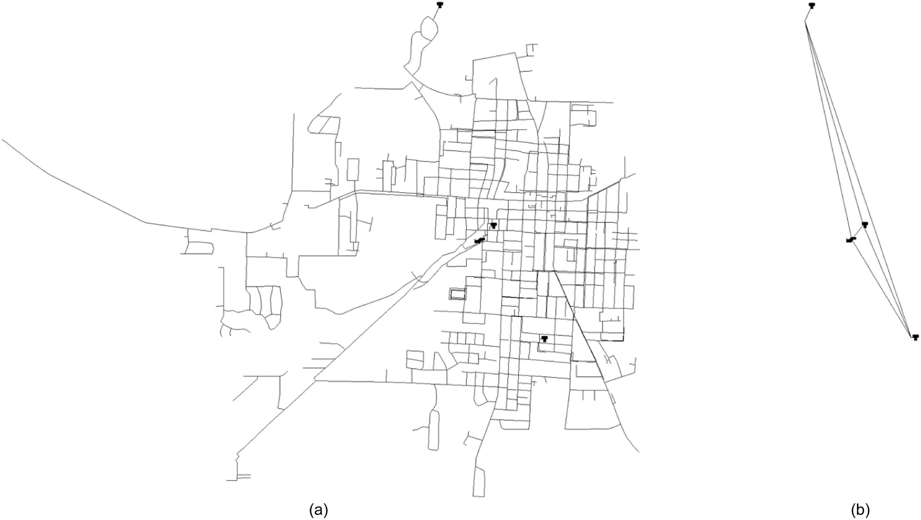
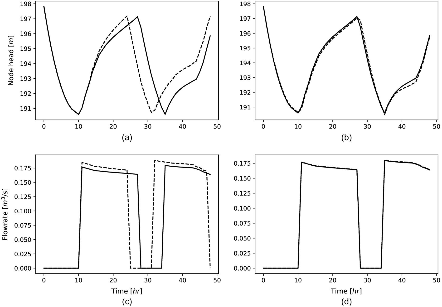
The performance of the package was tested using 12 networks of varying complexity obtained from Rossman et al. (2020), Hernandez et al. (2016), and Ostfeld and Salomons (2008). Table 1 summarizes the tested networks, number of nodes in the original and reduced models, running times, and the maximum error. The MAGNets repository (Thomas and Sela 2022) contains all the tested networks and several example codes that demonstrate the functionality of the package. The networks were modified prior to reduction to ensure that all nodes to be removed had the same demand pattern. The error was computed as the maximum relative error (%) during the entire duration of the simulation among all remaining nodes in the reduced model, where the relative error was computed as the difference in nodal heads in the reduced and original models divided by the nodal head in the original model. Results demonstrate that the reduction process running times for all networks were under 3.3 s with the exception of BWSN2, which took approximately 4 min. Additionally, the maximum observed errors in all networks were under 5.5%. As an example, Fig. 3 shows the full and reduced network topology for KY2, and Fig. 4 shows the flow rate and head at a selected pump and tank. The codes to reproduce Table 1 and Figs. 3 and 4 are available on GitHub Repository https://github.com/meghnathomas/MAGNets/tree/master/publications.
| Network | Number of junctions in original model | Number of junctions in reduced model | Reduction time (s) | Maximum error (%) |
|---|---|---|---|---|
| NET1 | 9 | 2 | 0.03 | 0.12 |
| NET2 | 35 | 3 | 0.05 | 0.55 |
| NET3 | 92 | 7 | 0.08 | 3.49 |
| KY1 | 791 | 19 | 1.03 | 0.48 |
| KY2 | 811 | 5 | 3.29 | 0.56 |
| KY3 | 269 | 14 | 0.28 | 0.06 |
| KY4 | 959 | 9 | 1.32 | 1.20 |
| KY5 | 420 | 21 | 0.44 | 2.60 |
| KY6 | 543 | 9 | 0.60 | 0.08 |
| KY7 | 481 | 6 | 0.57 | 0.09 |
| KY8 | 1,325 | 14 | 3.10 | 0.25 |
| BWSN2 | 12,523 | 20 | 232.82 | 5.50 |
Selection of Operating Point
For most networks, the deviation of heads in the reduced model from those of the original model can be attributed to slight temporal misalignment in control rules activation causing changes in tank filling times. An example of this can be demonstrated by running the MAGNets reduce_model function on network KY2 and comparing the heads of tank T-2 in the original and reduced models. The control rules operating on the tanks in the network dictate that each tank will be opened and closed at specific pressure values. As the network has been linearized around a specific operating point, slight changes in heads at other times along the simulation duration are to be expected. However, these slight changes then affect the time step in which the tank achieves the head that will result in it opening or closing. Fig. 4 demonstrates how the choice of operating point can affect the reduced model accuracy: if operating point 0 is chosen for network KY2 [as is shown in Figs. 4(a and c)], the hydraulic performance of the reduced model begins to deviate from the original model as the tank head begins to drop earlier than in the original model, thus causing a temporal shift in the head values at tank T-2. This difference in tank head is mirrored in the flow rate of Pump-1. Errors in pressure heads along the rest of the time duration remain within reasonable limits. Upon testing and calculating the error for all possible operating points, it could be determined that operating point 13 produced very similar simulation results for the original and reduced models, as can be seen in Figs. 4(b and d).
Errors in heads and flows between original and reduced network models can be minimized by testing a wide range of operating points and using different reduced models for specific operating conditions. It is also possible to reduce errors by leaving more nodes in the reduced model; however, this requires careful consideration. Users may also employ the max_nodal_degree input to control the level of reduction, e.g., trim only branches and merge pipes connected in series. Another strategy to only partially reduce the model is to halt the reduction process after a desired fraction of nodes in the original model have been removed. Figs. S1 and S2 show the median error, reduction time, and number of pipes in the reduced models for KY2 when controlling the maximum degree of the nodes removed (i.e., 1, 2, 3, and no restriction) and controlling the number of removed nodes (25%, 50%, and 75%), respectively.
Comparison of Different Node Removal Orders
We investigated the impact of the order in which the nodes are removed on the accuracy and running times of model reduction. Upon determining the list of nodes that can be removed from the model, the list was reordered in three ways: randomly, statically, and dynamically, each time removing 25%, 50%, 75%, and 100% of removable nodes. The results of the random ordering are the mean results of ten different randomized ordered lists. The statically ordered list was determined by arranging the list of nodes to be removed in ascending order of node degree at the beginning of the reduction process. In the dynamically ordered list, the nodes are removed in ascending order by the node degree, which is constantly updated each time a node is removed from the network.
We defined three performance criteria: (1) the accuracy of the reduced model, which was computed as the median relative error between the pressure heads of nodes remaining in the reduced network and the equivalent nodes in the original network; (2) model reduction time; and (3) number of links remaining in the reduced model. We show results for three networks of increasing size, NET3 (92 nodes), KY1 (791 nodes), and BWSN2 (12,523 nodes). Fig. 5 shows the three performance criteria under different removal sequences and node list partitions (25%, 50%, and 75%) for the test networks. Each row represents a performance criterion and each column represents a network. For example, the figure on the top left shows the median percentage error between the original NET3 model and reduced models of NET3 when 25%, 50%, and 75% of the nodes are removed in static, random, and dynamic order. The figure in the middle left demonstrates the reduction time in seconds, and the bottom left figure shows the number of pipes left in the reduced model for NET3 under the same criteria. Overall, the dynamically ordered lists outperformed the other orders in all three metrics of interest, resulting in lower median error, significantly fewer pipes retained in the reduced model, and a lower reduction time, with the exception of greater reduction time for the small network NET3. Results for NET3 differ from those of KY1 and BWSN2 most likely because the network was considerably smaller in size and the time required for reordering the nodes in each iteration exceeded that of removing the elements; however, the reduction times for all ordering methods and list sections were very similar. Surprisingly, the statically ordered list performed the worst in all three performance criteria. Statically ordered reduction created more pipes in the model for all three networks, thus significantly affecting running times because the number of elements in the model increased with each iteration. Statically ordered removal also generated high median errors, on par with or surpassing that of the random ordered removal. Additionally, the results revealed that error does not necessarily correlate with the size of the network or with the number of nodes left in the model. The statically ordered removal of 75% of nodes for BWSN2 had a running time of more than 72 hours, so those results were not included in the analysis.
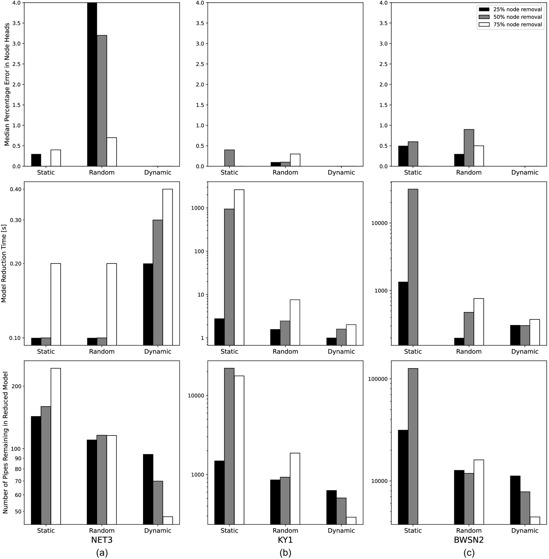
We can conclude that dynamically ordering the nodes to be removed best serves the purpose of maximizing model accuracy and minimizing reduction time and model complexity. Randomly ordered lists would be the next best alternative with lower reduction times and model complexities compared to statically ordered lists while maintaining a comparable level of accuracy. Following these results, dynamic ordering of nodes was implemented in MAGNets.
Comparison with WNTR Skeletonization
In this section, we compare the proposed approach with the WNTR skeletonization function. WNTR is an open-source Python package that offers a skeletonization functionality, which allows the user to remove branches and merge pipes in series and in parallel (Klise et al. 2017). WNTR skeletonization function requires the user to provide a network .INP file and a threshold for maximum pipe diameter for pipe removal, where pipes with diameters less than the threshold will be removed from the model. When pipes are removed/merged, the demands of the incident nodes that are removed are assigned to the closest neighboring node by appending the base demand value and demand pattern of the removed node as a new demand category for the receiving neighbor node. Then, the properties of the new equivalent pipe are updated based on the characteristics (length, diameter, roughness) of the removed pipes. However, WNTR does not allow the user to control which nodes to keep in the model or remove nodes with nodal degree greater than 2. In contrast, MAGNets reallocates the base demands of nodes that are removed from the model to its adjacent nodes proportionally to the conductances of the incident pipes, enables the user to specify which nodes should remain in the model, and allows for the removal of nodes with a nodal degree greater than 2.
We demonstrate the comparison of the performance of WNTR and MAGNets using network KY2 by removing nodes with degrees 1 and 2. For WNTR, the largest pipe diameter in the network was supplied as the diameter threshold. For MAGNets, an operating point of 13 hours was provided as an input. The original KY2 model contained 811 nodes (see Table 1 and Fig. 3). Removing only branches from the KY2 model resulted in a model with 593 nodes (a 27% reduction) and yielded identical reduced models with WNTR and MAGNets, in which the absolute relative error between nodal heads in the reduced and original models was lower than for all nodes. Removing additional nodes with degree 2 resulted in a reduced model with 459 nodes (a 43% reduction) for both WNTR and MAGNets. Although the size of the reduced models is the same, model properties are different since different methods are applied in the reduction process. Fig. S3 shows the absolute relative error for the reduced models resulting in removing nodes with degrees 1 and 2 using MAGNets (top left) and WNTR (top right). The shaded areas represent the 75%, 95%, and 100% percentiles, and the red line represents the mean absolute error. We observe that both reduced models exhibit a very good match with the original models in terms of the errors, where MAGNets slightly outperforms WNTR with a maximum error of 0.07% compared to 0.14%. However, as demonstrated earlier, MAGNets is capable of reducing the model even further. Using the reduce_model function without limiting the node degree of the removed nodes, the model size is reduced to only five nodes (a 99% reduction) (Fig. 3) and the largest absolute relative error for the heads of the remaining nodes is 0.56% (Table 1). Fig. S3 (bottom) shows the distribution of error for all nodes throughout the simulation duration, where shaded areas represent the 75%, 95%, and 100% percentiles, and the red line represents the mean absolute error.
Models with Multiple Demand Patterns
A set of scenarios for the C-Town network was evaluated to test the capabilities of MAGNets’ reduce_model function when it is confronted with different demand patterns and when the user wishes to reduce specific sections of the network. The C-Town network model contains five different District Metered Areas (DMAs), each with a unique demand pattern (Ostfeld et al. 2012). In order to adapt the reduction strategy to C-Town, a list of boundary nodes that lay on the borders of DMAs was provided as the nodes_to_keep input for each call of the reduce_model function. A stage-wise reduction of the C-Town model was performed by first removing all nodes with nodal degree 1 from the model and then removing nodes with nodal degree 2 from DMA1, DMA3, and DMA5. The number of nodes in the final reduced model decreased from 388 to 176 (a 55% reduction). Fig. S4 shows the network layout of the full and reduced models. The time series of the relative error of the heads at each node reveals that even at this high level of reduction the reduced model performs very similarly to the original model (see Fig. S5 ). The relative errors are negligible for the majority of the extended period simulation with the exception of a few large spikes which can be attributed to time step delays in control rules activation. For example, Fig. S6 shows that spike 1 and spike 2 in Fig. S5 can be explained by delays in the operational status of pump PU2 based on the water level of tank T1. The maximum difference between heads of nodes in the original and reduced models ranges from to , while the mean difference ranges from to . Fig. S7 shows the distribution of errors and demonstrates that the mean absolute relative percentage error is 0.06% or lower for all nodes remaining in the reduced model. Finally, Fig. S8 shows the spatial distribution of the errors, demonstrating that nodes with similar error are located close together in the reduced C-Town model, and the nodes with the largest errors after reduction lie in DMA1 or are adjacent to pumps. These examples show that, if applied carefully, MAGNets can also be used to significantly reduce models with varying demand patterns. Users are advised to attempt a range of reduction strategies in order to maximize the usefulness and accuracy of the reduced models.
Conclusions
This paper introduces MAGNets, an open-source Python package for model reduction of water networks based on variable elimination method. Users may employ the package to reduce a network around a specific operating point and are able to customize which nodes to retain in the reduced model or control the maximum nodal degree of the removed nodes. MAGNets is a tool that may be utilized by researchers and practitioners to reduce the size of networks for problems such as state estimation, optimal operation, and designing control rules. MAGNets has the potential of further development through the addition of error analysis functions that will allow the user to tailor the allowable deviation of the reduced model from the original model to their requirements by choosing better operating points or by leaving more nodes in the reduced model. Further extension should also include aggregation of nodes with multiple demand patterns. To promote research reproducibility and usability, all source codes, software documentation, and examples are provided with the package. The most up-to-date version of MAGNets can be accessed at the GitHub Repository: https://github.com/meghnathomas/MAGNets.
Supplemental Materials
File (supplemental materials_jwrmd5.wreng-5486_thomas.pdf)
- Download
- 811.98 KB
Data Availability Statement
All data, models, and code generated or used throughout the study are available at Thomas and Sela (2022).
Reproducible Results
Lu Xing, Helena Tiedmann, and Matthew Frankel (University of Texas at Austin), downloaded, installed, and ran the model using the input data sets and reproduced the results in Table 1.
Acknowledgments
This work was supported by the National Science Foundation under Grant 1943428.
References
Alzamora, F. M., B. Ulanicki, and E. Salomons. 2014. “Fast and practical method for model reduction of large-scale water-distribution networks.” J. Water Resour. Plann. Manage. 140 (4): 444–456. https://doi.org/10.1061/(ASCE)WR.1943-5452.0000333.
Anderson, E. J., and K. H. Al-Jamal. 1995. “Hydraulic-network simplification.” J. Water Resour. Plann. Manage. 121 (3): 235–240. https://doi.org/10.1061/(ASCE)0733-9496(1995)121:3(235).
Boulos, P. F., K. E. Lansey, and B. W. Karney. 2006. Comprehensive water distribution systems analysis handbook for engineers and planners. Broomfield, CO: MWH Soft, Inc.
Broad, D. R., H. R. Maier, and G. C. Dandy. 2010. “Optimal operation of complex water distribution systems using metamodels.” J. Water Resour. Plann. Manage. 136 (4): 433–443. https://doi.org/10.1061/(ASCE)WR.1943-5452.0000052.
Deuerlein, J. W. 2008. “Decomposition model of a general water supply network graph.” J. Hydraul. Eng. 134 (6): 822–832. https://doi.org/10.1061/(ASCE)0733-9429(2008)134:6(822).
Hamberg, D., and U. Shamir. 1988. “Schematic models for distribution systems design. I: Combination concept.” J. Water Resour. Plann. Manage. 114 (2): 129–140. https://doi.org/10.1061/(ASCE)0733-9496(1988)114:2(129).
Hernandez, E., S. Hoagland, and L. E. Ormsbee. 2016. WDSRD: A database for research applications. Lexington, KY: Univ. of Kentucky.
Klise, K. A., M. Bynum, D. Moriarty, and R. Murray. 2017. “A software framework for assessing the resilience of drinking water systems to disasters with an example earthquake case study.” Environ. Modell. Software 95 (4): 420–431. https://doi.org/10.1016/j.envsoft.2017.06.022.
Krieg, H., D. Nowak, and M. Bortz. 2018. “Surrogate models for the simulation of complex water supply networks.” In Proc., WDSA/CCWI Joint Conf. Kingston, ON, Canada: Queen’s Univ.
Kumar, S. M., S. Narasimhan, and S. M. Bhallamudi. 2008. “State estimation in water distribution networks using graph-theoretic reduction strategy.” J. Water Resour. Plann. Manage. 134 (5): 395–403. https://doi.org/10.1061/(ASCE)0733-9496(2008)134:5(395).
Maschler, T., and D. A. Savic. 1999. “Simplification of water supply network models through linearization.” Ph.D. thesis, School of Engineering, Univ. of Exeter.
Moser, G., S. G. Paal, and I. F. Smith. 2015. “Performance comparison of reduced models for leak detection in water distribution networks.” Adv. Eng. Inf. 29 (3): 714–726. https://doi.org/10.1016/j.aei.2015.07.003.
Ostfeld, A., et al. 2012. “Battle of the water calibration networks.” J. Water Resour. Plann. Manage. 138 (5): 523–532. https://doi.org/10.1061/(ASCE)WR.1943-5452.0000191.
Ostfeld, A., and E. Salomons. 2008. “Sensor network design proposal for the battle of the water sensor networks (BWSN).” In Proc., Water Distribution Systems Analysis Symp. 2006. Reston, VA: ASCE.
Perelman, L., M. L. Maslia, A. Ostfeld, and J. B. Sautner. 2008. “Using aggregation/skeletonization network models for water quality simulations in epidemiologic studies.” J. Am. Water Works Assn. 100 (6): 122–133. https://doi.org/10.1002/j.1551-8833.2008.tb09659.x.
Preis, A. J., A. J. Whittle, A. J. Ostfeld, and L. J. Perelman. 2011. “Efficient hydraulic state estimation technique using reduced models of urban water networks.” J. Water Resour. Plann. Manage. 137 (4): 343–351. https://doi.org/10.1061/(ASCE)WR.1943-5452.0000113.
Rossman, L., H. Woo, M. Tryby, F. Shang, R. Janke, and T. Haxton. 2020. Epanet 2.2 user manual. Washington, DC: US Environmental Protection Agency.
Saldarriaga, J. G., S. Ochoa, D. Rodriguez, and J. Arbeláez. 2009. “Water distribution network skeletonization using the resilience concept.” In Proc., Water Distribution Systems Analysis 2008. Reston, VA: ASCE.
Shamir, U., and E. Salomons. 2008. “Optimal real-time operation of urban water distribution systems using reduced models.” J. Water Resour. Plann. Manage. 134 (2): 181–185. https://doi.org/10.1061/(ASCE)0733-9496(2008)134:2(181).
Thomas, M., and L. Sela. 2022. MAGNets. Austin, TX: Texas Data Repository. https://doi.org/10.18738/T8/P4MCQV.
Ulanicki, B., A. Zehnpfund, and F. Martinez. 1996. “Simplification of water distribution network models.” In Proc., 2nd Int. Conf. on Hydroinformatics, 493–500. Zurich, Switzerland: International Water Association.
Wang, S., A. F. Taha, A. Chakrabarty, L. Sela, and A. A. Abokifa. 2022. “Model order reduction for water quality dynamics.” Water Resour. Res. 58 (4): e2021WR029856. https://doi.org/10.1029/2021WR029856.
Information & Authors
Information
Published In

Journal of Water Resources Planning and Management
Volume 149 • Issue 2 • February 2023
Copyright
This work is made available under the terms of the Creative Commons Attribution 4.0 International license, https://creativecommons.org/licenses/by/4.0/.
History
Received: Jul 20, 2021
Accepted: Nov 1, 2022
Published online: Dec 14, 2022
Published in print: Feb 1, 2023
Discussion open until: May 14, 2023
ASCE Technical Topics:
- Computer models
- Continuum mechanics
- Dynamics (solid mechanics)
- Engineering fundamentals
- Engineering mechanics
- Forces (type)
- Hydraulic engineering
- Hydraulic models
- Hydraulic networks
- Hydraulic structures
- Magnetic fields
- Model accuracy
- Models (by type)
- Optimization models
- Simulation models
- Solid mechanics
- Water and water resources
- Water management
- Water supply
- Water supply systems
Authors
Metrics & Citations
Metrics
Citations
Download citation
If you have the appropriate software installed, you can download article citation data to the citation manager of your choice. Simply select your manager software from the list below and click Download.
Cited by
- James H. Stagge, David E. Rosenberg, Anthony M. Castronova, Avi Ostfeld, Amber Spackman Jones, Journal of Water Resources Planning and Management’s Reproducibility Review Program: Accomplishments, Lessons, and Next Steps, Journal of Water Resources Planning and Management, 10.1061/JWRMD5.WRENG-6559, 150, 8, (2024).
- Meghna Thomas, Lina Sela, A Mixed‐Integer Linear Programming Framework for Optimization of Water Network Operations Problems, Water Resources Research, 10.1029/2023WR034526, 60, 2, (2024).