Hydrodynamic Mechanisms and Pathways of Potential Navigation Channel Shoaling by Nearby Parallel Islands

Holzenthal, Elizabeth R.; Bain, Rachel L.; Krafft, Douglas R.; Cadigan, Jack A.; Styles, Richard

doi:10.1061/JWPED5.WWENG-2127

Open access

Technical Papers

Sep 17, 2024

Hydrodynamic Mechanisms and Pathways of Potential Navigation Channel Shoaling by Nearby Parallel Islands

Authors: Elizabeth R. Holzenthal, Ph.D. https://orcid.org/0000-0002-6211-4113 [email protected], Rachel L. Bain, Ph.D. [email protected], Douglas R. Krafft https://orcid.org/0000-0002-8922-6000 [email protected], Jack A. Cadigan, Ph.D. [email protected], and Richard Styles, Ph.D. [email protected]Author Affiliations

Publication: Journal of Waterway, Port, Coastal, and Ocean Engineering

Volume 151, Issue 1

https://doi.org/10.1061/JWPED5.WWENG-2127

PDF

Abstract

As the demand for transcontinental commerce has increased over the past century, navigation channels have been maintained at increasingly greater depths to continue access of deep draft vessels to inland ports. Over time, these deep navigation channels require routine dredging to counteract the gradual processes of sedimentary accumulation, known as shoaling, that can enter the channel from terrestrial or oceanic sources through natural (e.g., tides, streamflow, runoff) or anthropogenic (e.g., vessel wake) processes. To limit the cost of moving the dredged material to upland or offshore storage facilities and to prevent long-term sediment loss from the system, the material can instead be reused locally to build marsh or island habitats. While the various environmental impacts of keeping and reusing the material within the sourcing embayment have been investigated at length, the hydrodynamic impacts of large-scale within-embayment placements have previously been understudied, particularly regarding potential changes to navigation channel shoaling. In this work, we use numerical models to investigate how channel-parallel linear island features may modify sediment transport mechanisms and pathways, and discuss long-term shoaling implications. Based on the various tested channel and embayment geometries, taken from nautical charts detailing the evolving topobathymetric history of Lake Calcasieu and the Calcasieu Shipping Channel (Louisiana, USA), linear and near-continuous islands are shown to have the potential to increase sedimentation in the channel by altering both local hydrodynamics around the islands and estuarine-scale tidal dynamics. However, the degree to which the islands are continuous (i.e., number and size of gaps between islands) and the dominant forcing factors (i.e., tidally driven versus wind-driven circulation) are shown to limit the increase in shoaling likelihood by island presence.

Introduction

Centuries of navigation channel deepening across the globe have led to various strategies for using, storing, or disposing of the resulting dredged sediment. In the United States, the federal standard for dredged material management requires the U.S. Army Corps of Engineers (USACE) to select the least-cost disposal alternative which meets environmental standards and is consistent with sound engineering practices (EPA and USACE 2007). Consequently, dredged sediment has historically been disposed offshore in ocean dredged material disposal sites or stored in upland confined disposal facilities. Alternatively, repurposing the sediment dredged from channel bottoms presents an opportunity for environmental and economic benefits as compared to long-term disposal. For example, dredged material can be used to offset anthropogenic land loss and sea level rise by creating wetland and intertidal habitats or nourishing eroding beaches. Renewed emphasis on the beneficial use of dredged material (BUDM) has resulted in increasing quantities of sediment being retained within embayed coastal systems for restoration purposes. However, due to the dynamic interactions of variable physical drivers (e.g., wind, wave, tide), BUDM properties (e.g., sediment characteristics, placement volume, shape), and other factors (e.g., ship wake, basin morphology, aquatic flora and fauna), there is limited generalized understanding of how sediment placement within an embayment may influence system-scale sediment transport and its pathways, particularly regarding unintended consequences to navigation maintenance requirements (Krafft et al. 2022). USACE’s current goal of achieving 70% BUDM by the year 2030 (Spellmon 2023) underscores the importance of fully understanding the long-term effects that different BUDM strategies have on coastal systems.

Although a wide body of literature exists on the hydrodynamic impacts of deepening, such works are not necessarily linked to regional sediment management practices. Analytical derivations indicate that deepening navigation channels reduces tidal damping (Friedrichs and Madsen 1992; Winterwerp and Wang 2013), and tidal amplification by deepening has been evidenced in estuaries across the globe (Amin 1983; Cai et al. 2012; Winterwerp et al. 2013; Vellinga et al. 2014; de Jonge et al. 2014; Ralston et al. 2019; Eidam et al. 2020). The combination of greater depth and/or larger tidal range may enhance salinity intrusion and estuarine stratification (de Jonge et al. 2014), both of which promote fine sediment flocculation and accelerated shoaling rates, which is the rate at which sediment accumulates in the channel. The re-entry of dredged sediment has been considered by practitioners as a possible contribution to channel shoaling rates, particularly when material is placed just outside the navigation channel, such as by the historical practice of “side-casting” (Mathewson and McHam 1977; Drapeau 1988; Hayter et al. 2012; Byrnes et al. 2013; Lambert et al. 2013; Bever et al. 2014; Lackey et al. 2020). However, previous works directly quantifying the impact of in-bay dredged sediment placement have emphasized environmental considerations rather than hydrogeomorphic ones, including its effect on vegetation (Fehring et al. 1979; McVay et al. 1980; Bolam and Rees 2003; Goldberg and Rillstone 2012; De Vet et al. 2020; Sullivan et al. 2022), fauna (Stieglitz and Wilson 1968; Landin and Engler 1986; Scarton et al. 2013; Wnek et al. 2013; Krainyk et al. 2020; Chapman et al. 2019; Gamblin et al. 2023), and soil and water quality (Slotta et al. 1973; Sisson et al. 2010).

Previous works specifically investigating changes in hydrogeomorphic conditions resulting from in-bay placement are often constrained to the local scale (Christiansen and Hodges 2016; Fleri et al. 2019), but a few notable exceptions with a more holistic scope have shown that hydrodynamic feedback at the scale the deposited sediment can trigger changes in system-scale behavior, such as by altering regional hypsometry (Eidam et al. 2020), tidal prism (Liria et al. 2009), and the flow-carrying cross section (Berkowitz et al. 2021). Direct observations by Vogel and Kana (1985) found that following the placement of 1.53 million cubic meters (Mm³) of dredged sediment on the flood tidal delta, Moriches Inlet (New York, USA) switched from a flood-dominant system to ebb-dominant, leading to a net export of sediment from the back-barrier region. Goodwin (1987) modeled system-scale alterations to residual circulation in Tampa Bay before and after dredged material placement, noting an increase in flushing between 1880 and 1972. More recently, Stark et al. (2017) modeled marsh construction via sediment placement along the channel banks in the Western Scheldt Estuary. Their results indicated that constructing tidal flats at or above the mean water level in the center of the channel would enhance ebb dominance, whereas constructing tidal flats near low water would enhance flood dominance, with the effect on tidal behavior extending as far as 15 kilometers (km) away from the placement site. van Dijk et al. (2021) likewise modeled alternative placement strategies for the Western Scheldt Estuary to identify placement options that would result in the lowest cumulative dredging requirements over a 40-year horizon. While these recent works represent encouraging progress toward a systematic understanding of best practices for in-estuary dredged material placement, coastal engineering guidance on effective placement strategies for a variety of inlet and embayment morphologies is still lacking. In this work, we use numerical models to investigate changes to shoaling potential by the formation of islands alongside a deep-draft navigation channel within an otherwise shallow open-water embayment on the Gulf Coast of the United States. We use a month-long numerical simulation to identify sections of the navigation channel most susceptible to shoaling and use a particle tracking model to investigate possible sediment pathways between the BUDM islands and the channel.

Background

To quantify the hydrodynamic impacts and geomorphic implications of channel-adjacent BUDM islands, we use the topobathymetric history of Lake Calcasieu, located in southwestern Louisiana (LA) (Fig. 1) rather than developing a computational mesh of an idealized embayment–island system. The Lake Calcasieu and Calcasieu River system provide an ideal setting for this study not only because the Calcasieu Shipping Channel (CSC) is flanked by kilometer-scale linear islands constructed from dredged material, but because dredging operations and resulting changes in bathymetry are well documented by the USACE Chief of Engineers’ Annual Reports and nautical charts by the National Ocean Service (NOS) of the National Oceanic and Atmospheric Administration (NOAA) and the United States Coast and Geodetic Survey (USCGS), now known as NOAA’s National Geodetic Survey (NGS).

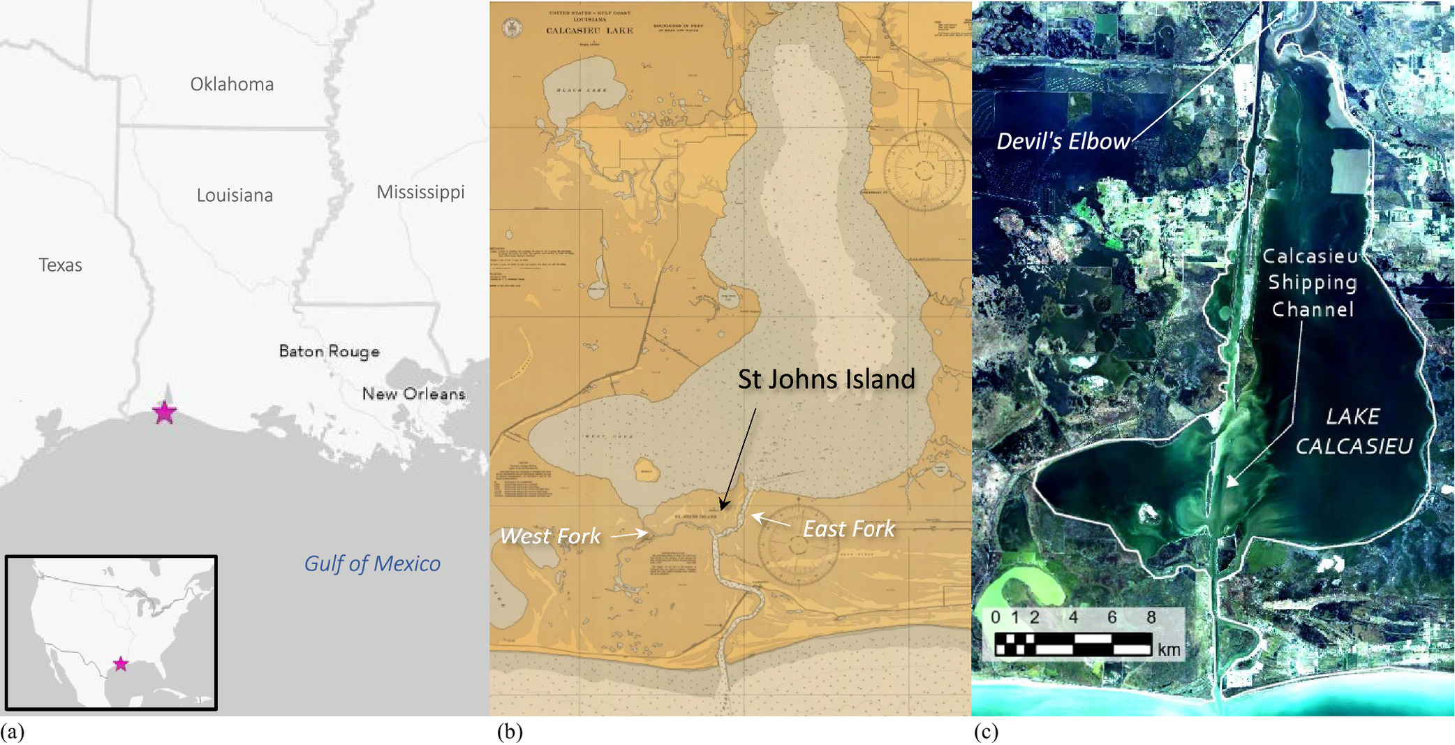
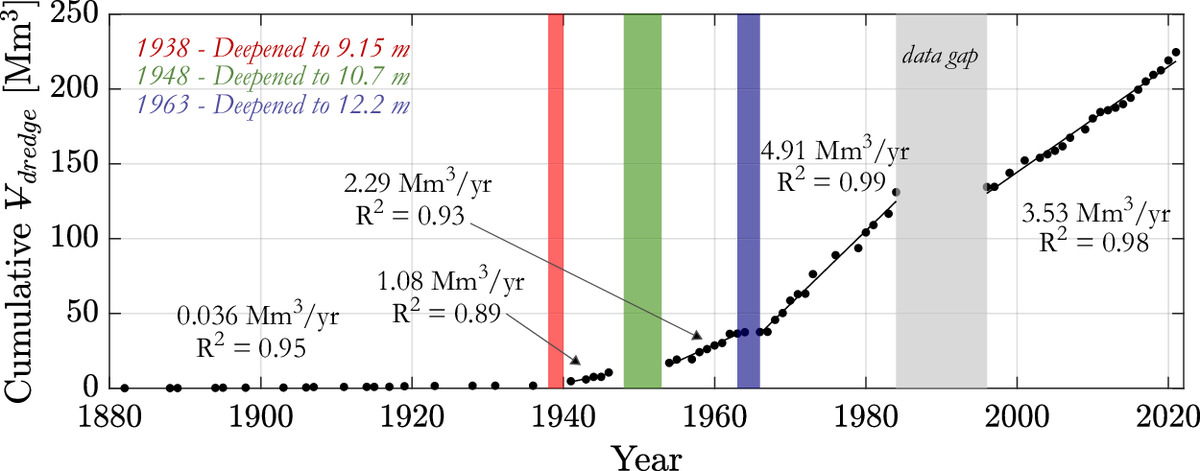
Fig. 1. (a) Location of the study site (star) in relation to the southeastern United States and the Gulf of Mexico (base map © ESRI 2024); (b) aerial view of Lake Calcasieu as depicted in 1935 nautical chart (map from Coast and Survey 1935), as well as (c) modern satellite imagery (image © NAIP 2022).

Anthropogenic modification of the lake and channel hypsometry began in 1873 following the decision of USACE to deepen the submerged bar at the head of Calcasieu Pass at its outlet to the Gulf of Mexico to ensure commercial vessel entry to Lake Charles at mean low tide (USACE Chief’s Reports). In 1938, a cutoff was constructed across the original serpentine outlet, [Figs. 1(b and c)], and a 9.15-meter (m), or 30-foot (ft), deep-draft linear channel was developed between the Gulf of Mexico and the top of Lake Calcasieu near Deatonville, LA. The channel has been deepened twice since then, once in 1948 to 10.7 m (35 ft) and again in 1963 to 12.2 m (40 ft), and material removed from the channel during these deepening events was side-cast to form the linear islands that still exist today. Data from the Chief of Engineers’ Annual Report suggest that each major deepening event coincides with an increase in the maintenance dredging rate, from 0.036 Mm³/yr pre-channelization, to 1.08 Mm³/yr following channelization and deepening to 9.15 m, to 2.29 Mm³/yr following deepening to 10.7 m, to 4.91 Mm³/yr following deepening to 12.2 m (Fig. 2). This co-occurrence of navigation channel deepening, channel-adjacent island formation, and increased shoaling rates makes the historical evolution of the Calcasieu system a prime candidate for the investigation into the potential impacts of large-scale topobathymetric changes on sediment transport rates and pathways.

Fig. 2. Cumulative annual volume of dredged material removed from the Calcasieu Pass, Lake, and River system in units of millions (M) of m³ annotated with key dredging activities. Annual shoaling rates determined by linear polynomial fitting are reported for intervals between deepening events, where correlation coefficient ( $R^{2}$ ) is included.

Methodology

Numerical Modeling

To quantify the impact of dredging-related activities on sediment transport trends and pathways, computational simulations were performed for various morphological configurations of the Calcasieu Pass, River, and Lake system under representative climatic conditions. Hydrodynamic modeling was performed using the finite volume Coastal Modeling System (CMS)-Flow model coupled with the CMS-Wave model. CMS-Flow has been applied to and validated for open as well as sheltered coastal environments (Sanchez et al. 2011; Wang et al. 2011; Li et al. 2019). For these simulations, CMS-Flow is tightly coupled with CMS-Wave, which computes the depth- and phase-averaged wave action balance to transform the directional energy spectrum across the surf zone (Mase 2001; Lin et al. 2011). CMS’s quadtree mesh structure and implicit temporal discretization scheme enable the coupled flow-wave simulations to be performed on a standard desktop with reasonable run times (30-day simulation performed in 2 to 4 wall clock days). Grid cell sizes of the Calcasieu system meshes range between 950 m at the offshore boundary (10 m depth) and 15 m in the main channel to ensure adequate flow conveyance across the 122.0 m (400 ft) wide CSC.

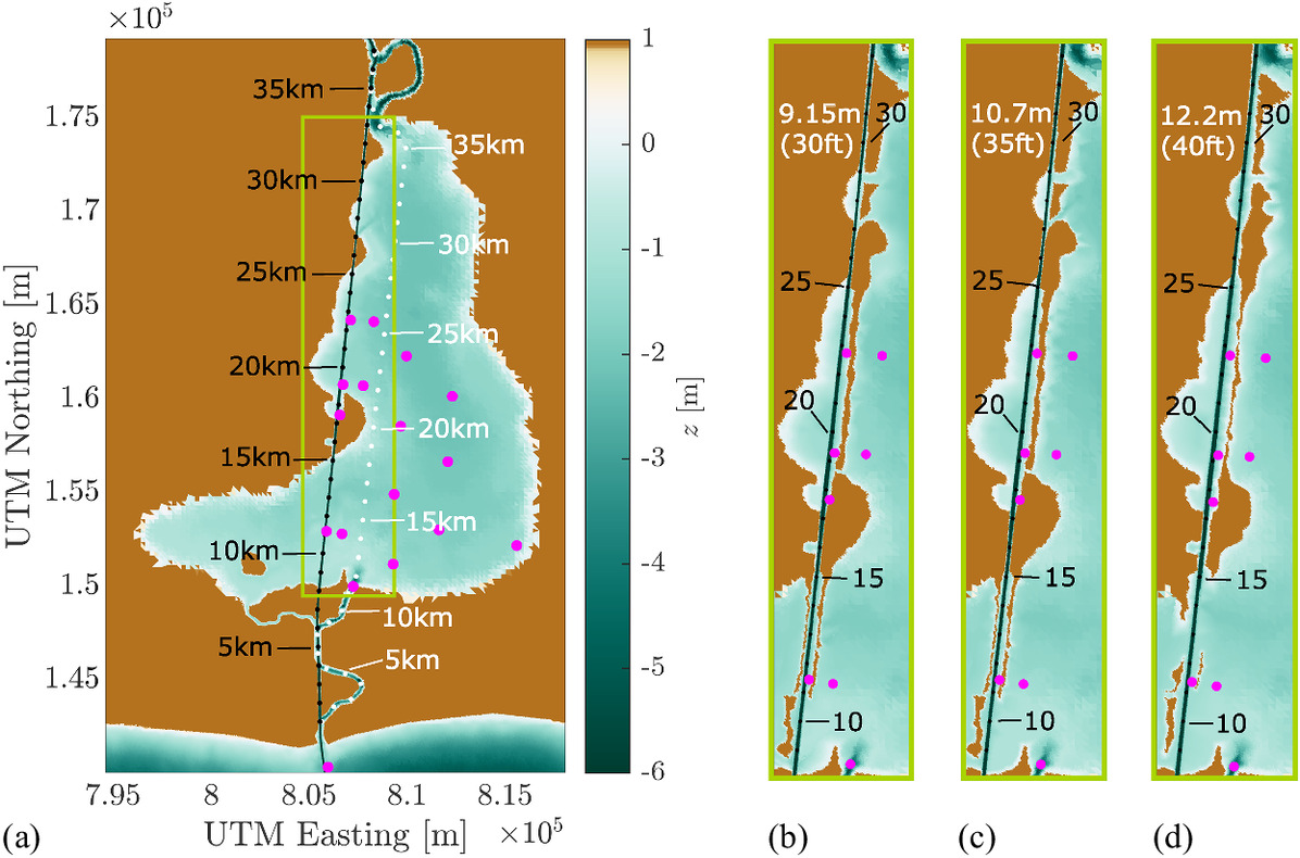
Computational meshes were derived from a number of sources to create a total of seven topobathymetric scenarios. Four of the tested scenarios were developed from the depths and contours illustrated in nautical charts for each stage of channel deepening, and three of the tested bathymetries are perturbations of the charted bathymetries (Table 1). Elevations were specified with georectified and hand-digitized nautical charts in the lake, river, and pass system (Fig. 3), and the NOAA NCEI Coastal Relief Model was used for offshore elevations. Outside of the pass and the main channel areas, the bathymetric grid was kept constant in an effort to constrain the experimental variables to channelization, deepening, and BUDM island formation. This was achieved by blending a combination of nautical charts across years, which indicated no substantial change in bathymetric conditions outside of the heavily managed regions of Calcasieu Lake, River, and Pass. For each deepening of the CSC, the Calcasieu River is equally deepened; for the prechannelization simulation, river depths north of the lake are set to 9.15 m (30 ft) based on the Chief Engineer’s 1883 Annual Report. Island boundaries (i.e., the wet/dry transitions) are numerically treated as vertical walls. Decadal scale topographic (i.e., subaerial) changes in channel-flanking island morphology are not well documented, and model results do not indicate large tide ranges outside of the pass and main channel (the Calcasieu system is microtidal), so the lack of wetting and drying over the linear islands is not likely to have a significant impact on the results of this work, though wetting and drying processes may be more important to incorporate in a process-based sediment transport modeling effort, particularly under high energy storm conditions.

Fig. 3. (a) Numerical model mesh elevations for Lake Calcasieu, where the white dots mark kilometers (km) upriver of the inlet in the pre-modified system, and black dots mark km upriver for the system following 1937. Green box shows focus region near BUDM islands for (b) 1938 following deepening to 9.15 m (30 ft); (c) 1948 following deepening to 10.7 m (35 ft); and (d) 1963 following deepening to 12.2 m (40 ft). Pink circles correspond to particle tracking source points.

Table 1. Description of topobathymetric configurations used for numerical modeling simulations, based on charted bathymetry (top row) and hypothetical bathymetry assuming channel-flanking islands were never built (bottom row) for four representative years

Topobathy configuration	1873	1938	1948	1963
Charted elevations	Initial deepening of Calcasieu Pass and Lake to maintain 1.98 m (6.5 ft) at MLLW	Linear channel authorized and dredged to depth of 9.15 m (30 ft); islands first present	Channel dredged to depth of 10.7 m (35 ft); islands present	Channel dredged to depth of 12.2 m (40 ft); islands present
Modified elevations (islands not present)	N/A	Hypothetical scenario in which all dredged sediment between 1873 and 1938 was placed in ODMDS	Hypothetical scenario in which all dredged sediment between 1873 and 1948 was placed in ODMDS	Hypothetical scenario in which all dredged sediment between 1873 and 1963 was placed in ODMDS

The three bathymetries that deviate from those depicted in nautical charts represent the hypothetical scenario in which all material dredged from the CSC was relocated offshore to ocean dredged material disposal sites (ODMDSs) rather than being used to construct near-channel islands (Table 1). For these bathymetric configurations, regions of the computational mesh previously occupied by islands were set to the mean water depth of the lake within approximately 30 m from the islands. These three hypothetical bathymetries are nearly identical to each other outside the depth of the CSC. Once developed, each of the seven bathymetric configurations described in Table 1 was applied as the unique bottom boundary conditions for the otherwise identical 30-day simulation.

Hydrodynamic forcing for the 30-day simulations represents seasonally averaged winter (January–March) conditions, which wave and meteorological observations indicated are on average the most energetic months. A one-day forcing ramp period is applied, yielding a 29-day simulation for analysis purposes. Wave statistics from NOAA National Data Buoy Center (NDBC) Station 42035 (depth of 15 m) and Station 42091 (depth of 21.6 m) were used to define normalized probability distribution functions (npdfs) of wave statistics for each winter on record (1993–2021 and 2021–2022, respectively). Averaging over the npdfs, the most probable winter significant wave height

H_{s}

, peak period

T_{p}

, and wave direction

θ_{p}

were calculated from the deep-water buoys and propagated to the model open boundary using linear wave theory, resulting in a JONSWAP spectral forcing condition with

H_{s}

of 0.8 m,

T_{p}

of 4.8 s, and

θ_{p}

of 18.7 degrees relative to the shore-normal axis. The amplitudes and phases of the eight dominant tidal constituents (per NOAA Tides and Currents Station 8768094) were mapped to the open ocean boundary from the TPXO database (Egbert and Erofeeva 2002) using the OceanMesh2D utility for Matlab (Roberts et al. 2019).

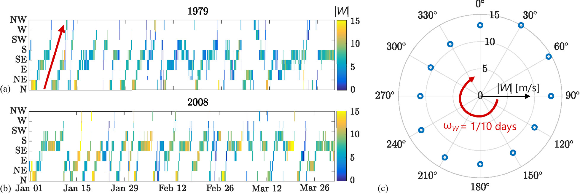
Streamflow at the riverine boundary was set to 132 m³ per second (m³/s), which was calculated to be the mean February flow rate observed at the USGS gauge at Kinder, LA (Station 08015500) over its historical record (1995–2023). Streamflow and wave conditions are kept temporally constant over the 30-day simulation period, while spatially uniform wind fields were varied temporally, as wind variability has been shown to dominate second-order circulation during winter and spring seasons in Lake Calcasieu, where the first-order mechanism are tides (Guo et al. 2020 and references therein). Frequent cold fronts switch the dominant wind direction from southerly to northerly, and occur roughly every 3 to 10 days between October and April (Guo et al. 2020). A similar periodicity in the wind fields is evident in measurements collected onshore (NOAA Tides and Current Station 8768094) as well as far offshore (NOAA NDBC Stations 42001 and 42002). The offshore meteorological station data were analyzed to calculate the 5% exceedance wind speed for 30-degree (°) directional bins and the frequency of rotation of the wind fields (

ω_{W}

) for the simulation period. Two sample winter time series of wind speed

| W |

and direction (cardinal and intercardinal) are provided in Fig. 4, as well as the directionally binned average 5% exceedance wind speed over the two buoy’s historical wind records (1973–2021).

Fig. 4. Sample winter (January–March) time series of wind speed $| W |$ (color bar, units of m/s) and direction (vertical axis) for (a) 1979; (b) 2008; and (c) average 5% exceedance wind speed for 30° directional bins. Red arrows in panels (a and c) indicate rotation of wind fields, which occur every 10 days in the computational simulations.

Salinity is not included in the model configuration because Lake Calcasieu’s shallow depths enable sufficient mixing (Waterways Experiment Station 1950; Meselhe and Noshi 2001; Brown and Luong 2022). Although the deep draft navigation channel does enable salinity intrusion as far inland as north of Lake Charles, the location of the salt wedge front and resulting estuary turbidity maximum (ETM) fluctuates substantially, largely attributed to the temporal variation in freshwater discharge (Waterways Experiment Station 1950). Lin et al. (2016) found that, during the 2011–2012 winter, the variability in salinity fluxes along the CSC due to changes in river discharge was twice the variability due to small perturbations in channel depth (

10.7 m \pm 1.5 m

). Thus, maintaining temporally constant streamflow at the inland model boundary reduces the need to include oceanic salinity fluxes for accurate system behavior. Additional considerations for the effect of salinity on the presented model results with implications for sediment transport are addressed in the section “Salinity and Shoaling Implications.”

Data Analysis

Based on the lack of currently available data needed to perform sediment transport simulations and explicitly compute the changes in shoaling rates due to the presence of channel-flanking islands, we instead use modeled wave and current velocities to identify how channel-flanking islands modify the hydrodynamic mechanisms and pathways of sediment transport.

Modification of Tidal Dynamics

Tidal asymmetry is calculated to determine whether net transport within the CSC is either ebb-dominant, leading to net seaward sediment transport, or flood-dominant, leading to net landward transport (Dronkers 1986; Brown and Davies 2010; Guo et al. 2019). Although previous works have defined tidal asymmetry by either an imbalance in tidal phase duration (ebb conditions lasting longer than flood conditions, or vice versa) or asymmetry in tidal velocities (peak ebb velocities exceeding peak flood velocities, or vice versa), Brown and Davies (2010) and Winterwerp and Wang (2021) demonstrated that asymmetry in both tidal wave duration and velocity magnitude should be evaluated to predict the direction of residual sediment fluxes. For example, if ebb current velocities are greater but brief compared with flood current velocities, bulk hydrodynamics cannot yield an adequate temporal integration to determine net transport direction. Following Brown and Davies (2010), we define duration asymmetry as the ratio of

T_{ebb}

to

T_{flood}

, where

T_{ebb}

(or

T_{flood}

) is the average duration of the ebbing (or flooding) tide in which the depth-averaged, channel-wise velocity is greater than the critical velocity for sediment transport

U_{cr}

, defined in the following section. For velocity asymmetry, we use the cubed ratio of the average peak ebb velocity

U_{ebb}

to average peak flood velocity

U_{flood}

, given the relationship between sediment transport and

U^{3}

(Guo et al. 2019; Eidam et al. 2020). When both

T_{ebb} / T_{flood} > 1

and

| U_{ebb} / U_{flood} |^{3} > 1

(or

T_{ebb} / T_{flood} < 1

and

| U_{ebb} / U_{flood} |^{3} < 1

), the longer erosive periods and stronger flow velocities during ebb (or flood) tide together provide a clearer indication of tidally averaged sediment fluxes (Brown and Davies 2010). Ebb- or flood-dominance can vary spatially throughout an estuary (Wang et al. 2002), and thus, positive or negative gradients in ebb- or flood-dominance can be used to qualitatively identify regions of sediment convergence (shoaling) or divergence (scouring).

Ebb and flood velocities

U_{ebb} and U_{flood}

are determined by reorienting the modeled velocity components

u

and

v

, which correspond to the horizontal (east) and vertical (north) Cartesian orientations. The dominant flow direction upstream, here referred to as the

x^{'}

direction, is at an angle

β

to the Cartesian horizontal and can be determined from principal component analysis (Jolliffe 2002). Flow parallel to the

x^{'}

-axis

U

is therefore equal to

u \cos β + v \sin β

. Because the hydrodynamics of the Calcasieu system are strongly influenced by wind forcing, tidal statistics are inferred from a spatially varying output time series after applying a 2-day moving average to remove the nontidal signal corresponding to the period of wind field rotation. After demeaning the

U

time series, a standard upcrossing routine was then used to find the average peak positive and negative values over all tidal cycles, which are used to define

U_{flood}

and

U_{ebb}

, respectively. To quantify the relative contribution of tidally driven currents to the total variation in velocity, we compute the ratio of the root mean square (RMS)

U_{tide}

to RMS

U_{total}

, where

U_{tide}

corresponds to the derived tidal time series and

U_{total}

corresponds to the unfiltered

U

time series.

Depositional Hotspots

Depositional hotspots are computed across the modeled domain from the entire month-long simulation, resulting in a spatially variable duration in which the total velocity is less than

U_{cr}

. In this analysis, the combined wave-current velocity

U_{wc}

(Lacy et al. 2007; Holzenthal et al. 2022) is tested against the critical threshold to account for potential suspension by modeled near-bed wave orbital velocities. The depositional hotspot analysis differs from the previously described tidal asymmetry analysis because it does not distinguish between ebb and flood velocities. In both the hotspot and tidal asymmetry analyses, a number of values for

U_{cr}

are considered to account for the range in possible sediment grain sizes making up the lake and channel bed. From previous work by Brown and Luong (2022), a fluid shear stress

τ_{cr}

of 0.125 pascals (Pa) is sufficient to suspend silts or clays from the sediment bottom. The equivalent velocity required for suspension can be found to be, on average, 0.27 m/s using the formula

U_{cr} = \sqrt{τ_{cr} / ρ C_{d}}

, where

ρ

is the fluid density and

C_{d}

is dependent on bottom friction conditions and the time-varying water depth (Soulsby 1997; Holzenthal et al. 2022). In this work, depositional conditions are defined as

U_{wc} < U_{cr}

, and the duration contours calculated from each simulation are used to calculate the change in the duration of depositional conditions due to the presence of the channel-adjacent islands for each CSC depth.

Particle Tracking Model

Finally, we use the modeled current vectors and water surface elevations to run Particle Tracking Model (PTM) simulations (MacDonald et al. 2006). PTM was developed to perform Lagrangian particle tracking analyses to monitor containment and sediment transport using a fourth-order Runge–Kutta approximation scheme (Gailani et al. 2016; Lackey et al. 2018). In the PTM simulations performed for Lake Calcasieu, point sources are distributed across the domain at 17 various locations [pink circles, Fig. 3(a) see online publication for color version of figure], including outside the inlet, throughout the open waters of the shallow lake, and along the channel- and lake-facing edges of the BUDM islands. Neutrally buoyant particles are released at four different times during the 30-day period, each corresponding to a different dominant wind direction. From the PTM-modeled pathlines, we define settling to occur between 20 h (hours) and 36 h after dispersal, based on previous simulations in which settling rate was defined as

1 \times 10^{- 5}

m/s (Brown and Luong 2022). The total number of particles, from each of the 17 source locations, residing within binned portions of the navigation channel averaged over the settling period are computed for each of the four dispersal intervals.

Results

Modification of Tidal Dynamics

The channelization and deepening of Calcasieu Pass through Lake Calcasieu enables tidal energy to propagate further landward from the inlet, as opposed to the pre-channelization configuration [Fig. 5(a)]. Prior to channelization, the relative contribution of the tide to the total variation in along-channel velocity was roughly 40% (RMS

U_{tide}

/RMS

U_{total} \approx 0.4

) between the inlet and a distance of approximately 13 km landward [see white dots in Fig. 3(a)], beyond which the tidal contribution was as little as 10% [Fig. 5(a)]. After channelization and deepening, variation in along-channel velocities due to the tides is found to be responsible for more than 90% of the total variation in velocity between the inlet and a distance of approximately 5 km for all channelized and deepened model configurations [Fig. 3(a), black dots]. At distances between 5 and 8.5 km, tidally derived variation in

U

drops to roughly 80%. Beyond distances of 8.5 km, the tidal contribution to variation in along-channel velocities drops to roughly 30%, indicating another time-varying forcing exerts greater control on the velocity signal. The drop in tidal contribution is found to be more gradual and falls to a lower value (less than 10%) when islands are not present [Fig. 5(a), dashed lines]. The 12.2 m with-island configuration has the most gradual transition from large (70%) to small (15%) tidal contribution. When the islands are present, the relative variance in velocity due to the tides stays within 15%–25% of the total velocity variance and remains fairly constant beyond upstream distances of roughly 15 km, as compared with the no-island cases in which tidal contribution falls nearly monotonically with upstream distance.

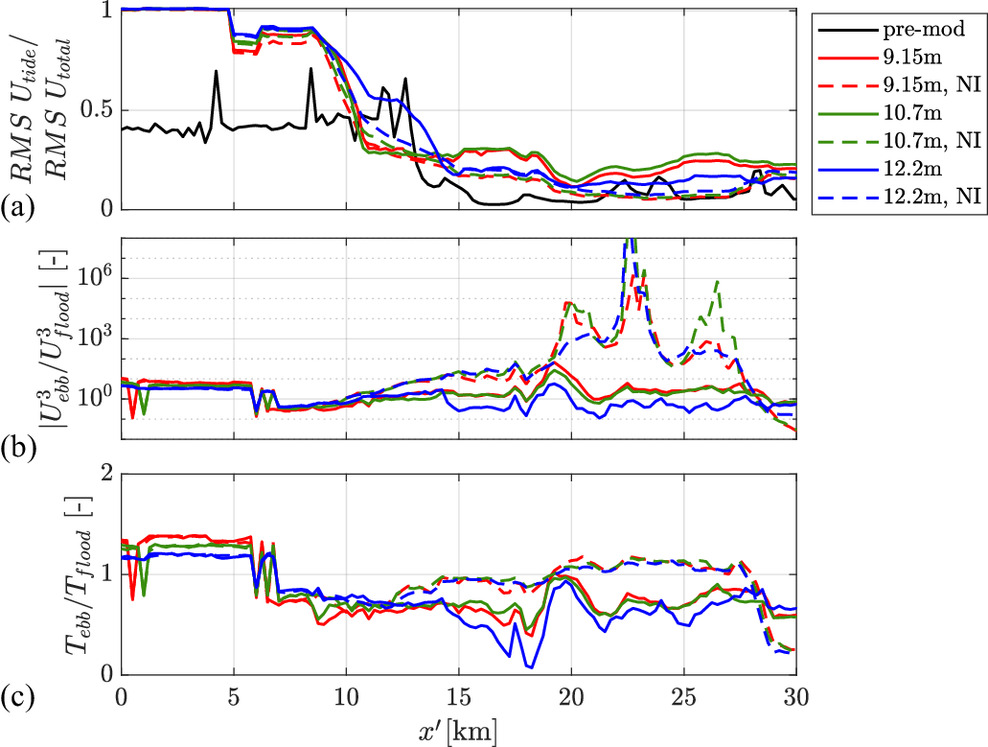
Fig. 5. Along-channel tidal statistics calculated from month-long simulation output (channel distance markers are shown in Fig. 3). Line color corresponds to unique channel depth, solid lines denote historical bathymetry, and dashed lines correspond to modified bathymetry with no islands (NI): (a) ratio of RMS tidal velocity ( $U_{tide}$ ) to RMS total velocity ( $U_{total}$ ); (b) peak ebb–flood velocity ratio $| U_{ebb} / U_{flood} |^{3}$ ; and (c) total amount of time during ebb tide in which the wave-current velocity $U_{wc}$ exceeds the critical velocity $U_{cr}$ ( $T_{ebb}$ ) normalized by the time during flood in which $U_{wc}$ exceeds $U_{cr}$ ( $T_{flood}$ ).

Along-channel variation in ebb or flood dominance [Figs. 5(b and c)] was found to be fairly consistent for all bathymetric configurations up to distances of approximately 11–12 km from the inlet: from the inlet to a distance of approximately 6 km, ebb tides dominate both in intensity (

U_{ebb}^{3} / U_{flood}^{3} > 1

) and duration of transport (

T_{ebb} / T_{flood} > 1

), whereas flood tides dominate in both intensity (

U_{ebb}^{3} / U_{flood}^{3} < 1

) and transport duration (

T_{ebb} / T_{flood} < 1

) at distances between 6 and 11–12 km. Beyond upstream distances of 12 km, trends in ebb–flood dominance vary significantly between with-island and no-island configurations. When the islands are not present, cubed values of peak ebb velocities (

U_{ebb}^{3}

) are orders of magnitude greater than cubed values of peak flood velocities (

U_{flood}^{3}

); additionally, erosive conditions are on average equal for ebb and flood tides, though there is a slight preference for ebb-directed erosion at channel distances where

U_{ebb}^{3} / U_{flood}^{3}

is greatest. In contrast, for the with-island configurations,

U_{ebb}^{3} / U_{flood}^{3}

hovers around 1 at distances upstream of 12 km, but

T_{ebb} / T_{flood}

is consistently less than 1.

Depositional Hotspots

Spatial contours of the change in total time (over the month-long simulation) that depositional conditions are met are provided in Fig. 6, where red areas indicate an increase in time depositional conditions were met due to the islands’ presence, and blue areas indicate a decrease in depositional conditions. Between upstream distances of 8 and 10 km, where the CSC only has a near-channel island on its western bank, the islands lead to a slight increase in depositional conditions when the CSC is 9.15 and 10.7 m, but no significant changes when the CSC is 12.2 m deep. Between upstream distances of 10 and 15 km from the inlet, depositional conditions are reduced by as much as two days when the islands are present for the 9.15 and 10.7 m depths, when the CSC has linear islands on both sides of the channel, but less if any change in depositional conditions are found in this section of the CSC for the 12.2 m channel configuration when islands have much larger gaps between them on the western bank and are nearly absent on the eastern bank. Regardless of depth, just outside the CSC, depositional conditions are shown to increase and then decrease at the island boundaries, where present. Between upstream distances of 15 km and roughly 18 km, where the CSC is tightly bounded through a cutoff formed during initial channelization, depositional conditions consistently increase due to the presence of the linear, channel-flanking islands, regardless of CSC depth. Note that in the no-island configurations, the cutoff between

x^{'} = 15

and

x^{'} = 18

km is still bounded by the original lake geography [Fig. 3(a)].

Fig. 6. Change in total amount of time (over month-long simulation) during which depositional conditions are met due to the presence of channel-adjacent islands, calculated as the difference in duration between configurations with and without islands for (a) main channel depth of 9.15 m; (b) main channel depth of 10.7 m; and (c) main channel depth of 12.2 m; red contours (colorbar) correspond to an increase in duration of depositional conditions due to island presence, and blue contours correspond to a decrease in duration of depositional conditions. Along-channel distances (in km) are noted (see Fig. 3 for reference).

Particle Tracking Model

The total number of particles (

N p

) settling within the main channel found by PTM analysis includes the length of the CSC up to a distance of 33 km from the inlet. The

y

-axis in Fig. 7 corresponds to the average

N p

within the channel over the settling period, and the error bars correspond to the standard deviation, where each marker color–shape combination represents a unique topobathymetric configuration. Because rotational wind fields have been shown to play a strong role in Lake Calcasieu hydrodynamics, each panel of Fig. 7 shows the average number of particles settling within the CSC for four different instances of dispersal, which correspond to prevailing winds toward each of the four cardinal directions. Over the 20 to 36 h prior to particle settling, winds continuously shift in a clockwise rotation (Fig. 4), meaning that the particles settling within the channel shown in Fig. 7(a) are exposed to winds blowing toward the east and southeast, particles depicted in Fig. 7(b) are exposed to winds blowing toward the south and southwest, and so forth for Fig. 7(c) (winds to the west and northwest) and Fig. 7(d) (winds to the north and northeast). For almost all wind conditions, more particles are found to settle into the CSC when the islands are present than when the islands are absent. However, the difference in

N p

between the with- and without-island configurations does vary significantly depending on the dominant wind direction and the channel depth-island morphology combination. For example, particle settling into the CSC was greatest when winds were blowing toward the east and shifting to the southeast [Fig. 7(a)] for both the with-island case (between 1324 and 1439 particles) and no-island case (between 1,002 and 1,187 particles). In contrast, when winds were blowing toward the south and shifting to the southwest [Fig. 7(b)] and when winds were blowing toward the west and shifting to the northwest [Fig. 7(c)], the islands enabled much more settling into the CSC than the no-island configuration for the 9.15 and 10.7 m depth configurations than the 12.2 m depth configuration. In fact, when the winds were blowing to the west and northwest, island presence resulted in no significant difference between particle settling into the CSC for the 12.2 m channel depth.

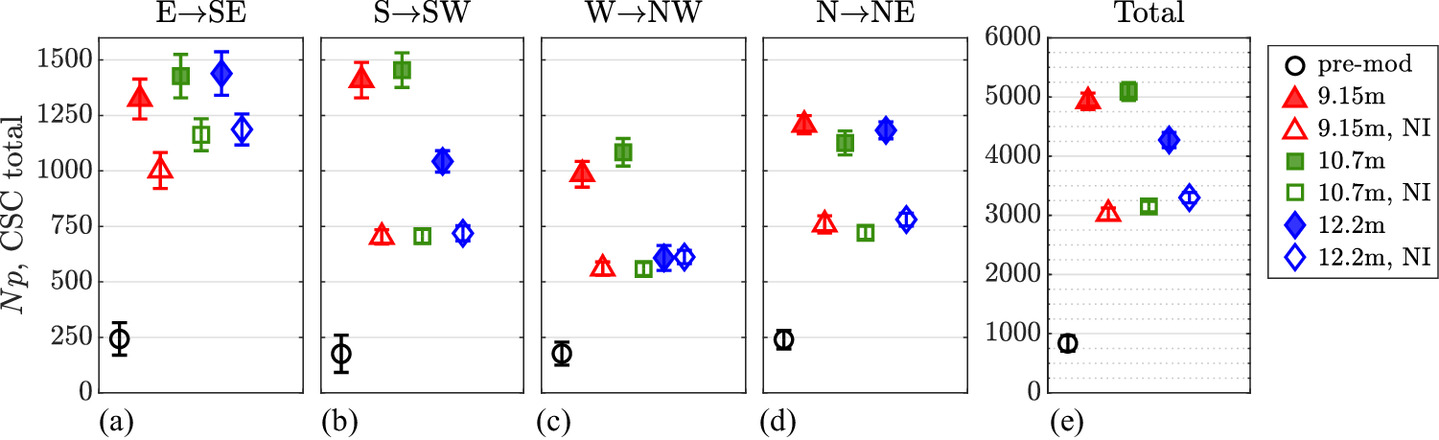
Fig. 7. Total number of particles ( $N p$ ) in the CSC, averaged over the settling period, for each bathymetric condition (marker color and shape, where NI indicates the no-island case) when particles are dispersed as: (a) winds shift from E to SE; (b) winds shift from S to SW; (c) winds shift from W to NW; (d) winds shift from N to NE. Total over all wind conditions shown in panel (e).

Fig. 8 shows spatial variability in the change in particle settling when the islands are present compared with when the islands are absent, where the red shading indicates where the islands increase particle settling within the channel, and blues indicate where the islands protected the main channel from settling particles. The circles in Fig. 8 are colocated with particle point sources (PSs), and their relative size indicates the change in the number of particles from that source that settle within the channel; blue circles indicate a decrease in number of particles from that source when the islands are present and red indicates an increase in number of particles from the source. For illustrative purposes, Fig. 8 only presents the results for two wind directions for two different CSC depths, as the figures illustrating the spatial patterns in sources and sinks were qualitatively similar for the 9.15 and 10.7 m depth configurations. Generally, the islands are revealed to block particles from the west (lake-facing) side of the channel in the upper portion of the CSC, such as from PS2 and PS4. However, the islands are also revealed to trap particles sourced from the eastern (channel-facing) side of the islands, such as material potentially eroded from the islands themselves, depending on the wind direction and island continuity.

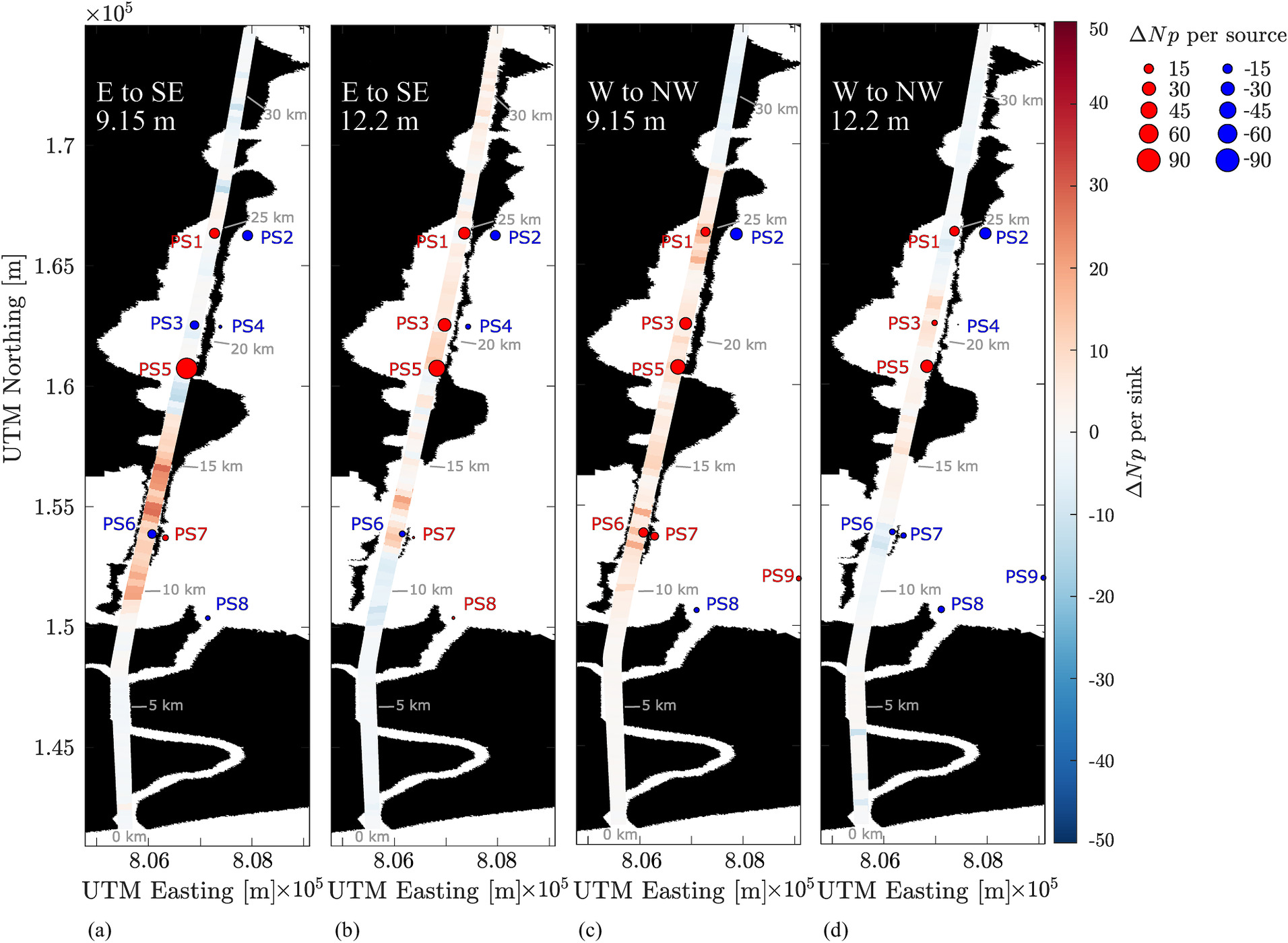
Fig. 8. Change in number of particles settling into the CSC, partitioned into 250 m bins (colorbar), due to channel-adjacent islands for (a) 9.15 m channel for winds blowing toward the E and SE; (b) 12.2 m channel for winds blowing toward the E and SE; (c) 9.15 m channel for winds blowing toward the W and NW; and (d) 12.2 m channel for winds blowing toward the W and NW. Change in number of particles by source presented as scaled circles, where an increase in particles settling in the channel from a given point source (PS) is in red, and a decrease in particles is in blue.

For example, when winds are blowing to the east and southeast, a small gap between islands (near PS5) [Fig. 8(a)] enables more of the particles from PS3 to exit when the islands are present; nautical charts evidenced this gap when the CSC was maintained at 9.15 m and 10.7 m but not at the 12.2 m depth. When this gap is absent for the 12.2 m depth configuration, the islands lead to more retention of particles in the CSC than the no-island case [Fig. 8(b)]. Similarly, once particles reach the portion of the channel between 8 km and 15 km from the inlet, the more continuous islands present for the 9.15 m and 10.7 m depth configurations trap more particles in the channel than in the islands in the 12.2 m configuration, which are fewer and spaced further apart. The islands are again shown to retain more particles between upchannel distances of 8 km and 15 km when winds are blowing to the west and northwest and the islands are more continuous in the same area [Fig. 8(c)] than when the islands are less continuous [Fig. 8(d)]. Furthermore, when the winds are blowing toward the west and northwest, PS6 and PS7 in the lower half of the lake are the source of more particles in the channel when the islands are continuous than when they are not, in which case the discontinuous islands actually lead to fewer particles from PS6 and PS7 than when the islands are absent. It is additionally evidenced that material released from and/or suspended at point sources nearly 3 km from the channel [PS9 in Fig. 8(c)] can be a source of particles settling within the channel when the winds are directed toward the west and northwest, where they become more trapped when the islands are present and continuous than when the islands are present but discontinuous.

Discussion

This work investigates two different scales of mechanisms through which channel-adjacent BUDM islands could modify shoaling patterns. At the spatial and temporal scale of tides, the islands do appear to increase the likelihood of shoaling in some portions of the CSC, but only within regions that coincidentally have relatively low tidal influence. At the local scale, island presence and continuity can shift sediments toward or away from the CSC, but these pathways can be difficult to predict on longer time scales, as they appear to be highly sensitive to wind conditions as opposed to predictable forcing cycles (i.e., tides). The implications for shoaling of channel-adjacent islands at these two scales are discussed in greater depth in the following sections.

Shoaling Implications from Large-Scale Hydrodynamics

Overall, modeled combined wave-current velocities indicate that the section of the CSC most likely to experience increased shoaling due to the presence of the parallel, near-channel BUDM islands is located between 15 and 19 km from the inlet. For comparison with historical nomenclature, this section corresponds to river mile (RM) 8 through 11. This section of the CSC is shown to be bounded between two large land masses, which are present in all six postmodification topobathymetric configurations (Table 1). Even so, the red shading in this portion of the CSC indicates that the channel-adjacent islands do increase the duration of the simulation in which

U_{wc} < U_{cr}

(Fig. 6). Thus, the islands to the north and south of these landmasses, rather than purely the landmasses themselves, result in a net decrease in flow velocities in this area such that depositional conditions increase compared with the no-island configurations. The velocity reduction between

x^{'} = 15 km

and

x^{'} = 19

km by the islands could be due to increased frictional dissipation; though not shown, average peak flood velocities at the same section of the CSC increase by no more than 5 cm/s when the islands are present, but average peak ebb velocities decrease in magnitude when the islands are present by nearly 7 cm/s for the two shallower channels depths (9.15 m and 10.7 m) and by more than 15 cm/s for the deepest channel depth (12.2 m). Recent physical observations by Perkey et al. (2022) report a layer of fluid mud in this area with a thickness between 0.6 m and 1.8 m. Process-based sediment transport modeling by Brown and Luong (2022) also support the presented findings that depositional conditions are more prevalent on the shallow banks of the CSC when the islands are present although much of the CSC itself, outside of

x^{'} = 15

–19 km, is found to have decreased duration of depositional conditions when the islands are present (Fig. 6). Results of the numerical modeling by Brown and Luong (2022) indicate sediment accretion rates in these shallow reaches between the CSC and channel-flanking islands can be as high as 0.5 m/yr.

The depositional-prone section of the CSC between 15 km and 19 km from the inlet is also found to be colocated with a region of tidal convergence. In Figs. 5(b and c), there is a positive slope in

| U_{ebb} / U_{flood} |^{3}

and in

T_{ebb} / T_{flood}

for the three postchannelization configurations when islands are present between 17 km and 20 km upstream. In this section of the CSC,

| U_{ebb} / U_{flood} |^{3}

switches from less than 1 to greater than 1 for the 12.2 m depth with-island configuration, and the ratio increases from 1 to greater than 1 for the 9.15 m and 10.7 m depth with-island scenarios, noting that the vertical axis scale is logarithmic [Fig. 5(b)]. In the same location,

T_{ebb} / T_{flood}

increases from 0.1 to nearly 1 for the 12.2 m depth with-island scenario and from roughly 0.5 to 1 for the shallower depth cases with islands present [Fig. 5(c)]. The combined observations indicate that tidally driven sediment fluxes shift from strongly flood dominant (landward) to near equal if not definitively ebb dominant (seaward). A loss of flood-dominance with increasing

x^{'}

leads to net accumulation in sediment. The alignment of the positive gradient in ebb-to-flood ratios with time-averaged increases in depositional conditions (Fig. 6) indicates that quantifying changes in large-scale hydrodynamics by the channel-adjacent islands can be used to qualitatively identify regions likely susceptible to shoaling. This interpretation of channel-wise hydrodynamic metrics as a convergence zone is supported by the observed decrease in ebb velocities when the islands are present at upstream distances

x^{'} > 15

km, particularly for the deepest channel depth, which was shown to have the greatest increase in depositional conditions due to island presence as well as the largest gradient in

T_{ebb} / T_{flood}

. While the no-island configurations do show a slightly positive gradient in

T_{ebb} / T_{flood}

when the islands are not present, the gradient is larger when they are present, indicating a greater accumulation in material when the islands are present than when they are absent.

The negative gradient in

T_{ebb} / T_{flood}

and, to a lesser degree,

| U_{ebb} / U_{flood} |^{3}

for the with-island configurations between upstream distance of 15 km and 17 km, immediately preceding the positive gradient, are indicative of a sediment divergence zone or increased likelihood of scour; the blue shading south of the cutoff in Fig. 6 is similarly indicative of decreased depositional conditions when the islands are present.

Interestingly, the section of the CSC between 15 km and 19 km from the inlet, which the results show to be more depositional when islands are present and that converging tidal fluxes are a contributory mechanism, is also found to be a section of the CSC where tidal processes exhibit relatively little control on local hydrodynamics [Fig. 5(a)]. In the presented numerical simulations, streamflow conditions were held constant and wind fields rotated in full 360-degree cycles at a constant rate [Fig. 4(c)]. However, in reality, streamflow and particularly wind fields may vary nonuniformly over a 30-day period. Because the tidal contribution to total velocity variability in the upper section of the CSC (

x^{'} > 15

km) is only found to be between 20% and 30%, the time-averaged depositional conditions in this portion of the CSC may be sensitive to variable wind and streamflow conditions. In other words, the calculated sediment convergence and divergence caused by gradients in tidal asymmetry may not always be well correlated with monthly mean depositional conditions in this portion of the CSC. While variability in streamflow and wind conditions averaged over annual and decadal time scales may lead to long-term accretion by tidal mechanisms, it is expected that changes in coastal meteorology and rainfall caused by warming oceans will likely impact the balance of tidal, riverine, and wind-stress mechanisms of sediment transport in the upper reaches of the CSC.

Shoaling Implications from Local-Scale Hydrodynamics

The results of the particle tracking analysis indicate that the islands can act to either block material from entering the CSC, leading to decreased shoaling potential, or trap material within the CSC, leading to increased shoaling potential. Furthermore, these functional capacities are not mutually exclusive and are dependent on diurnal scale forcing conditions (Fig. 8). Gaps between islands in particular are found to play a critical role as exit points for material suspended on the channel-facing edge of the islands, provided hydrodynamic conditions direct the flow toward the gaps. A clear example of this is evident in comparing particle trapping by islands in the 9.15 m depth configuration [Figs. 8(a and c)]. In Fig. 8(a), particles dispersed from PS3 appear to be forced out of the channel between the gap near PS5, but in Fig. 8(b), wind forcing directly opposes the flow direction required for exit through the gap. This small gap/high continuity island configuration appears to provide both strong blocking and trapping functions but was ultimately found to lead to more particles trapped within the channel when the islands are present (Fig. 7). In contrast, for the 12.2 m depth configuration, the channel-adjacent islands between 8 km and 15 km from the inlet are smaller in length and have larger gaps between them; for the east-directed and west-directed dispersals, far fewer particles settled in this section of the CSC between the islands as compared with the 9.15 m depth configuration with larger islands closer together. Given that the islands vary little upstream of

x^{'} = 15

km across depth-configurations (excluding one narrow gap that is absent for the deepest depth configuration), it is likely the sparse island configuration south of

x^{'} = 15

km leads to overall decreased particle retention as compared with the with-island configurations with shallower depths (Fig. 7). In fact, despite the long continuous island north of

x^{'} = 15

km for the deepest channel condition, no statistical difference was found between the total number of particles settling in the channel for the island and no-island configurations when winds were to the west, and the difference between the with- and without-island configurations was much less than the difference between them for shallower depths when the winds were to the south.

Due to the sensitivity of the PTM results to wind conditions (Figs. 7 and 8), we expect the numeric quantities of total number of particles settling in the channel to change should the wind conditions change. The PTM results also assume that sediment has an equal likelihood of suspension and/or dispersal across all tested point sources (Fig. 3, pink circles), which may not reflect reality. However, we did observe increased duration of erosional conditions along the channel-facing sides of the BUDM islands (not shown), which spatially corresponds to the blue shaded areas on the channel-facing side of the BUDM islands to the east of the CSC (Fig. 6). Based on the findings of the depositional hotspot analysis and previous studies (Perkey et al. 2022; Brown and Luong 2022), some of the material eroded from the island edges may fall out of suspension before reaching the channel. Thus, not only could the islands act as a source of sediment, but their linear, continuous form likely blocks wave, tidal, and wind energy from refracting around them, creating large shadow zones that enable deposition. Finally, we also note that although the results show that material suspended 5 km from the islands is expected to reach the CSC within the 20–36 h settling period, this does not mean that material from more distant point sources (Fig. 3) could not contribute CSC shoaling rates. While not shown, the PTM results showed that the system becomes fairly well-mixed in terms of particle distribution from all sources within the month-long simulation when the particles are assumed to be neutrally buoyant (i.e., no settling enabled), which is consistent with previous observations of salinity fluxes in the lake and channel system (Meselhe and Noshi 2001; Lin et al. 2016).

Salinity and Shoaling Implications

The inland-most point of salinity intrusion is associated with the estuary turbidity maximum (ETM); turbulent mixing at the boundary between the salt wedge and freshwater discharge keeps bed material in suspension, creating a fluid mud layer. Thus, predicting the ETM position can inform channel sediment management, but doing so requires a fully three-dimensional multilayered numerical model to resolve the salinity gradient at the salt wedge front, which is particularly challenging for the case of the highly stratified salinity front evidenced in the CSC (Lin et al. 2016). However, as discussed in the section “Numerical Modeling,” salinity is not included in the CMS modeling performed for this analysis because its focus is limited to the effect of the BUDM islands. A previous modeling study performed by Lin et al. (2016), which included salinity and baroclinic effects, found that the variation in salinity fluxes along the CSC due to variation in river discharge was twice the variation due to small perturbations in channel depth (

10.7 m \pm 1.5 m

). Although they did not isolate the effect of the BUDM islands, their findings suggest the absence of islands may slightly shift the position of the salt wedge front and ETM, but the bathymetric gradient between the shallow lake and the deep channel is sufficient to maintain strong stratification without the islands (Lin et al. 2016). Without speculating as to the limit of salinity intrusion for the scenario modeled herein, it is difficult to infer whether the small potential shifts in ETM by island “removal” would occur within the region of interest (within 35 km of the inlet). To fully resolve the salinity front is nontrivial and would require a depth-resolving, highly resolved (in space and time) numerical model (Lin et al. 2016), which is beyond the scope of this work. Such a model could be used to identify to what degree the islands inhibit mixing. Although we hypothesize that any mixing enabled by the islands’ absence may not be sufficient to disrupt the strong density gradient in the Calcasieu system, it is possible that islands along deep draft channels in deeper water bodies more substantially inhibit mixing and have a greater potential to shift the salt wedge and ETM.

Conclusions

The beneficial use of dredged material (BUDM) collected during navigation channel deepening for increased species habitat has previously been studied for its impacts to environmental quality. Yet the impact of these placements (10s of km) to system-scale hydrodynamics (100s–1,000s of km) has been largely overlooked, particularly when BUDM islands are located very close to the navigation channel. This work investigates how channel-parallel linear island features may modify various sediment transport mechanisms and pathways. Based on the various tested channel and embayment geometries, taken from nautical charts detailing the evolving topobathymetric history of Lake Calcasieu and the Calcasieu Shipping Channel (CSC), linear and near-continuous islands have the potential to increase sedimentation in the channel by altering both local hydrodynamics and estuarine-scale tidal statistics. In addition to trapping particles within the confines of the navigation channel, hydrodynamic modeling results indicate that the islands can modify tidal dynamics along the length of the channel such that a zone of converging ebb- and flood-tide sediment fluxes can form; for the same navigation channel depth without near-channel islands, sediment convergence is expected to be reduced, if it occurs at all. Furthermore, results from particle tracking modeling show that even small gaps between islands can permit redirection of material suspended at the channel’s edge, such as by island erosion or by vessel wake, toward the open embayment and away from the navigation channel. The modeled results indicate that tidally averaged hydrodynamics (i.e., gradients in ebb and flood dominance) may be able to predict regions of sediment convergence in the case of equally distributed wind fields and constant streamflow conditions, which were found to be larger contributors to variability in along-channel velocities than tidal fluctuations in the upper portion of the CSC. Findings also suggest that greater spacing between islands may reduce the amount of material generated from or near the islands from re-entering the navigation channel.

Data Availability Statement

The Coastal Modeling System (CMS) and the Particle Tracking Model (PTM) are available in the community version of the Surface-water Modeling System (SMS), which can be found at https://www.aquvaveo.com. The CMS source code is also available at https://github.com/erdc/cms2d. Modeled hydrodynamic data and processing scripts can be made available from the corresponding author upon reasonable request.

Acknowledgments

The authors wish to acknowledge the US Army Corps of Engineers (USACE) Coastal Inlets Research Program (CIRP) for funding this research, as well as Tanya M. Beck (CIRP Program Manager); Jeff Corbino and the USACE New Orleans District for their feedback; Mitchell Brown, Honghai Li, and Lihwa Lin of the USACE Coastal & Hydraulics Laboratory Coastal Modeling System (CMS) team for their support.

Author contributions: Conceptualization – D.R.K., R.L.B.; Data curation – R.L.B., E.R.H., D.R.K.; Formal analysis – E.R.H., R.L.B.; Investigation – E.R.H., R.L.B., D.R.K.; Methodology – E.R.H., R.L.B., D.R.K., R.B.S, J.A.C.; Supervision – R.B.S.; Visualization – E.R.H., J.A.C.; Writing, original draft – E.R.H., R.L.B.; Writing, reviewing and editing – D.R.K., J.A.C.

References

Amin, M. 1983. “On perturbations of harmonic constants in the Thames Estuary.” Geophys. J. Int. 73 (3): 587–603. https://doi.org/10.1111/j.1365-246X.1983.tb03334.x.

Abstract

Introduction

Background

Methodology

Numerical Modeling

Data Analysis

Modification of Tidal Dynamics

Depositional Hotspots

Particle Tracking Model

Results

Modification of Tidal Dynamics

Depositional Hotspots

Particle Tracking Model

Discussion

Shoaling Implications from Large-Scale Hydrodynamics

Shoaling Implications from Local-Scale Hydrodynamics

Salinity and Shoaling Implications

Conclusions

Data Availability Statement

Acknowledgments

References

Information

Published In

Copyright

History

ASCE Technical Topics:

Authors

Affiliations

Metrics

Citations

Download citation

Figures

Other

Share

Copy the content Link

Share with email

Share

Request Username

Create a new account

Change Password

Password Changed Successfully

Verify Phone

Congrats!