Cloud-Based Platoon Predictive Cruise Control Considering Fuel-Efficient and Platoon Stability
Publication: Journal of Transportation Engineering, Part A: Systems
Volume 150, Issue 3
Abstract
This work investigates commercial vehicle platoon predictive cruise control for highways. We propose a cloud-based platoon predictive cruise control method (CPPCC). A two-layered control architecture of the CPPCC is proposed as a platoon predictive cruise speed planning layer in the cloud and a platoon stabilization control layer. The CPPCC communication topology is proposed to achieve coupled control of the hierarchical architecture. The speed planning layer is a dynamic planning (DP) algorithm based on road slope in the rolling distance domain. The lower layer is a stability control algorithm to meet the stability requirements of vehicle platoon driving; the vehicle side is distributed model predictive control (DMPC). The CPPCC is validated by real road and vehicle data models, and comparative experiments with the traditional predecessor-leader following–cruise control (PLF-CC) platoon and predecessor following–cruise control (PF-CC) platoon. The speed error of the vehicle platoon was maintained at [, 0.30] () and the space error at [, 0.66] (m) in platoon stability. Against the comparison method, the CPPCC saved fuel by over 5.13% and achieved an overall operational efficiency improvement of 5.71%.
Practical Applications
This research contributes to solving the problem of energy-efficient driving in vehicle platoons. Based on the cloud control system (CCS), cloud-based platoon predictive cruise control (CPPCC) is proposed, which is a layered structure. The upper layer is the platoon speed planning layer in the cloud and the lower layer is the platoon stability control layer. By adding cloud nodes and changing the structure of the existing platoon predictive cruise control (PPCC) and communication topology, CPPCC is able to achieve the goals of platoon economy and stability. Compared with PF-CC and PLF-CC, it is able to achieve fuel savings of more than 5.13% and efficiency improvements of 5.71% while ensuring stable platoon operation. Deploying the vehicle-side platoon stabilization controller in a commercial vehicle platoon can provide a solution to existing PPCC for energy saving and stability control. Combined with cloud-based speed planning, this enables commercial vehicle platoon PCC. Solving the problem of energy consumption of existing commercial vehicles and thus reducing environmental pollution from logistics transport.
Introduction
The rapid development of road transport has brought several serious challenges, such as traffic safety and environmental pollution. Commercial vehicles are the mainstay of road transport and their energy consumption and safety problems are becoming increasingly serious. There is an urgent need for a way to ensure safe driving, reduce energy consumption in freight transport, and improve transport efficiency. An effective way of solving this problem is to organize vehicles into closely spaced vehicle platoons. Various roadside equipment has been built and gradually improved with the advancement of communication technology. The application and rapid progress of vehicle-to-vehicle communication (V2V), vehicle-to-road communication (V2R), and other technologies can provide strong technical support for vehicle platoons. Multivehicle cooperative formation technology in intelligent transportation systems (ITSs) will have significant social and economic value in improving vehicle transportation efficiency, driving safety, energy savings, and emissions reduction.
Due to the practical needs of commercial vehicle platoons and the potential for energy savings, several countries and regions have started research into heavy commercial vehicle platooning technology, and commercial vehicle platoons are now the focus of research. Especially for high-speed scenarios, commercial vehicle platoons can be optimized and controlled using information such as road slope, curvature, and traffic flow, or by reducing platoon spacing to reduce wind resistance.
Studies have shown that reducing overall air resistance using a platoon can reduce overall energy consumption. However, there are differences in the reduction of air resistance between vehicles in different positions in the platoon. Commercial vehicles can save 10%–15% fuel consumption at a platoon spacing of 10 m (Guo and Wang 2019), but too a small distance between vehicles in a high-speed platoon can lead to safety problems, so a more practical research focus is vehicle platoon predictive cruise energy-saving driving control.
Platooning studies are designed to reduce the energy consumption of vehicle platoons. However, the vehicle platoon is a mutually coupled complex system, and changes in the speed of the vehicles in it may lead to instability of the system. The speed fluctuations of the vehicles in front of the platoon will be amplified back along the platoon step by step, causing frequent acceleration and deceleration to ensure string stability. However, frequent acceleration and deceleration will result in higher fuel consumption. A great deal of research has been done on the stability of the platoon, with more focus on the sliding mode controller (SMC) and the model predictive controller (MPC) approaches.
The SMC has the advantage of dealing well with nonlinear dynamical systems, actuator limitations, and diverse communication topologies, and is insensitive to external perturbations. Scholars have focused more on the SMC design in different communication topologies and spacing strategies, and on eliminating jitter as the system plateaus (Yu et al. 2018; Guo et al. 2017; Wu et al. 2020).
Three technical features of MPC—namely predictive model, rolling optimization, and feedback correction—solve the problem of platoon stability. MPC has been applied to platoon stability control by a large number of scholars. Yu et al. (2016) proposed MPC in considering ramp information for hybrid electric vehicle platoons, which can effectively reduce energy consumption. Zheng et al. (2017) proposed a distributed MPC (DMPC) to ensure platoon stability for heterogeneous vehicle platoons with unidirectional topology and a priori heterogeneous vehicle platoons with unknown desired set points. Kazemi et al. (2018) proposed a learning-based driver behavior modeling approach in combination with MPC to improve the overall performance of cooperative adaptive cruise control (CACC).
Research into the control architecture for platoon predictive cruise control (PPCC) has included both hierarchical and centralized approaches. The centralized scheme requires status information of all vehicles in the platoon, has high communication requirements, and is difficult to design. The hierarchical solution has a clear design logic, is less difficult to design, and is easy to implement. It is now the mainstream platoon control architecture. For the upper layer of platoon decision planning, the main problem is the planning of economic vehicle speed. Under the premise of ensuring the safety and stability of the platoon, the lower-layer controller completes the policy following control of the upper-layer speed planning. Guo and Wang (2019) studied the speed planning and tracking control of a commercial vehicle platoon on a hierarchical highway. Yang et al. (2020) developed a new hierarchical ecological-CACC strategy with an energy-saving effect, which can save more than 38.1% of energy consumption compared with traditional speed cruise control. Maged et al. (2020) used the optimal MPC as a speed planner in the upper layer and the planned speed profile was sent to a PID controller in the lower layer to further improve performance. Turri et al. (2017) designed a dynamic planning (DP) layer based on previewing road terrain information in the upper layer and a vehicle control layer based on DMPC in the lower layer for a heavy commercial vehicle platoon.
The PPCC addresses the issues of platoon safety, energy consumption, and stability. Existing research on PCC for platoons mainly assumes that the road is horizontal and that the platoon has a fixed reference speed, but in a realistic environment road topography and traffic conditions are important for the energy performance of the entire platoon operation. This is why the economic driving of commercial vehicle platoons is more concerned with speed optimization and control based on road information. How to combine road information, such as road slopes, with the problem of optimizing speed control is now the focus of research. Existing research mainly involves methods such as MPC and DP, which have been used in many studies to deal with economical driving of complex nonlinear vehicle platoons due to their predictive control characteristics and their ability to handle complex nonlinear multiobjective systems. Prediction of economic speed profiles for platoon driving uses road slope information for economic driving (Zhai et al. 2019b; Bakibillah et al. 2018; Kamal et al. 2011). For heterogeneous vehicle platoons, Guo and Wang (2019) used the platoon’s average state (speed, mass, etc.) as feedback to solve the optimization problem. This saves energy consumption by 6.35%. For the PPCC, the global problem of optimization is discretized into smaller stages to be solved in DP. It applies to multiobjective control of platoon driving (Guo and Wang 2019; Turri et al. 2017; Li et al. 2020a). Cost functions are constructed for optimization objectives such as energy saving and efficiency. Then, the optimal travelling speed is predicted to achieve energy-efficient driving in platoon. Guo and Wang’s (2019) research is based on combined fuel-time integrated cost and is derived using backward DP, which makes the algorithm less computationally demanding than traditional DP algorithms. The algorithm applies to heterogeneous vehicles with different weights and lengths. Turri et al. (2017) combined road slope information and real-time vehicle status to predict a speed profile for optimal platoon energy consumption. This saved 12% of energy consumption by the following vehicle compared with the traditional platoon. There is a dimensional disaster problem in the DP of energy-efficient platoon driving, so large-scale real-time applications are limited. To address this problem, Li et al. (2020a, b) proposed energy-efficient driving control simply based on optimal control theory. Compared with the traditional DP approach, the computation is faster and this intelligent speed planning approach improves the energy-saving potential of truck platoons while avoiding DP dimensional catastrophe.
In summary, platoon cruise control research has focused on stability and driving safety, and has produced a wealth of research results. PPCC focuses on speed planning by combining static road slope information and the current platoon state. Combined with a cloud platform, the problem of platoon predictive speed planning can be solved more efficiently. The cloud can combine static map ramp information, dynamic traffic information ahead, speed limit information, and the like, to plan driving speed further ahead and more intelligently. Research has also begun to focus on PCC based on the cloud platform, combining the cloud and the vehicle side. Li et al. (2020b) proposed an integrated system architecture based on CCS. For energy saving and high efficiency, they proposed the cloud control vehicle energy-saving driving system (Cloud EDS). Ozatay et al. (2014) proposed to place intensive computing in the cloud, where the driver sends destination information. The cloud uses accurate vehicle and fuel consumption models to determine the optimal speed trajectory along the route and sends it to the vehicle control, which can save 5%–15% in fuel consumption. Li et al. (2022) proposed cloud-based predictive cruise control (CPCC) based on the CCS, which effectively solves the problem of real-time computing of the CPCC system and its algorithm deployment in the cloud. This method has a fuel-saving rate of 6.17% compared with traditional fixed-speed cruise control.
Cloud-based PPCC computing considering road gradients and traffic conditions remains a challenge. Cloud-based PCC can use real-time and historical data from road traffic, enabling wide-area, long-time sensing, and fast real-time planning calculations. The computational pressure on the vehicle side can be greatly freed up, which means huge potential energy savings and improved safety and stability boundaries of the platoon system.
In this paper, cloud-based platoon predictive cruise control (CPPCC) is proposed,. The objective is a cloud-supported hierarchical control architecture. in which the cloud deploys a predictive cruise algorithm that takes into account the vehicle’s fuel consumption model and operating state. The algorithm solves the optimal speed profile and gear sequence for the platoon’s operation using information about the change in road slope ahead of the platoon’s operation. The lower layer is the vehicle platoon stability controller, which uses vehicle dynamics, external disturbances, and so forth. After accepting the speed and gear sequence sent from the cloud, this controller tracks the speed and gear sequence sent from the cloud under the condition of satisfying platoon tracking accuracy.
This paper proposes a communication topology for the cloud-supported vehicle platoon based on a hierarchical control architecture to implement information transfer between the cloud and the vehicle side. Its main contributions are (1) a hierarchical control architecture and communication topology for the CPPCC, and (2) coupled control of vehicle platoon predictive cruise speed planning and control of platoon stability based on road slope in the cloud.
The following will introduce the CCS and the CPPCC system architecture, the cloud-based economic predictive cruise control algorithm based on road slope, and the platoon stability controller at the vehicle end. The effectiveness of the CPPCC is then discussed.
Cloud Control System Architecture
Cloud Control Infrastructure
The CCS architecture for intelligent networked vehicles, shown in Fig. 1, contains six components: the vehicle and the rest of the traffic participants, the roadside infrastructure, the cloud control infrastructure platform, the cloud control application platform, the relevant support platforms to ensure system functions, and the communication network work in support of the information exchange between the various components.
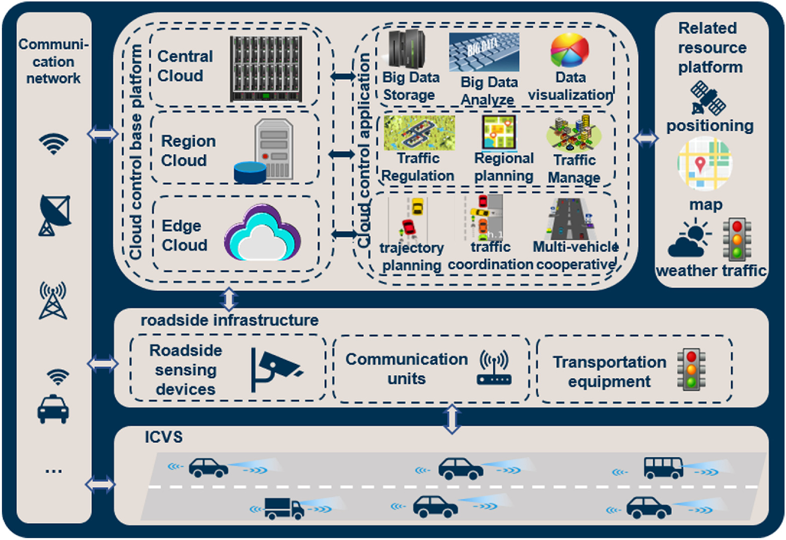
Placing the vehicle platoon under CCS can further amplify its advantages. The predictive algorithm is deployed on the edge cloud, calling on road information ahead of the drive based on the vehicle’s current location to quickly calculate optimal running speed. The regional cloud can predict traffic dynamics in the region and provide support for PPCC. The central cloud is used for non-real-time data analysis of the vehicle platoon operation, platoon energy consumption statistics, and the like.
CPPCC Layered Architecture
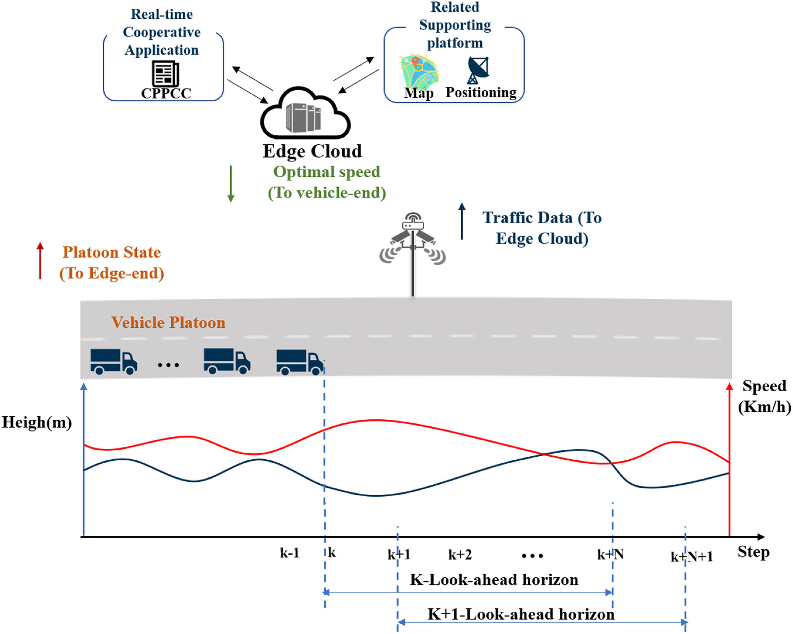
The CPPCC system architecture is shown in Fig. 2. Cloud deployment includes both static (geometric) road information and dynamic traffic information (real-time traffic flow mapping and dynamic traffic flow) in its underlying platform The problem of platoon longitudinal speed optimization based on static road information is prioritized in this paper. The application platform of the edge cloud deploys a cloud-based predictive cruising speed optimization algorithm. The support platform provides vehicle-positioning and road slope information ahead of driving as data support. The cloud predicts the optimized speed and gear sequence and sends the information down to the vehicle controller of the platoon. The controller parses the gear and speed sequences and outputs the optimal control volume.
PPCC studies of homogenous platoons use the state of the leader vehicle as the inverse feedback for speed planning (Zhai et al. 2020). Here, the slope of the road in cloud-based speed planning is divided by a length of 200 m. The length of the entire platoon is less than 200 m and the slope is essentially less variable within that range. The maximum slope of the highway is no more than 5%, which can be idealized as approximately the same throughout the range of the vehicle platoon. Assuming that the state of the platoon is stable at the moment of optimization, the vehicle state of the platoon vehicles can be approximately the same at this time. Thus, we can use the leader car information as the vehicle platoon’s state information real-time feedback to the cloud. The difficulty of system design and algorithm computation time can be greatly reduced by this assumption.
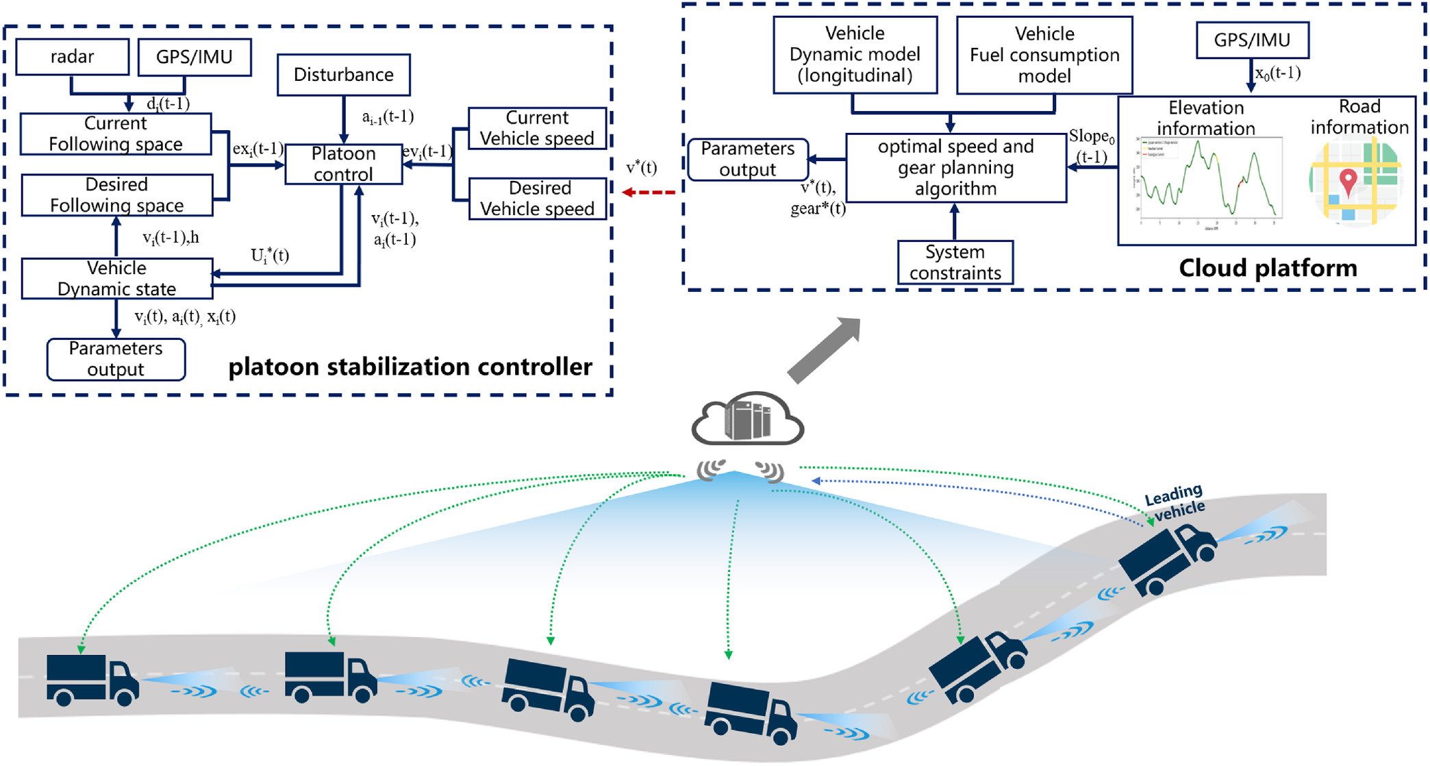
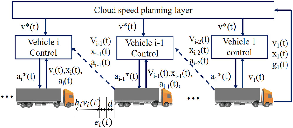
The overall framework for the CPPCC information flow is shown in Fig. 3. CPPCC uses the vehicle platoon’s leader car information as the platoon’s state information real-time feedback to the cloud. The cloud, according to the leader car feedback, first targets speed information and location information, through the map positioning module, to determine vehicle platoon state ahead of road elevation information. The static road slope information and the leader vehicle feedback state (speed, position, and gear) information as the cloud-based speed planning layer’s information. This determines the optimal speed and gear sequence through the predictive cruise algorithms and sends it to all vehicles in the platoon. The following vehicles calculate their desired acceleration according to the speed and gear sequence sent from the cloud. The error in spacing with the previous vehicle in the platoon, the acceleration of the previous vehicle, and the vehicle state information (speed, position, acceleration) are taken as input to the platoon’s stability controller.
CPPCC Communication Topology
The traditional topology of vehicle platoon communication is mainly predecessor-following (PF), predecessor-leader–following (PLF), two-predecessor–following (TPF), and two-predecessor-leader–following (TPLF) (Li et al. 2015). However, when combined with the cloud platform, the communication topology needs to take into account the practical needs and applications of vehicle platoons and cloud communication. We add cloud nodes to the traditional vehicle platoon, change the traditional communication topology, and propose a CPPCC communication topology. We weaken the role of the leader vehicle, considering it as the vehicle node in the platoon, and add the cloud as a node to implement the CPPCC topology.
The topology can be modeled using a directed graph (Zheng et al. 2017; Li et al. 2015), where , are the individual connected nodes and the cloud is defined as node 0.
The adjacency matrix A describes the flow of information between vehicles, where is an element in A; means that vehicle () has access to the state information of vehicle but vehicle does not have access to the state information of vehicle
(1)
Vehicle can obtain the status of the remaining vehicles in the vehicle platoon as . The matrix expresses the cloud communication and the connectivity of the vehicles in the platoon, emphasizing the role of the cloud as a communication node in the platoon compared with traditional communication. The cloud and vehicle platoon matrix are defined as . If , the vehicles and the cloud communicate with each other; otherwise, there is no communication. The communication settings of the cloud and vehicle can be characterized as in Eq. (2)
(2)
The communication topology of CPPCC is thus expressed as in Eq. (3)
(3)
Cloud Speed Planning Algorithm
Rolling optimization-based platoon speed planning for cloud deployment has the objective of reducing fuel consumption and total running time. The optimization problem is solved in a discrete space using a vehicle longitudinal dynamics model, a fuel consumption model, and receding dynamic programming (RDP).
Longitudinal Dynamics Model
The longitudinal dynamics of the vehicle are modeled to consider vehicle dynamics, wind resistance, roll resistance, and ramp resistance. Due to the mass and dynamics of commercial vehicles, the algorithm focuses on the effect of road slope on longitudinal dynamics and thus considers speed optimization in the optimization process.
The following is based on a nonlinear longitudinal vehicle dynamics model, which is based on the single-wheeled vehicle model presented, assuming that forces act equally on the wheels. The main driving force for the vehicle to move forward comes from friction on the ground. The main factors affecting the longitudinal force on the tires are longitudinal speed of the vehicle and equivalent speed of the tire. The speed of the tire is obtained from the torque generated by the combustion of the engine fuel through a series of transmission transformations such as torque conversion and transmission. The dynamic model of the engine can be described using the following equation:where = rotational inertia of the engine; = engine speed; = net engine torque; and = torque that the engine transfers to the clutch when it is put into gear. The turbine is connected to the transmission and causes the transmission to rotate at the same speed as the turbine, thus driving the car. When the torque converter is in lock-up, the pump torque is equal to the turbine torque
(4)
(5)
The vehicle is equipped with an automatic transmission, which operates by a combination of hydraulic transmission and gearing to achieve variable torque. Assuming that the transmission is in a steady state of operation without gear changes, let the gear ratio be ; then the dynamic model of the transmission can be expressed as
(6)
(7)
At this point, for the drive wheels of the car, the dynamics of its rotation are modeled as
(8)
This assumes that the torque converter is locked and the transmission is working in a stable state of gear, ignoring the slippage of the tire. The wheel speed is proportional to the engine speed , and the ratio is the gear ratio as . The driveshaft speed is the same as the engine speed . At this time the longitudinal acceleration of the vehicle is
(9)
The longitudinal dynamics of the vehicle are analyzed as shown in Fig. 4, and the longitudinal forces on the vehicle are analyzed for vehicle aswhere = speed of the vehicle; = mass of vehicle; and = engine traction force. The force provided by the engine and transmitted to the tire via the transmission.
(10)
(11)
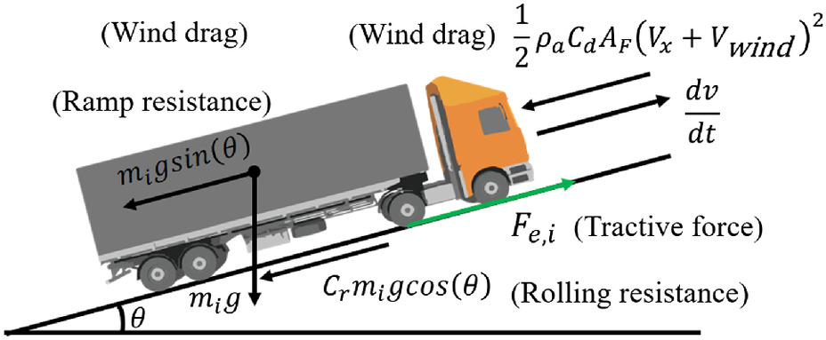
is the resistance to slope and vehicle is driving on a road with an inclination angle of . The resistance to a slope of the vehicle at this point iswhere = mass of vehicle ; = acceleration of gravity; and = rolling resistance asand = rolling resistance coefficient. The air resistance during vehicle operation iswhere = air density; = air drag coefficient; = frontal wind area of the vehicle; and = wind speed.
(12)
(13)
(14)
The driving force of the vehicle at this point can be expressed as
(15)
The tire torque required to produce the desired acceleration at this point is
(17)
Combining Eqs. (4)–(17), the relationship between the net vehicle torque and the desired acceleration can be obtained as
(18)
The specific parameters of the vehicle are shown in Table 1.
| Parameter | Symbol | Value |
|---|---|---|
| Engine | ||
| Engine speed range () | [750 3250] | |
| Engine torque range (Nm) | [25 375] | |
| Moment of inertia () | [2.5 3.5] | |
| Driveline | ||
| Final drive ratio | 5 | |
| Transmission ratio | [5.9 3.365 2.129 1.518 1.0 0.783] | |
| Final drive efficiency | 0.92 | |
| Transmission efficiency | [0.55, 6.8, 0.92, 9.81, 1.206, 0.459] | |
| Longitudinal force | ||
| Vehicle curb mass (kg) | 6,500 | |
| Effective tire radius (m) | 0.459 | |
| Frontal area () | 6.8 | |
| Air drag coefficient | 0.55 | |
| Rolling resistance coefficient | [0.010 0.018] | |
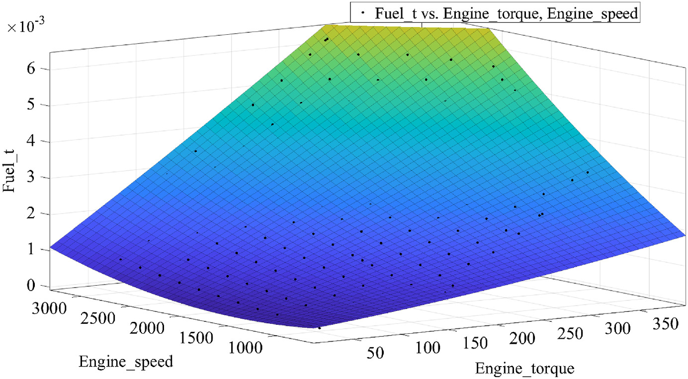
Engine Fuel Consumption Model
According to the generic characteristics of a commercial vehicle model, a fuel consumption model of the engine is established. A high-fidelity polynomial model of engine fuel consumption is fitted according to linear interpolation and polynomial fitting as shown in Fig. 5. The model is a quadratic polynomial function of vehicle speed and engine torque as shown in Eq. (19)where = fit coefficient.
(19)
Receding Dynamic Programming Algorithm
Receding distance domain optimization involves predicting the future state of the system and static road slope information. To resist external disturbances and prediction uncertainties, model prediction is used to offset the uncertain perturbations of the system by rolling distance domain optimization. The optimization is accomplished by RDP as shown in Fig. 6, where the foreseeability region for each plan is (part of the total mileage of the run) divided into stages according to the same. The optimization is performed by solving backward from Post-stage to Stage 1 within the optimized foreseeability region. After completion of the solution, the optimal solution for Stage 1 is applied to PCC in the current time cycle. Because of the uncertainty of the future state of the remaining stages, only the optimal solution for Stage 1 is used and the action is repeated at the beginning of the next cycle.
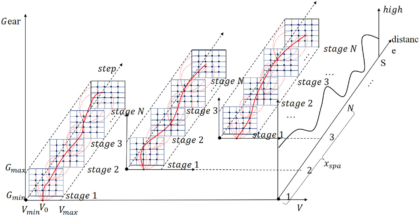
RDP needs to decompose one optimization problem into several subproblems to solve it. In space, the speed optimization problem is divided into each stage to be solved separately. The algorithm’s single optimization distance is . The single planning interval point is divided into stages, while the length of the spacing division within a stage is . Using the maximum and minimum velocities planned by the algorithm as intervals, the velocity interval is set as and the velocity states of the planning are distinguished into states to establish the state space of the algorithm planning. In this paper, considering the effectiveness of the algorithm to solve the speed and planning speed, we set the distance of a single optimization to the area of 2 km in front of the vehicle running and set as the planning stage, which divides one planning stage into stages. The gear setting affects driving performance, which in turn has a great impact on fuel performance. Therefore, RDP needs to consider its optimization. The transfer functions for the two-state points are as in Eq. (20)where = cost function of the state point to the next state; and = cost of the next state to the final state, ensuring that the state point to the final state is also optimal.
(20)
(21)
Construction of Cost Functions for Receding Dynamic Programming
According to Eq. (22), the cost function of the state point to the next state point is . The optimization objectives of the function are to reduce energy consumption and prevent deviations from the set reference speed, speed fluctuations, and frequent gear changeswhere = penalty factor for the running fuel consumption optimization term, which ensures the fuel economy of the vehicle during driving; = penalty factor for the optimization term of the deviation of the planned speed from the reference speed, which prevents the planned speed deviating too much from the set reference speed; and = penalty factor for the speed variation between states for avoiding large speed fluctuations. Gear variation is a penalty factor for the fourth term of Eq. (22) for avoiding a large range of gear variations.
(22)
Solving Process for Receding Dynamic Programming
Following is the cloud-based speed planning algorithm:
| 1. Divide state space into phases of the plan with , . The state is divided within the velocity interval of the plan with , as . The velocity state interval of the next phase is also divided as . |
| 2. Set , , , , and calculate the system cost function for the transition from the th state to state when the block is . Add the state to the final state to obtain the final cost of the transfer . |
| 3. If , the initial cost is stored in the cost function matrix , the optimal speed is stored in , and the optimal gearbox transmission is stored in ; if , update the cost function. |
| 4. g = g + 1; if , back to Steps 2 and 3. |
| 5. j = j + 1; if , back to Steps 2, 3, and 4. |
| 6. ; if , back to Steps 2, 3, 4, and 5. |
| 7. Starting from the initial state , the optimal sequence of speeds and optimal gears is solved forward according to the stored optimal speed matrix and optimal gears . |
| 8. Platoon optimization speed for the first stage of cloud-down solving after interpolation densification. |
Cooperative Platoon Stabilization Control
After an optimized speed sequence is sent from the cloud, the speed-tracking control layer’s distributed controller ensures the stability of the entire platoon while tracking the speed from the cloud. The vehicle side carries a DMPC to track the speed sent from the cloud and to ensure the previous vehicle’s following distance. Platoon stability control framework is shown in Fig. 7, we treat the platoon as composed of homogeneous vehicles. The variables , , and denote the position, velocity, and acceleration of vehicle (, when the vehicle is the leader vehicle). The spacing of the vehicles is set as constant time headway (CTH).
This section is concerned with the DMPC in the vehicle control layer. Vehicle receives the optimal speed sent down from the cloud and obtains the state information of the vehicle in front of it. By tracking optimal speed and spacing, optimal control sequences are generated by tracking the optimal speed profile and vehicle spacing requirements while satisfying safety constraints. Before performing the DMPC derivation, we assume that (1) the body is rigid and symmetrical from side to side, (2) the vehicle is driven on a flat, dry asphalt surface where the longitudinal slip of the wheels is neglected, and (3) the drive and brake torques are integrated into a single control input.
The derivation of DMPC, which includes the vehicle model, the vehicle system constraint limits, safety constraints, and the cost function of the system, is presented next.
Analysis of Platoon System Dynamics
The longitudinal control of the platoon belongs to the tracking control of the vehicles. The main objective is to track the optimal speed sent down from the cloud and adjust the spacing of the platoon according to the set spacing strategy. In this study, the spacing strategy is set aswhere = set desired vehicle spacing for the platoon; = predefined constant time distance factor; and = set safe spacing when the vehicle is stopped. Then the vehicle travels with the set spacing strategy error and speed tracking error aswhere = position of the vehicle at .
(23)
(24)
(25)
Time lags in the drive need to be considered in vehicle dynamics, rather than assumed to be instantaneous realization of acceleration, as the vehicle system needs a certain amount of time to achieve the required accelerationwhere = acceleration of the vehicle; = vehicle control input, which is the desired acceleration of the vehicle; and = drive time lag of the vehicle. At this point we define the state of the system (Zhai et al. 2019a; Zhou et al. 2019)where = state of the system; = control input; and = disturbance input.
(26)
(27)
(28)
Although the dynamics of the vehicle is continuous, it needs to be discretized during the solution process. A discrete version of the state space can be obtained by assuming that the control inputs are zero-order keepers (Rakovic et al. 2005)
(29)
(30)
(31)
(32)
A system dynamics model based on the system’s current state and the predicted future state solves the optimal control problem at each time step of the prediction horizon . The controller implements only the first control input (i.e., the optimal solution at time step ) and recalculates the optimal control over the prediction horizon starting at the next time step .
The optimal control sequence (the acceleration specified by the controller), the predicted future state of the optimal control, and the actual realized state with unmodeled and unknown disturbances, , denotes the optimal control sequence of the vehicle from the predicted range ; denotes the desired condition of the vehicle from to the predicted range ; denotes the actual state of the vehicle from to the predicted range , where is the vehicle control initial state. Based on the above model, the solution algorithm for the DMPC will be developed in the following sections.
Platoon Optimal Control Problem Construction
Under the condition of no collision constraint and vehicle acceleration constraint, optimal control is established by considering vehicle tracking control accuracy and driving comfort. According to the goal of optimal control, the cost function is set aswhere = prediction range; = cost of each stage of the system before reaching equilibrium; = terminal cost of the end state to the desired point; = initial condition constraint equal to the measured state at ; = state that adjusts the cost of the maximum deviation from the desired output or acceleration constraint at each time point; = acceleration constraint to ensure that the control quantity is within a reasonable range of , where and represent the upper and lower limits of acceleration, respectively; and = terminal state constraint, which is used to adjust the terminal state toward the desired terminal state.
(33)
For the derivation of optimal control, the stage and terminal costs are specified, thereby deriving local stability and global string stability, which includes a stage cost function aswhere = desired output of a positive definite state matrix as in Eq. (35); and = weight considering comfort, which is constantly greater than 0
(34)
(35)
The end-state cost is , where is used as a solution to the discrete algebraic Recatti equation (DARE; Rakovic et al. 2005) to ensure local stability. The expression at this point is
(36)
Platoon System Constraints
The platoon stabilization controller needs to satisfy the following constraints.
1.
Safety constraint: the safety constraint is a requirement to avoid collisions between vehicles in the platoon and the vehicle in front, which includes a range of errors in the platoon’s vehicle distance
(37)
2.
Performance requirements: the platoon’s safety and stability are important in ensuring that the entire platoon travels at an identical speed. In the process of system operation, the vehicles’ speed error is
(38)
3.
Desired speed interval: combined with the realistic situation of the highway speed constraint interval, set the constraint to ensure that platoon operating speed is in line with the reality of the situation
(39)
4.
Comfort: comfort is an important indicator of the smoothness of the control; the acceleration and deceleration rate in the controlled acceleration interval should satisfy the comfort interval
(40)
5.
Actuator limits: due to the physical limitations of a real vehicle, the amount of control given by the controller (desired acceleration) must be within the range that the vehicle actuator can perform
(41)
6.
Stability requirements: when the platoon is in operation, it normally uses the spacing error to define stability. It means that the spacing error will not be enlarged step by step with the platoon and can converge to ensure stability of the whole platoon, which is satisfied as
(42)
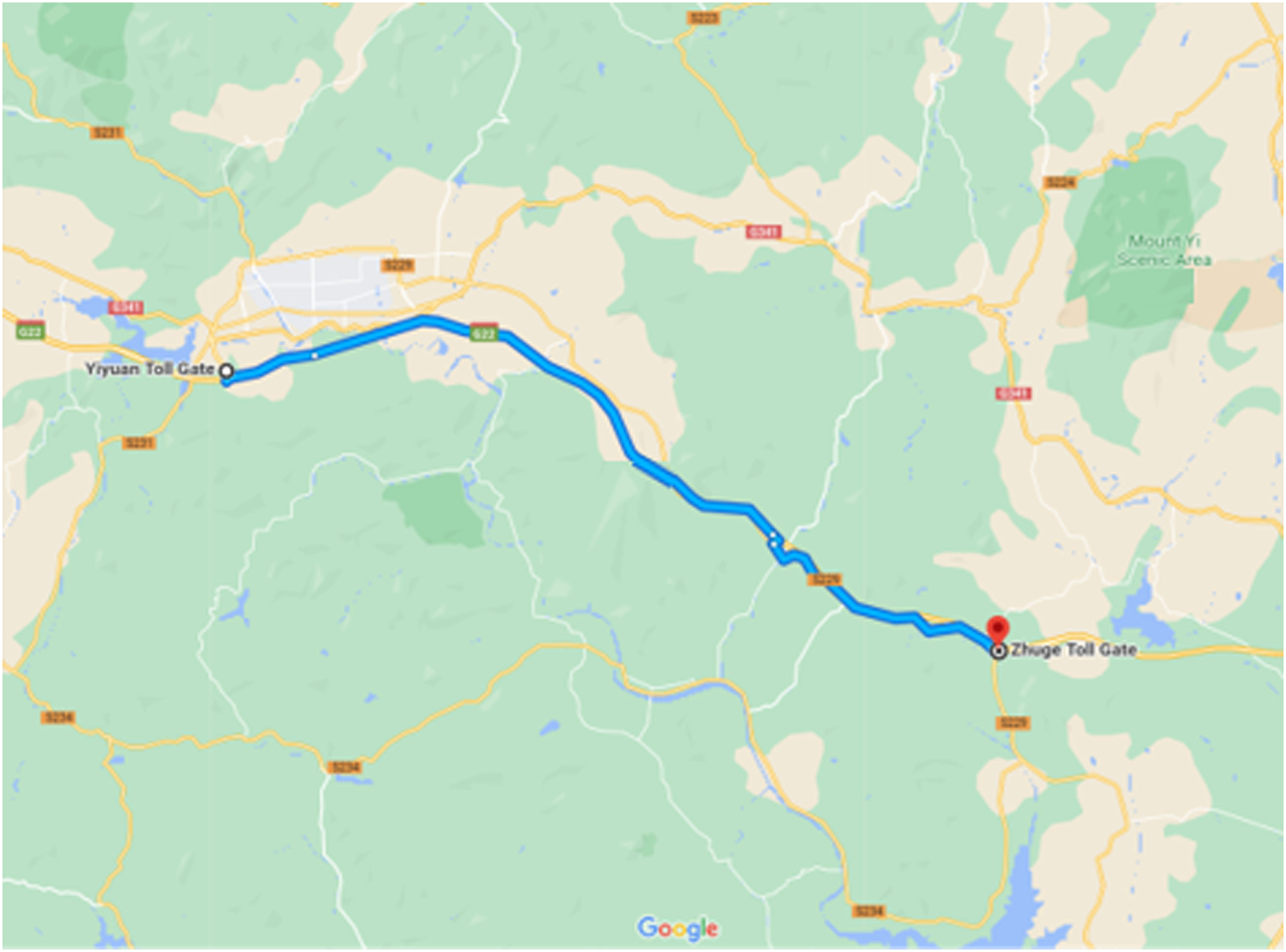
Simulation Experiments and Analysis
To verify the effectiveness of CPPCC, we built simulation experiments based on Trucksim and Matlab/Simulink. The simulation experiments were carried out on the Yi yuan-Zhu ge section of the G22 highway in Shandong Province as shown in Fig. 8. The real vehicle was selected from a real vehicle factory, and the vehicle parameters included the basic parameters of the vehicle and the engine model.
Simulation Experiment Setup
To verify the effectiveness of the proposed method, a comparison experiment was set up to validate the experimental platoon of six commercial vehicles. The metrics of interest were total vehicle platoon run time, total fuel consumption, and spacing and speed stability metrics. The comparison scenarios were set up and the CPPCC methods were compared.
1.
Cruise control (CC): fixed-gear PLF-cruise control platoon (PLF-CC) and PF-cruise control platoon (PF-CC) in conventional communication topology. PLF-CC and PF-CC used the same DMPC controller as in CPPCC.
2.
CPPCC: The predictive cruise control algorithm considering road slope was deployed in the cloud and the vehicle platoon was equipped with a platoon stabilization controller.
The spacing policy of the vehicle platoon was set CTH and ensured a safe stopping distance of 5 m between vehicles to protect the safety of the whole platoon.
The simulation experiments used automatic transmission, but there is frequent gear shifting in the road section, which leads to high fuel consumption in the whole road, so the PLF-CC and PF-CC platoon with six fixed gears was chosen.
Simulation of the Experiment
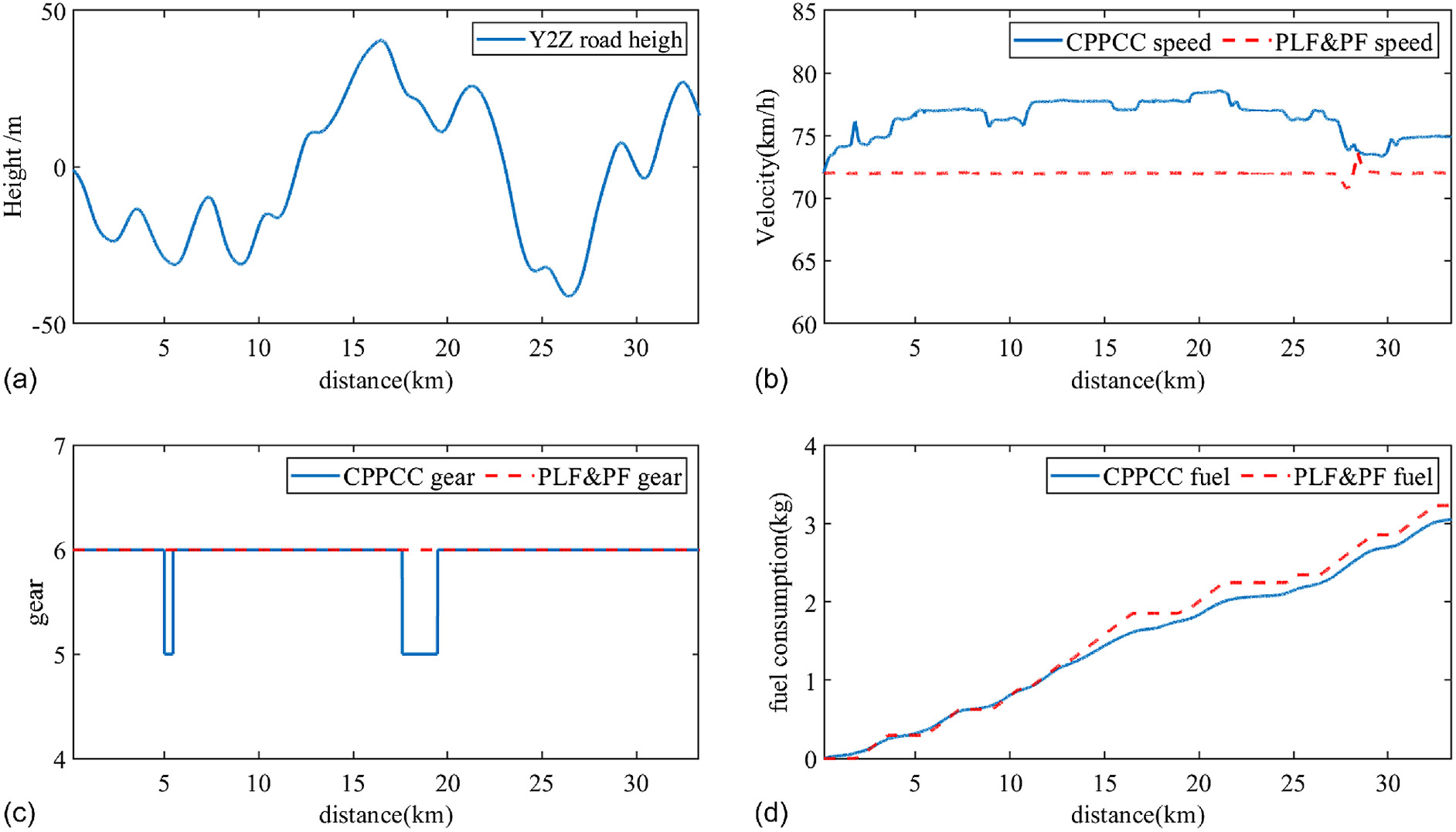
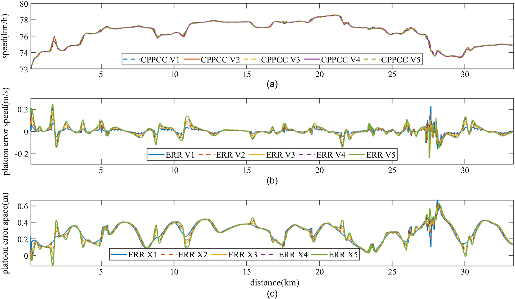
The energy consumption and platoon control effects of CPPCC for the entire test section are illustrated. The results of the experiments for CPPCC over the entire length are shown in Fig. 9, while Fig. 10 shows the effect of platoon stability control over the entire length. CPPCC speed was higher than PLF-CC and PF-CC speed throughout the entire route. The fuel consumption of each vehicle in the platoon is shown in Table 2. It can be seen that CPPCC saved 5.13% and 5.94% of energy compared with traditional PF-CC and PLF-CC in the cloud-based communication topology. CPPCC made the whole platoon more efficient and consumed the least amount of energy. Experimental statistics on speed errors and space errors in vehicle platoon stability control are shown in Tables 3 and 4. The speed error of the platoon remained within [, 0.30] () and the spacing error was guaranteed to be within [, 0.66] (m) throughout the process. CPPCC safely achieved efficient and energy-saving operation of the entire vehicle platoon.
| Type | Consumption (kg) | Time (s) | Fuel increase rate (%) | ||||||
|---|---|---|---|---|---|---|---|---|---|
| Sum | |||||||||
| PF-CC | 3.233 | 3.263 | 3.275 | 3.281 | 3.295 | 3.310 | 19.657 | 1,660.7 | 5.94 |
| PLF-CC | 3.233 | 3.242 | 3.243 | 3.244 | 3.245 | 3.283 | 19.489 | 1,660.7 | 5.13 |
| CPPCC | 3.076 | 3.073 | 3.073 | 3.074 | 3.075 | 3.118 | 18.490 | 1,565.9 | — |
| Err_speed () | Range | Aver | A1 | A2 | A3 | A4 | A5 |
|---|---|---|---|---|---|---|---|
| Err_v1 | [, 0.228] | 0.002 | 0.006 | 0.431 | 0.559 | 0.003 | 0.001 |
| Err_v2 | [, 0.217] | 0.003 | 0.007 | 0.447 | 0.539 | 0.007 | 0 |
| Err_v3 | [, 0.272] | 0.004 | 0.011 | 0.456 | 0.523 | 0.010 | 0 |
| Err_v4 | [, 0.280] | 0.004 | 0.018 | 0.465 | 0.493 | 0.022 | 0.002 |
| Err_v5 | [, 0.260] | 0.005 | 0.024 | 0.470 | 0.470 | 0.033 | 0.004 |
Note: A1: []; A2: []; A3: [0,0.1]; A4: [0.1,0.2]; and A5: [0.2,0.3].
| Err_space (m) | Range | Aver | B1 | B2 | B3 | B4 | B5 |
|---|---|---|---|---|---|---|---|
| Err_x1 | [0, 0.670] | 0.277 | 0 | 0.277 | 0.627 | 0.094 | 0.002 |
| Err_x2 | [, 0.636] | 0.276 | 0.001 | 0.278 | 0.626 | 0.095 | 0.002 |
| Err_x3 | [, 0.614] | 0.275 | 0.002 | 0.287 | 0.606 | 0.102 | 0.003 |
| Err_x4 | [, 0.631] | 0.275 | 0.010 | 0.284 | 0.592 | 0.111 | 0.004 |
| Err_x5 | [, 0.637] | 0.274 | 0.016 | 0.287 | 0.564 | 0.127 | 0.005 |
Note: B1: [, 0]; B2: [0,0.2]; B3: [0.2,0.4]; B4: [0.4,0.6]; and B5: [0.6,0.8].
Analysis in Different Simulation Sections
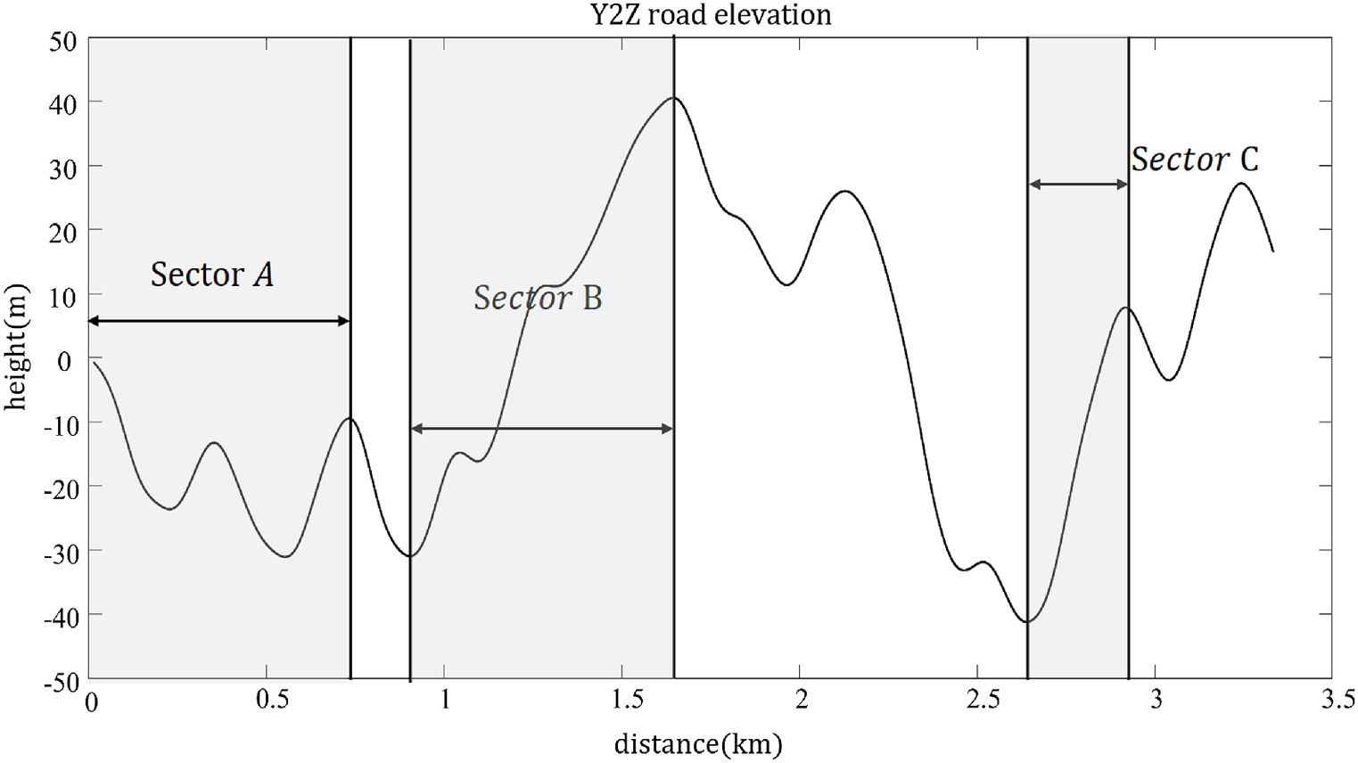
According to its characteristics, we divided the experimental road section into three parts as shown in Fig. 11 for analysis of effectiveness. Section A was a continuous slope with continual changes in slope. Section B was a long uphill section with short-distance downhill sections. Section C was an uphill section. CPPCC control effectiveness at different slope variations was verified.
The operation of the leader vehicle in the vehicle platoon in Section A was analyzed first. Section A had continual slope changes. The energy-saving effect of the CPPCC and its overall control of the platoon are illustrated in Fig. 12. CPPCC adapted to changes in road slope by adjusting the cruising speed at any time. The optimum gear for most of the time throughout was the sixth gear, with a drop to 5th gear midway through to avoid excessive speed when downshifting to use engine braking going downhill. Fuel consumption in Section A was slightly lower compared with PLF-CC and PF-CC, where energy consumption was 0.6214 and 0.6016 kg, respectively. Analysis of the fuel consumption curve shows that, CPPCC was faster going downhill and corresponding fuel consumption was higher. But greater speed enabled the vehicle to charge the uphill, so that the torque of the engine was not too high, thus causing a reduction in fuel consumption and saving 3.19% fuel consumption. Under the control of DMPC, the speed error of the platoon was between [, 0.242] () and the spacing error was [, 0.45] (m). The platoon showed more stable spacing and speed.
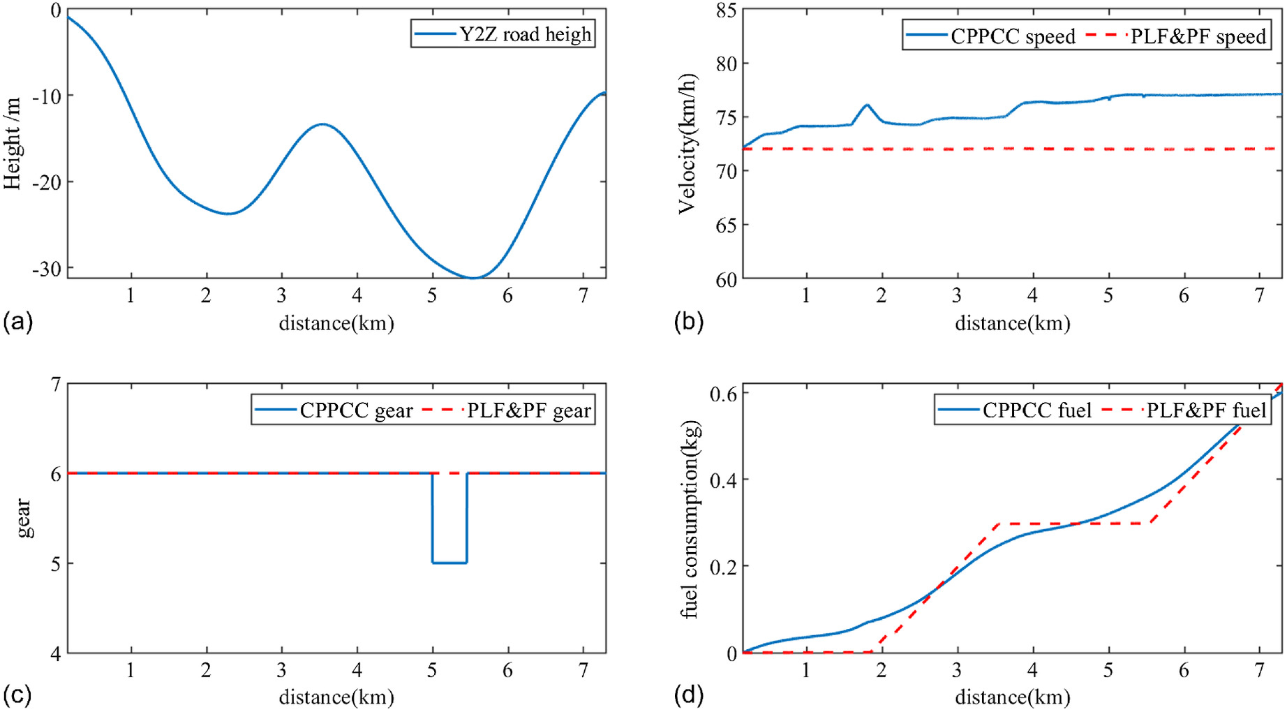
At the same distance, the efficiency of CPPCC improved by 5.70% compared with PLF-CC and PF-CC in ensuring a stable platoon and fuel consumption savings of 3.19%.
Section B was a continuous uphill section. Fig. 13 shows the results of the simulation of this section. CPPCC adjusted the vehicle to go uphill at a higher speed according to the road slope and ensured a constant speed on the road section to reduce fluctuations. The fuel consumption of the PLF-CC and PF-CC leader in the section was 1.224 kg, while the fuel consumption of the CPPCC leader vehicle was 0.939 kg. The energy-saving effect of this continuous uphill section was very obvious, with a saving ratio of 23.3%. Under the control of DMPC, the speed error was [, 0.139] () and the spacing error was [0.063,0.458] (m).
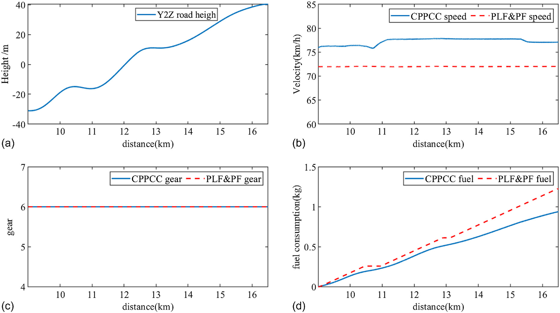
At the same distance, the efficiency of CPPCC was improved by 6.77% compared with PLF-CC and PF-CC with guaranteed platoon stability, and there was a significant improvement in energy saving of 23.3%.
Section C was an uphill section. In Fig. 14, the results of its simulation are shown. CPPCC ensured that the vehicle speed was controlled at a higher speed and that the optimal gear was the sixth gear throughout. The energy consumption of the PLF-CC and PF-CC leader was 0.3973 kg, while the energy consumption of the CPPCC leader was 0.3546 kg. Moreover, the running time on this same section was reduced by 3.18%. The speed error was [, 0.225] () and the spacing error was [0.100,0.668] (m) under DMPC control.
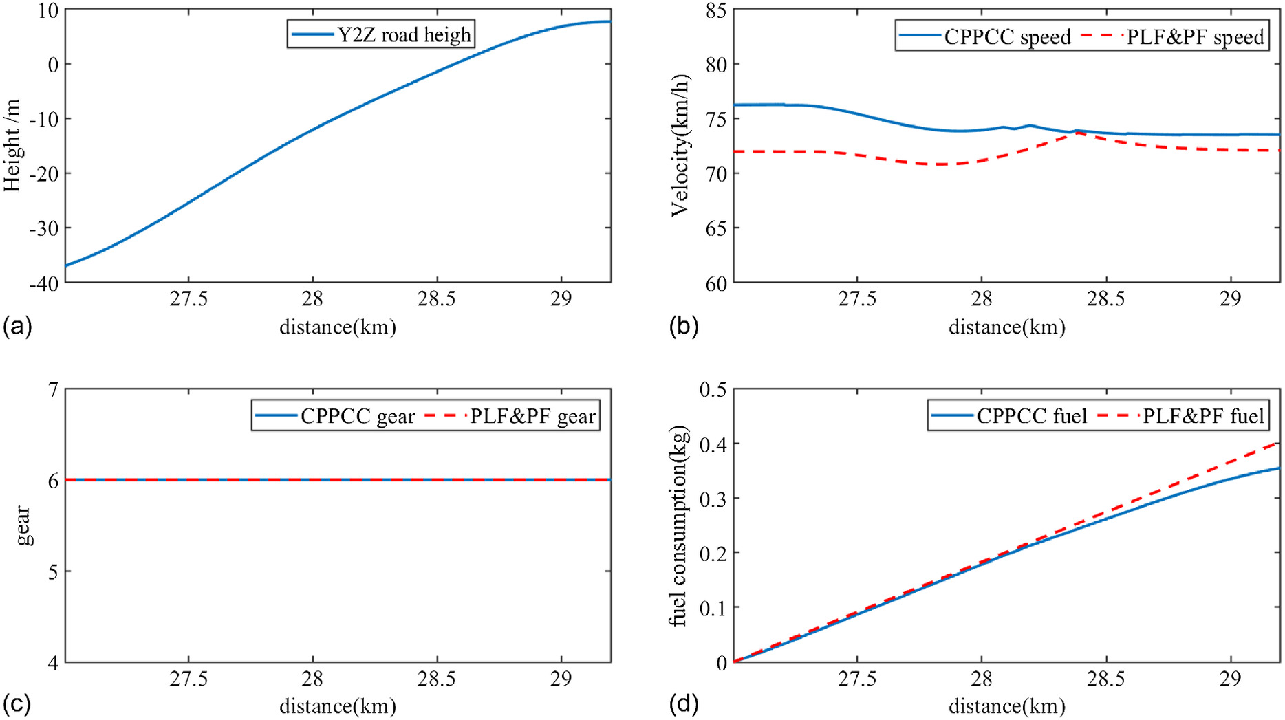
At the same distance, the efficiency of CPPCC was improved by 3.18% compared with PLF-CC and PF-CC with guaranteed platoon stability. There was also a significant improvement in energy saving, of 10.75% on this section.
Conclusions
This paper proposed a hierarchical CPPCC approach based on the CCS. The hierarchical control architecture and communication topology of CPPCC was proposed to implement the deployment of a PCC algorithm based on road slope information in the cloud and DMPC on the vehicle side. Coupling control of PPCC and platoon stability control based on road slope in the cloud was developed. The cloud-based PCC algorithm addressed energy efficiency, enabling economical and efficient driving in the entire platoon. DMPC on the vehicle side calculated the recommended speed command issued by the cloud and guaranteed the stability of the platoon while ensuring tracking accuracy. A comprehensive solution to PPCC safety, energy saving, and efficiency was achieved. Simulation experiments with real road and vehicle data models compared the method proposed in this paper with traditional PLF-CC and PF-CC. The speed error remained within [, 0.30] () and the spacing error was guaranteed to be within [, 0.66] (m). The fuel saving was more than 5.13%, and overall operating efficiency was improved by 5.71%, which proves the effectiveness of the method. CPPCC is decoupled from hierarchical in this paper. It tackles the problem of platoon stability, while the cloud focuses on traffic efficiency and energy consumption.
To highlight the effectiveness of CPPCC, the effect of operating in more ideal conditions without interfering with vehicles in front was assumed. In the future, with the advantages of roadside sensing, in-vehicle sensing, and cloud-based information fusion, the results of forward over-the-horizon obstacle sensing and dynamic traffic flow information will be taken into account. Using these results, the issues of energy efficiency and stable tracking of an integrated platoon in the cloud can be achieved. As for commercial vehicle platoons, the impact of actuator hysteresis on overall control is huge. For this reason, the problem of vehicle actuator hysteresis needs to be considered in CPPCC.
Data Availability Statement
Some or all data, models, or code that support the findings of this study are available from the corresponding author upon reasonable request.
Acknowledgments
This work was supported by the National Key Research and Development Program (2021YFB2501000), and the R&D Project on Key Technologies for Intelligent connected Vehicles based on Modular computing base platform (20202000342).
References
Bakibillah, A. S. M., M. A. S. Kamal, C. P. Tan, T. Hayakawa, and J. Imura. 2018. “Eco-driving on hilly roads using model predictive control.” In Proc., Joint 7th Int. Conf. on Informatics, Electronics & Vision (ICIEV) and 2018 2nd Int. Conf. on Imaging, 20–22. New York: IEEE.
Guo, G., and Q. Wang. 2019. “Fuel-efficient en route speed planning and tracking control of truck platoons.” IEEE Trans. Intell. Transp. Syst. 20 (8): 3091–3103. https://doi.org/10.1109/TITS.2018.2872607.
Guo, X., J. Wang, F. Liao, and R. S. H. Teo. 2017. “Distributed adaptive sliding mode control strategy for vehicle-following systems with nonlinear acceleration uncertainties.” IEEE Trans. Veh. Technol. 66 (2): 981–991. https://doi.org/10.1109/TVT.2016.2556938.
Kamal, M. A. S., M. Mukai, J. Murata, and T. Kawabe. 2011. “Ecological vehicle control on roads with up-down slopes.” IEEE Trans. Intell. Transp. Syst. 12 (3): 783–794. https://doi.org/10.1109/TITS.2011.2112648.
Kazemi, H., H. N. Mahjoub, A. T. Sarvestani, and Y. P. Fallah. 2018. “A learning-based stochastic MPC design for cooperative adaptive cruise control to handle interfering vehicles.” IEEE Trans. Intell. Veh. 3(3): 266–275. https://doi.org/10.1109/TIV.2018.2843135.
Li, K., X. Chang, J. Li, Q. Xu, B. Gao, and J. Pan. 2020a. “Cloud control system for intelligent and connected vehicles and its application.” Automot. Eng. 42 (12): 1595–1605. https://doi.org/10.19562/j.chinasae.qcgc.2020.12.001.
Li, K., J. Li, X. Chang, B. Gao, Q. Xu, and S. B. Li. 2020b. “Principle and typical application of cloud control system for intelligent networked vehicles.” J. Automot. Saf. Energy Conserv. 11 (3): 261–275. https://doi.org/10.3969/j.issn.16748484.2020.03.001.
Li, S., K. Wan, B. Gao, R. Li, Y. Wang, and K. Li. 2022. “Predictive cruise control for heavy trucks based on slope information under cloud control system.” J. Syst. Eng. Electron. 33 (4): 812–826. https://doi.org/10.23919/JSEE.2022.000081.
Li, S. E., Y. Zheng, K. Li, and J. Wang. 2015. “An overview of vehicular platoon control under the four-component framework.” In Proc., 2015 IEEE Intelligent Vehicles Symp. (IV) Conf., 286–291. New York: IEEE.
Maged, M., D. M. Mahfouz, O. M. Shehata, and E. I. Morgan. 2020. “Behavioral assessment of an optimized multi-vehicle platoon formation control for efficient fuel consumption.” In Proc., 2nd Novel Intelligent and Leading Emerging Sciences Conf., 24–26. New York: IEEE.
Ozatay, E., S. Onori, J. Wollaeger, U. Ozguner, G. Filev, D. Rizzoni, J. Michelini, and S. D. Cairano. 2014. “Cloud-based velocity profile optimization for everyday driving: A dynamic-programming-based solution.” IEEE Trans. Intell. Transp. Syst. 15 (6): 2491–2505. https://doi.org/10.1109/TITS.2014.2319812.
Rakovic, S. V., E. C. Kerrigan, K. I. Kouramas, and D. Q. Mayne. 2005. “Invariant approximations of the minimal robust positively invariant set.” IEEE Trans. Autom. Control 50 (3): 406–410. https://doi.org/10.1109/TAC.2005.843854.
Turri, V., B. Besselink, and K. H. Johansson. 2017. “Cooperative look-ahead control for fuel-efficient and safe heavy-duty vehicle platooning.” IEEE Trans. Control Syst. Technol. 25 (1): 12–28. https://doi.org/10.1109/TCST.2016.2542044.
Wu, Y., S. E. Li, J. Cortes, and K. Poola. 2020. “Distributed sliding mode control for nonlinear heterogeneous platoon systems with positive definite topologies.” IEEE Trans. Control Syst. Technol. 28 (4): 1272–1283. https://doi.org/10.1109/TCST.2019.2908146.
Yang, Y., F. Ma, J. Wang, S. Zhu, and L. Guvenc. 2020. “Cooperative ecological cruising using hierarchical control strategy with optimal sustainable performance for connected automated vehicles on varying road conditions.” J. Cleaner Prod. 275 (1): 123–136. https://doi.org/10.1016/j.jclepro.2020.123056.
Yu, K., H. Yang, X. Tan, T. Kawabe, Y. Guo, Q. Liang, Z. Fu, and Z. Zheng. 2016. “Model predictive control for hybrid electric vehicle platooning using slope information.” IEEE Trans. Intell. Transp. Syst. 17 (7): 1894–1909. https://doi.org/10.1109/TITS.2015.2513766.
Yu, X., G. Guo, and H. Lei. 2018. “Longitudinal cooperative control for a bidirectional platoon of vehicles with constant time headway policy.” In Proc., Chinese Control and Decision Conf. (CCDC), 2427–2432. New York: IEEE.
Zhai, C., X. Chen, C. Yan, Y. Liu, and H. Li. 2020. “Ecological cooperative adaptive cruise control for a heterogeneous platoon of heavy-duty vehicles with time delays.” IEEE Access 8 (99): 146208–146219. https://doi.org/10.1109/ACCESS.2020.3015052.
Zhai, C., Y. Liu, and L. Fei. 2019a. “A switched control strategy of heterogeneous vehicle platoon for multiple objectives with state constraints.” IEEE Trans. Intell. Transp. Syst. 20 (5): 1883–1896. https://doi.org/10.1109/TITS.2018.2841980.
Zhai, C., F. Luo, Y. Liu, and Z. Chen. 2019b. “Ecological cooperative look-ahead control for automated vehicles travelling on freeways with varying slopes.” IEEE Trans. Veh. Technol. 68 (2): 1208–1221. https://doi.org/10.1109/TVT.2018.2886221.
Zheng, Y., S. E. Li, K. Li, F. Borrelli, and J. K. Hedrick. 2017. “Distributed model predictive control for heterogeneous vehicle platoons under unidirectional topologies.” IEEE Trans. Control Syst. Technol. 25 (3): 899–910. https://doi.org/10.1109/TCST.2016.2594588.
Zhou, Y., M. Wang, and S. Ahn. 2019. “Distributed model predictive control approach for cooperative car-following with guaranteed local and string stability.” Transp. Res. Part B Methodol. 128 (1): 69–86. https://doi.org/10.1016/j.trb.2019.07.001.
Information & Authors
Information
Published In
Journal of Transportation Engineering, Part A: Systems
Volume 150 • Issue 3 • March 2024
Copyright
This work is made available under the terms of the Creative Commons Attribution 4.0 International license, https://creativecommons.org/licenses/by/4.0/.
History
Received: Jan 26, 2023
Accepted: Jun 26, 2023
Published online: Dec 26, 2023
Published in print: Mar 1, 2024
Discussion open until: May 26, 2024
Authors
Metrics & Citations
Metrics
Citations
Download citation
If you have the appropriate software installed, you can download article citation data to the citation manager of your choice. Simply select your manager software from the list below and click Download.