Railway Dynamic Load Factors Developed from Instrumented Wheelset Measurements
Publication: Journal of Transportation Engineering, Part A: Systems
Volume 148, Issue 7
Abstract
Dynamic load factors () relate the magnitude of vertical wheel-to-rail loads in operation (dynamic loads) to static loads resulting from the weight of the rail car and its contents, as a function of train speed. The equations are often used in the selection of rail steel and cross-sections (weight). Equations for have been put forth by the American Railway Engineering and Maintenance-of-Way Association (AREMA) and others. A limitation of the existing equations is that they have been derived from loads measured at instrumented sections of track and observe the many wheel loads but with constant track conditions. For this study, measurements of dynamic loads from two instrumented wheelset (IWS) as it conducted four passes over a 340 km section of track operated by a North American Class 1 freight railway through the Canadian Prairies. These measurements provided dynamic loads from one loaded freight car over various track structures at differing train speeds. This paper presents the IWS data sets and the variation of dynamic loads between multiple passes of the section of track studied, and the statistical distribution of dynamic loads. New equations are developed for tangent track and nontangent track (inclusive of bridges, grade crossings, curves, and switches).
Introduction
Rail breaks and failures of rail components are the most frequent causes of derailment in Canada (Leishman et al. 2017); the resulting derailments occur at higher train speeds, on average, than other derailment causes and thus are higher energy, result in a greater number of derailed cars, and have a greater potential to result in the release the contents of rail cars (Leishman et al. 2017). In light of continuing rail failures, it is worth revisiting the understanding of the magnitude of loads that the rail is subjected to.
The dynamic load factor () is the ratio of the vertical wheel-to-rail loads from a moving railway vehicle (dynamic loads, ) to static loads () resulting from the weight of the rail car and its contents [Eq. (1)] (Van Dyke et al. 2017), often developed as a function of train speed. These equations for , and the evaluated dynamics loads, are often used in the design of track structures or the selection of rail steel and cross-sections (weight) (Peters 2010; Sadeghi 2012; AREMA 2021). Examples of equations for the upper envelope of and dynamic loads for freight railways are presented in Table 1, and the variables for these equations are defined within Table 2. The dynamic load factors for passenger lines are presented in the Appendix I. These equations range from relatively simple linear functions of train speed to more complex functions that include parameters such as wheel diameters, track modulus, and empirical factors
(1)
| Variable | Definition |
|---|---|
| Train speed () | |
| Wheel diameter (mm) | |
| Empirical coefficients derived from train speed, vehicle, and other track parameters |
A limitation of the existing equations is that they have been derived from measured dynamic loads from trains as they pass over an instrumented section of track (Dybala and Radkowski 2013; Van Dyk et al. 2017; Yu and Hendry 2019). For example, the development of a relationship between and train speed developed for the North American freight operations by Van Dyk et al. (2017) was derived from wheel impact load detector (WILD) data. While dynamic loads measured from instrumented track capture the range of loads from differing rolling stock types (locomotives, and variety of cars), axle loads, and wheel conditions it is limited to a single configuration of track that is often well-supported and well-maintained tangent track, which is unlikely to be representative of either the average or worst-case conditions for the generation of dynamic loads (Van Dyk et al. 2017).
In this paper, data from an instrumented wheelset (IWS) that measures vertical dynamic loads and other forces while moving was used to take measurements along a 340 km section of a North American Class 1 freight railway line. These measurements are limited to dynamic loads from a single car and suspension type, wheel diameter, and static load; they do provide dynamic loads generated from the range of track conditions, track assets (bridges, grade crossings, curves, and switches), and operational train speeds encountered on a Class 1 freight railway main line.
This paper presents the IWS data sets and the variation of dynamic loads between multiple passes of the section of track studied, the statistical distribution of dynamic loads, a comparison of derived from the IWS measurements to others for North American freight railways (Peters 2010; Van Dyk et al. 2017; AREMA 2021). The are evaluated versus train speed for differing track conditions and track assets (tangent, curved, bridges, grade crossings, and switches) develop equations. The data is also tabulated to provide values representative of the loading conditions generated within the range of speeds permissible on North American classes of track (1 through 4). To the best of the authors’ knowledge, this is the first published derived from the IWS measurements on a Class 1 North American freight railway.
Materials and Methods
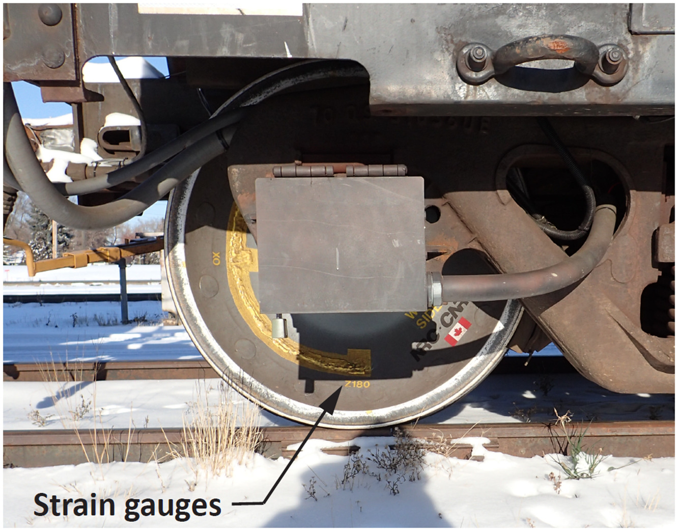
The IWS data collection was conducted as part of a larger investigation on track performance that included the instrumentation of a 15.8 m (52 ft) gondola car (Roghani et al. 2015, 2016, 2017a, b; Fallah Nafari et al. 2018a, b). The car was loaded with gravel to a total weight of 1,175 kN (264 kips). One end of the instrumented car was fitted with two IWS, each of which consist of one axle with two-wheel plates (Fig. 1). Each IWS wheel plate is 915 mm () diameter Class F and instrumented with 16 full-bridge Wheatstone strain gauge circuits, which are interpreted to forces applied to the wheels from the rail and resolve these forces into vertical, lateral, and traction forces for each of the four wheels (only vertical forces, i.e., dynamic loads are presented within this paper) (Woelfle 2016). The IWS was measured at a 200 Hz frequency and filtered with a 20 Hz low-pass filter was applied to the data during acquisition (Higgins et al. 1992; Bracciali 2014; Cakdi 2015; Barbosa 2016; Ren and Chen 2019). The latitude, longitude, time, and speed for each measurement was determined with a Garmin GPS18X global positioning system (GPS).
Each wheel of the IWS was calibrated individually in the laboratory before installation. Accuracy of the load measurements from the IWS are not provided with the instruments; however, the end of the car with the IWS had a static load of 576.2 kN measured by a scale after the installation of the IWS system, and this compares very favorably with the sum of the static loads from the four IWS wheels at 574.6 kN, a difference of 0.3%. The wheels had very little wear and were free of defects that would increase dynamic loads.
The section of track included in this study is operated by a Class 1 railway and is part of a high traffic subdivision [] through the Canadian Prairies. The studied section of track includes 30 bridges and overpasses, 50 switches, more than 100 grade crossings and approximately 83 km of curves. The rail is continuously welded and is supported primarily by concrete ties.
The IWS data used in this study was recorded over four passes of the study site, two in each direction, between July 2015 and August 2015, with maximum train speeds of . The passes were conducted with the car in revenue service (inserted within a freight train), thus without control over the type or weight of adjacent cars, or of the speed of travel. These limitations are common when conducting measurements on the track of a Class 1 North American freight railway. In total, the data base collected and evaluated within this study consisted of more than vertical dynamic load measurements.
Presentation of Results
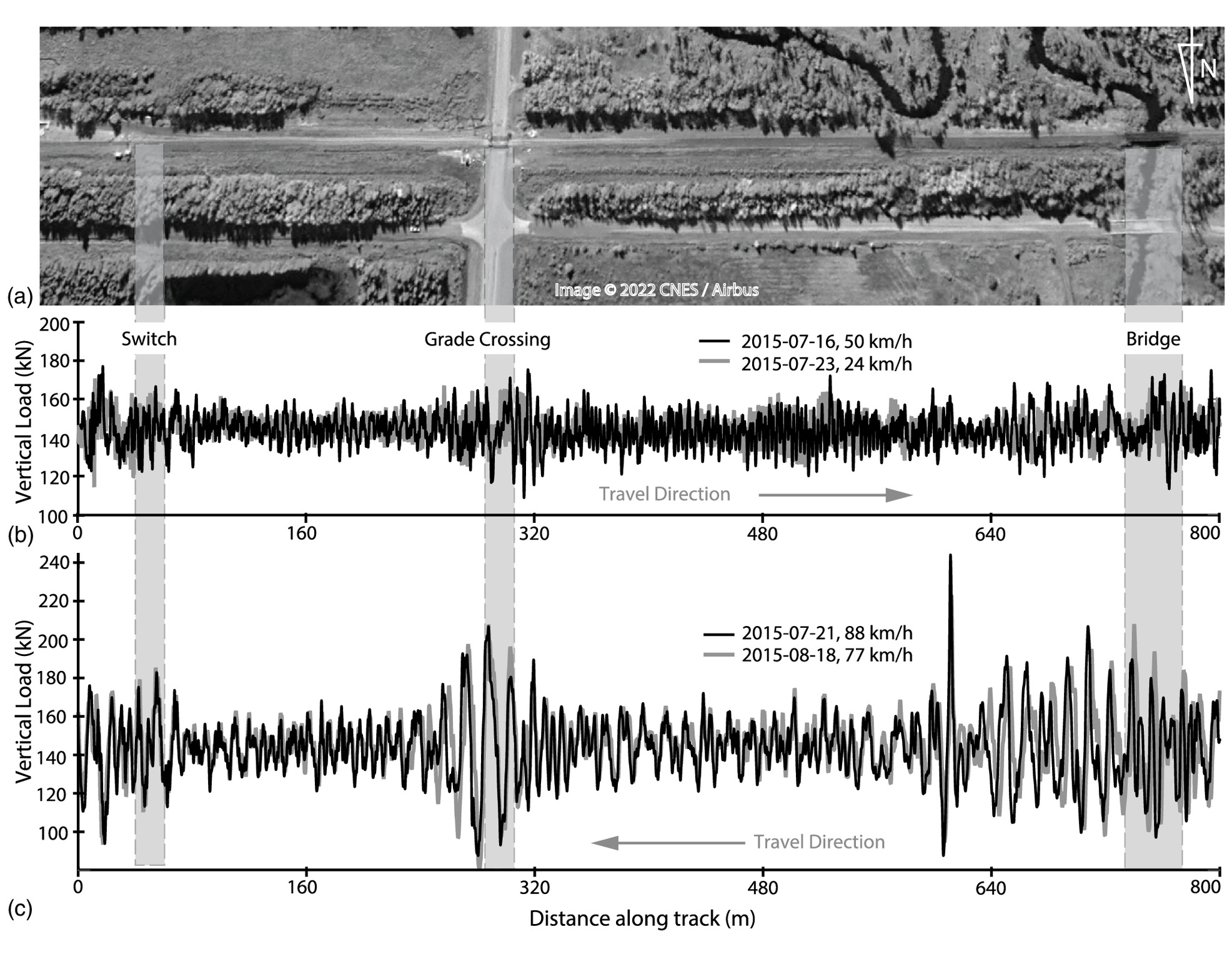
Examples of the resulting data are presented in Fig. 2 for an 800 m section of track that includes a switch, grade crossing, and a relatively short bridge [Fig. 2(a)]. This includes four passes of the instrumented car, two at slower speeds (24 and ) in the west-bound direction [Fig. 2(b)], and two at higher speeds (77 and ) in the eastbound direction [Fig. 2(c)]. The track features (switch, crossing, and bridge) initiate oscillations in dynamic loads that are clearly evident for the higher speed passes [Fig. 2(c)]. The magnitudes and pattern of dynamic loads are also remarkably similar and repeatable between the two higher speed passes in the same direction [Fig. 2(c)].
The distribution of the magnitude of measured vertical dynamic loads by track type (tangent and curve) and features (switch, crossing, and bridge) are presented in Fig. 3. This distribution was developed from all four IWS wheels and all four passes. There is a large disparity in the amount of data collected on each type of track, where tangent track comprised 69.9% of the measured data, curves comprised 24.7%, bridges comprised 1.6%, grade crossings comprised 2.2%, and switches comprised 1.6%. The statistical values that represent this distribution are presented in Table 3. These distributions are normal in nature and have mean and median values that are very close to the static load (144 kN) (Table 3). Tangent track has the narrowest distribution and thus the least number of extreme values [Fig. 3(a)]; this is followed by the curved track and bridges with very similar distributions [Fig. 3(b)], and grade crossings and switches, also with very similar distributions. The largest measured dynamic loads are measured on tangent track; however, the authors attribute this disproportionately greater data collection on tangent track. The highest 99.9th percentile dynamic vertical load occurs for switches, which is attributed the presence of the switch point.

| Track type | (kN) | Median (kN) | (kN) | Maximum (kN) | 99.9th (kN) |
|---|---|---|---|---|---|
| All | 143.9 | 144.1 | 11.3 | 384.4 | 177.9 |
| Tangent track | 143.9 | 144.2 | 10.9 | 384.4 | 176.5 |
| Curved section | 143.7 | 143.6 | 12.2 | 292.8 | 180.2 |
| Bridge | 144.6 | 144.6 | 12.4 | 288.9 | 181.9 |
| Grade crossing | 144.2 | 144.1 | 13.1 | 264.2 | 183.4 |
| Switch | 144.1 | 144.1 | 14.4 | 302.5 | 187.2 |
Note: Data includes all four instrumented wheels, and all four passes; = mean; = standard deviation; and 99.9th = 99.9th percentile.
Discussion
The equations are generated using the upper envelope of measured dynamic loads, such that they can be used as design loads. Using the maximum measured dynamic loads from the IWS system results in very high values (), significantly higher than predicted by any of the other equations () (Table 1) within the range of train speeds for which measurements at which IWS measurements were obtained. These are outlier values that need to be excluded and there are many methods to do so (ASTM 2021). Some of the existing equations were generated from using , or the 99.9th percentile, as an upper value exclusive of outliers (Sadeghi and Barati 2010), and this threshold is used within this analysis due to this precedence. An alternative method for the removal of outliers recommended by ASTM (2021) is the Grubbs’ test, which is effective for data sets with near normal distributions (Grubbs 1969; Pearson 2005) (Fig. 3). The Grubbs’ test determines a Grubbs’ value () at which is the mean value of the sample, is the standard deviation, is the value of the th element of the data set [Eq. (2)]
(2)
Fig. 4 presents the derived from the IWS measurements over tangent track, evaluated for increments for the maximum measured dynamic loads (inclusive of outliers), the 99.9th percentile value, and from the Grubbs’ test. The values in Fig. 4 are compared to Eq. (3) from AREMA (2021) and evaluated with the diameter of the IWS wheel, and Eq. (4) from Van Dyk et al. (2017)
(3)
(4)
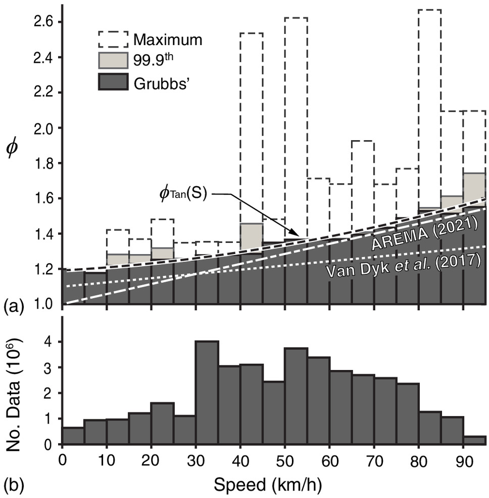
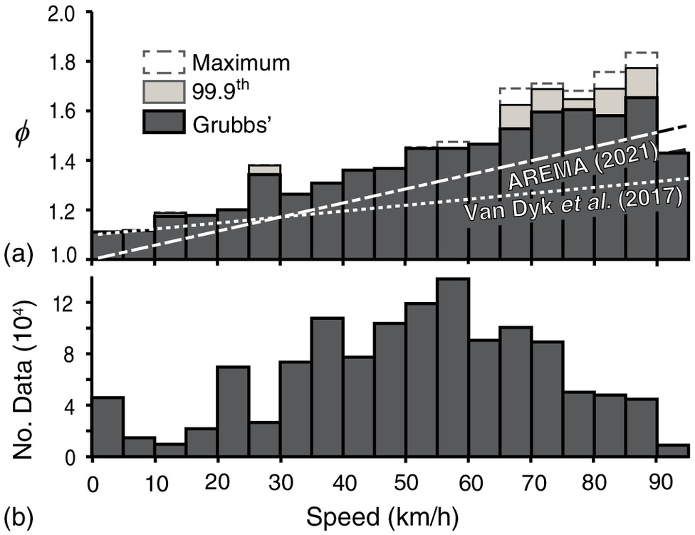
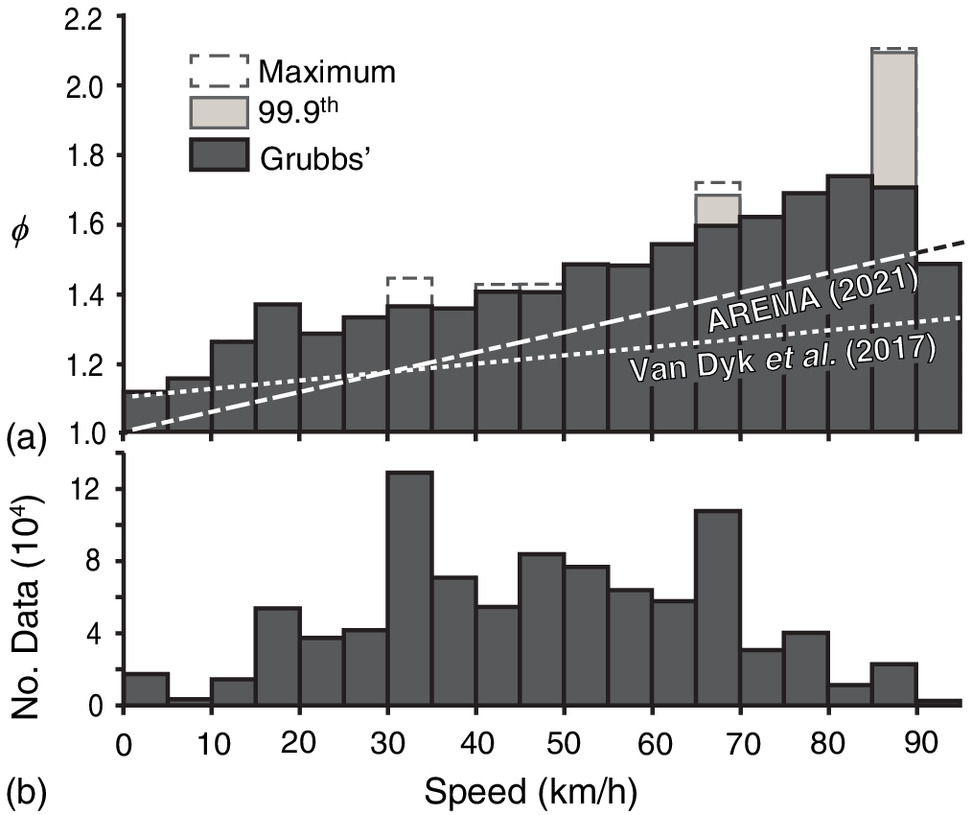
From Fig. 4 the evaluated from the Grubbs’ test for the removal of outliers consistently increases with increasing speed, whereas the evaluated from the 99.9th percentile is more variable. Also from Fig. 4, the AREMA (2021) equation [Eq. (3)] provides a close representation of the derived from the Grubbs’ test applied to IWS data from tangent track and train speeds in excess of . Eq. (3) increasingly underestimates with decreasing train speed below , approaching an underestimation of 0.2 below . The versus train speed plots similar to Fig. 4 were also generated for curved track (Fig. 5), bridges (Fig. 6), grade crossings (Fig. 7), and switches (Fig. 8), with poor representation by Eq. (3), which significantly underestimates the magnitude of dynamic loads on nontangent track. The data contained within each increment plotted in Figs. 4–9 is normally distributed with a mean and median value at (at static load). The trend in the is illustrated Figs. 4–9 as the 99th percentile magnitudes as this is . Qualitatively, Fig. 4 shows a strong consistent relationship between train speed and , suggesting a high reliability of threshold value, where each increment consisted of more than data points. The trends became less consistent, implying a lower reliability of threshold value, when the number of data point were below ; for example, Fig. 6 for speeds .
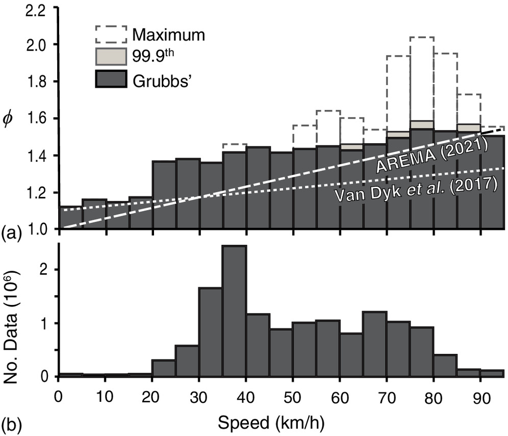
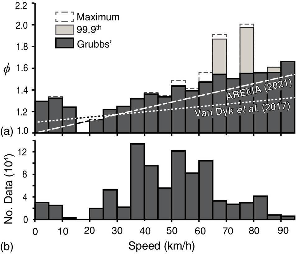
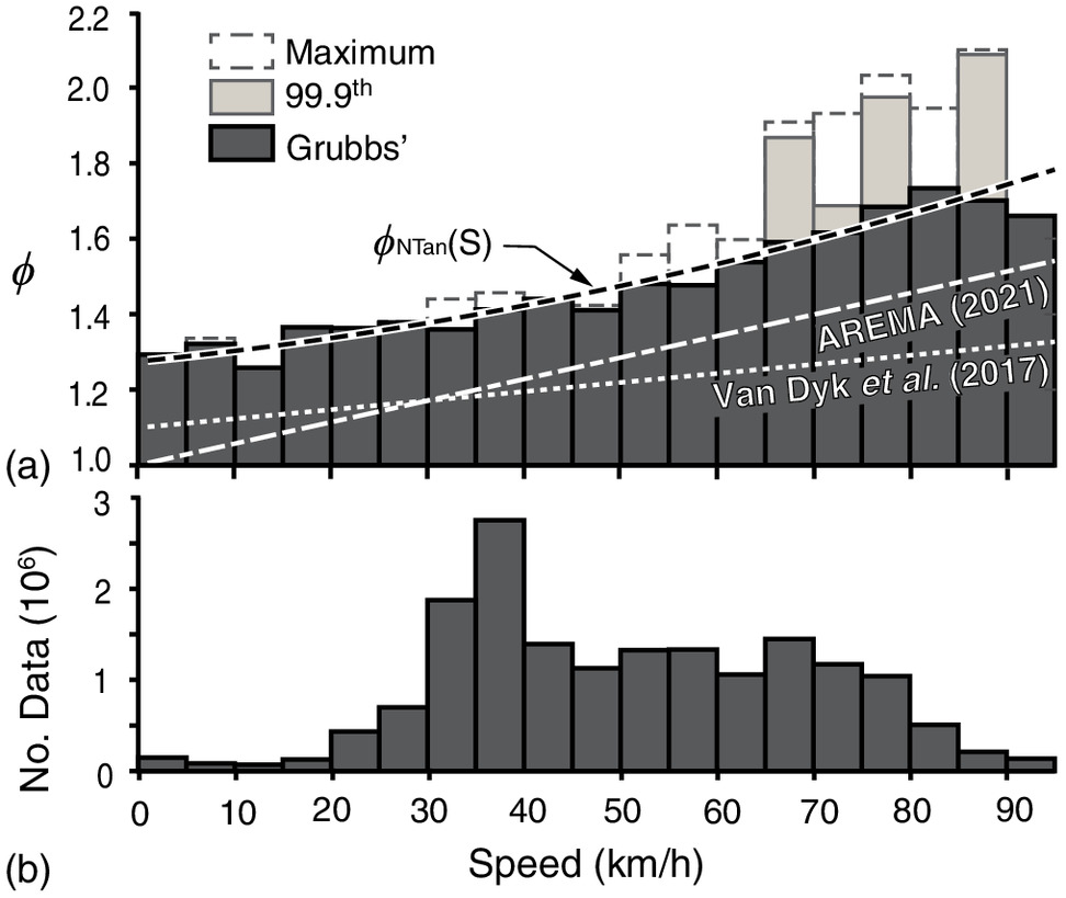
A quadratic equation fit to the values for tangent track derived using the Grubbs’ test, as a function of train speed, and is presented subsequently as Eq. (5). Thus, Eq. (5) defines the range of that tangent track may experience in service. Eq. (5) provides a close fit with an value of 0.97 also evident in Fig. 4. Equations developed for the other track types provided much poorer fits, the authors propose that the lesser amount of data at some speeds resulted in a greater variability. However, due to the similar statistical distributions of the measurements collected for grade crossings, switches, curves, and bridges in Fig. 3, all of these nontangent track data were grouped together and plotted in Fig. 9, and a quadratic equation fit to values derived using the Grubbs’ test was generated [Eq. (6)]. Eq. (6) provides a close fit with an value of 0.91 also evident in Fig. 9. Thus, Eq. (6) defines the range of that nontangent track may experience in service
(5)
(6)
As an alternative, and arguably more useful, presentation of the data was re-evaluated over the ranges of permissible train speeds within a given class of track (e.g., Class 2 track allows for train speeds from 0 to ) for each track type and presented within Table 4. The values in Table 4 then define the range of that class of track may experience in service.
| Class | Maximum speed [ (mph)] | AREMA [Eq. (12)] | Tangent | Curve | Bridge | Grade crossing | Switch | All nontangent |
|---|---|---|---|---|---|---|---|---|
| 1 | 16 (10) | 1.09 | 1.22 | 1.17 | 1.32 | 1.18 | 1.36 | 1.36 |
| 2 | 40 (25) | 1.23 | 1.28 | 1.41 | 1.32 | 1.34 | 1.36 | 1.41 |
| 3 | 64 (40) | 1.36 | 1.37 | 1.44 | 1.43 | 1.46 | 1.54 | 1.54 |
| 4 | 97 (60) | 1.55 | 1.55 | 1.54 | 1.66 | 1.65 | 1.73 | 1.73 |
The IWS data and the presentation of the data within Figs. 4–9 provide a measure of as a function of speed. As the IWS wheelsets are of very low wear and free of defects, the dynamic loads measured from the IWS are a result of speed, the variation of track conditions and the dynamic characteristics of the car. Thus, as evident in the magnitudes of maximum and Eqs. (5) and (6) that define the range of that track may be subjected to, that the effect of track conditions is clearly substantial and exceed previous estimates [as provided by AREMA (2021)].
These measurements differ significantly from the data obtained from the measurements of instrumented track [such as those presented in Van Dyk et al. (2017) from WILD sites] in that those results were representative of the loads caused by different locomotives and car types, and differing conditions of wheels on a consistent track section; whereas the results presented within this paper are primarily a result of different track conditions encountered by the IWS system. The authors propose that the two studies are complementary; that neither the data obtained from the measurements of instrumented track or within this study wholly represent the dynamic loads imparted on the rails; the combined effect is anticipated to further increase the range of ; and future studies should combine these two measurement types.
Conclusion
This study analysed dynamic loads, in terms of , derived from data collected from IWS. This differs from past studies that have relied on instrumented sections of track. The instrumented sections of track capturing the magnitudes of dynamic loads from all car types and conditions that pass over the site, but under constant track conditions. The IWS provided measurements of dynamics loads under constant car type and conditions, but on the variety of track conditions found over 340 km of in-service track. The results of this study demonstrated that the impact of track conditions is significant, resulting in ranges of dynamic loads and that track may experience well in excess of that provided by common means of estimating, especially for nontangent track (inclusive of curves, switches, crossings and bridges). Equations of as a function of speed [Eqs. (5) and (6)] were developed to quantify this range. However, the authors propose that further work is yet required to develop ranges of dynamic loads and that incorporate both track conditions and variations in car type and condition.
Appendix I. Summary of the Dynamic Load Factors () Equations Presented in the Literature for Passenger Railways
Examples of equations for the upper envelope of and dynamic loads for passenger railways are presented as follows:where = train speed (); = wheel diameter (mm); = track modulus; = track maintenance condition; = speed factor; = upper confidence limits regarding the probability of exceedance; = static load (kN); = total rail joint dip angle (radians); = track stiffness at joints (); = unsprung load on one wheel (kN); and = acceleration due to gravity ().
(7)
(8)
(9)
(10)
(11)
(12)
(13)
(14)
(15)
Appendix II. Developed Equations in Miles per Hour ()
From Eq. (5)
(16)
From Eq. (6)
(17)
Data Availability Statement
IWS and track geometry data used during the study were collected jointly by CaRRL, the National Research Council Canada (NRC), and the host railway. All position data recorded during this study are confidential in nature and may only be provided with approval of the host railway.
Acknowledgments
The authors would like to thank the Canadian National Railway for their support and facilitation of this project. Specifically, Tom Edwards for facilitating the collection of these data sets. This research was made possible through the Canadian Rail Research Laboratory (www.carrl.ca). Funding was provided by the Natural Sciences and Engineering Research Council of Canada (NSERC-IRC 523369-18), Canadian National Railway, the National Research Council of Canada, and Transport Canada.
References
AREMA (American Railway Engineering and Maintenance of Way Association). 2021. Manual for railway engineering. Lanham, MD: AREMA.
ASTM. 2021. Standard practice for dealing with outlying observations. West Conshohocken, PA: ASTM.
Barbosa, R. S. 2016. “Evaluation of railway track safety with a new method for track quality identification.” J. Transp. Eng. Part A Syst. 142 (11): 04016053. https://doi.org/10.1061/(ASCE)TE.1943-5436.0000855.
Birmann, F. 1965. “Paper 5: Track parameters, static and dynamic.” In Proc., Institution of Mechanical Engineers, 73–85. London: SAGE.
Bracciali, A., F. Cavaliere, and M. Macherelli. 2014. “Review of instrumented wheelset technology and applications.” In Proc., 2nd Int. Conf. on Railway Technology: Research, Development and Maintenance, 1–16. Stirlingshire, Scotland: Civil-Comp Press.
Cakdi, S., S. Cummings, and J. Punwani. 2015. “Heavy haul coal car wheel load environment: Rolling contact fatigue investigation.” In Proc., Joint Rail Conf., American Society of Mechanical Engineers Digital Collection. Washington, DC: ASME.
Doyle, N. F. 1980. Railway track design: A review of current practice. Canberra, WA: Australian Government Publishing Service.
Dybala, J., and S. Radkowski. 2013. “Reduction of Doppler effect for the needs of wayside condition monitoring system of railway vehicles.” Mech. Syst. Sig. Process. 38 (1): 125–136. https://doi.org/10.1016/j.ymssp.2012.03.003.
Esveld, C. 2001. Modern railway track. Zaltbommel, Netherlands: MRT-Productions.
Fallah Nafari, S., M. Gül, M. T. Hendry, and J. R. Cheng. 2018a. “Estimation of vertical bending stress in rails using train-mounted vertical track deflection measurement systems.” Proc. Inst. Mech. Eng., Part F: J. Rail Rapid Transit 232 (5): 1528–1538. https://doi.org/10.1177/0954409717738444.
Fallah Nafari, S., M. Gül, M. T. Hendry, D. Otter, and J. J. Roger Cheng. 2018b. “Operational vertical bending stresses in rail: Real-life case study.” J. Transp. Eng. Part A Syst. 144 (3): 05017012. https://doi.org/10.1061/JTEPBS.0000116.
FRA (Federal Railroad Administration). 2007. Track safety standard compliance manual. Washington, DC: USDOT.
Grubbs, F. E. 1969. “Procedures for detecting outlying observations in samples.” Technometrics 11 (1): 1–21. https://doi.org/10.1080/00401706.1969.10490657.
Hay, W. W. 1982. Railroad engineering. New York: Wiley.
Higgns, R. L., D. E. Otter, and R. W. Martin. 1992. “High accuracy load measuring wheelset.” In Proc., 10th Int. Wheelset Congress: Sharing the Latest Wheelset Technology in Order to Reduce Costs and Improve Railway Productivity, 181–187. Barton, ACT, Australia: Institution of Engineers.
Leishman, E. M., M. T. Hendry, and C. D. Martin. 2017. “Canadian main track derailment trends, 2001 to 2014.” Can. J. Civ. Eng. 44 (11): 927–934. https://doi.org/10.1139/cjce-2017-0076.
Pearson, R. K. 2005. Mining imperfect data: Dealing with contamination and incomplete records. Philadelphia, PA: Society for Industrial and Applied Mathematics.
Peters, N. 2010. CN railway engineering course. Montreal: McGill Univ.
Prause, R. H., H. C. Meacham, H. D. Harrison, T. G. John, and W. A. Glaeser. 1974. Assessment of design tools and criteria for urban rail track structures: Volume I. At-grade tie-ballast track. Washington, DC: DOT, Urban Mass Transportation Administration Office of Research and Development.
Ren, Y., and J. Chen. 2019. “A new method for wheel–rail contact force continuous measurement using instrumented wheelset.” Veh. Syst. Dyn. 57 (2): 269–285. https://doi.org/10.1080/00423114.2018.1460853.
Roghani, A., and M. T. Hendry. 2016. “Continuous vertical track deflection measurements to map subgrade condition along a railway line: Methodology and case studies.” J. Transp. Eng. Part A Syst. 142 (12): 04016059. https://doi.org/10.1061/(ASCE)TE.1943-5436.0000892.
Roghani, A., and M. T. Hendry. 2017a. “Quantifying the impact of subgrade stiffness on track quality and the development of geometry defects.” J. Transp. Eng. Part A Syst. 143 (7): 04017029. https://doi.org/10.1061/JTEPBS.0000043.
Roghani, A., R. Macciotta, and M. Hendry. 2015. “Combining track quality and performance measures to assess track maintenance requirements.” In Proc., ASME/IEEE Joint Rail Conf. Washington, DC: ASME.
Roghani, A., R. Macciotta, and M. T. Hendry. 2017b. “Quantifying the effectiveness of methods used to improve railway track performance over soft subgrades: Methodology and case study.” J. Transp. Eng. Part A Syst. 143 (9): 04017043. https://doi.org/10.1061/JTEPBS.0000071.
Sadeghi, J. 2012. “New advances in analysis and design of railway track system.” J. Reliability Saf. Railway 30 (3): 75–100.
Sadeghi, J., and P. Barati. 2010. “Evaluation of conventional methods in analysis and design of railway track system.” Int. J. Civ. Eng. 8 (1): 44–56.
Schramm, G. 1961. Permanent way technique and permanent way economy: With 23 tables. Ahmedabad, India: Elsner.
Srinivasan, M. 1969. Modern permanent way. Mumbai, India: Somaiya Publications.
TC (Transport Canada). 2011. Rules respecting track safety. Ottawa, ON, Canada: TC.
Van Dyk, B. J., J. R. Edwards, M. S. Dersch, J. C. J. Ruppert, and C. P. Barkan. 2017. “Evaluation of dynamic and impact wheel load factors and their application in design processes.” Proc. Inst. Mech. Eng., Part F: J. Rail Rapid Transit 231 (1): 33–43.
Woelfle, A. 2016. “Report for the national research council.” In Analysis of wheel-rail forces during (MRail) rolling deflection tests. Gloucester, ON, Canada: National Research Council Canada, Automotive and Surface Transportation.
Yu, F., and M. T. Hendry. 2019. “A new strain gauge configuration on the rail web to decouple the wheel–rail lateral contact force from wayside measurement.” Proc. Inst. Mech. Eng., Part F: J. Rail Rapid Transit 233 (9): 951–960. https://doi.org/10.1177/0954409718822870.
Information & Authors
Information
Published In

Journal of Transportation Engineering, Part A: Systems
Volume 148 • Issue 7 • July 2022
Copyright
This work is made available under the terms of the Creative Commons Attribution 4.0 International license, https://creativecommons.org/licenses/by/4.0/.
History
Received: Sep 25, 2021
Accepted: Feb 11, 2022
Published online: Apr 28, 2022
Published in print: Jul 1, 2022
Discussion open until: Sep 28, 2022
Authors
Metrics & Citations
Metrics
Citations
Download citation
If you have the appropriate software installed, you can download article citation data to the citation manager of your choice. Simply select your manager software from the list below and click Download.
Cited by
- S.I. Okocha, F. Yu, P.Y.B. Jar, M.T. Hendry, Use of a modified critical fracture strain model for fracture toughness estimation of high strength rail steels, Theoretical and Applied Fracture Mechanics, 10.1016/j.tafmec.2023.104069, 127, (104069), (2023).