Advancing Railway Asset Management Using Track Geometry Deterioration Modeling Visualization
Publication: Journal of Transportation Engineering, Part A: Systems
Volume 148, Issue 2
Abstract
Railway tracks need to be monitored to ensure safe operations and cost-effective maintenance. The monitoring is commonly conducted using a track recording car that describes deviations from an ideal track geometry. Over time, the measurements provide time series data that can be used to model the observed track geometry deterioration process. However, without simplification, the modeling results are generally too complex to be utilized to their full extent in track asset management. Therefore, this study aimed to implement visualization techniques for track geometry deterioration modeling results analysis which benefit track asset management. The best practices on track geometry deterioration modeling were studied and applied to the track geometry history of a track section located in Finland. After testing the establishing modeling principles, proposals were made regarding the use of the results in practice. This paper presents visualization techniques that use the modeling results of individual cross-sections to generate information about longer sections of track and even whole rail networks. These visualizations digest the massive amount of information from the modeling and present it in an informative way for practitioners to utilize and benefit from. Thus, this study fills the gap between research and practice in railway track geometry deterioration modeling.
Introduction
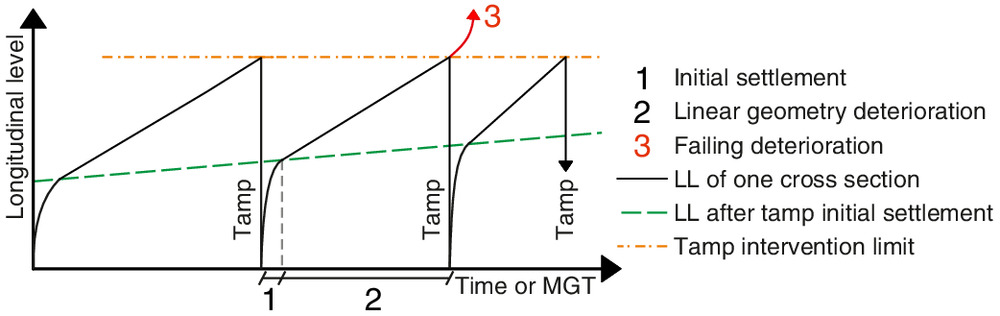
Multiple studies have demonstrated that track geometry deterioration is not a random process, but one that can be idealized and modelled [see Higgins and Liu (2018) and Soleimanmeigouni et al. (2018) for literature reviews]. Fig. 1 presents the idealized track geometry deterioration behavior of one cross section, which is always tamped at the exact same longitudinal level (LL) deviation value, and tamping always corrects the geometry to the original level. The figure demonstrates the theoretical diminishing effect of tamping due to fouling of ballast (Shenton 1985; Dahlberg 2001; Lichtberger 2011). In Phase 1 of Fig. 1, initial settlements increase deviations at an exponential pace. This is sometimes referred to as ballast memory. Following the initial settlement, Phase 2 describes a linear deterioration path that generally ends when a tamping intervention limit is reached. This is followed by a theoretical failing phase (3), which describes the track end-of-life, but in practice, this phase is avoided either by conducting maintenance or ceasing traffic.
Neuhold et al. (2020) provided a foundation for modeling track geometry deterioration based on actual track geometry car measurements. This approach was based on modeling the behavior of one cross section, thus providing results for a localized point on a track section, as longer sections of track were out of scope in that research. The current study extends the work of Neuhold et al. (2020) and demonstrates how track geometry deterioration modeling of cross sections can be utilized for investigating the behavior of not only cross sections, but also of longer sections of track and even the whole rail network.
Modeling track geometry deterioration based on track geometry car measurements provides highly practical information about the development of the condition of railway tracks. However, the real-world benefits of track geometry deterioration modeling can be obtained only if the modeling results are made accessible and understandable to practitioners in asset management. For this purpose, the results need to be generalized into key figures and representative visualizations that serve the heuristic nature of decision making in track asset management. Otherwise, the results achieved in academia will not have an impact in practice. The, this study also investigated indicators and visualizations created from track geometry deterioration modeling that would be beneficial to practical track asset management. The purpose was to ease the interpretation of the modeling results by providing summarized information for decision making, thus filling the gap between research and practice on track geometry deterioration modeling.
Two research questions were formed based on these research gaps:
1.
How to use cross-section-based track geometry deterioration modeling for longer sections of track and for the whole rail network?
2.
How to present track geometry deterioration modeling results in a way that practitioners can easily interpret and benefit from?
The scope of this paper is limited to visualizing stochastic long-term modeling of longitudinal deviations measured periodically using a track geometry measurement car. The purpose of this paper is to adapt the best current practices of track geometry deterioration modeling and bring them closer to practical application using visualization techniques, not to create completely new modeling techniques or to validate current models.
Track Geometry Deterioration Modeling
The best practices for preparing data for track geometry deterioration modeling were elaborated by Neuhold et al. (2020). This study follows these established practices as closely as possible, but some adjustments needed to be made to suit the data measured in Finland. The purpose was not to advance the methods presented by Neuhold et al. (2020), but rather to alter the methods for the available data. Table 1 summarizes the slight differences between the track geometry deterioration modeling described by Neuhold et al. (2020) and the methods used in this study. The following subsections further elaborate these differences.
| Modeling principles | Neuhold et al. (2020) | This study |
|---|---|---|
| Initial data | 16-year track geometry car history from 4,400 km in 5 m increments | 10-year track geometry car history from 60 km in 0.25 m increments |
| Geometry index | LL 100 m continuous modified SD | LL 200 m continuous SD |
| Alignment correction | None | None |
| Modeling method | Linear regression | Robust linear regression |
| Outlier handling | Outlier detection algorithm MAD | Robust linear regression |
| Tamping activity identification | Tamping records and negative TGDR | Negative TGDR and tamping area identification algorithm |
| Prognosis accuracy measure | Prediction and real end quality comparison | Prediction interval |
Initial Data
The data used for the demonstrations in this paper consists of a ten-year semi-annual track geometry car measurement history from a track section, Luumäki–Imatra, in Finland. The examined section is a 53 km long mixed traffic single line track section with a maximum speed of for passenger trains. The yearly gross tonnage of freight traffic is around 12 megatons. The measurements were preformed using an EM120 track recording car (Plasser & Theurer, Linz, Austria), which uses chord measurements from three bogies spaced 5 and 7 m apart. The data is recorded every 0.25 m. No major renewals were reported during this time period; only routine maintenance. Neuhold et al. (2020) used similar data, but their initial data was much more extensive, albeit measured more sparsely. Nevertheless, these differences do not matter, as the purpose of this study is to visualize the results, which does not require such a vast initial data set that statistical analyses require.
Track Geometry Parameter and Index
For long-term track geometry deterioration modeling, the LL standard deviation (SD) is commonly the chosen parameter, as most of the gradual displacements occur in the vertical direction (UIC 2008; Vale and Calçada 2014). SD provides a smooth depiction of the original deviation signal, and is defined as follows:where = the current value of a signal; = the mean value of a signal; and = the number of values in a sample (Eurocode EN13848-6 2014). Neuhold et al. (2020) opted for a modified SD, in which both the left and right rail were considered simultaneously, and the result was multiplied by 1.35 to make the result comparable with a conventional SD. This approach could not be adopted for this study, because reliable data repositories were available only for the left rail. This does not affect the end results of this study, as the applied visualization techniques are applicable to examining each rail individually or simultaneously.
(1)
SD can be calculated in fixed (also referred to as segmented) or rolling (also referred to as moving or continuous) windows, using any distance. Fixed SD calculation windows tend to be easier to communicate, but they misrepresent information when deviations occur in the edges of windows or if there are only local irregularities in the middle of otherwise stable track, as demonstrated by Neuhold et al. (2020). The use of rolling windows was found suitable for the data in Neuhold et al. (2020), as well as for this study.
Adjusting the length of the rolling window influences the sharpness with which the SD follows the original signal (Fig. 2). The appropriate rolling SD calculation window length can be considered to be roughly between 10 and 200 m, based on the lengths used in previous research (Andrade and Teixeira 2011; Tanaka et al. 2018; Neuhold et al. 2020; Audley and Andrews 2013). A shorter window SD more sharply follows the original signal, but too short a window might result in the same problems as those encountered when using only the original signal, namely, instability in alignment and a fluctuating signal. Too long a window may cause similar problems to those faced when using fixed windows, where some irregularities may be hidden due to adjacent smooth track.
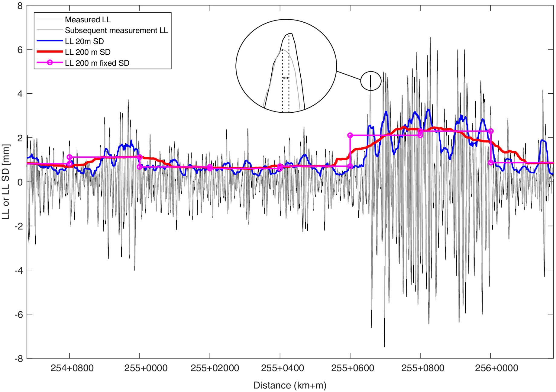
This study opted for a 200 m SD window, as there were some alignment issues between sequential measurements, as presented in Fig. 2. Neuhold et al. (2020) experienced similar problems and opted for a 100 m SD window. Furthermore, this study preferred the 200 m over the 100 m SD, because the 200 m SD is recognized by the European Standard 13848-6 (2014), which gives a good basis for standardizing the modeling principles and results.
Core Modeling Methods for Track Geometry Deterioration
Modeling the track geometry deterioration rate (TGDR) on a large scale requires a general depiction of past behavior, for example, when analyzing the decade-long behavior of a track section. Therefore, tamping intervals are usually adopted as the minimum interval length for a deterioration period. This leads to a simplification of the TGDR by using some mathematical idealization. The core mathematical approaches to LL SD deterioration modeling are linear and exponential modeling. Linear modeling of track geometry deterioration is the most popular modeling approach, based on the literature (Caetano and Teixeira 2015; Khajehei et al. 2019; Lee et al. 2018; Li et al. 2019; Neuhold et al. 2020; Nielsen et al. 2020; Soleimanmeigouni et al. 2020). In addition, it provides the best fit for the available data in Finland. However, it has been argued that exponential models suit some data sets better than linear models (Quiroga and Schnieder 2012; Famurewa et al. 2016). The use of exponential models can be justified by their ability to take the initial settlement into account. Generally, these models are suited better for track sections with high traffic volume and frequent (e.g., daily) track geometry measurements (Tanaka et al. 2018).
Real world measurements often provide outliers that need to be accounted for in modeling. Neuhold et al. (2020) used the mean absolute deviation (MAD) to identify and erase outliers. In this study, outliers could not be removed as in Finnish conditions they might indicate frost heave or other abrupt occurrences, which should be presented to asset managers. Therefore, outlier handling was considered when choosing the linear modeling method, not as a separate operation.
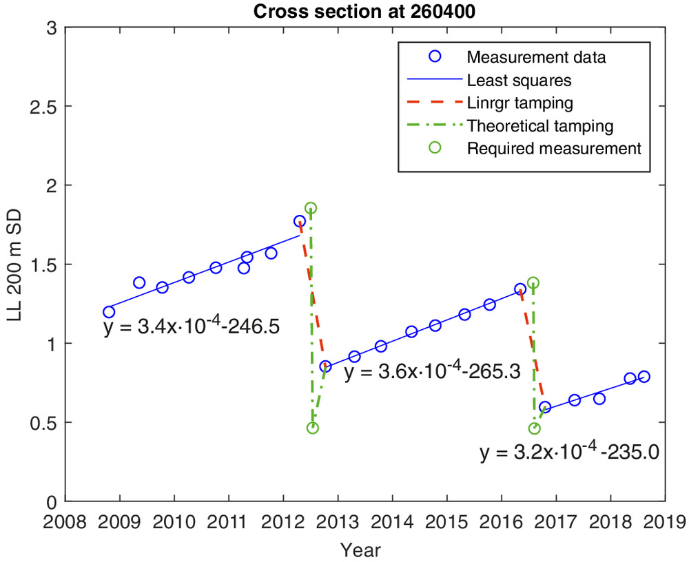
The linear regression modeling of geometry deterioration can be conducted using either simple or robust techniques. Simple techniques include algorithms such as least squares. These algorithms provide fast calculation times but tend to be influenced by outliers. However, outlier detection and removal algorithms can be run before using simple algorithms to improve the results. Robust algorithms, such as linear programming, generally produce numerous possible estimations and choose the best-fitting one. A plot of the differences between the algorithms (Fig. 3) depicts how in the second tamping interval (measurements between 2011 and 2017) the robust algorithm better describes the long-term behavior than least squares, when the initial settlement is not regarded.
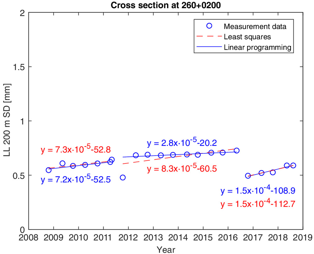
The major critique of all linear models is that they fail to capture the initial settlement behavior after tamping. The initial settlement lasts only days on a track section with heavy traffic, whereas the track geometry measurements are conducted every 2–6 months. Therefore, the probability of capturing the initial settlement caused by tamping in a track geometry measurement is low. This is not to say that it does not exist, but the recorded cases are few, and the effect of initial settlement on increasing deterioration is negligible when modeling on a large scale.
Fig. 3 presents a noticeable initial settlement captured by the track geometry measurements in 2011. However, the effects of the initial settlement on the linear regression can be eliminated by using a robust linear programming algorithm instead of simple techniques. Removing the effect of the initial settlement on linear regression modeling can be justified by arguing that capturing the long-term trend of the track geometry deterioration is more valuable than portraying the initial settlement. Furthermore, the initial settlement does not provide useful information about the deterioration, as the realized effect of tamping is the level of deviation after the initial settlement, as depicted in Fig. 1. Robust linear modeling ignores the initial settlement in the model, as is intended, but unlike outlier removal techniques, the outlier is left visible in the data, which is important, as these outliers can provide useful information to asset managers about the successfulness of tamping.
Tamping Identification
There are two main causes for a decreasing TGDR, namely, measurement inaccuracy and tamping (with or without other maintenance actions). The measurement inaccuracy usually accounts for only the slightest deterioration decreases, which are most likely to occur when the TGDR is close to zero. In these cases, the fluctuation in the measurement results is mostly attributed to the measurement technique rather than an improvement of the physical track geometry. These deterioration rates should be considered as zero in deterioration modeling. The decreasing deterioration due to tamping is usually clearly noticeable, especially in cases where the TGDR is not close to zero. However, modeling the tamping, i.e., the decreasing deterioration rate due to tamping, is very difficult due to multiple and generally unknown variables related to the timing and reason for tamping.
Solving the problem of what constitutes as tamping instead of measurement noise in the track geometry data is important, as tamping intervals form the basis for track geometry deterioration modeling. This problem can be overcome by systematically recording tamping data, but when the records are be incomplete or missing altogether, such as is the case in Finland, the solution must be applied in track geometry deterioration modeling.
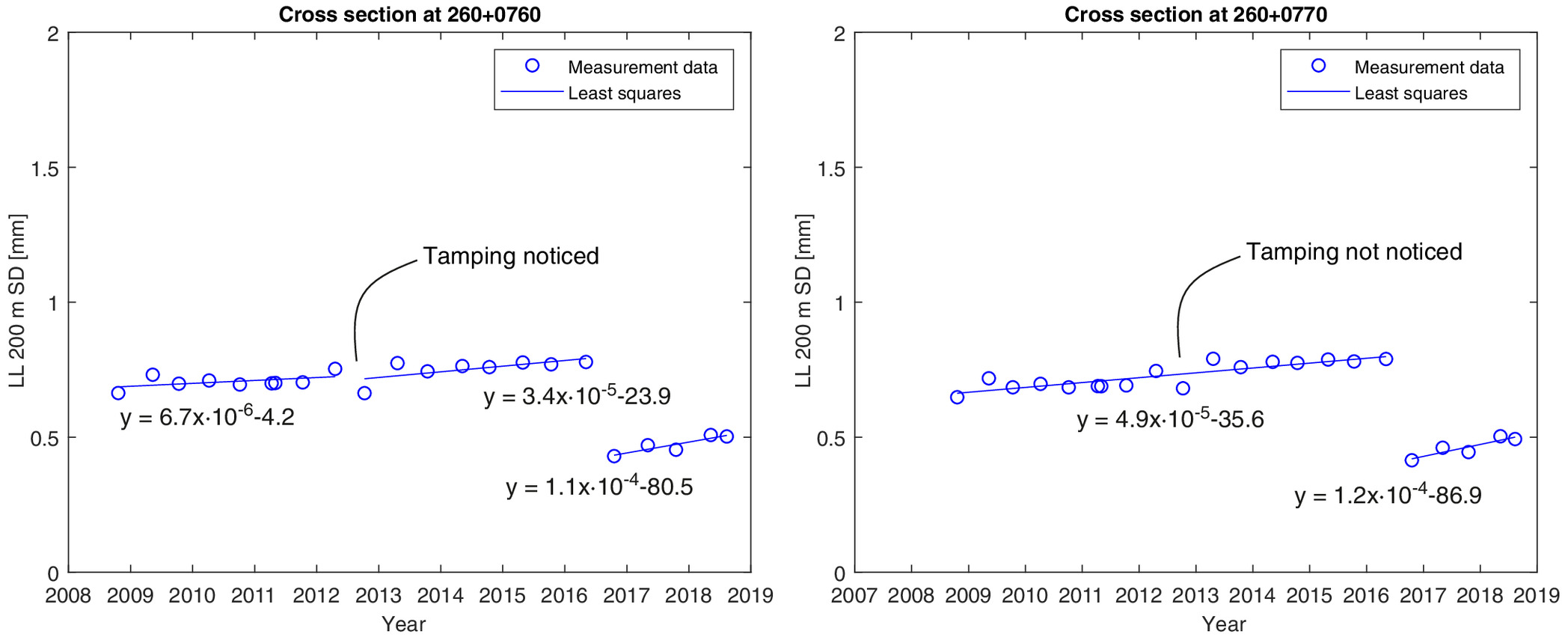
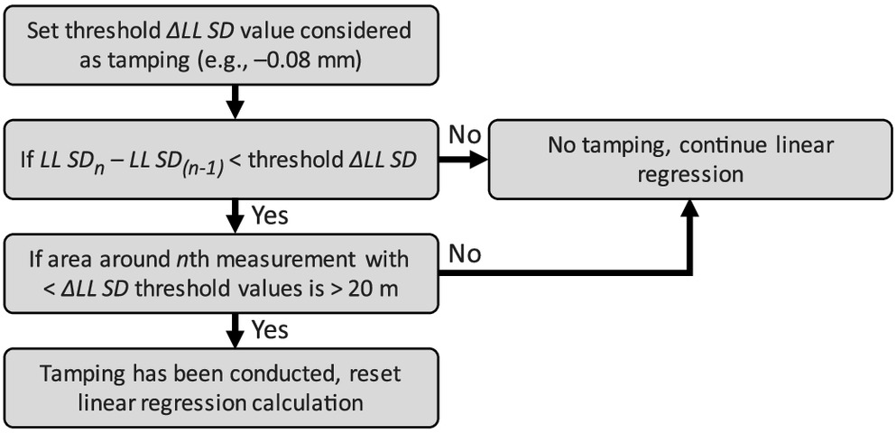
The simplest solution for revealing tamping in track geometry measurement data is to set a threshold for the decrease in the track geometry that will be considered tamping, as proposed by Neuhold et al. (2020). The threshold can be a fixed value or be dependent on time or deterioration level. A threshold value is adequate for detecting tamping that has had a significant effect on the irregularity level, which is suitable especially for segmented track geometry indices. However, when the LL SD is low before the tamping or the tamping has little effect on the LL SD, a threshold value will not consider these cases as tamping. This modeling case is common when modeling track geometry using a rolling SD. This issue is best demonstrated when the effect of tamping has roughly the same value as the limit for detecting tamping (Fig. 4). In these cases, on some of the cross sections in the tamped area a tamping is noticed, but on others, it is not. This leads to undesirable results, which are apparent when the sum of tamping times per cross section and the cross section LL SD histories are plotted (Fig. 4). These results will not be altered even with the use of a threshold dependent on the time or the irregularity level. All fixed thresholds for determining tamping will fail to separate tamping from measurement fluctuation in the cases of low irregularity levels, as the tamping effect on the irregularity is about the same amount as the measurement fluctuation. For that reason, an algorithm is required to determine these cases.
The algorithm created in this study searches the data for small individual areas with corrections in track geometry and disregards them as tamping if they are not associated with an adjacent tamped area. The generic form of the code is displayed in Fig. 5. The algorithm does not consider areas to be tamped if the area is less than a minimum length, which was set at 20 m in this study. Shorter areas with negative TGDRs were considered to have been caused by measurement inaccuracy. The accuracy of the algorithm could not be numerically verified, as there are no systematic historical tamping records in Finland. Verifying and improving the tamping detection algorithm is a source of further research.
Tamping Effect Quantification
The decrease in the level of irregularity calculated from track geometry car measurements before and after tamping indicates whether the tamping has successfully provided a stable ballast layer for the trains to pass, or whether the initial settlement cancelled much of the smoothness provided in the tamping. For example, in Fig. 6, tamping has had a meaningful effect on the level of irregularities, but in Fig. 3, irregularity has returned to the original state after one measurement in the second tamping interval, albeit the irregularities have stayed at a low level throughout the history.
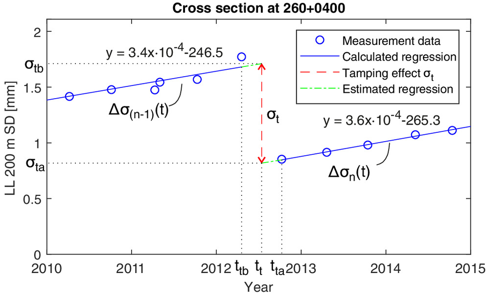
The effects of tamping, without considering the initial settlement after tamping, can be calculated using the information obtained from a robust linear regression model. A robust model is not prone to outliers, which means that if the initial settlement is captured in the first measurement after tamping, it will not be regarded in the results. Thus, the tamping effect describes the effect the tamping has had when regarding the long-term behavior.
The effect is calculated by extrapolating the regression lines before and after tamping to the time of tamping and calculating the difference in their irregularity level (Fig. 7). By doing so, the effect of tamping on the level of deterioration iswhere denotes the level of deterioration calculated from the line equation before tamping at the time of tamping ; and denotes the level of deterioration calculated from the line equation after tamping at the time of tamping . If the exact time of tamping is not known, it can be assumed that reasonable results can be obtained bywhere denotes the time of the first measurement after tamping; and denotes the time of the last measurement before tamping.
(2)
(3)
The TGDR after tamping is another important measure for determining the effectiveness of tamping. Tamping effectiveness can be determined by examining the deterioration rates before and after tamping. Higher deterioration rates after tamping indicate that problems continue after tamping, and thus, other maintenance actions together with tamping might be required in the future. Approximately equal deterioration rates before and after tamping indicate that tamping has reset the deterioration trend to a lower level, but the deterioration continues to develop as before. Deterioration rates that are lower after tamping than before tamping indicate that the tamping has had a remedial effect on the track structure.
The change in the TGDR () can be assessed by comparing the slopes of the linear track geometry deterioration models before and after tamping. There are three approaches to comparing the deterioration rates:
Absolute comparison
(4)
Relative comparison
(5)
Normalized absolute comparisonwhere denotes the deterioration rate of tamping interval ; and denotes the deterioration in the previous tamping interval. Because deterioration rates before and after tamping can be close to zero, relative or normalized absolute comparisons can result in very large or small values, due to the divisor or the dividend being close to zero, respectively. As an alternative, the absolute comparison does not suffer from this mathematical nuisance. However, because the absolute comparison does not normalize the deterioration rate of the previous tamping interval, the results should always be presented with knowledge of the level of the deterioration rate. Otherwise, the tamping effect might seem optimistic, if the deterioration rate before tamping has been very high. If information about the level of deterioration is incorporated, the absolute comparison is the most practical comparison to use. Otherwise, relative or normalized absolute comparison yields more informative results.
(6)
Evaluating past tamping effectiveness requires examining several figures simultaneously: the values of LL SD and TGDR after tamping, and the change in LL SD and TGDR due to tamping. Because simultaneous examination of four figures is not practical, an ensemble parameter representing their possible combinations is required. The ensemble parameter, named maintenance success indicator (MSI), can be assigned to represent four different outcomes of a tamping (Fig. 8): (1) beneficial, (2) delaying, (3) not meaningful, or (4) negative.
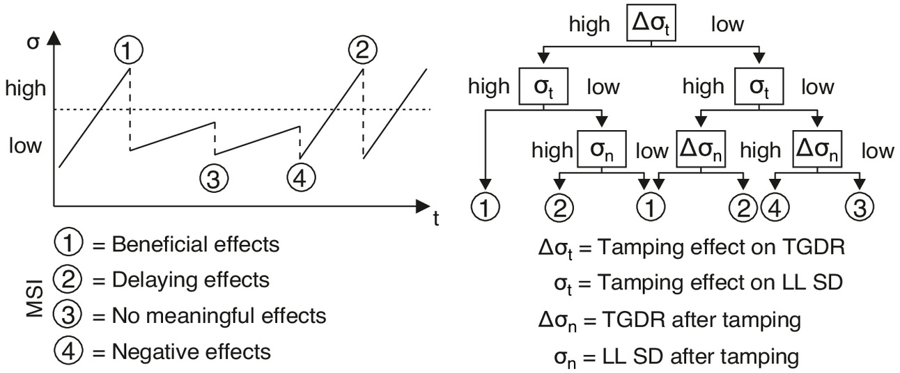
The logic behind MSI is presented in Fig. 8. The evaluation begins by assessing the effect of tamping on the TGDR (). If the effect on the TGDR () is high, it means that the deterioration rate has slowed down, and vice versa. Next, the tamping effect on the deterioration level () is evaluated. A high effect is the desirable outcome. Finally, the tamping interval after tamping is evaluated by assessing either the level of deterioration after tamping () or the TGDR after tamping (), where low values are the desirable outcome. The limit values separating high and low , , , and can be assessed using the allowable LL SD and limit values for TGDR. However, defining the limit values for these is out of scope and a source of future research, as the initial data for assessing the limit values should be much larger than the one available for this study.
A desirable outcome for the MSI is to have as much Class 1 (beneficial effects) tamping and as little of other classes. Areas with Class 3 or 4 effects should be closely investigated. The MSI Class 1 denotes that tamping has slowed down the TGDR and significantly reduced the LL SD, thus making the track behavior better than before tamping. MSI Class 1 can also be achieved, if the effect of tamping to TGDR or LL SD has been only slight if the TGDR and LL SD after tamping have been low. This implies that these values were low before tamping, therefore, they could not have been improved any further by tamping. Class 2 MSI implies that while the tamping has restored the LL SD, the TGDR is still high, meaning the tamping has been successful, but the remediation will not last. MSI Class 2 highlights areas where tamping is successful, but other maintenance actions are also required to obtain a lasting remediation. MSI Class 3 denotes that tamping has not made a significant difference, and perhaps the planned tamping areas should be revised, if possible. MSI Class 4 suggests that errors have been made in the tamping or that the track has suffered damage after tamping, and the area should be further investigated. Special cases, where a section is tamped before and after a measurement, must be considered separately as not applicable areas (n/a), as a TGDR cannot be calculated from a single track geometry measurement. The practical use of the MSI is presented in a later section, Visualizing Track Geometry Deterioration Modeling Results.
Prognosis and Prognosis Accuracy Measures
Predicting future LL SD values using linear regression models is simple. Extrapolating the linear regression model of the newest available tamping interval usually provides reasonably good results. However, if an area has been recently tamped, the insufficient number of measurements after tamping may not accommodate linear regression. In these cases, the linear regression model can be based on the previous tamping interval.
However, while the predictions of future LL SD values based on linear regression are simple to make, the predicted values themselves are not informative enough. The reliability of the predictions must be described as linear estimations have varying degrees of uncertainty. Neuhold et al. (2020) assessed prognosis accuracy by comparing the predicted and real end quality. However, this study could not adopt such a method, as the prognosis accuracy needs to be expressed for a future prediction.
The best way to describe the reliability of future predictions is by using the prediction interval (PI). The PI offers a simple way to describe where future observations (LL SD values) produced by the model will occur, with a specified confidence. The PI can be described in a generic form aswhere denotes the predicted timing of reaching a LL SD limit value; is the quantile of t-distribution having ; is the specified confidence level (for example 90%); is the square root of the residual sum of squares; is the covariance matrix of parameters; and is a column vector of the particular values of interest (LL SD limit value), at which the prediction is calculated (Agresti 2015).
(7)
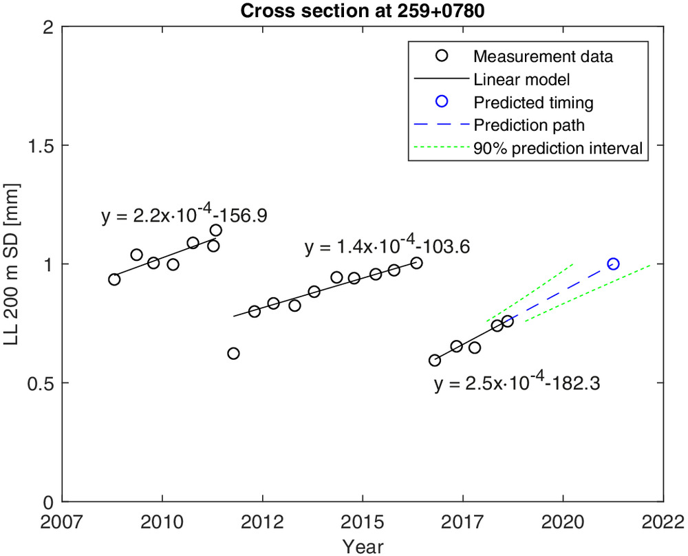
The PI does not provide a probability for a future observation but instead describes the level of confidence of the model predictions. For example, a 90% PI provides the range where approximately 90% of future observations produced by the model should occur. The PI can be communicated easily by plotting the range until a maintenance limit value is met. For example, in Fig. 9, the 90% PI indicates that the set maintenance limit of 1 mm LL SD is met between 2020 and 2022, and the most likely timing for reaching the limit is in 2021.
Visualizing Track Geometry Deterioration Modeling Results
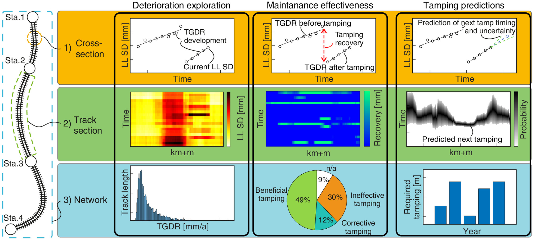
Asset management requires simple-to-use information that provides a good overall representation of the track conditions. The information from track geometry deterioration modeling should be reported for asset management in three categories: past deterioration exploration, past maintenance effectiveness evaluation, and future tamping need predictions. The scope of observation for each category should consider at least three levels:
1.
Cross section level
2.
Track section level,
3.
Network level.
The following sections elaborate what the different scopes and categories are used for and what novel information they produce.
Cross Section Level
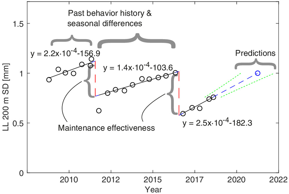
The cross section level scope provides the necessary tools for examining the track geometry deterioration of localized areas on a track section. The cross section here represents the 200 m LL SD values around that area. The analyses provide specific information about short problematic areas, for example, transition zones, which are more typical than long sections of poor condition track. The behavior of cross sections can be visualized in a time–LL SD perspective (Fig. 10). From these illustrations, the deterioration history can be observed, which includes the past changes in the TGDR and the past tamping times and their effects, and also, the timing of the next tamping can be predicted.
With these illustrations and results, the asset manager can answer, for instance, the following questions:
•
Is the cross section problematic (high TGDR)?
•
When had the problematic behavior begun?
•
Are there seasonal differences in the TGDR?
•
Has tamping been effective in maintaining good track geometry?
•
When will the area around the cross section require further maintenance?
By examining the past track deterioration behavior, maintenance effectiveness, and the predicted next maintenance intervention timing, the asset manager can guide maintenance by choosing the correct approach for remediation and time the remediation. In practice, the illustrations show whether the location has been tamped multiple times with no lasting improvement to the track geometry. In these cases, the asset manager can assign further investigations to determine appropriate spot repair to remedy the problem instead of tamping the area once again with futile effects. Furthermore, the asset manager can investigate the origins and development of problematic behavior, like seasonal differences or sudden increases in the deterioration rates caused by track work or extreme weather conditions. The asset manager also attains information on when the next maintenance action should be taken at that location.
Track Section Level
The track section-level scope of observation provides information on how the deterioration behavior differs within a longer section of track. The longer section of track is commonly between 1 and 10 km long, because even longer sections become difficult to assimilate. The goal is to detect problematic zones, so that the analysis can focus on those areas. The heatmaps of LL SDs [Figs. 11(a and c)], and tamping effects [Fig. 11(b and d)] can provide useful ways for analyzing the history of longer sections of track. The tamping effects here refer to the decrease in the LL 200 m SD.
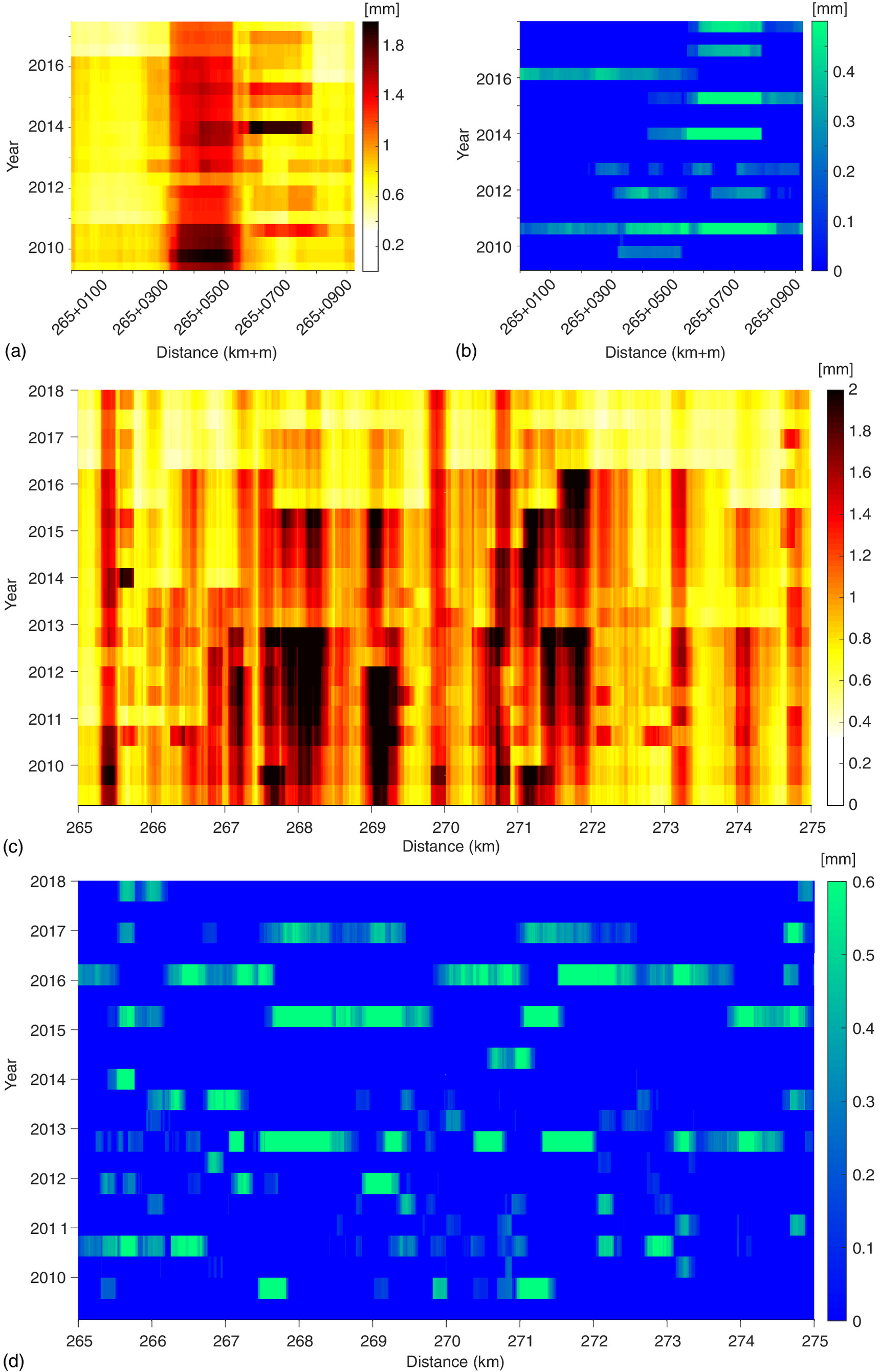
These figures should be examined together, as examining them separately does not provide sufficient information for reliable analysis. For example, in Fig. 11, the LL SD in the area around and remained at a rather high level until tamping in 2016, after which the LL SD has been moderately high, but tamping has not been required. This would lead to the conclusion that this area poses no concerns currently. Conversely, even though the LL SD in the area around and is moderate, the frequent tamping suggests that some problems do exist, but the tamping interval is so short that the track geometry measurements do not capture the actual behavior. This area should be closely monitored in future measurements.
In addition to assessing past deterioration behavior, predictions of the future tamping areas and their timing should be kept updated for asset management. The predicted tamping areas can be plotted with the principle presented in Fig. 12. The -axis indicates the location, whereas the -axis indicates the timing. The plot is color-coded to represent the PI of the predicted timing of the next tamping; a darker color indicates a more likely timing of the next tamping.
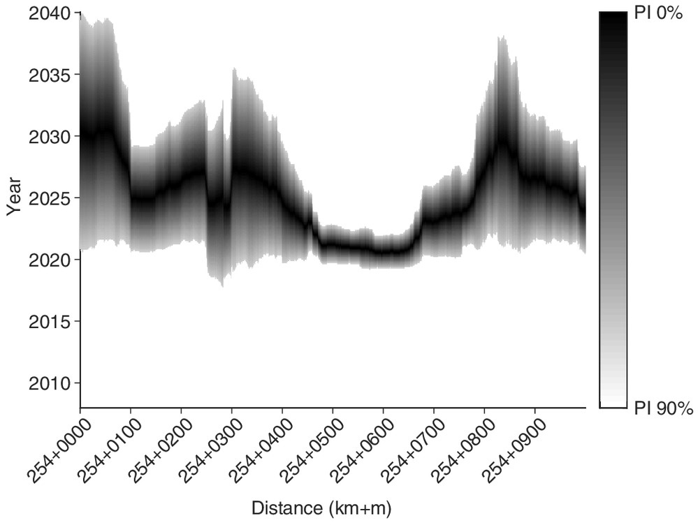
In track maintenance, the tamping timing prediction illustrations, like the one shown Fig. 12, can be utilized to plan future tamping areas. The graph also provides a general idea about the reliability of the predictions. For example, in Fig. 12, the LL SD in the area between and reaches a maintenance limit value at around 2022, and the PI is quite narrow. This would be a good indicator to plan tamping at that area for that year. As an example of another type of case, the area around and has a very wide PI, and it is predicted that tamping will be required around the year 2030. This area should not require tamping in the near future, but because the predictions are still ambiguous, the area should be focused on when new track geometry measurements are performed, and the predictions are updated.
With the information provided from the track section level analysis, the asset manager can answer the following questions:
•
Where are the problematic areas located on a track section, and how severe are they?
•
For how long has the problematic behavior been observed, and is it seasonal?
•
How has past maintenance affected the track geometry deterioration on the track section?
•
When will different parts of the track section require tamping or other maintenance?
The information obtained from illustrations following the principles shown in Figs. 11 and 12 can be used to guide maintenance by assessing the systemization of past maintenance, drafting tamping plans, and conducting the same analyses as for the cross section level, only now for a longer segment of track (e.g., 1–10 km). Past maintenance performance can be evaluated by visualizing the past tamping areas. Tamping areas disconnected from each other and frequently tamped areas indicate that tamping planning should be revised. Future tamping plans can be drafted using the illustrations by connecting areas with similar timing estimations for the next tamping. In addition, all the analyses mentioned for cross section level are valid for the track section level as well.
Network Level
Network-level track geometry deterioration assessment needs to represent complete track sections in generalizing figures and illustrations. The network-level analysis is intended to apply to tens or even hundreds of kilometers of track. For this purpose, the analysis turns to the statistics of the selected network. The past track geometry deterioration behavior of a network can be evaluated using a histogram displaying the number of track meters where a certain mean TGDR has been observed (Fig. 13).
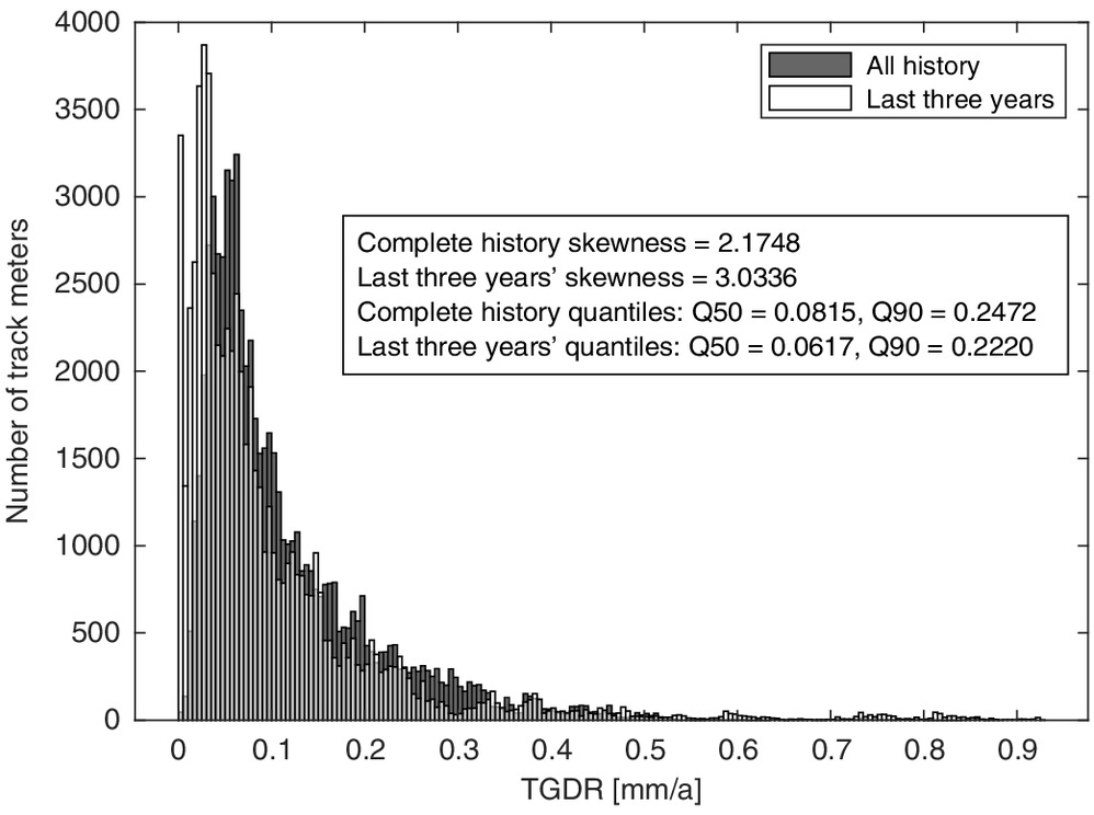
The histograms of the TGDRs observed on the track sections can be compared by plotting them in the same figure and then examining them. In addition to the visual examination of the histograms, key figures from the histograms can be produced to enhance the evaluation. The suggested approach is to report the median (50%) and 90% quantile of the distribution. The metrics on skewness should also be reported, as the histograms are often skewed to the right due to problematic areas exhibiting significantly larger deterioration rates compared to the median.
As an example of an analysis, Fig. 13 demonstrates two TGDR histograms from the same 60 km section of track: one containing the modeling of the complete 10 years’ measurements, and the other containing the modeling of the last three years’ measurements. At first glance, the last three years seem to be more to the left than the complete history, indicating that the conditions have improved on this section of track. This is supported by the lower median (50% quantile) and 90% quantile of the last three years compared with the complete history. However, the higher skewness on the history of the last three years suggests that the parts of the track enduring very poorly continue to be a problem.
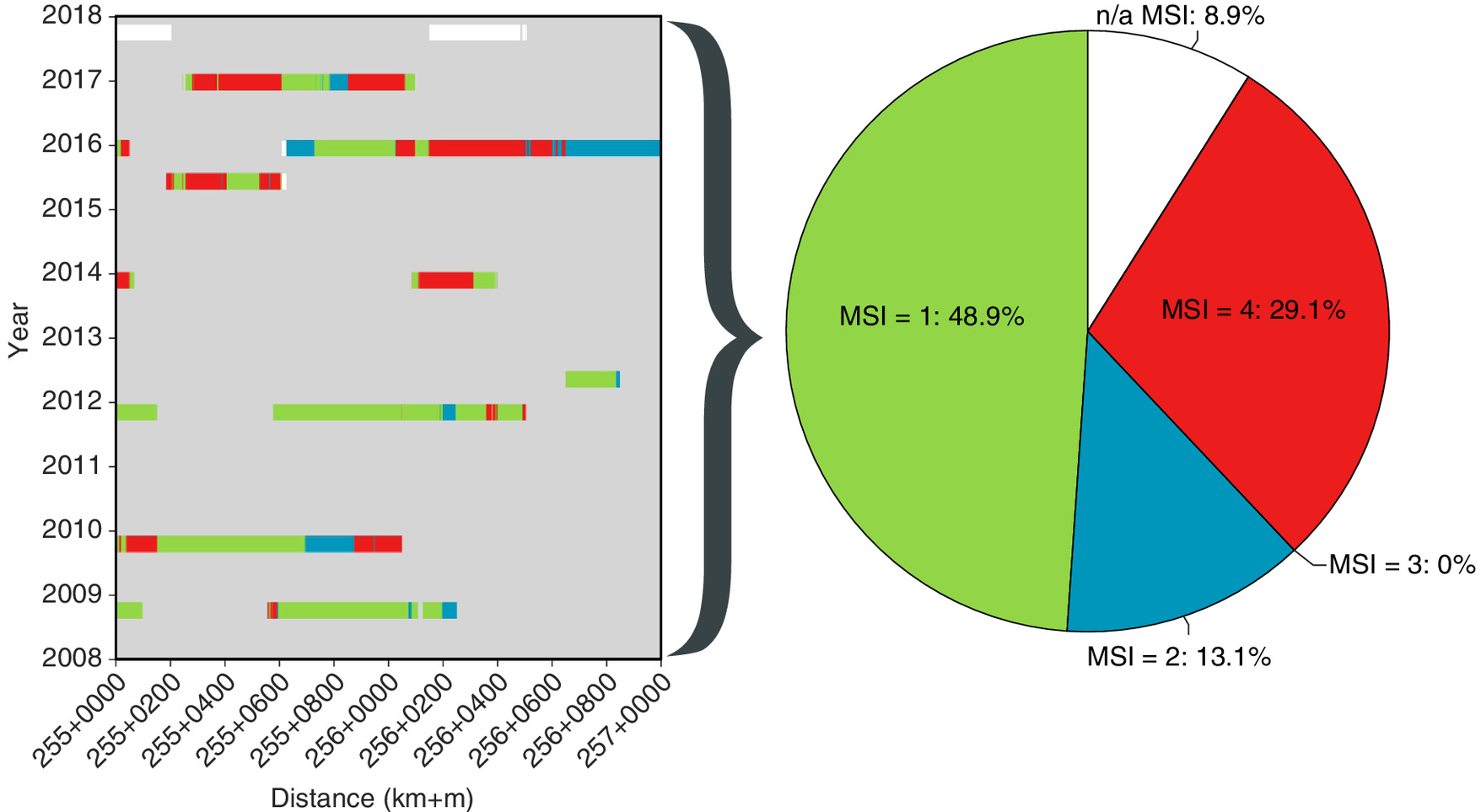
The network-level modeling result analysis should also review the past maintenance effectiveness by presenting the amount of effective tamping on the network. For this purpose, the MSI of tamping should be summarized by calculating the total amount and percentages of different MSIs on the network. Fig. 14 demonstrates how the tamping history of the MSI assessment is used for network-level analysis. The time–location view shows when and where tamping has occurred, and the color represents the MSI of the tamping. The pie chart shows a summary of the proportion of different MSIs on the observed section. If the MSI Categories 3 or 4 are overrepresented in the network summary pie chart, the asset manager can examine the areas where tamping has not been effective and further investigate those areas. This principle can be used for the network level, but for readability, the example contains only a two-kilometer long section of track. The information from the histograms and MSI summaries can be used to guide asset management in deciding when the next major renewal should be carried out, instead of performing routine maintenance. If the TGDR histogram shows a major part of the track section having a high TGDR, and MSI summaries imply that routine maintenance has had little effect on retaining sufficient track geometry, the asset manager should start preparing for track renewals.
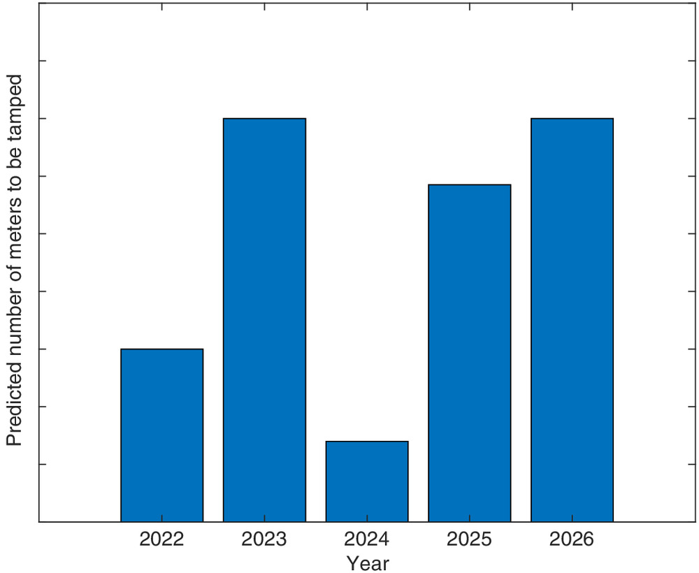
The network-level analysis also requires assessments of future tamping needs. These are best presented by a bar chart depicting the number of meters of track to be tamped in future years (Fig. 15). From illustrations like the one presented by Fig. 15, the asset manager can assess the need for maintenance funding and resources for the years to come. For example, if maintenance contracts are to be tendered, the asset manager can inform bidders about the expected amount of tamping required so that the amount of maintenance work and the number of tamping machines can be estimated. Furthermore, if the asset manager wants to represent the uncertainty in the estimations of future tamping needs, uncertainty can be calculated using, for example, a Monte Carlo simulation, as the linear models and PIs contain the necessary input data for simulating future observations; however the practical application for this is left for future research.
By combining the network level illustrations, the asset manager can answer the following questions:
•
What are the mean and extreme TGDR values on the network?
•
How has the TGDR evolved on a network level, and how do different networks compare?
•
Has tamping been effective on the network?
•
What is the expected amount of tamping on the network for the years to come?
Conclusion
This paper presented visualization techniques that help bring track geometry deterioration modeling from research into practice. In everyday asset management, the problem has been that track geometry deterioration modeling results are generally too complex and difficult to handle in daily operations. Therefore, this paper provided suitable visualization techniques, with which track geometry deterioration modeling results can be utilized by practitioners in asset management. This paper also demonstrated how modeling based on cross section data can be used for examining the track geometry behavior of longer sections of track and even for the whole rail network.
This study adapted the principles of track geometry deterioration modeling from the work of Neuhold et al. (2020), by slightly altering some aspects to better suit the data measured in Finland. The modeling approach was a robust linear model of a rolling 200 m LL SD. Future observation prediction accuracy was estimated using the PI, and past maintenance success was measured using the MSI. The proposed modeling methods are best suited for the LL SD, as it is generally observed to exhibit linear deterioration behavior. Other indices could work just as well, providing they follow linear deterioration behavior.
The main innovation of this study, i.e., how to connect suitable track geometry deterioration visualization techniques to different practical situations in asset management, is summarized in Fig. 16. The visualizations provide the following benefits:
•
The cross-section level analysis helps to analyze isolated defects, their history and future development.
•
The track section-level analysis provides a way to analyze longer sections of track to identify problematic areas and explore maintenance history, along with future maintenance timing.
•
The network level analysis summarizes the condition, past maintenance effectiveness, and future maintenance needs of complete track sections or even rail networks, into simple illustrations that help to make strategic decisions and allocate resources.
Lastly, several needs for future research were identified:
•
A reliable method for detecting tamping areas in the track geometry history without the use of tamping records should be established to enhance the accuracy of linear regression modeling.
•
The initial settlements after tamping should be further investigated to determine their duration in different circumstances and effect on relative and absolute track geometry.
•
Region-specific research on TGDRs and suitable limit values for them should be conducted to provide comparable TGDRs from different environments.
•
Uncertainty measures for the estimated amount of required future tamping should be defined.
Data Availability Statement
Some or all data, models, or code generated or used during the study are proprietary or confidential in nature and may only be provided with restrictions.
Acknowledgments
The authors want to thank the Tampere University Foundation Sr and the Finnish Transport Infrastructure Agency (Väylävirasto) for their valued co-operation.
References
Agresti, A. 2015. Foundations of linear and generalized linear models. 1st ed., 95–99. New York: Wiley.
Andrade, A. R., and P. F. Teixeira. 2011. “Uncertainty in rail-track geometry degradation: Lisbon-Oporto line case study.” J. Transp. Eng. 137 (3): 193–200. https://doi.org/10.1061/(ASCE)TE.1943-5436.0000206.
Audley, M., and J. D. Andrews. 2013. “The effects of tamping on railway track geometry degradation.” Proc. Inst. Mech. Eng., Part F: J. Rail Rapid Transit 227 (4): 376–391. https://doi.org/10.1177/0954409713480439.
Caetano, L. F., and P. F. Teixeira. 2015. “Optimisation model to schedule railway track renewal operations: A life-cycle cost approach.” Struct. Infrastruct. Eng. 11 (11): 1524–1536. https://doi.org/10.1080/15732479.2014.982133.
CEN (European Committee for Standardization). 2014. Railway applications. Track. Track geometry quality. Part 6: Characterisation of track geometry quality. Eurocode. Brussels, Belgium: CEN.
Dahlberg, T. 2001. “Some railroad settlement models—A critical review.” Proc. Inst. Mech. Eng., Part F: J. Rail Rapid Transit 215 (4): 289–300. https://doi.org/10.1243/0954409011531585.
Famurewa, S. M., U. Juntti, A. Nissen, and U. Kumar. 2016. “Augmented utilisation of possession time: Analysis for track geometry maintenance.” Proc. Inst. Mech. Eng., Part F: J. Rail Rapid Transit 230 (4): 1118–1130. https://doi.org/10.1177/0954409715583890.
Higgins, C., and X. Liu. 2018. “Modeling of track geometry degradation and decisions on safety and maintenance: A literature review and possible future research directions.” Proc. Inst. Mech. Eng., Part F: J. Rail Rapid Transit 232 (5): 1385–1397. https://doi.org/10.1177/0954409717721870.
Khajehei, H., A. Ahmadi, I. Soleimanmeigouni, and A. Nissen. 2019. “Allocation of effective maintenance limit for railway track geometry.” Struct. Infrastruct. Eng. 15 (12): 1597–1612. https://doi.org/10.1080/15732479.2019.1629464.
Lee, J. S., I. Y. Choi, I. K. Kim, and S. H. Hwang. 2018. “Tamping and renewal optimization of ballasted track using track measurement data and genetic algorithm.” J. Transp. Eng. Part A Syst. 144 (3): 04017081. https://doi.org/10.1061/JTEPBS.0000120.
Li, S., R. Liu, C. Li, and F. Wang. 2019. “Recovery measure of tamping on different track geometry irregularity indexes.” J. Transp. Eng. Part A Syst. 145 (11): 05019005. https://doi.org/10.1061/JTEPBS.0000274.
Lichtberger, B. 2011. Track compendium. 2nd ed., 393–396. Hamburg, Germany: DVV Media Group GmbH I Eurailpress.
Neuhold, J., I. Vidovic, and S. Marschnig. 2020. “Preparing track geometry data for automated maintenance planning.” J. Transp. Eng. Part A Syst. 146 (5): 04020032. https://doi.org/10.1061/JTEPBS.0000349.
Nielsen, J. C., E. G. Berggren, A. Hammar, F. Jansson, and R. Bolmsvik. 2020. “Degradation of railway track geometry—Correlation between track stiffness gradient and differential settlement.” Proc. Inst. Mech. Eng., Part F: J. Rail Rapid Transit 234 (1): 108–119. https://doi.org/10.1177/0954409718819581.
Quiroga, L. M., and E. Schnieder. 2012. “Monte Carlo simulation of railway track geometry deterioration and restoration.” Proc. Inst. Mech. Eng., Part O: J. Risk Reliab. 226 (3): 274–282. https://doi.org/10.1177/1748006X11418422.
Shenton, M. J. 1985. “Ballast deformation and track deterioration.” In Track technology, 253–265. London: Thomas Telford. https://doi.org/10.1680/tt.02289.0026.
Soleimanmeigouni, I., A. Ahmadi, and U. Kumar. 2018. “Track geometry degradation and maintenance modeling: A review.” Proc. Inst. Mech. Eng., Part F: J. Rail Rapid Transit 232 (1): 73–102. https://doi.org/10.1177/0954409716657849.
Soleimanmeigouni, I., A. Ahmadi, A. Nissen, and X. Xiao. 2020. “Prediction of railway track geometry defects: A case study.” Struct. Infrastruct. Eng. 16 (7): 987–1001. https://doi.org/10.1080/15732479.2019.1679193.
Tanaka, H., S. Yamamoto, T. Oshima, and M. Miwa. 2018. “Methods for detecting and predicting localized rapid deterioration of track irregularity based on data measured with high frequency.” Q. Rep. RTRI 59 (3): 169–175. https://doi.org/10.2219/rtriqr.59.3_169.
UIC (Union of Railways). 2008. Best practice guide for optimum track geometry durability. Railway technical publications. Paris, France: UIC.
Vale, C., and R. Calçada. 2014. “A dynamic vehicle-track interaction model for predicting the track degradation process.” J. Infrastruct. Syst. 20 (3): 04014016. https://doi.org/10.1061/(ASCE)IS.1943-555X.0000190.
Information & Authors
Information
Published In

Journal of Transportation Engineering, Part A: Systems
Volume 148 • Issue 2 • February 2022
Copyright
This work is made available under the terms of the Creative Commons Attribution 4.0 International license, https://creativecommons.org/licenses/by/4.0/.
History
Received: Jun 28, 2021
Accepted: Sep 30, 2021
Published online: Nov 24, 2021
Published in print: Feb 1, 2022
Discussion open until: Apr 24, 2022
Authors
Metrics & Citations
Metrics
Citations
Download citation
If you have the appropriate software installed, you can download article citation data to the citation manager of your choice. Simply select your manager software from the list below and click Download.
Cited by
- Stefan Marschnig, Peter Veit, Assessing Average Maintenance Frequencies and Service Lives of Railway Tracks: The Standard Element Approach, New Research on Railway Engineering and Transportation, 10.5772/intechopen.110488, (2024).
- Stefan Offenbacher, Christian Koczwara, Matthias Landgraf, Stefan Marschnig, A Methodology Linking Tamping Processes and Railway Track Behaviour, Applied Sciences, 10.3390/app13042137, 13, 4, (2137), (2023).
- Mikko Sauni, Heikki Luomala, Pauli Kolisoja, Kalle Vaismaa, Framework for implementing track deterioration analytics into railway asset management, Built Environment Project and Asset Management, 10.1108/BEPAM-04-2022-0058, 12, 6, (871-886), (2022).