Abstract
The statistical models supporting the Highway Safety Manual quantify associations between aggregate traffic measures, such as average daily traffic volume or posted speed limit, and crash frequencies accumulated over several years. For some time though, it has been recognized that crash risk can vary as traffic conditions vary due to special events or within-day changes in traffic. Additionally, the Highway Safety Manual’s predictive tools are essentially statistical summaries of conditions present during the recent past, and transferring this knowledge to environments containing automated vehicles is likely to be problematic. This paper illustrates how both issues can be addressed by supplementing standard statistical modeling with models describing crash mechanisms. In particular, Brill’s random walk model of how traffic shockwaves generate rear-end crashes is combined with a traffic flow model based on a fundamental diagram in order to quantify the relation between traffic density and rear-end crash risk. Approximating Brill’s random walk with a finite Markov chain leads to a computationally tractable model, and the model’s predicted relationship is consistent with empirical findings. Transferring the model to a hypothetical environment with automated vehicles is then illustrated.
Introduction
The Highway Safety Manual (HSM) (AASHTO 2010) offers evidence-based tools for predicting the safety effects of design-related decisions. These tools are applicable to a variety of road types (segments and intersections on two-lane rural highways, multi-lane rural highways, and urban and suburban arterials), they allow for a wide range of roadway features (e.g., lane and shoulder widths, presence of curves, roadside features), and they support a range of crash types (e.g., angle, rear-end, or pedestrian-involved). The HSM uses statistical regression models, called safety performance functions (SPF), to predict expected crash frequencies for specific base conditions and empirically-derived crash modification factors (CMF) to predict the effects of deviations from the base conditions. Although the HSM is a major advance in practical knowledge regarding road safety, HSM also has, as currently implemented, certain limitations. First, the HSM quantifies associations between aggregated traffic measures, such as posted speed limits or annual average daily traffic volumes (AADT), and crash frequencies accumulated over several years. Since crash risk can vary as traffic conditions vary, the current HSM offers only limited guidance on responding to exceptional events or managing within-day variations in traffic. This issue has been recognized and is currently the focus of an NCHRP project (NCHRP 2019b). Second, the predictive tools in the HSM were derived largely from statistical summaries reflecting the population of drivers and vehicles on the roads during the recent past. This population is expected to change, perhaps substantially, when and if automated vehicles (AV) achieve a significant market share, and it is not yet clear how design and operational practices should change in response. This is also the subject of an NCHRP initiative (NCHRP 2019a) and brings us to a more general issue, assessing the external validity of safety-related findings. In their classic work, Campbell and Stanley (1966) defined external validity as “generalizability of empirical findings to new environments, settings, or populations…” but, in road safety, assessing external validity has usually been presented as a problem of determining the transferability of SPFs and CMFs (FHWA 2015, p 25). Once the connection between transferability and external validity is made, however, we can see that this issue goes beyond road safety. In policy analysis, Cartwright and Hardie (2012, p. 6) have argued that determining if a policy “will work here” from the knowledge that “it worked somewhere” requires “facts about the causal role the policy plays and facts about the support factors that must be in place for the policy to work.” In medicine, Parkkinen et al. (2018) have argued that determining the external validity of a claim that “A causes B” requires that “the mechanism responsible for B in the target population is sufficiently similar to that responsible for B in the study population” (Section 2.3). Taking this as our guide, it appears that transferring the safety knowledge gained in one set of conditions to other situations requires understanding the processes, i.e., mechanisms, generating the relevant crash phenomena. Although the nature of mechanisms is an ongoing topic of philosophical debate, one reasonable definition has been put forward by Illari and Williamson (2012, p. 120): “A mechanism for a phenomenon consists of entities and activities organized in such a way that they are responsible for the phenomenon.” A case can be made that a significant portion of scientific activity, especially in the life sciences, is devoted to discovering and elucidating mechanisms (e.g., Machamer et al. 2000), and mechanism-based arguments, applied to reconstructed crashes, have been used to estimate potential safety benefits arising from vehicle automation (e.g., Haus et al. 2019; Kusano and Gabler 2012; Rosen et al. 2010). In these studies, kinematic models for types of road crashes were combined with numerical inputs describing the actions of the involved parties and the capabilities of vehicle/road systems. Inputs were then changed to reflect new situations, and the kinematic models were used to simulate revised outcomes. The fractions of crashes that, according to the simulations, would have been prevented were then taken as measures of AV impacts. In highway design, mechanism-based descriptions of critical events have been used to derive design constraints (AASHTO 2017), but for safety prediction, the focus has been on regression models like those supporting the HSM and their relatives, such as advanced heterogeneity models (Mannering et al. 2016).
In what follows, we argue that mechanism-based models provide tools both for addressing short-term variations in crash risk and for transferring current safety knowledge to environments containing AVs. Our argument is by example, using rear-end crashes on freeways. The section “Regression-Based Modeling of Rear-End Crash Risk” outlines our regression-based work that found inverted U-shaped relationships between traffic density and rear-end crash risk on several segments of Interstate Highway 35W. The section “Mechanism-Based Model of Rear-End Crash Risk” describes a mechanism model, originally due to Brill (1972), that when coupled with a fundamental diagram of traffic flow reproduces such inverted U-shaped relationships. In this model, the crash probability for a platoon of vehicles is related to the first-passage time of a random walk, and a tractable procedure for computing this probability is presented. The section “Transferring Knowledge to an AV Environment” then describes how the model developed in the section “Mechanism-Based Model of Rear-End Crash Risk” can be used to characterize the crash risk for a platoon of vehicles equipped with adaptive cruise control (ACC) and automatic emergency braking (AEB). Finally, the section “Summary and Conclusion” presents our conclusions and suggestions for future work.
Regression-Based Modeling of Rear-End Crash Risk
This section briefly reviews the literature on associations between traffic flow measures and crash risk on freeways and then introduces our recent work where logistic regression was used to control for the effects of traffic conditions in a before/after study of freeway improvements.
Compared to single-vehicle road departures, rear-end crashes on busy urban freeways are less likely to produce serious or fatal injuries, but they do generate much of the nonrecurring delay familiar to urban commuters. The fact that crash risk can vary with traffic conditions has been recognized for at least 20 years (Liu and Popoff 1997), leading to efforts at identifying those situations where crashes are more likely. Pioneering work in this area was performed by Oh et al. (2001) and Lee et al. (2002), with a focus on using inductive loop-detector data to identify short-term crash precursors. Abdel-Aty et al. (2004) introduced a case-control approach, where crash reports were reviewed in order to identify crashes occurring on a section of Interstate-4, and archived data from loop detectors were used to characterize traffic conditions. These crash events provided the cases for a case-control analysis, while control events were selected from the same locations, and at times similar to those of the crash events, but when no crashes had occurred. Logistic regression was then used to identify traffic measures that discriminated the cases from the controls. A model using average lane occupancy and the coefficient of variation of traffic speed as predictors detected 69% of the crash events. Subsequently, variants of this approach have led to significant improvements in predictive power, and Roshandel et al. (2015) have reviewed this work.
Our interest in modeling traffic conditions versus freeway crash risk is connected to recent work on estimating the safety-related impacts of a major set of improvements to Interstate Highway 35W (I-35W) (Davis et al. 2017). These improvements sought to reduce congestion on that part of I-35W running through the Twin Cities of Minnesota, and they included the conversion of the shoulder on a section of northbound I-35W to a priced dynamic shoulder lane (PDSL). Following the completion of the project, however, this PDSL section experienced both a substantial increase in traffic congestion due to the removal of an upstream bottleneck and a roughly three-fold increase in the frequency of rear-end crashes. It was unclear if this change in crash frequency was a direct effect of the PDSL or an indirect effect due to the relocation of traffic congestion. To untangle these effects, we employed an interrupted time-series design, with logistic regression being used to control for changes in traffic conditions.
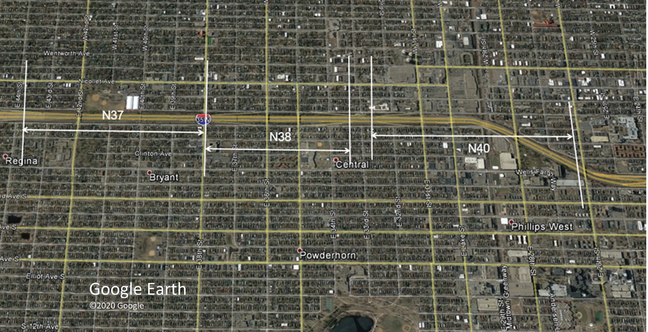
Fig. 1 shows a Google Earth image of northbound I-35W; the PDSL section was divided into three segments, each of which contained an inductive loop-detector station. Segment N37 was 1.34 km (0.83 mi) long, segment N38 was 0.84 km (0.52 mi) long, and segment N40 was 1.26 km (0.78 mi) long. Computerized records for crashes occurring in this area were identified for a before period running from January 1, 2004, to December 31, 2006, and an after period running from January 1, 2011, to December 31, 2013; hard copies of the original crash reports were reviewed to verify the type, location, direction, and time for each crash. Each hour in both the before and the after periods was then classified as to whether or not at least one rear-end crash had been reported during that hour. 30-second traffic counts and lane occupancy measurements were obtained for each segment’s loop-detector station for both the before and after periods. Lane occupancy was of particular interest because it is approximately proportional to traffic density (Garber and Hoel 2015). That iswhere = lane occupancy (percent), = traffic density (vehicles/km), and = effective vehicle length (meters).
(1)
The raw loop-detector data were screened for missing or obviously erroneous values, such as records showing negative volume or lane occupancy, records with occupancies greater than 100%, or records showing the repetitive patterns caused by failures to update the recording system’s buffers. Traffic flow, average lane occupancy, and the standard deviation of lane occupancy were then computed for each analysis segment and for each hour during both the before and after periods. In order to not confound traffic conditions leading to a crash with those caused by a crash, for each hour when a crash occurred, the traffic conditions were computed for the half-hour preceding the reported time of the crash. Eq. (2) shows the logistic regression model that was used to relate the probability of crash occurrence to traffic and weather measurements and to a dummy variable that captured the direct effect, if any, of the PDSLwhere , no crash occurred during hour ; , crash occurred during hour ; = row of the predictor variable matrix; and , = parameters to be estimated.
(2)
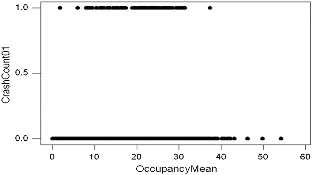
Initially, weather conditions (whether or not rainy or snowy conditions were present during that hour), traffic volume (vehicles/hour), average lane occupancy, lane occupancy standard deviation, and whether or not that hour occurred before or after the construction of the PDSL were all included as predictors of rear-end crash risk, and the maximum likelihood method was used to fit and evaluate different combinations of the predictors. This process has been described in detail (Davis et al. 2017), and here we simply summarize some especially relevant findings. We found that our initial models had difficulty passing routine goodness-of-fit tests, and Fig. 2 plots the occurrence or nonoccurrence of rear-end crashes versus lane occupancy for PDSL segment N38. Consistent with findings reported by Xu et al. (2014), crashes were most frequent when lane occupancy took on mid-range values and were less frequent when lane occupancy was either low or high. These considerations suggested that our models should allow for a possibly concave relationship between lane occupancy and crash risk, and a quadratic term for lane occupancy was added to the predictor list. Table 1 shows the final model selected for segment N38 and includes only those predictors whose coefficients were significantly different from zero. In particular, the coefficient for the variable indicating the presence/absence of the PDSL was insignificant, indicating no direct effect from the PDSL. Note though that both lane occupancy and lane were included and that the coefficient for lane was negative, indicating a concave region for the fitted risk curve.
| Variable | Estimate | Standard error | Z-statistic | P-value |
|---|---|---|---|---|
| Constant | 0.259 | 0 | ||
| Lane occupancy | 0.37403 | 0.0455 | 8.222 | 0 |
| Lane | 0.00177 | 0 |
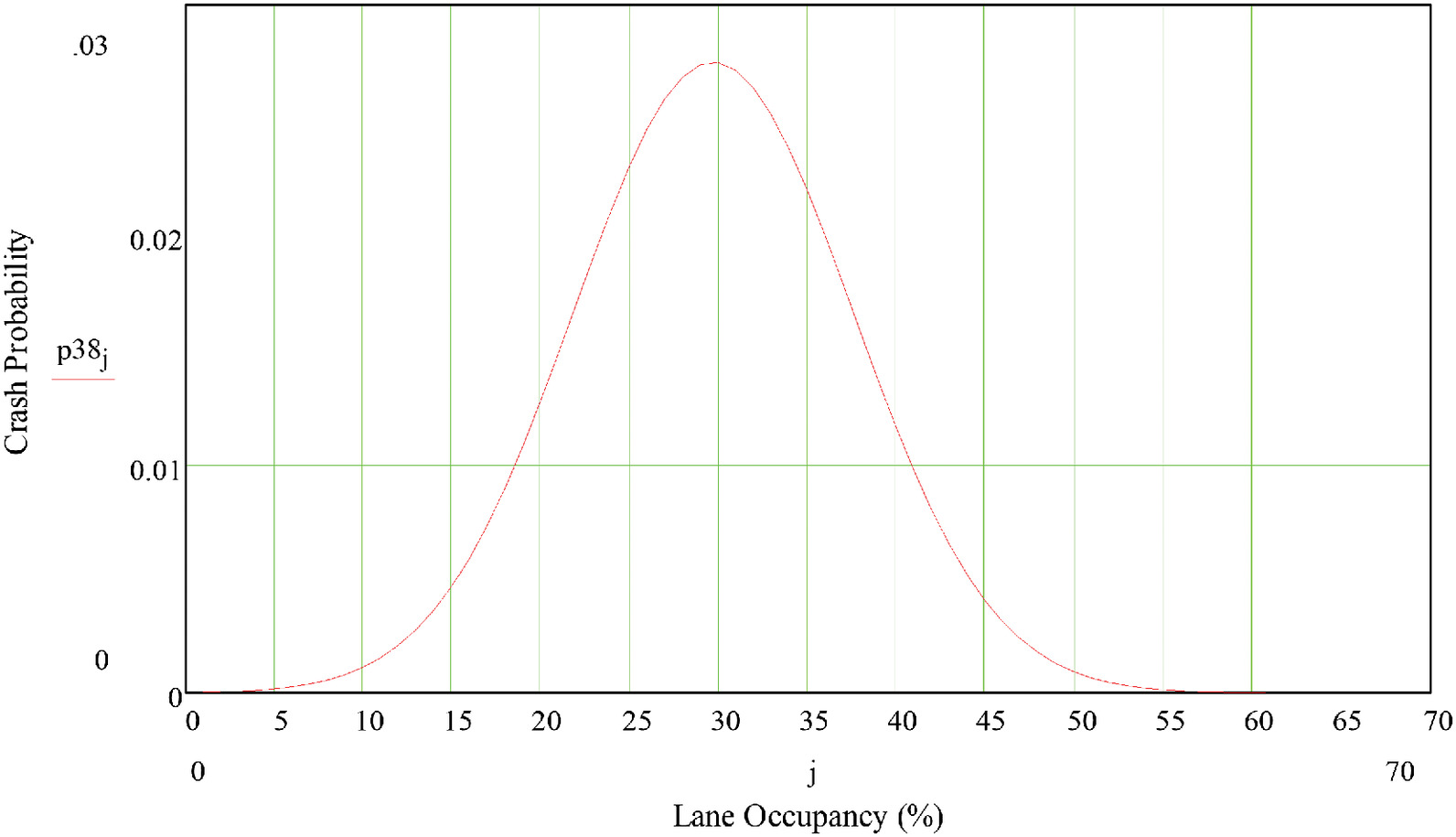
Fig. 3 shows the relationship between lane occupancy and rear-end crash risk, as predicted by the logit model summarized in Table 1. Taking the derivative of Eq. (2) with respect to lane occupancy, setting this equal to zero, and solving for lane occupancy gives an expression for the point where crash risk was greatest. Using the estimates from Table 1, for segment N38 the crash probability was greatest when lane occupancy (%) was approximately equal towhere = average lane occupancy over all hours in the study period, which for N38 was equal to 7.26%.
(3)
Similar patterns, with rear-end crash risk showing an inverted U-shaped relationship to lane occupancy, were found for segments N37 and N40 as well as for four of five additional segments on I35W. Since lane occupancy is roughly proportional to traffic density, these results indicated that rear-end crash risk should also show an inverted U-shaped relation to traffic density.
Mechanism-Based Model of Rear-End Crash Risk
Rear-End Crashes and Stopping Waves
In this section, we describe a mechanism that predicts inverted U-shaped relations between traffic density and rear-end crash risk. Our mechanism has two main components, a fundamental diagram relating traffic flow and mean speed to traffic density, and a random walk model, originally due to Brill (1972), describing how stopping waves can lead to crashes. Our development draws substantially on analytic and empirical work described in Chatterjee’s (2016) Ph.D. thesis.
For the logistic regression model summarized in Table 1, the estimates of and summarize the statistical associations between lane occupancy and rear-end crash risk, but only for the roadway and driver/vehicle population that generated our data. Assessing the model’s transferability (i.e., its external validity) still involves determining if “the mechanism responsible for B in the target population is sufficiently similar to that responsible for B in the study population” (Parkkinen et al. 2018), and this requires insight into the relevant mechanism. Fortunately, research on the etiology of freeway rear-end crashes has been reported. Using loop-detector data, Zheng et al. (2010) found that traffic oscillations, i.e., the quasi-periodic rise and fall of traffic speeds and densities due to shockwaves, were associated with increased crash risk. Hourdos (2006) and Hourdos et al. (2006) placed video cameras on high-rise buildings overlooking a segment of Interstate-94 (I-94) in Minneapolis, identified crash and near-crash events visually, and found that upstream-propagating stopping waves were precursors to most rear-end crashes.
Stopping waves tend to be crash precursors, and stop-start waves are characteristic of level-of-service F traffic flow, but the findings from our PDSL study and those by Xu et al. (2014) suggest that waves occurring in high-density conditions might be more benign than those occurring when traffic flow is near capacity. This leads to the question of determining why a stopping wave does or does not result in a crash, and interestingly, over 40 years ago, Brill (1972) described a microscopic model for how stopping waves might produce crashes. Brill began by considering a platoon of vehicles, all traveling at the same speed, but with possibly different spatial separations. The platoon leader brakes to a stop with a deceleration , and after a reaction time , the first follower brakes to a stop at the minimum deceleration needed to avoid a collision. The second follower needs a reaction time to react after the first follower begins braking and then also brakes with the minimum deceleration needed to avoid a collision, and so on. A collision occurs between vehicles and if the deceleration needed to stop vehicle before colliding exceeds a maximum feasible value .
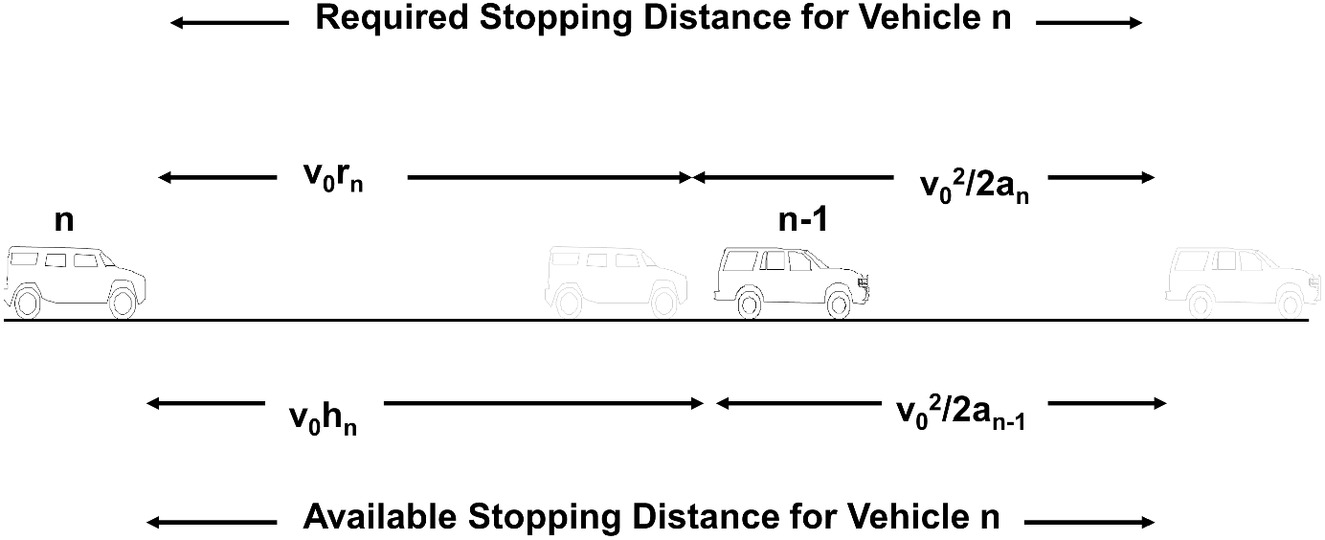
Fig. 4 illustrates the interaction between vehicles and in a stopping wave, where all vehicles have a common speed . The distance available for driver to safely stop consists of the braking distance used by preceding driver together with ’s following distance, which is the product of ’s speed and following time . The distance required by driver to stop consists of the distance traveled during ’s reaction time () plus ’s braking distance (). Fig. 4 shows driver ’s reaction time equaling the following time () so that ’s minimal successful braking rate equals ’s braking rate (). Note though that had driver ’s reaction time exceeded ’s following time (), driver would have begun braking at a point past where began braking and so would have had to brake harder in order to stop before colliding. Since implies , this in turn decreases the stopping distance available to driver compared to that for .
Brill showed that key features governing crash occurrence were the differences between drivers’ reaction times and their following times and that the cumulative contribution to crash risk made by a string of drivers could be expressed as the sum of these differences. For the case where all drivers are traveling at the same speed , a crash occurs between driver and driver when the sum of the reaction time/following time differences exceeds a critical time determined by , , and . More particularly, a crash occurs whenwhere = critical time; = braking reaction time of the th driver in the stopping wave; = following time of the th driver; = common initial speed of vehicles in the wave; = braking deceleration of the lead driver; and = maximum feasible braking deceleration.
(4)
Treating the time differences as independent random variables, Brill pointed out that the sum was a random walk and that the probability of a crash first occurring between vehicles and was related to the random walk’s first passage. Brill showed that if the mean differences between drivers’ reaction times and their following times were positive, i.e., , then a crash somewhere in an infinitely-long stopping wave was inevitable. He also derived an upper bound for the crash probability when this difference was negative, .
Empirical support for Brill’s idea can be found in the literature. Davis and Swenson (2006) used video recordings of three crash-producing stopping waves to estimate speeds, reaction times, following times, and braking rates for individual drivers. They found a definite tendency for reaction times to exceed following times so that Brill’s model of progressively more severe braking explained the occurrence of these crashes. Chatterjee (2016) and Chatterjee and Davis (2016) extended Eq. (4) to allow for variability in vehicle speeds, producing a crash condition based on a critical distancewhere = speed of vehicle ; and = common separation distance between a vehicle’s rear and its follower’s front when stopped.
(5)
To test the relationship shown in Eq. (5), Chatterjee investigated video recordings of 51 stopping waves seen in the rightmost lane of a segment of I-94 near downtown Minneapolis. Five of these waves resulted in crashes, 35 were braking-to-stop events that did not result in crashes within the segment under view, and 11 resulted in near-crashes where drivers avoided collisions by swerving out of the lane. Vehicle trajectory data, extracted from the videos, were used to estimate individual speeds, reaction times, following times, and braking rates. All 35 noncrash stopping waves failed to satisfy the crash sufficiency condition in Eq. (5), and all 11 of the swerving events would have satisfied the condition had the drivers not swerved. Three of the five crashes also satisfied condition (5), with one of the undetected crashes involving a driver making a sudden lane-change into a lane of slower-moving traffic and then rear-ending a leading vehicle, while the other involved an apparent distraction where the rear-ending driver showed no evidence of reaction or deceleration before the collision.
Relating Crash Risk to Traffic Density
The crash conditions presented in Eqs. (4) and (5) depend on drivers’ reaction times, speeds, and following times. The following times depend on vehicle speeds and separation distances, which in turn depend on traffic density. Observations have shown that mean vehicle speeds are related to traffic densities, and elementary traffic flow theory provides several models, such as Greenshield’s (1935) linear model or one based on Newell’s (1993) triangular fundamental diagram, that can be used to approximate steady-state speed-density and flow-density relationships. In these models, increases in traffic density lead to decreases in vehicles’ separations and speeds, the overall effect being that the relationship between traffic flow and traffic density shows a roughly concave shape, with a maximum flow occurring at what is commonly called the critical density. Mean following time, i.e., the time between when the rear of a leading vehicle crosses a point and when the front of the following vehicle crosses that same point, then depends on both traffic density and flow according to the relationwhere = following time; = vehicle length; = traffic density; and = traffic flow as a function of traffic density.
(6)
Fig. 5 plots Eq. (6) for a single freeway lane, where the steady-state flow/density relation follows Newell’s triangular fundamental diagram with a capacity flow of 2,250 vehicles/hour/lane, a free-flow speed of (55 mi/h), and a wave speed of (15 mi/h). The relationship between mean speed and density is given by = free-flow speed; = wave speed; = density of maximum traffic flow; and = jam density.
(7)
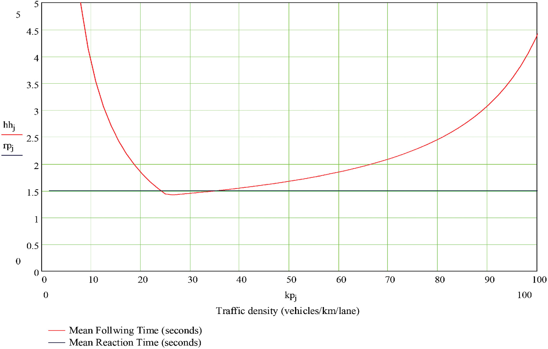
The common vehicle length for Fig. 5 was taken to be (15 ft).
Also shown in Fig. 5 is a horizontal line corresponding to a mean reaction time of 1.5 s. As can be seen, for most traffic densities, the mean following time exceeds this mean reaction time. The corresponding random walks in Eq. (5) have negative drift, and Brill’s model tells us that the probability of a crash even for infinitely-long platoons can be less than 1.0. However, for densities between about and , the mean reaction time is longer than the following time; the associated random walks then show positive drift and crashes become inevitable for arbitrarily long platoons.
Brill’s results apply to infinitely-long platoons. Similar results for the finite platoons that one might expect to see on roads require probability distributions for the first passages of random walks, which can be difficult to come by and usually involve recursively solving sequences of integral equations (Redner 2001; Champ and Rigdon 1991). Chatterjee (2016) addressed this problem by adapting an approximation developed by Brook and Evans (1972) where the continuous state space for was approximated by a discrete, finite set, and the resulting discrete random walk was modeled as an absorbing Markov chain. Crashes corresponded to the absorbing state for this Markov chain, and well-known results for finite Markov chains could be used to compute crash probabilities. This computational procedure is illustrated in the Appendix and can be adapted to relate crash risk to traffic density, as follows:
(0) Begin with a fixed length of road , a vehicle length , an initial deceleration , and a maximum deceleration . Also required are parameters for a steady-state speed-density relationship and a probability distribution for drivers’ reaction times.
1.
2.
From , , and , compute the critical time ).
3.
Divide the interval (, ) into subintervals. The midpoints of the subintervals correspond to discrete values for . Augment these with the intervals (, ) and (, ).
4.
Using the probability distribution for the reaction times compute state transition probabilities for the discrete random walk over the states defined in step (3), with the state (, ) being an absorbing state.
5.
If R denotes the submatrix containing the transition probabilities among the Markov chain’s non-absorbing states then the probabilities of collisions, from each of the initial states, are the elements of the vectorwhere denotes a vector with each element equal to 1.0. The element of corresponding to the starting state is the desired collision probability.
(8)
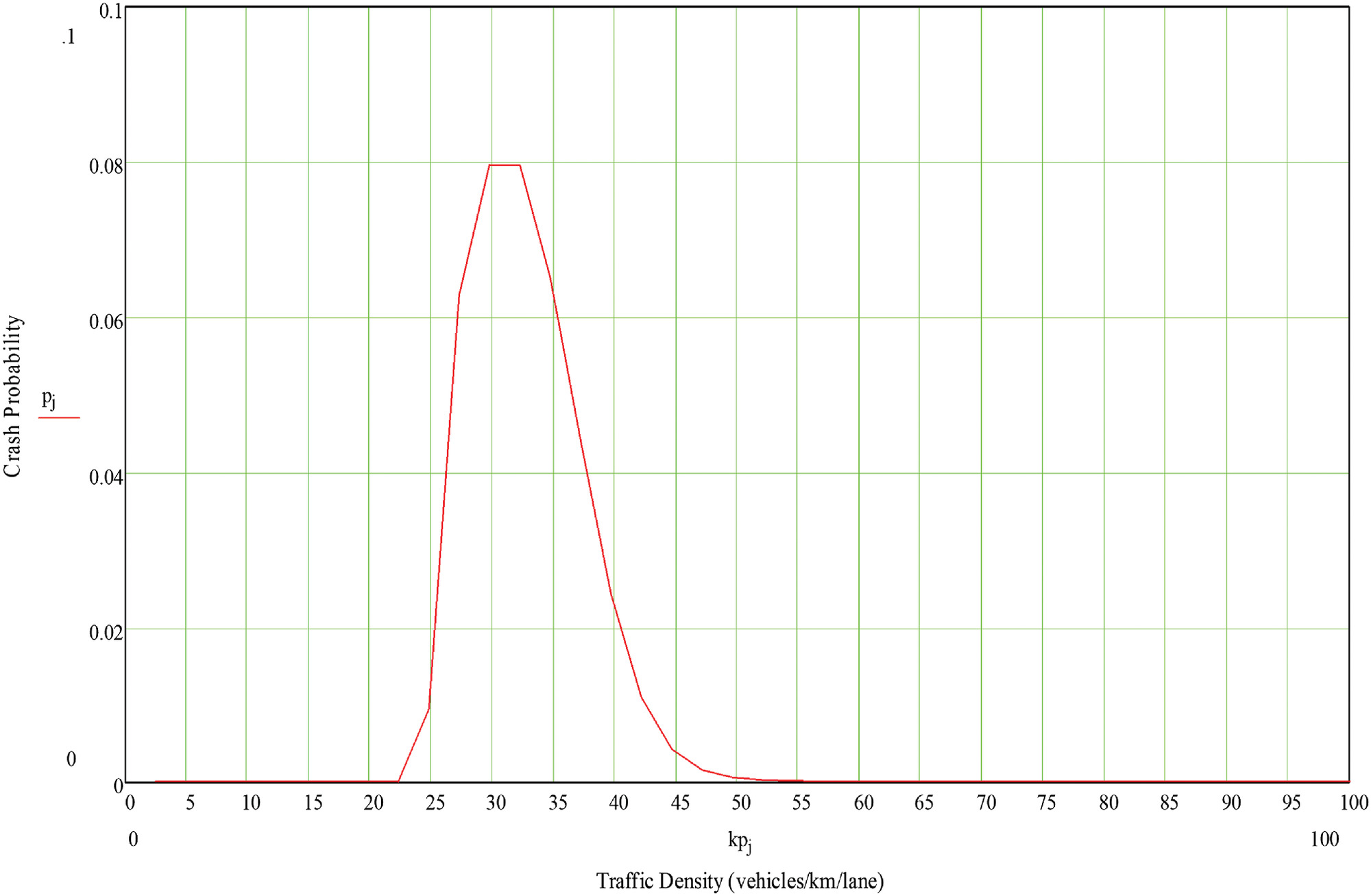
Fig. 6 shows the resulting relationship between crash probability and traffic density corresponding to Fig. 5. Driver reaction times were taken to be normally distributed with a mean of 1.5 s and a standard deviation of 0.2 s. The maximum risk of about 0.08 occurs when traffic density is about () and decreases for traffic densities above and below this point. The graph in Fig. 6 was developed using discrete states.
Testing the Random Walk Model
Before describing an empirical test of the modified Brill’s model, three points need to be considered. First, from a practical standpoint, Brill’s model is better viewed as describing potential crashes, i.e., events where braking is insufficient to avoid collisions, rather than rear-end crashes per se. As noted, when braking alone will not prevent a crash, a driver can sometimes avoid collision by swerving into an adjacent lane or onto a shoulder. This implies that model predictions should be compared to both crashes and near-crashes, where near-crashes are defined as events where drivers avoid collision by swerving. Second, so far, the model relates the probability of a crash/near-crash event to traffic density and to the occurrence of a stopping wave, (crash/near-crash | wave & density). To compare the model to empirical results, we need to consider that the likelihood of stopping waves might also vary with traffic conditions. That is, since in our model stopping waves are necessary for rear-end crashes, what we need is (crash/near-crash | wave & density) (wave | density). Ideally, a model for (wave | density) could be derived by considering drivers’ car-following behavior, and both analytic and field studies suggest that stopping waves arise from instabilities in drivers’ car-following (Wilson and Ward 2011; Stern et al. 2018). At this time, though determining which of an array of car-following models best describes driver behavior is an open question, and an empirical approach to modeling (wave | density) has more short-run promise. Third, there is evidence that drivers’ reaction times and following behavior are not independent, with drivers tending to show shorter reaction times when spacings are shorter (e.g., Chen et al. 2014). This tendency should be allowed for.
Regarding the relationship between traffic density and shockwave occurrence, video and loop-detector data were compiled by Chatterjee (2016) for the right-hand lane of a 411.5 m (1,350 ft) segment of westbound I-94. From the loop-detector data, parameters for Newell’s model were estimated, giving a free-flow speed of (55 mi/h), a critical density of (), and a wave speed (11.3 mi/h). The period between 10 a.m. and 6 p.m. was divided into 15-min intervals, and Chatterjee (2016) showed that the probability of a crash/near-crash occurring during a 15-min interval can be expressed aswhere = probability of crash/near-crash during a 15-min interval; = basic time interval during which at most one shockwave can occur; = probability a shockwave produces a crash/near-crash; = probability of a shockwave occurring during a basic time interval; and = number of basic intervals during a 15-min period.
(9)
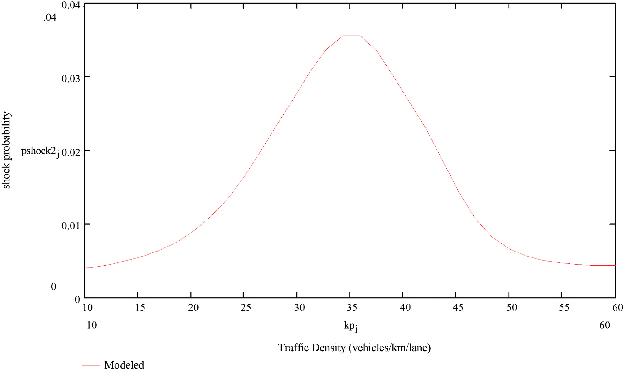
For a given traffic density, can be computed using Brill’s random walk model. To develop a relationship between and traffic density, loop-detector data were used to identify when waves producing speed reductions of (15 mi/h) or greater had occurred, on each of 83 weekdays, during the spring and summer of 2013. Using a basic interval , that being approximately the time needed for a wave to traverse the study segment at the estimated wave speed, the shockwave counts were used to compute empirical estimates of for each 15-min interval between 10 a.m. and 6 p.m. For example, between 10:00 and 10:15, five shockwaves were observed over the 83 weekdays, and using , the empirical estimate of for 10:00–10:15 was . This value for was then paired with the average traffic density between 10:00 and 10:15 over the 83 weekdays, (). Applying kernel regression to the empirical estimates of the shock probabilities and their corresponding average traffic densities gave the nonparametric relationship between traffic density and probability of shockwave occurrence shown in Fig. 7.
Finally, as noted earlier, by using video to reconstruct the trajectories of stopping vehicles, Chatterjee (2016) estimated the following times, reaction times, speeds, and braking rates for drivers in 55 waves. One finding was that drivers’ reaction times depended on their following times, with those having shorter following times also tending to have shorter reaction times. A linear regression model relating reaction time to the following time producedwith the standard deviation for the random errors being 0.54.
(10)
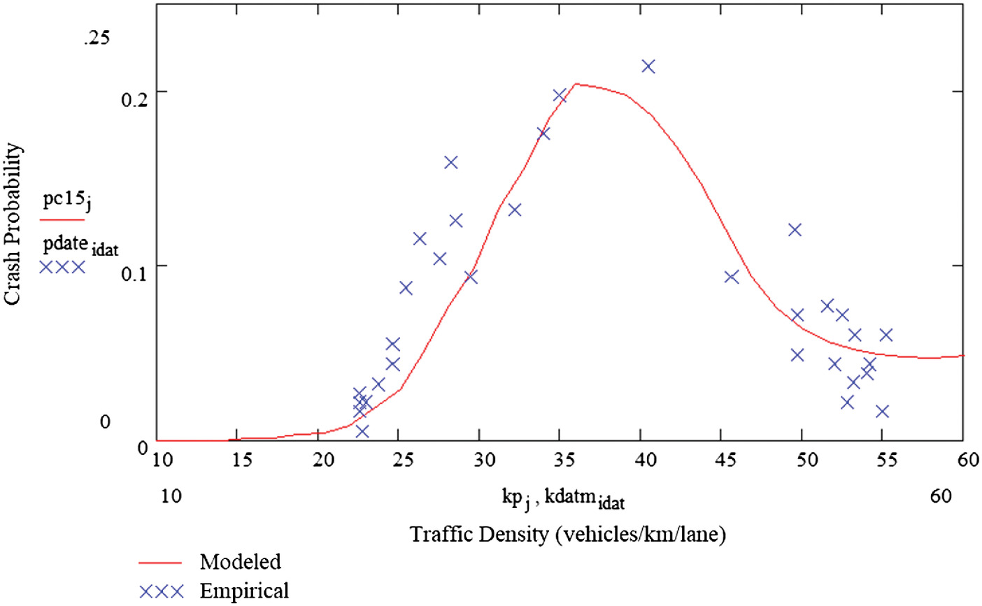
Chatterjee also reviewed crash/near-crash data collected by the Minnesota Traffic Observatory during 2012–2013 and from this computed empirical estimates of the probability of a crash/near-crash occurring during each 15-min interval between 10 a.m. and 6 p.m. A predicted probability of a crash/near-crash occurring during a 15-min interval, as a function of traffic density, was then computed using Eq. (9) by combining the nonparametric regression model shown in Fig. 7, the regression model relating reaction time to following time [Eq. (10)], the fitted version of Newell’s model, and Brill’s random walk model as approximated by a finite Markov chain. Fig. 8 shows the empirical crash probabilities taken from Chatterjee’s (2016, p. 75) Figure 4.15 plotted against average traffic density, along with the predicted crash/near-crash probabilities computed by the combined model. The initiating and maximum decelerations, meters per second ( [7.4 feet per second ] and , respectively, were also taken from Chatterjee’s video-based estimates. Fig. 8 shows a reasonable correspondence between the measured and modeled probabilities of crash/near-crash events. The probability relation shows an inverted U-shape, with maximum risk occurring between 34 and .
Transferring Knowledge to an AV Environment
The logistic regression model illustrated in Fig. 3 summarized the association between crash risk and lane occupancy for drivers and vehicles present during 2004–2013. As noted earlier, though, transferring this model to a population of AVs is problematic. Fig. 6, on the other hand, shows the probability that a stopping wave produces a crash or near-crash event and was developed from a mechanism-based model, where a fundamental diagram described steady-state car-following behavior and where Brill’s random walk model described how a stopping wave leads to a crash or near-crash event. In principle, a fundamental diagram describing traffic flow for AVs, along with data on their braking rates and reaction times, should make it possible to construct a similar diagram for the AVs. In what follows, we illustrate how this can be done for a population of AVs equipped with ACC and AEB. All vehicles in our hypothetical population are assumed to have the same ACC and AEB systems. Car-following is assumed to be governed by the ACC system while braking in a stopping wave is governed by the AEB system. Estimates from recently conducted field studies of ACC and AEB systems currently on the road are then used to characterize crash risk in a hypothetical platoon of AVs.
Regarding AEB, researchers have recently conducted field tests of a system implemented in two 2017 Toyota Corollas (Yang et al. 2018; Xing et al. 2018). This system used radar mounted behind the front grill and a monocular camera mounted just in front of the rear-view mirror to identify possible hazards. The system issued auditory and visual alarms when predicted time-to-collision fell below a threshold; if the driver did not respond, or if the driver’s response appeared insufficient to prevent the collision, the system initiated full braking autonomously. In the field tests, the timing of these and related events were obtained from the system’s vehicle control history (VCH). The tests involved approaching a stationary object with a constant accelerator pedal position and no braking by the driver and then recording the vehicle’s final position along with data from the VCH. Xing et al. (2018, p. 5) noted that autonomous deceleration appeared to correlate with an event labeled FPB in the VCH, while Yang et al. (2018, p. 5) noted that the average time between the warning and the start of autonomous deceleration was approximately 0.94 s. They also reported a maximum braking rate deceleration of and suggested that a plausible standard deviation for the time lag between the warning signal and the start of deceleration was 0.12 s. Adding 0.1 s to account for the time needed by the system to identify a hazard gave the following characteristics for our hypothetical AEB system: mean reaction time , reaction time standard deviation , and maximum braking rate .
Regarding ACC, field experiments seeking to characterize the car-following behavior of existing ACC systems have been described in Gunter et al. (2019a, b). These involved recording the positions of leading and following vehicles during car-following situations where the following vehicles were operating under ACC. Parameters characterizing different car-following models were then estimated by minimizing the squared error between observed and predicted speed histories for seven different vehicle models. Gunter et al. (2019b, p. 3053) compared three different car-following models and concluded that the optimal velocity with relative velocity term (OVRV) model and the intelligent driver model (IDM) “perform roughly the same.” Gunter et al. (2019a) fit OVRV models to data from the seven vehicle models and then used stability analysis methods to assess the string stability of the estimated car-following behavior. Interestingly, the authors found that the fitted models for each of the seven ACC systems were string unstable, i.e., they tended to amplify disturbances and so, potentially, could generate stopping waves. Recognizing that replication and extension of this pioneering work is needed before conclusions can be finalized, we will use some of these results to illustrate how the model developed in in the section “Mechanism-Based Model of Rear-end Crash Risk” might be transferred to an AV environment.
The version of the OVRV model used in Gunter et al. (2019a) has as its steady-state relationship between mean traffic speed and traffic density = ACC’s target time headway; and = jam spacing, and this is a version of the right-hand side () of Newell’s model shown in Eq. (7). For a given free-flow speed , the corresponding wave speed and critical density can be computed via
(11)
(12)
Gunter et al. (2019a) fit separate models for when the vehicles’ ACCs were at their minimum (shortest headway) and maximum (longest headway) settings. For their vehicle A at the minimum setting, the estimated target headway was and the estimated jam spacing was , while at the maximum setting, the estimated parameters were and . For our hypothetical AV, we used estimates for both settings to construct fundamental diagrams, in each case with a free-flow speed of (55 mi/h).
Fig. 9 shows the steady-state following times for vehicle A at both its minimum and maximum settings. Also shown is the mean reaction time for the AEB system, 1.04 s. For the minimum setting, the mean following time is generally longer than the mean braking reaction time, but it dips below the mean reaction time when traffic density is roughly between 33 vehicles/km/lane and 45 vehicles/km/lane. Brill’s model then tells us that for traffic densities in this range, and for long platoons, a stopping wave is likely to result in a crash. At the maximum setting, however, the steady-state mean following time is never below 2.0 s, suggesting that stopping waves would most likely be benign.
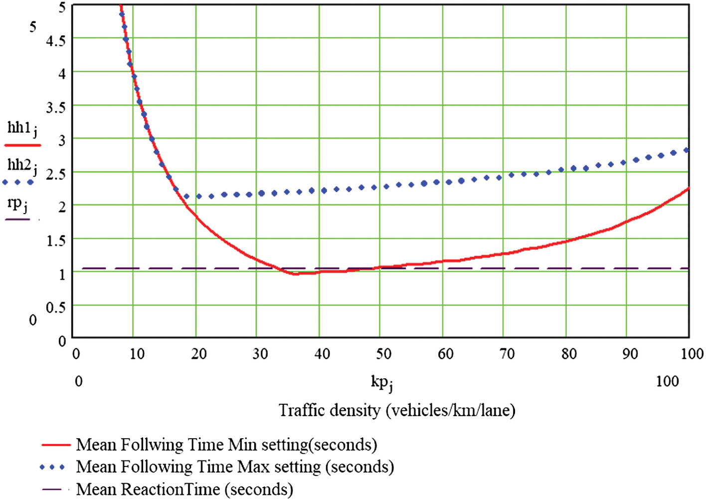
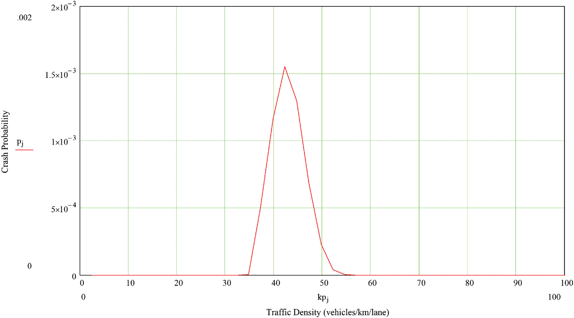
Fig. 10 shows the probability a stopping wave produces a crash/near-crash in a 0.4 km (0.25 mi) long section of one freeway lane. Car-following and braking behavior were the same as those for the model A vehicle at its minimum setting, and the initiating deceleration was, as for Fig. 6, (). Crash probabilities were computed using the finite Markov chain approximation described in the section “Mechanism-Based Model of Rear-End Crash Risk.” The greatest risk occurs at densities of approximately 43 vehicles/km/lane. For the ACCs at the maximum setting, on the other hand, all computed crash probabilities were less than .
Summary and Conclusion
Using data from I-35W in Minneapolis, empirical logistic regression analyses found inverted U-shaped relationships between crash risk and lane occupancy. Macroscopic traffic flow models imply that vehicle headways should show a roughly convex relation to traffic density; headways tend to be long when densities are low because vehicles are widely separated, and headways tend to be long when densities are high because vehicles have slow speeds. Brill’s microscopic model of how a platoon of braking vehicles can produce a rear-end crash emphasizes the differences between reaction times and following times and shows how the probability of a crash occurring in a stopping wave can be computed via the first passage of a random walk. By combining Brill’s model with a macroscopic traffic flow model, it was possible to predict a relationship between traffic density and rear-end crash risk. Computational difficulties related to passage times for random walks were alleviated by approximating the random walks with finite Markov chains. The resulting combined model predicted an inverted U-shape to the relation between traffic density and the probability that a stopping wave produced a crash/near-crash. Although it is not yet clear how to transfer empirical regression models, such as the HSM’s SPF, to situations where AVs are present, it is possible to transfer the mechanism-based model described in the “Mechanism-Based Model of Rear-End Crash Risk” section. This possibility was illustrated using data from field tests of vehicles equipped with ACC and AEB.
Our findings should be regarded as promising rather than final. What we have presented is an example of how a mechanism-based model can (1) relate crash risk to traffic conditions and (2) be transferred to an environment containing AVs. The empirical support for our model came from detailed study of one section of I-94, so replication using other freeway sections is needed. Also, our model has four main components: a steady-state relationship between traffic density and mean speed, a probability model for drivers’ reaction times, a random walk model describing how a stopping wave produces a rear-end crash, and an empirical model relating traffic density to the probability that a stopping wave occurs. It is possible that, with additional work, each of these component models could be replaced. In particular, the random walk in Eq. (4) could be replaced by a more detailed stochastic process that allows vehicles/drivers in a wave to have different speeds, braking strategies, or reaction models, while the empirical relationship between traffic density and stopping wave probability could, in principle, be replaced by one derived from car-following theory. Research into the capabilities of AVs is at an early stage and undoubtedly the ACC and AEB models described in the “Transferring Knowledge to an AV Environment” section can, and probably will, be replaced in the future. In the near term, it will also be important to consider traffic with mixtures of AVs and legacy vehicles. We would also like to note that while the model presented here does not include infrastructure-related features, recent work has illustrated how mechanism-based modeling can explain CMFs associated with changes in left-turn lane offset (Davis 2021) and installation of pedestrian hybrid beacons (Davis 2019). The challenge here is not so much model construction as it is our limited understanding of how crash-related modifications achieve their effects.
Finally, Brill’s model is a hypothesized mechanism for explaining how rear-end crashes occur. This contrasts with the statistical models that underpin the HSM, which can produce useful results even when little is known about how crashes occur. An ongoing debate concerns the value of mechanistic models and explanations for highway safety engineering (Bonneson and Ivan 2013), and interestingly, there is a similar debate about the role of mechanisms in evidence-based medicine (Howick 2011). Proponents of evidence-based medicine generally regard randomized controlled trials as providing the strongest evidence for the effectiveness of treatments, and an open question concerns what role knowledge of physiological mechanisms should play in prescribing treatments (Andersen 2012). Bluhm (2013) has argued that mechanistic knowledge in medical research could be used to guide and focus the design of statistical studies, and something similar occurred in our I-35W study (Davis et al. 2017). Brill’s mechanism, coupled with Greenshield’s fundamental diagram, was used to suggest the quadratic form for lane occupancy predictors in the logistic regressions, leading to noticeable improvements in model fit. More generally, in addition to guiding decisions about external validity, the heuristic value of mechanisms for suggesting productive lines of research should not be discounted.
Notation
The following symbols are used in this paper:
- vector with all elements equal to 1.0;
- braking deceleration of the lead driver;
- maximum feasible braking deceleration;
- common separation distance between vehicles;
- traffic density;
- density of maximum traffic flow;
- jam density;
- driver following time;
- effective vehicle length;
- vehicle length;
- lane occupancy;
- probability of crash/near-crash during a 15-min interval;
- probability of a shockwave during an interval of ;
- probability a shockwave results in a crash/near-crash;
- traffic flow;
- R
- submatrix of transition probabilities;
- driver braking reaction time;
- critical time;
- ACC target time headway;
- common initial speed of vehicles in the wave;
- speed of vehicle ;
- free-flow speed;
- wave speed;
- row of logistic regression independent variable matrix;
- occurrence/nonoccurrence of a crash;
- ,
- logistic regression parameters;
- ACC jam spacing; and
- vector of crash probabilities.
Appendix. Computing Crash Probabilities
In the section “Mechanism-Based Model of Rear-End Crash Risk,” we approximated the random walk in Eq. (5) with a finite, discrete-state Markov chain. Derivations of this approximation have been given elsewhere (Brook and Evans 1972, p. 543; Chatterjee 2016, pp. 59–61); here, we simply illustrate how the approximation is constructed. Consider one lane in a 0.4 km (0.25 mi) segment of freeway, where the traffic is well-described by Newell’s model with a capacity flow of 2,250 vehicles/hour/lane, a free-flow speed of (55 mi/h), and a wave speed of (15 mi/h). Driver reaction times are normally distributed, with a mean of 1.5 s and a standard deviation of 0.2 s, and the maximum feasible braking rate is (). In the lane of interest, traffic density is currently () when a driver at the segment’s downstream boundary brakes to a stop at (). Newell’s model with the above parameters, and the given traffic density, gives the common speed in this lane as mps (), and there are vehicles in this lane. The common following time is then , and the critical time is .
To illustrate the computation of the Markov chain’s transition probabilities, we will, unrealistically, approximate the state space for using only states. The range () is first divided into intervals of width . The absorbing state is given index 5 and corresponds to the crash condition . State 1 corresponds to , while states 2, 3, and 4 represent intermediate values for . State 3, with a midpoint of 0 s, represents between and , while state 4 has a midpoint of 0.8 s and represents between 0.4 and 1.2 s. A transition from state 3 to state 4 occurs when the reaction time/following time difference , plus the midpoint of state 3, is greater than the lower boundary for state 4 but not greater than the upper boundary of state 4. For this example, would need to be greater than 0.4 s, so that , but less than 1.2, so that . Since is assumed to be normally distributed, with a mean of 1.5 s and a standard deviation of 0.2 s, while is constant at 1.52 s, we have . Table 2 shows the resulting transition matrix P for this five-state approximation to . Here , leading to the mild negative drift shown in the transition matrix.
| Starting state (midpoint) | Ending state (midpoint) | ||||
|---|---|---|---|---|---|
| 1 () | 2 () | 3 (0) | 4 (0.8) | 5 (1.6) | |
| 1 () | 0.982 | 0.018 | 0 | 0 | 0 |
| 2 () | 0.029 | 0.953 | 0.018 | 0 | 0 |
| 3 (0) | 0 | 0.029 | 0.953 | 0.018 | 0 |
| 4 (0.8) | 0 | 0 | 0.029 | 0.953 | 0.018 |
| 5 (1.6) | 0 | 0 | 0 | 0 | 1 |
Taking the submatrix consisting of the first four rows and columns of this matrix to be the matrix R in Eq. (8) and letting be the number of vehicles in this lane, we have
(13)
The probability that this stopping wave produces a crash would then be 0.022. In practice, a finer discretization of the state space should be used, and in our experiments, resulted in collision probabilities that were stable to four decimal places. Computing the probabilities shown in Figs. 6, 8, and 10 was done using Mathcad (e.g., Maxfield 2009), and copies of this Mathcad document are available from the corresponding author upon reasonable request.
Data Availability Statement
Some or all data, models, or code that support the findings of this study are available from the corresponding author upon reasonable request.
Acknowledgments
This research was supported in part by the Minnesota DOT. The authors would like to thank Raphael Stern for his insight and guidance regarding the ACC models in the section “Transferring Knowledge to an AV Environment.”
References
AASHTO. 2010. Highway safety manual. Washington, DC: AASHTO.
AASHTO. 2017. A policy on geometric design of highways and streets. Washington, DC: AASHTO.
Abdel-Aty, M., A. Pande, M. Abdalla, N. Uddin, and L. Hsia. 2004. “Predicting freeway crashes from loop detector data by matched case-control logistic regression.” Transp. Res. Rec. 1897 (1): 88–95. https://doi.org/10.3141/1897-12.
Andersen, H. 2012. “Mechanisms: What are they evidence for in evidence-based medicine?” J. Eval. Clin. Pract. 18 (5): 992–999. https://doi.org/10.1111/j.1365-2753.2012.01906.x.
Bluhm, R. 2013. “Physiological mechanisms and epidemiological research.” J. Eval. Clin. Pract. 19 (3): 422–426. https://doi.org/10.1111/jep.12035.
Bonneson, J., and J. Ivan, eds. 2013. “Theory, explanation, and prediction in road safety: Promising directions.” In Research circular E-C179. Washington, DC: Transportation Research Board.
Brill, E. A. 1972. “A car-following model relating reaction times and temporal headways to accident frequency.” Transp. Sci. 6 (4): 343–353. https://doi.org/10.1287/trsc.6.4.343.
Brook, D., and D. Evans. 1972. “An approach to the probability of cusum run length.” Biometrika 59 (3): 539–549. https://doi.org/10.1093/biomet/59.3.539.
Campbell, D., and J. Stanley. 1966. Experimental and quasi-experimental designs for research. Chicago: Rand-McNally.
Cartwright, N., and J. Hardie. 2012. Evidence-based policy: A practical guide to doing it better. Oxford, UK: Oxford University Press.
Champ, C., and S. Rigdon. 1991. “A comparison of the Markov chain and the integral equation approaches for evaluating the run length distribution of quality control charts.” Commun. Stat.-Simul. Comput. 20 (1): 191–204. https://doi.org/10.1080/03610919108812948.
Chatterjee, I. 2016. “Understanding driver contributions to rear-end crashes on congested freeways and their implication for future safety measures.” Ph.D. dissertation, Dept. of Civil, Environmental, and Geo-Engineering, Univ. of Minnesota Digital Conservancy.
Chatterjee, I., and G. Davis. 2016. “Analysis of rear-end events on congested freeways by using video-recorded shockwaves.” Transp. Res. Rec. 2583 (1): 110–118. https://doi.org/10.3141/2583-14.
Chen, D., S. Ahn, J. Lava, and Z. Zheng. 2014. “On the periodicity of traffic oscillations and capacity drop: The role of driver characteristics.” Transp. Res. Part B 59 (Jan): 117–136. https://doi.org/10.1016/j.trb.2013.11.005.
Davis, G. 2019. “Explaining crash modification factors: Why its needed and how it might be done.” Accid. Anal. Prev. 131 (Oct): 225–233. https://doi.org/10.1016/j.aap.2019.06.015.
Davis, G. 2021. “Transferability of crash modification factors via graphical causal models: Application to sight distance and left-turn lane offsets.” In Proc., Presented at 2021 Annual Meeting. Washington, DC: Transportation Research Board.
Davis, G., J. Gao, and J. Hourdos. 2017. Safety impacts of the I-35W improvements done under Minnesota’s urban partnership agreement (UPA) project. St. Paul, MN: Minnesota DOT.
Davis, G. A., and T. Swenson. 2006. “Collective responsibility for freeway rear-end accidents?: An application of probabilistic causal models.” Accid. Anal. Prev. 38 (4): 728–736. https://doi.org/10.1016/j.aap.2006.01.003.
FHWA (Federal Highway Administration). 2015. Crash modification factors needs assessment workshop. Washington, DC: FHWA.
Garber, N. J., and L. A. Hoel. 2015. Traffic and highway engineering. 5th ed. Stamford, CT: Cengage Learning.
Greenshields, B. D., W. Channing, and H. Miller. 1935. “A study of traffic capacity.” In Vol. 14 of Proc., Highway Research Board, 448–477. Washington, DC: National Research Council.
Gunter, G., et al. 2019a. “Are commercially implemented adaptive cruise control systems string stable?” Accessed November 5, 2019. https://arxiv.org/abs/1905.02108.
Gunter, G., R. Stern, and D. Work. 2019b. “Modeling adaptive cruise control vehicles from experimental data: Model comparison.” In Proc., 2019 IEEE Intelligent Transportation Systems Conf., 3049–3054. New York: IEEE.
Haus, S., R. Sherony, and H. Gabler. 2019. “Estimated benefit of automated emergency braking systems for vehicle-pedestrian crashes in the United States.” Supplement, Traffic Inj. Prev. 20 (S1): S171–S176. https://doi.org/10.1080/15389588.2019.1602729.
Hourdos, J. 2006. “Crash prone traffic flow dynamics: Identification and real-time detection.” Ph.D. dissertation, Dept. of Civil Engineering, Univ. of Minnesota.
Hourdos, J. N., V. G. Garg, P. A. Michalopoulos, and G. Davis. 2006. “Real-time detection of crash-prone conditions at freeway high-crash locations.” Transp. Res. Rec. 1968 (1): 83–91. https://doi.org/10.1177/0361198106196800110.
Howick, J. 2011. The philosophy of evidence-based medicine. Chichester, UK: Wiley.
Illari, P., and J. Williamson. 2012. “What is a mechanism: Thinking about mechanisms across the sciences.” Eur. J. Philos. Sci. 2 (1): 119–135. https://doi.org/10.1007/s13194-011-0038-2.
Kusano, K., and H. Gabler. 2012. “Safety benefits of forward collision warning, brake assist, and autonomous braking systems in rear-end collisions.” In Vol. 13 of Proc., IEEE Transactions on Intelligent Transportation Systems, 1546–1555. New York: IEEE.
Lee, C., F. Saccomanno, and B. Hellinga. 2002. “Analysis of crash precursors on instrumented freeways.” Transp. Res. Rec. 1784 (1): 1–8. https://doi.org/10.3141/1784-01.
Liu, G., and A. Popoff. 1997. “Provincial-wide travel speed and traffic safety study in Saskatchewan.” Transp. Res. Rec. 1595 (1): 8–13. https://doi.org/10.3141/1595-02.
Machamer, P., L. Darden, and C. Caver. 2000. “Thinking about mechanisms.” Philos. Sci. 67 (1): 1–25. https://doi.org/10.1086/392759.
Mannering, F., V. Shankar, and C. Bhat. 2016. “Unobserved heterogeneity and the statistical analysis of highway accident data.” Anal. Method Accid. Res. 11 (Sep): 1–16. https://doi.org/10.1016/j.amar.2016.04.001.
Maxfield, B. 2009. Essential Mathcad for engineering, science, and math. 2nd ed. Burlington, MA: Academic Press.
NCHRP (National Cooperative Highway Research Program). 2019a. Assessing the impacts of automated driving systems (ads) on the future of transportation safety. NCHRP 17-91. Washington, DC: NCHRP.
NCHRP (National Cooperative Highway Research Program). 2019b. Development of crash prediction models for short-term durations. NCHRP 22-48. Washington, DC: NCHRP.
Newell, G. 1993. “A simplified theory of kinematic waves in highway traffic. Part I: General theory.” Transp. Res. Part B 27 (4): 281–287. https://doi.org/10.1016/0191-2615(93)90038-C.
Oh, C., J.-S. Oh, S. Ritchie, and M. Chang. 2001. “Real-time estimation of freeway accident likelihood.” In Proc., 80th Transportation Research Board Annual Meeting. Washington, DC: Transportation Research Board.
Parkkinen, V.-P., C. Wallman, M. Wilde, B. Clarke, P. Illari, M. Kelly, C. Norell, F. Russo, B. Shaw, and J. Williamson. 2018. Evaluating evidence of mechanisms in medicine: Principles and procedures. New York: Springer.
Redner, S. 2001. A guide to first-passage processes. Cambridge, UK: Cambridge University Press.
Rosen, E., J. Kalhammer, D. Eriksson, M. Nentwich, R. Fredriksson, and K. Smith. 2010. “Pedestrian injury mitigation by autonomous braking.” Accid. Anal. Prev. 42 (6): 1949–1957.
Roshandel, S., Z. Zheng, and S. Washington. 2015. “Impact of real-time traffic characteristics on freeway crash occurrence: Systematic review and meta-analysis.” Accid. Anal. Prev. 79 (Jun): 198. https://doi.org/10.1016/j.aap.2015.03.013.
Stern, R., et al. 2018. “Dissipation of stop-and-go waves via control of autonomous vehicles: Field experiments.” Transp. Res. Part C: Emerging Technol. 89 (Apr): 205–221. https://doi.org/10.1016/j.trc.2018.02.005.
Wilson, R., and J. Ward. 2011. “Car-following models: Fifty years of linear stability analysis-A mathematical perspective.” Transp. Plann. Technol. 34 (1): 3–18. https://doi.org/10.1080/03081060.2011.530826.
Xing, P., M. Yang, B. Tsuge, T. Flynn, J. Lawrence, and G. Siegmund. 2018. The accuracy of Toyota vehicle control history data during autonomous emergency braking. Warrendale, PA: Society of Automotive Engineers.
Xu, C., P. Liu, W. Wang, and Z. Li. 2014. “Identification of freeway crash-prone traffic conditions for traffic flow at different levels of service.” Transp. Res. Part A 69 (Nov): 58–70. https://doi.org/10.1016/j.tra.2014.08.011.
Yang, M., P. Xing, T. Flynn, B. Tsuge, J. Lawrence, and G. Siegmund. 2018. The effect of target features on Toyota’s autonomous emergency braking system. Warrendale, PA: Society of Automotive Engineers.
Zheng, Z., S. Ahn, and C. M. Monsere. 2010. “Impact of traffic oscillations on freeway crash occurrences.” Accid. Anal. Prev. 42 (2): 626–636. https://doi.org/10.1016/j.aap.2009.10.009.
Information & Authors
Information
Published In
Journal of Transportation Engineering, Part A: Systems
Volume 147 • Issue 4 • April 2021
Copyright
This work is made available under the terms of the Creative Commons Attribution 4.0 International license, https://creativecommons.org/licenses/by/4.0/.
History
Received: Mar 2, 2020
Accepted: Nov 2, 2020
Published online: Jan 27, 2021
Published in print: Apr 1, 2021
Discussion open until: Jun 27, 2021
Authors
Metrics & Citations
Metrics
Citations
Download citation
If you have the appropriate software installed, you can download article citation data to the citation manager of your choice. Simply select your manager software from the list below and click Download.