Abstract
Recently, there has been a significant amount of research related to heavy trucks operating as connected and autonomous vehicles (CAVs). As argued in this paper, to understand the potential impact on the freeway system of CAV technologies, analyses should be conducted using the standard US methodological framework. Consequently, this paper uses the exact Highway Capacity Manual, Sixth Edition (HCM-6) equal capacity passenger car equivalent (EC-PCE) methodology to estimate capacity and EC-PCEs for CAV truck platoons on freeway segments. It was found that EC-PCE values for CAV trucks are, on average, 34.3% lower compared to the values for non-CAV trucks, indicating that CAV platoons can have a positive effect on highway capacity. The amount of decrease is a function of a number of CAV operational assumptions, and these are studied through a sensitivity analysis. This paper demonstrates that the effect of CAV truck platoons can be modeled using the standard HCM-6 approach, and the methodology allows meaningful comparisons so that traffic agencies can better prepare for the adoption of CAV technologies.
Introduction
In the sixth and current version of the Highway Capacity Manual (HCM-6) passenger car equivalents (PCEs) are used to account for the effect of different vehicle types on capacity and quality of service of a mixed traffic stream. These vehicle types include heavy vehicles, motorcycles, and recreational vehicles, and the PCE accounts for differences in size and operational characteristics as compared to passenger cars. In effect, the PCE represents the number of passenger cars that would produce the same effect on the traffic flow as a given vehicle type. Transportation engineers use PCEs to convert traffic streams, measured in vehicles per hour (), to an equivalent stream that is measured in passenger car units per hour (). This allows various roadways, which have different proportions of vehicle types, to be analyzed or designed based on a single metric.
The PCE concept has been used for over in the Highway Capacity Manual (HCM) and other design guides (HCM 1965, 2016; AASHTO 2011; Urbanik et al. 2015). In the current version, HCM-6, PCEs for freeway and multilane highway segments are estimated using the equal-capacity method. The PCEs, referred to in this paper as equal capacity PCEs (EC-PCEs), are calculated using the estimated capacities of both mixed-flow and passenger car–only flow (HCM 2016; Dowling et al. 2014a; Yang 2013; Zhou 2018).
It is important to note that the HCM-6 equal capacity methodology for freeway segments is based completely on VISSIM microsimulation model results that were aggregated over intervals. The HCM-6 includes EC-PCE values for 14 levels of truck percentage, 13 levels of grade, 7 levels of grade distance, and 3 levels of truck composition type. The advantage to using a simulation model is obvious—it greatly reduces the amount of empirical data that need to be collected and allows for relatively quick analysis of many different situations. For example, on the surface it would be relatively easy to simulate connected and automated vehicles (CAVs) and use the resulting output to estimate capacity and PCE values. The disadvantages are also obvious (Hendrickson and Rilett 2017). In particular, the developers of the VISSIM model periodically update their model and do not guarantee backward compatibility. Therefore, if users are going to use later versions of VISSIM to model new situations, such as CAVs, and use the output to estimate capacity and PCE values, they must ensure that the results are compatible with the original VISSIM model used to calculate the values in the HCM-6.
Recently, there has been a significant amount of research related to heavy trucks operating as autonomous vehicles (AVs) as well as CAVs (Bujanovic and Lochrane 2018; Kang et al. 2019; Mahdavian et al. 2019). CAVs are defined as vehicles that are capable of both autonomous driving and connectivity with other entities of the transportation system (e.g., vehicles, road infrastructure) (Guanetti et al. 2018). These CAVs will form platoons where the lead vehicle “controls” the behavior of the following vehicles and the following vehicles are able to maintain time headways much smaller than that used by non-CAVs. It is hypothesized that these CAV platoons will, among other benefits, reduce congestion, increase capacity, reduce pollution, and alleviate the US commercial driver shortage. It is has been argued that heavy trucks will be the first CAVs on the national trunk highway system because the driving environment is not as complex as urban arterial networks and because there are significant benefits in terms of increased fuel efficiency, reduced operating costs, and improved truck safety (Hallmark et al. 2019; Fitzpatrick et al. 2016; Janssen et al. 2015).
It is important that the effect of CAVs on the performance of these systems be determined. While considerable work has been done on CAV modeling (Sukennik 2018; Kittelson & Associates 2019; Stanek 2019; Shi and Prevedouros 2016), no models have used the HCM-6 methodology, which is the national standard for estimating capacity and quality of service for freeways. Consequently, it is unclear exactly how the highway capacity metrics, including the HCM-6 PCE values, will need to change. This paper argues that in order to understand the potential impact on the freeway system of CAV technologies, analyses should be conducted using the standard US methodological framework. This is the motivation of this paper.
Specifically, this paper uses the exact HCM-6 EC-PCE methodology to estimate EC-PCEs for CAV trucks on freeway and multilane highway segments. The main objective is to analyze highway capacity under the interaction of CAV trucks and conventional vehicles. In addition, sensitivity analyses are conducted in order to explore the effect of four factors that are considered critical in the operation of CAVs: (1) market penetration rate, (2) lane restriction, (3) platoon truck type, and (4) platoon size. It should be noted that it is assumed that only trucks can operate in CAV mode in this study. Passenger cars will operate as conventional or non-CAVs. This assumption may be relaxed without changes to the methodology discussed in this paper. Additionally, it is assumed that the operational and geometric characteristics of the vehicles and testbeds used in the CAV analysis (e.g., acceleration/deceleration profiles, speed distributions, weight, and power distributions, vehicle lengths) are the same as those used in the original HCM-6 methodology.
The remainder of the paper is laid out in four sections. First, the current HCM-6 EC-PCE values are estimated to ensure that the current version of VISSIM can be used to replicate the existing HCM-6 values. Second, the VISSIM microsimulation model is run with a CAV base case scenario and the output is used to estimate capacity adjustment factors (CAFs) following the HCM-6 estimation methodology. Next, the exact HCM-6 EC-PCE methodology is used to estimate EC-PCEs for CAV trucks interacting with conventional traffic. Lastly, a sensitivity analysis is performed to measure the effect of different operational CAV conditions on highway capacity.
Literature Review
This paper uses the European Automobile Manufacturers Association (ACEA) truck platooning definition where truck platooning is defined as the “linking of two or more trucks in convoy, using connectivity technology and automated driving support systems.” Many researchers believe that truck platooning will be one of the earliest CAV technologies to be deployed on the national highway system because of its lower operational complexity and the advantages offered to freight carrier companies in terms of fuel savings, safety benefits, and labor costs, among others (Janssen et al. 2015; ACEA 2017). The Minnesota DOT reported that local transportation agencies should prepare a plan for the gradual integration of automated technology and truck platooning in the next (Hallmark et al. 2019). The report Challenges to CV and AV Applications in Truck Freight Operations included an extensive discussion of the challenges and expected benefits of truck platooning deployment in the US (Fitzpatrick et al. 2016). This report also listed various research needs including research on the impact of CAV platooning on transportation capacity.
Over the past few years, a number of studies have analyzed the effect of CAV technology on highway capacity. Kittelson & Associates (2019) derived CAFs as a function of volume and market penetration rate for CAVs on freeway segments that will be used in planning studies. This study utilized VISSIM and examined three different driving behaviors in VISSIM: AV Cautious, AV Normal, and AV All-knowing. The authors found that CAVs may increase freeway capacities by 30%–40% at 100% market penetration rates, with the caveat that these results would be a function of certain factors such as technology, legislation, and public acceptance.
Stanek (2019) proposed an adjustment factor to modify the adjusted demand volume [ in Eqs. (9)–(12)] of the HCM procedure. This adjustment factor was based on VISSIM modeling and used to account for the effect of passenger car AVs on freeway capacity. The microsimulation model was calibrated so that the capacity replicated the base capacity included in the HCM-6, and this calibrated model was used to explore various AV scenarios. Similar to a previous study, a sensitivity analysis of the effect of market penetration rates on freeway capacity was conducted. It was found that the AV capacity ranged from 2,350 to . Note that the study did not analyze platoon formation or analyze driver behavior logic.
Shi and Prevedouros (2016) explored the impact of CAV and AV technologies on freeway segment capacity using a Monte Carlo simulation to estimate level of services (LOS) assuming AVs and CAVs headways (1.0 and 0.5 s, respectively) and market penetration rates (0.1%, 1%, 5%, and 10% to 100% using 10% intervals). They used the HCM-5 macroscopic equations as a base situation and found that AVs could improve LOS in high-density conditions. However, the scope of the study was limited in that the researchers extrapolated existing HCM-5 equations to explore their AV/CAV scenarios. In addition, the HCM-5 capacity values were updated in the HCM-6.
Other studies have also found capacity improvements on freeways owing to the deployment of CAV technology (Makridis et al. 2018; Rossen 2018). It should be noted that these studies used experimental data instead of empirical data and did not include an analysis of truck platooning. No studies in the literature used the EC-PCE methodology, which is the standard for capacity analyses of freeways in the US (Zhou et al. 2018; HCM 2016; Dowling et al. 2014a; Yang 2013), to analyze truck platooning effects.
The Truck Platooning Project in Japan (TTC 2019) assessed the deployment of CAV truck platooning on a Japanese highway. The platoons ranged in size from two to four trucks with truck spacing as small as and speeds of 70 and . The authors reported successful operation of the platooning systems and identified issues relative to visibility and merging points. Bevly et al. (2017) assessed the feasibility of implementing driver-assisted truck platooning using cooperative adaptive cruise control (CACC) and vehicle-to-vehicle (V2V) communication technology. The authors used computational fluid dynamics analysis and simulation models, which were validated using empirical data obtained from a test track. They found that truck platooning resulted in fuel savings of between 5% and 7% and that the improvements were a function of the following distance of trucks in the platoons. The ENSEMBLE project (Konstantinopoulou et al. 2019) identified V2V communication protocols for multibrand truck platooning in Europe. Three platoon levels were defined based on automation capabilities and time gaps between vehicles. The FHWA Level 1 Truck Platooning Research Program is currently ongoing and has aims to explore human factors and early deployment factors related to truck platooning operations in the US (McHale 2019). In addition to this, an extensive literature review relative to truck platooning control systems can be found elsewhere (Guanettia et al. 2018; Li et al. 2017).
Because of its widespread importance for many transportation planning agencies, many traffic microsimulation models have added features that allow for CAV modeling. For example, VISSIM 20 allows the user to model CAV platoons based on a preset platoon-forming logic and user-defined platoon properties. A comprehensive analysis of the platooning logic may be found elsewhere (PTV 2019b). Issues related to using a simulation model to study CAV truck platoons will be discussed in the following sections.
HCM-6 EC-PCE Procedure
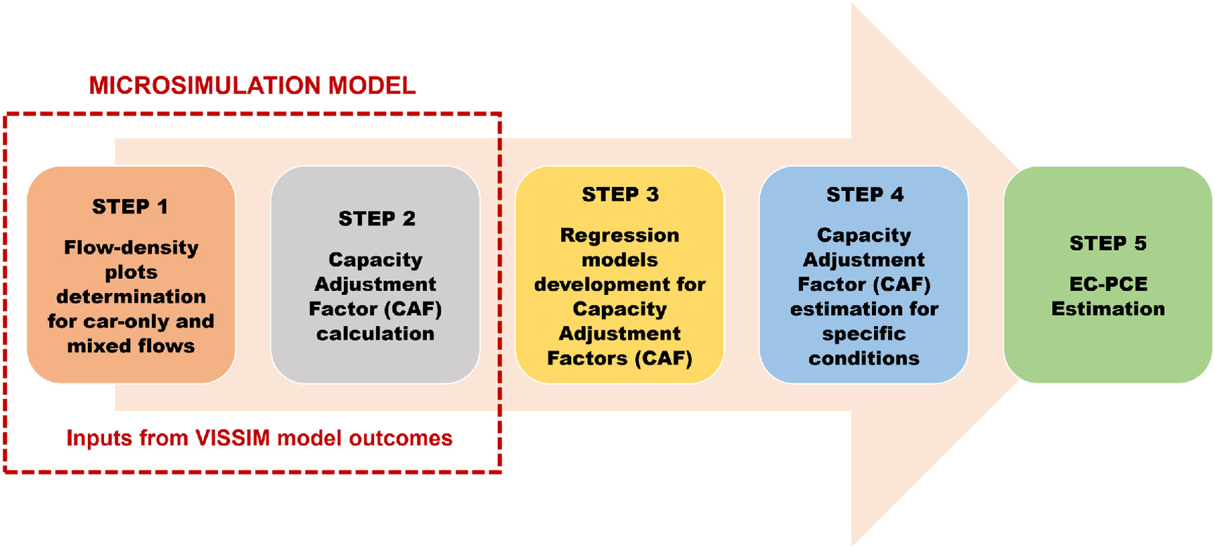
The HCM-6 EC-PCE methodology is composed of five main steps, as shown in Fig. 1. In Step 1, the simulated capacities for both passenger car–only flow and mixed flow are obtained for various combinations of grade, grade length, truck percentage, and vehicle fleet composition. In Step 2, the CAFs for 1,274 scenarios are calculated. A nonlinear regression model is created in Step 3 that can predict the CAF value as a function of the parameters analyzed in Step 1. These calibrated models are used to estimate CAFs in Step 4. In Step 5, the EC-PCEs for specific combinations of truck percentage, grade, and grade distance are estimated based on the CAF estimates. These are the values provided in the HCM-6. A complete description of the HCM-6 EC-PCE methodology, including the key simulation parameters of the VISSIM model, can be found elsewhere (Zhou et al. 2019; Zhou 2018; Dowling et al. 2014b). A brief description that highlights issues critical for modeling the effects of CAV vehicles is given in what follows.
HCM-6 Model Assumptions
It is important to note that the HCM--PCE values are dependent on the VISSIM 4.4 simulation model; to the authors’ knowledge no empirical data were used to calibrate and validate the HCM-6 capacity and EC-PCE values (Dowling et al. 2014a, b; Yang 2013; Zhou 2018). This approach represents a huge advantage from a modeling perspective; it takes significantly less time to model the 1,274 HCM-6 scenarios versus collecting empirical data and developing statistically based models. In addition, it also allows modelers to study new technologies, such as CAV truck platooning. However, there are a number of issues related to the so-called all-simulation approach adopted by the HCM-6 (Hendrickson and Rilett 2017). For example, the VISSIM developers do not guarantee backward compatibility, so there is no guarantee that the current version, VISSIM 20, will result in the same EC-PCE values as shown in the HCM-6. Since the HCM-6 was released in 2016, no less than five updated versions of VISSIM have been released. Owing to its CAV and platoon modeling capabilities, VISSIM 20 was used in this research. Consequently, a considerable amount of effort was spent ensuring the reasonableness of using this version of VISSIM in this research.
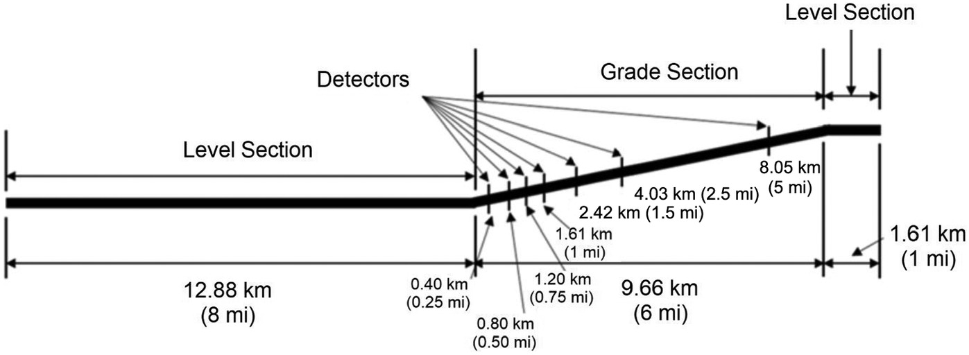
The layout of the HCM-6 test network is depicted in Fig. 2. This test network is a unidirectional freeway segment with three lanes, each (12 ft) wide. The total length of 24.1 km (15 mi) is divided into three sections: (1) an initial level section of 12.9 km (8 mi) to assure that all vehicles may enter in the link regardless of congestion level, (2) an intermediate grade section of 9.7 km () for data collection, and (3) a final level section of 1.6 km (). The intermediate grade section contains seven data collection points (each covering the three lanes). The traffic information obtained at these locations is used as input to the HCM-6 methodology.
The HCM-6 methodology has a large number of assumptions including those related to vehicle speed [e.g., all vehicles travel at the same uniform free-flow speed of ()], vehicle length, weight and power, and driving behavior. A detailed description of the assumptions can be found elsewhere (Dowling et al. 2014a; Zhou 2018). Unless otherwise noted, all assumptions in the original HCM-6 research were followed in this paper.
Note that four factors (e.g., truck percentage, grade, distance, and truck composition type) were examined in the original HCM-6 research. The same factors and scenarios were examined in this paper. In the original research, three truck composition percentages were also explored: (1) single-unit truck (SUT)/tractor trailer (TT), (2) SUT/TT, and (3) SUT/TT. In this paper, only the first scenario was studied because it is the most common on US highways (HCM 2016).
Background Analysis
The most recent version of VISSIM, VISSIM 20, has CAV platoon modeling capabilities. However, the HCM-6 EC-PCE values were calculated using VISSIM 4.4 (Yang 2013). Recent studies have shown that the HCM-6 EC-PCE results can be replicated using VISSIM 9 (Zhou 2018; Zhou et al. 2019). However, assuming that the simulation logic underlying VISSIM releases 4.4 and 9 is the same as VISSIM 20 would be a mistake. It is important to note that the VISSIM developers acknowledge that simulation results can differ among different versions because of changes and updates in the internal logic of the simulator (PTV 2019a). Consequently, the first step was to ensure that the HCM-6 EC-PCE values could be replicated using VISSIM 20. If so, then the results of this CAV analysis in this paper can be compared directly to the HCM-6 results.
The first step was to compare the capacity values obtained from VISSIM 20 and 9 for all scenarios included in the HCM-6. In these experiments, all the simulation parameters were set equal to the HCM-6 values, and both passenger cars and mixed-flow traffic were analyzed. The results showed that the capacity, defined in the HCM-6 as the 95th percentile of the average flow rate, of the passenger car–only condition was 6.54% lower, on average, for the VISSIM 20 results compared to the VISSIM 9 results. A paired -test at a 0.05 level of significance showed that this difference was statistically significant. In contrast to the passenger car–only condition, the difference between VISSIM 20 and 9 for the mixed-traffic condition was only 0.60% on average, and this was not statistically significant at the 0.05 level of significance.
Based on the aforementioned results, it was decided to use VISSIM 20 for the mixed-flow simulations and VISSIM 9 for the passenger car–only flow condition because it was assumed that this would give the best chance for replicating the HCM-6 results. This assumption will be verified subsequently in this paper. The steps for replicating the HCM-6 EC-PCE values are described in what follows.
Step 1: Flow-Density Plots
In Step 1, the flow-density plots of each scenario are created based on output from the VISSIM model. Following HCM-6 protocols, each scenario is simulated using a single run and the same seed number. There are nine volume levels (e.g., 240, 600, 1,200, 1,800, 1,920, 2,040, 2,160, 2,280, ) in every run, and these correspond to volume-to-capacity ratios of 10%–100% based on an assumed theoretical capacity of . Each volume level consists of 1 h of vehicle loading to achieve a steady-state condition, 1 h of steady-state for data collection, and 1 h of vehicle unloading. As a result, the simulation period comprises a total of per scenario (e.g., 3 h per volume level × 9 volume levels). The scenarios are defined by a combination of the following factors:
•
2 flow-rate types (), either passenger car–only or mixed-traffic flow;
•
13 levels of truck percentage () from 2% to 100%;
•
13 levels of grade () from to 6%; and
•
7 levels of grade distance () from 0.40 km (0.25 mi) to 8.05 km ().
In total, there are 91 scenarios for the passenger car–only flow condition (e.g., ) and 1,183 scenarios for the mixed-traffic flow condition (e.g., ). The VISSIM model output consisted of the space mean speed and the flow rate collected at each detector per interval. These outputs are used to compute the hourly flow rate and density, at averages, for each combination using Eqs. (1) and (2), respectively:where = flow rate for flow type at time interval, truck percentage level, truck composition level, grade level, distance level, and simulation flow-rate level based on interval traffic volume recorded by the detector (); interval traffic volume recorded by detector for flow type at time interval, truck percentage level, truck composition level, grade level, distance level, and simulation flow-rate level (); = density for flow type at time interval, truck percentage level, truck composition level, grade level, distance level, and simulation flow-rate level (); interval space mean speed for flow type at time interval, truck percentage level, truck composition level, grade level, distance level, and simulation flow-rate level ().
(1)
(2)
The hourly flow-rate and density values populate the scatter plots for each scenario. There are 1,274 scatter plots in total. Each flow-density scatter plot for a given scenario contains 540 pairs of flow-rate and density values (e.g., levels).
Each scatter plot is used to identify the capacity value for a given scenario. Note that in the HCM-6, capacity is defined as the 95th percentile of the maximum average flow rate for the given scenario (Dowling et al. 2014a, b; Yang 2013). To the authors’ knowledge, this is the first time that the HCM has used an aggregation level other than to calculate a traffic-flow metric. Therefore, care must be taken in comparing the capacity values found in the HCM-6, and by definition in this paper, with other published capacity values that are based on larger aggregation levels. The simulated capacity for each of the 1,274 scenarios is calculated using Eq. (3). Note that if the 540 observations from each scenario were ordered from smallest to largest, the 95th percentile value would be the 513th largest observation:where = capacity for flow type at truck percentage level, truck composition level, grade level, and distance level (); = 95th percentile; and = flow rate for flow type at time interval, truck percentage level, truck composition level, grade level, distance level, and simulation flow-rate level, based on sixty interval traffic volume recorded by detector ().
(3)
To illustrate, Fig. 3 shows a graph of flow rate versus density for the passenger car–only flow, 3% grade, and 1.61 km () distance scenario. It may be seen that the relationship between flow rate and density is linear. Using Eq. (3), the definition of the HCM-6 EC-PCE methodology, the capacity is found to be .
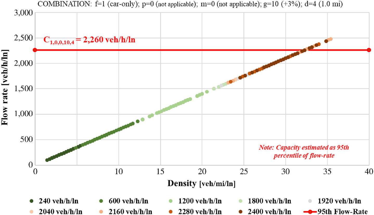
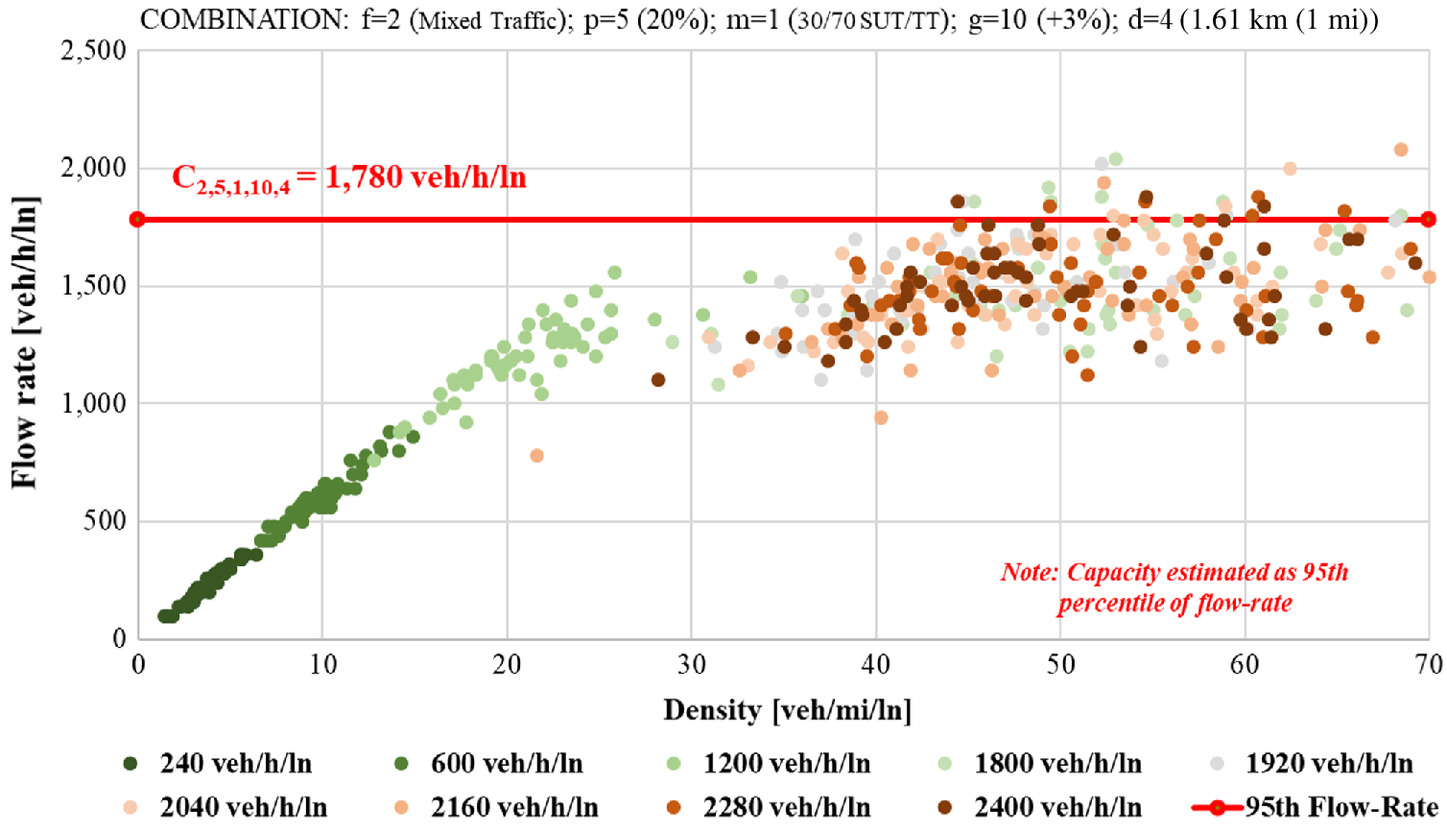
Fig. 4 shows the flow-rate versus density graph for the same conditions as Fig. 3 but for the mixed-traffic flow condition and a 20% truck percentage. It may be seen that at low density, the relationship between flow-rate and density is linear. A breakpoint occurs at approximately 25 veh/mi/ln, and the capacity value is estimated to be .
Step 2: Computation of CAFs from Simulation Output
In this step, the CAFs for each scenario are calculated using the simulation results from Step 1. These are calculated for the mixed-flow and passenger car–only scenarios using Eqs. (4) and (5), respectively. These equations use the capacity of each scenario obtained from the flow-density scatter plots from Step 1:where = capacity adjustment factor for mixed flow at truck percentage level (), with the truck composition level (), the grade level (), and the distance level (); = capacity adjustment factor for auto-only flow at grade level () and distance level (); = capacity for mixed flow at truck percentage level, with truck composition level, grade level, and distance level (); and = capacity for auto-only flow at grade level and distance level ().
(4)
(5)
To illustrate, consider the scenario defined by mixed flow (), 20% truck percentage (), SUT/TT truck composition (), grade (), and 1.61 km () distance (). Note that the passenger car–only and mixed-traffic scatter plots for this situation were shown in Figs. 3 and 4, respectively. Using Eq. (4) the CAF for this situation () is 0.788 (). This calculation is repeated for the other 1,273 scenarios using either Eq. (4) or Eq. (5), as appropriate for the given flow type.
The CAFs for all 1,274 scenarios are shown in Fig. 5. The -axis represents the scenario number. Each specific scenario number is calculated using Eq. (6) and is a function of the truck percentage, grade, and distance. There were 14 truck percentage values (including 0%), and these are shown at the top of Fig. 5. The thinnest line in the background represents the simulated CAFs from this paper and the lower thick line the estimated CAFs obtained in the original HCM-6 research. The blue line will be discussed in Step 4. For a given truck percentage, the CAFs for grade and grade distance are shown in order. The general form is a flat straight line for the negative and zero grade scenarios, followed by decreasing CAF values for the positive grade values:where = scenario number; = ordinal number of truck percentage level ( indicates a 2%–100% truck percentage); = total levels of truck percentage, ; = ordinal number of grade level ( means –6% to 6% grade); = total levels of grade, ; = ordinal number of distance level (level of detector location) ( means (); and = total levels of distance (detector location), .
(6)
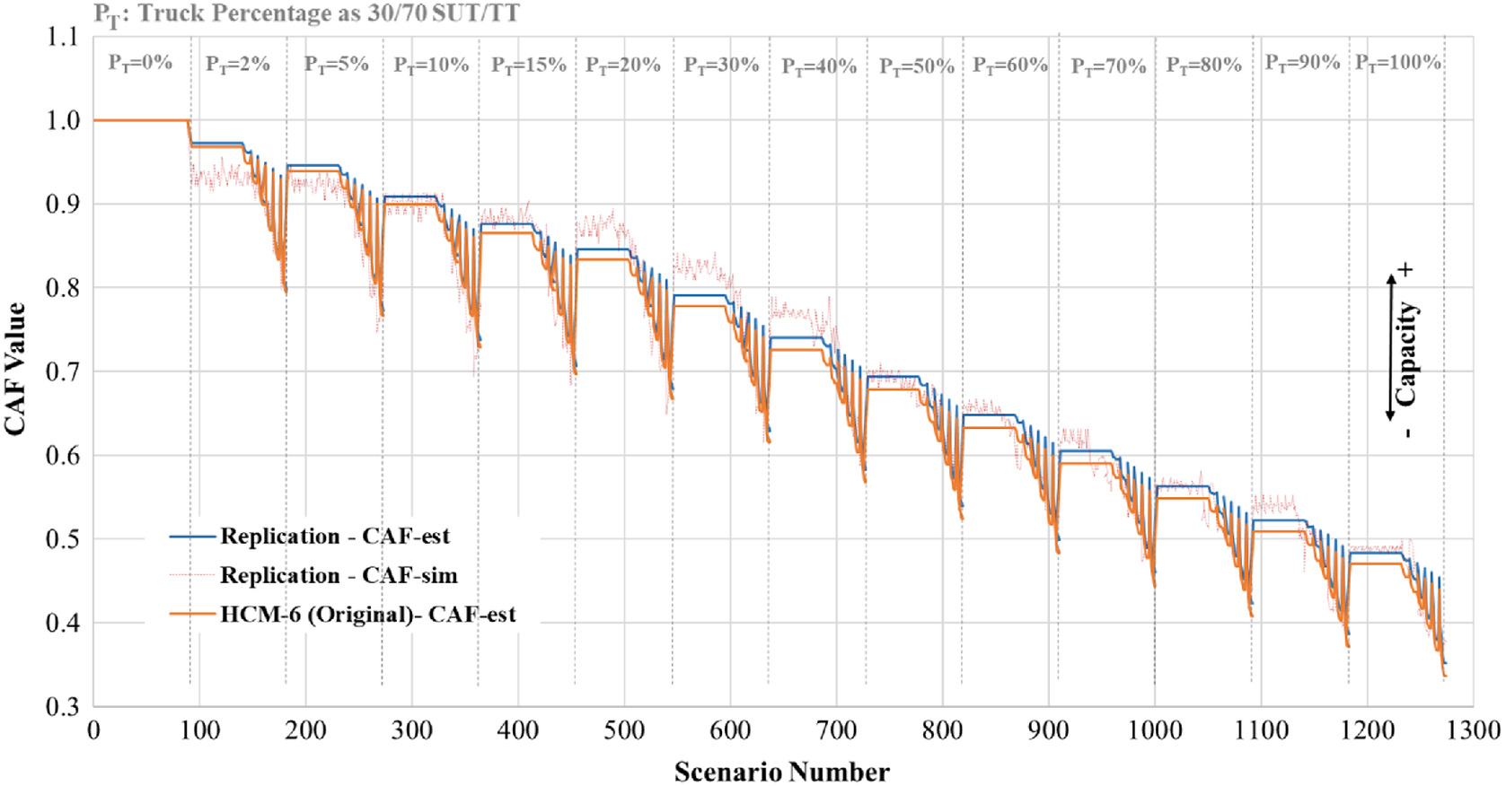
All else being equal, a greater CAF value indicates a higher capacity of the freeway segment. A visual analysis suggests that there is a good match between the estimated CAF values from the two sources. This closeness will be examined statistically in the next section. Note that the CAF values from the HCM-6 are fairly stable while the simulation values tend to have considerable variability. This difference will be explained in the following section.
Step 3: Regression Model Development for Estimated CAFs
Because of the inherent variability of the CAF results from the simulation, the HCM-6 developers chose not to use the simulated CAF values directly. Instead, they calibrated a regression model that related the simulated CAF values to the truck percentage, grade, and distance parameters. The goal was to lessen the variability in the CAF results.
The CAF values from Step 2 are used as input, and statistical regression techniques are used to calibrate the model. The nonlinear regression model used in the HCM-6 are shown in Eqs. (7)–(11) (Dowling et al. 2014b; Zhou et al. 2019; Zhou 2018):where = capacity adjustment factor for mixed flow at truck percentage level, truck composition level, grade level, and distance level; = capacity adjustment factor for auto-only flow at grade level and distance level (this value is assumed to be 1); = capacity adjustment factor for truck percentage effect for mixed flow at truck percentage level and truck composition level; = capacity adjustment factor for grade effect for mixed flow at truck percentage level and truck composition level; = capacity adjustment factor for free-flow speed effect for mixed flow at truck percentage level and truck composition level; = coefficient for capacity adjustment factor for grade effect for mixed flow at truck percentage level and truck composition level; = truck percentage at truck percentage level (between 0 and 1); = threshold of truck percentage for calculating coefficient for capacity adjustment factor related to grade with default value 0.01; = grade at grade level (between and 0.06); = distance of grade at distance level (mi); = free-flow speed for auto-only flow (); , = parameters for capacity adjustment factor for truck percentage effect; , , , , , , , , = parameters for capacity adjustment factor for grade effect; and , , , = parameters for capacity adjustment factor for free-flow speed effect.
(7)
(8)
(9)
(10)
(11)
This paper adopted the same form of the nonlinear model [i.e., Eq. (7)] as was used in the HCM-6. The parameters were estimated using a generalized reduced gradient (GRG) approach. This is a nonlinear optimization method that uses an iterative process to optimize a target value. In this paper, the target goal was to minimize the sum of squared errors between the simulated CAFs from Step 2 and the estimated CAFs from the nonlinear regression model. A detailed description of the method can be found elsewhere (Lasdon et al. 1974). Note that the original research did not mention the optimization technique that was applied to find the best estimates of the model parameters.
Table 3 shows the values of the parameters in the CAF model for the original research and for this paper in Rows 1 and 2, respectively. It may be seen that the estimators between both cases are very similar. It is hypothesized that the small differences found are due to the different versions of the simulator.
Step 4: CAFs Estimation for Specific Conditions
In this step, the CAFs for the mixed flow scenarios () are estimated for the specific conditions listed in the HCM-6. The parameters of interest are truck percentage , grade , and distance . These estimated CAFs are obtained using Eq. (7) based on the calibrated parameters shown in Table 3 (Row 2).
Fig. 6 shows a scatter plot of the estimated CAF value from the original HCM research as a function of the estimated CAF value from this paper. There are a total of 1,274 points or comparisons in this figure. It may be seen that the approach adopted in this paper resulted in a linear relationship with a very high value of 0.99. Fig. 5 shows a direct comparison between the CAF values calculated in this paper (upper thick line) and the CAF values from the HCM-6 (lower thick line). Not surprisingly, the CAF values are generally in agreement. It was concluded that using a VISSIM 9 model for passenger cars and a VISSIM 20 model for mixed traffic allowed for an accurate estimation of the HCM-6 values.
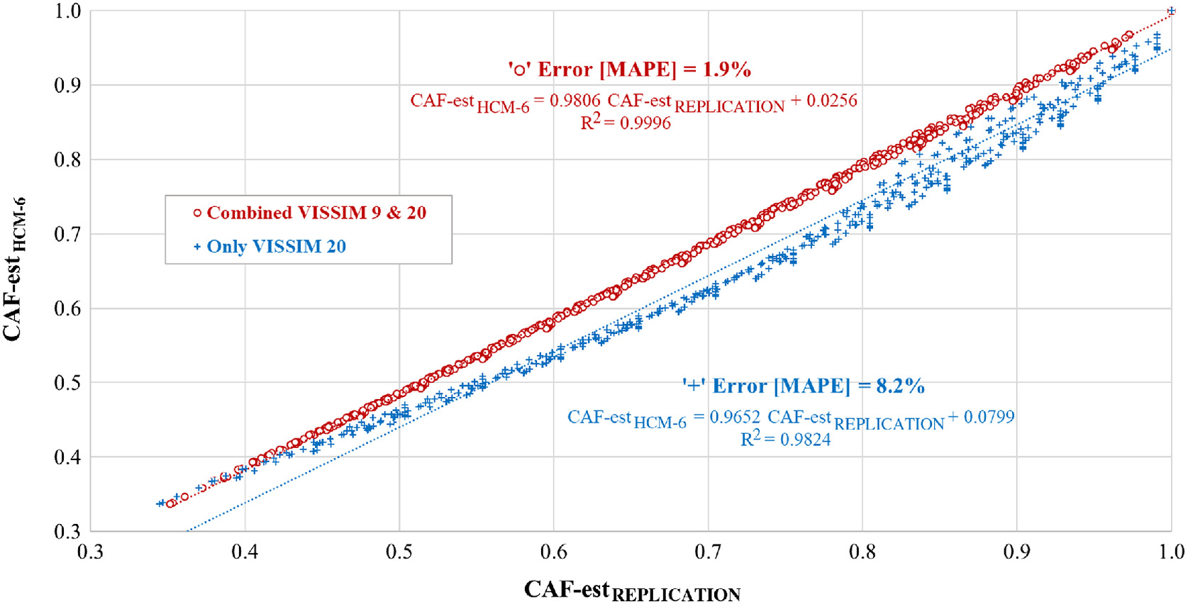
Fig. 6 also shows the relationship between the HCM-6 CAF values and the values obtained if all the simulation data were obtained from VISSIM 20. While the relationship is generally linear, there is considerably more scatter, as evidenced by the mean absolute percentage error (MAPE) value of 8.2%. In addition, the VISSIM 20 CAF results tended to underestimate the CAF values used in the HCM-6. This is why a combination of VISSIM 9 and 20 was used in this paper. Because VISSIM 20 limits lane changing for vehicles traveling at the same speed, it is hypothesized that this adversely affected the passenger car–only simulations (PTV 2019a). With respect to mixed-traffic conditions, this is not as critical as the vehicle characteristics create more lane changing opportunities. This also illustrates a danger in using simulation models for national design guides without adequate controls, such as clearly defining simulation logic and parameters (Hendrickson and Rilett 2017; Rilett 2020).
Step 5: EC-PCE Estimation
In the last step of the methodology, the EC-PCEs () at specific conditions of truck percentage , grade , and distance are calculated using Eq. (12):where = EC-PCE for mixed flow at truck percentage , truck composition , grade , and distance ; = capacity adjustment factor for mixed flow at truck percentage , truck composition , grade , and distance ; and = truck percentage (between 0 and 1).
(12)
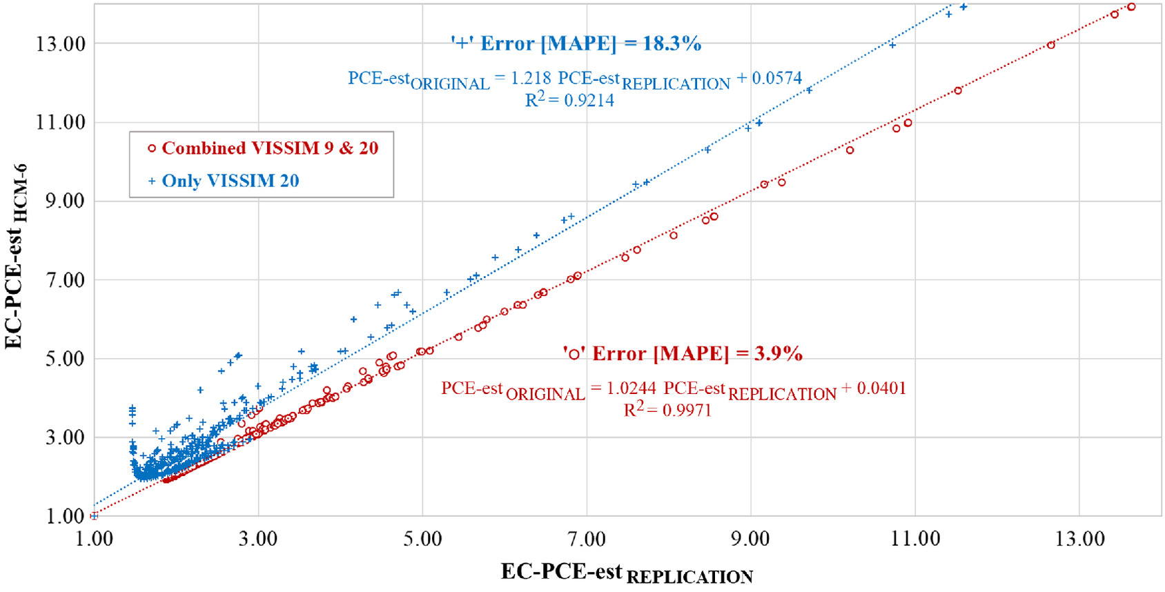
The estimated EC-PCEs as a function of the HCM-6 EC-PCEs are shown in Fig. 7. It may be seen that the relationship is approximately one to one with an value of 0.997 and a MAPE of 3.9%. It was concluded that the simulation approach adopted in this paper can (1) replicate the current HCM-6 values using the HCM-6 assumptions, and (2) be used to model the effect of CAVs on capacity and PCE values using the same HCM-6 approach. Also shown in Fig. 7 is the relationship between the HCM-6 EC-PCE values and the estimated EC-PCE values if only VISSIM 20 were used. While linear, the fit is not nearly as good, as evidenced by the MAPE value of 18.3%.
CAV Modeling Methodology
The HCM-6 methodology, using VISSIM 20 with the parameter sets described previously, was applied to estimate the EC-PCEs when trucks have CAV capabilities. Because the goal of this study was to explore the effect of CAV truck platooning on the capacity of freeway segments, it was assumed that only trucks could operate in CAV mode and that the truck operational characteristics were the same as in the HCM-6. In other words, the only difference between the trucks in the HCM-6 and the trucks in the CAV analysis is that the trucks in the latter scenario could form platoons based on CAV logic.
The VISSIM CAV-related parameter values are based on the CoExist project (Sukennik 2018). The CoExist project is one of the largest research projects to date related to CAV technology. This project was funded by the European Union to prepare the transitional period in which CAVs and conventional vehicles will share roads. The developers of VISSIM, the PTV Group, were responsible for the traffic operation section of the project.
Table 1 shows the parameter set for the CAV vehicles used in this paper. The default driving behavior was AV aggressive (CoExist), which is recommended for CAVs that have full automation (Sukennik 2018). It should be noted that some of the driving behavior parameters were modified to be consistent with the calibrated safety distance parameters (e.g., ) used in the original research. Specifically, the headway time parameter CC1 was set to 0.5 s, instead of the default value of 0.6 s, because this was the value used in the original research. Similarly, the minimum clearance distance was set to , instead of the default value of , because this was the value used in the CoExist project. Note that the analysis in this paper was repeated without making these two minor changes, and the results in this paper were not changed appreciably.
| Model | Parameter | Setting |
|---|---|---|
| Autonomous driving | Enforce absolute braking distance | Unselected |
| Use implicit stochasticity | Unselected | |
| Platooning possible | Selected | |
| Maximum number of vehicles | 7 | |
| Maximum desired speed | () | |
| Maximum distance for catching up to a platoon | ||
| Gap time | 0.5 s | |
| Minimum clearance | ||
| Following | Look ahead | Minimum , maximum |
| Number of interaction objects and vehicles | 10 and 8 | |
| Look-back distance | Minimum , maximum | |
| Behavior during recovery from speed breakdown | ||
| Slow recovery | Unselected | |
| Speed | 60% | |
| Acceleration | 40% | |
| Safety distance | 110% | |
| Distance | ||
| Standstill distance for static obstacles | Unselected | |
| Car following | Wiedemann 99 | |
| CC0 standstill distance | 1.0 m | |
| CC1 gap time | 0.5 s (constant) | |
| CC2 following variation | ||
| CC3 threshold for entering following | ||
| CC4 negative following threshold | ||
| CC5 positive following threshold | 0.10 | |
| CC6 speed dependency of oscillation | 0.0 | |
| CC7 oscillation acceleration | ||
| CC8 standstill acceleration | ||
| CC9 acceleration with | ||
| Following behavior depending on vehicle class | Same as conventional traffic | |
| Lane change | General behavior | Free lane selection |
| Necessary lane change (own and trailing vehicle) | ||
| Maximum deceleration | and | |
| per distance | 100 and | |
| Accepted deceleration | and | |
| Waiting time before diffusion | 60 s | |
| Minimum clearance (front/rear) | ||
| Safety distance reduction factor | 0.75 | |
| Maximum deceleration for cooperative braking | ||
| Overtake reduced speed areas | Unselected | |
| Advanced merging | Selected | |
| Vehicle routing decisions look ahead | Selected | |
| Cooperative lane change | Selected | |
| Maximum speed difference | ||
| Maximum collision time | 10.0 s | |
| Rear correction of lateral position | Unselected | |
| Lateral behavior | Desired position at free flow | Middle of lane |
| Observed adjacent lane(s) | Unselected | |
| Overtake on same lane | Unselected | |
| Exceptions for overtaking vehicles | None |
CAV Base Case
Four major CAV factors were studied. The market penetration rate parameter is defined as the percentage of trucks in a traffic stream with CAV capabilities that would allow CAV platoons to form. The value for the base case was 100%. The lane restriction parameter refers to the number of lanes, starting from the median lane, in which CAV trucks were prohibited from traveling. For the base case, it was assumed that there were no lane restrictions. The platoon truck type factor is related to which truck types, SUT or TT or both, are allowed to join a CAV truck platoon. For the base case, platoons could only form using trucks of the same type. Lastly, the platoon size parameter is defined as the maximum number of trucks that can be part of a given CAV truck platoon. For the base case, this value was set to seven. Sensitivity analyses were used to explore the effect of changing market penetration rate, lane restriction rules, truck platoon vehicles, and truck platoon size on the EC-PCE values.
Modeling the CAV Base Case
The EC-PCE values for the CAV base case scenario were developed using the HCM-6 procedure shown in Fig. 1.
Steps 1 and 2: Simulated CAFs
The 91 passenger car–only scenarios and their associated flow-density plots were developed using VISSIM 9, as described previously. Next, the flow-density plots were developed for the 1,183 CAV scenarios using VISSIM 20. From these plots the HCM-6 capacity, defined as the 95% maximum flow rate using aggregation, was identified. These capacities were then used in Step 2 to calculate the CAF values of the CAV condition for each of the 1,274 combinations.
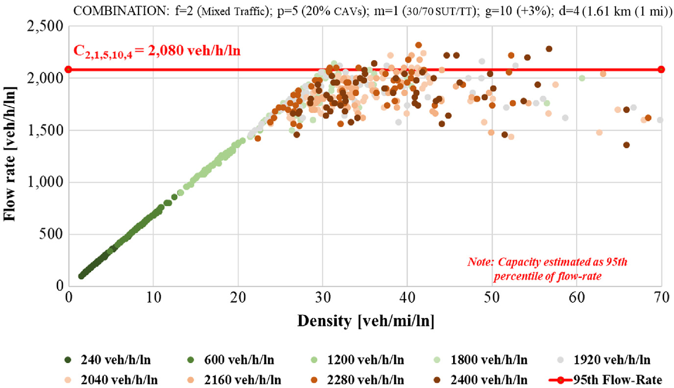
For illustrative purposes, Fig. 8 shows the flow-density curve for the baseline CAV condition for the same conditions as in Fig. 4. It may be seen that the breakpoint occurs at a higher density value (e.g., ). In addition, the CAV capacity (e.g., ) is approximately 10% higher than the equivalent non-CAV capacity (e.g., ). It is hypothesized that the higher capacity occurs due to the deployment of CAV truck platoons in the traffic stream, which vehicles have shorter headways and reduced stochasticity compared to non-CAVs.
Step 3: Nonlinear Model Development
In the original HCM-6 research, a nonlinear regression model was used in Step 3. The form for the HCM-6 analytical model was based on kinematic and resistance equation–related vehicles ascending and descending different grades (Dowling et al. 2014b). A heuristic optimization approach was used to calibrate the model where the goal was to identify the model that minimized the error between the simulated CAFs and the estimated CAFs. The parameters of these equations were optimized using an Excel spreadsheet. The final model consisted of a combined grade and distance effect parameter, a free-flow speed effect parameter, and truck percentage effect parameter (Dowling et al. 2014b; Zhou 2018) as shown in Eqs. (7)–(11).
In this paper, the same model structure was assumed. However, the truck percentage effect () parameter could not be calibrated to an acceptable level. Therefore, it was decided to use four parameters to model this effect. No changes in model format were performed for combined grade and distance effect () and free-flow speed effect (). The statistic that was used to assess model fitting was the standard error of the regression (), as shown in Eq. (13). The advantage of the metric is that it can be applied for both nonlinear and linear models, in contrast to the , which is only valid for linear models (Spiegelman et al. 2011):where = standard error of regression; SSE = sum of squared errors; = number of observations; and = number of parameters in model.
(13)
Seven potential models that attempted to capture the truck percentage effect were analyzed as shown in Table 2. The HCM-6 model, shown as Model 1, is a power function with two parameters. It had an value of 0.0578. Model 4, which is a polynomial model, had an value that was approximately a sixth of the size of Model 1. This model was chosen because it had a low value and fewer parameters compared with other models. Once the final model structure was chosen, the same approach as in the HCM-6 methodology was adopted to find the best estimators for the parameters of the nonlinear regression model.
| No. | Model for truck percentage effect | P | |
|---|---|---|---|
| 1a | 15 | 0.0578 | |
| 2 | 16 | 0.0215 | |
| 3 | 16 | 0.0257 | |
| 4b | 17 | 0.0105 | |
| 5 | 18 | 0.0103 | |
| 6 | 18 | 0.0127 | |
| 7 | 19 | 0.0096 |
Note: = total number of parameters in full nonlinear model; = standard error of regression in CAF units; = truck percentage value; and , and = model parameters relative to truck percentage effect.
a
Original model.
b
Proposed model.
Figs. 9(a and b) show the simulated CAF value versus the estimated CAF values for the original HCM-6 model formulation and the revised model formulation, respectively. It may be seen that the revised model formulation performed much better at predicting the CAF value for a given scenario, as evidenced by the linear relationship shown in Fig. 9(b) and the very high statistic of 0.971.
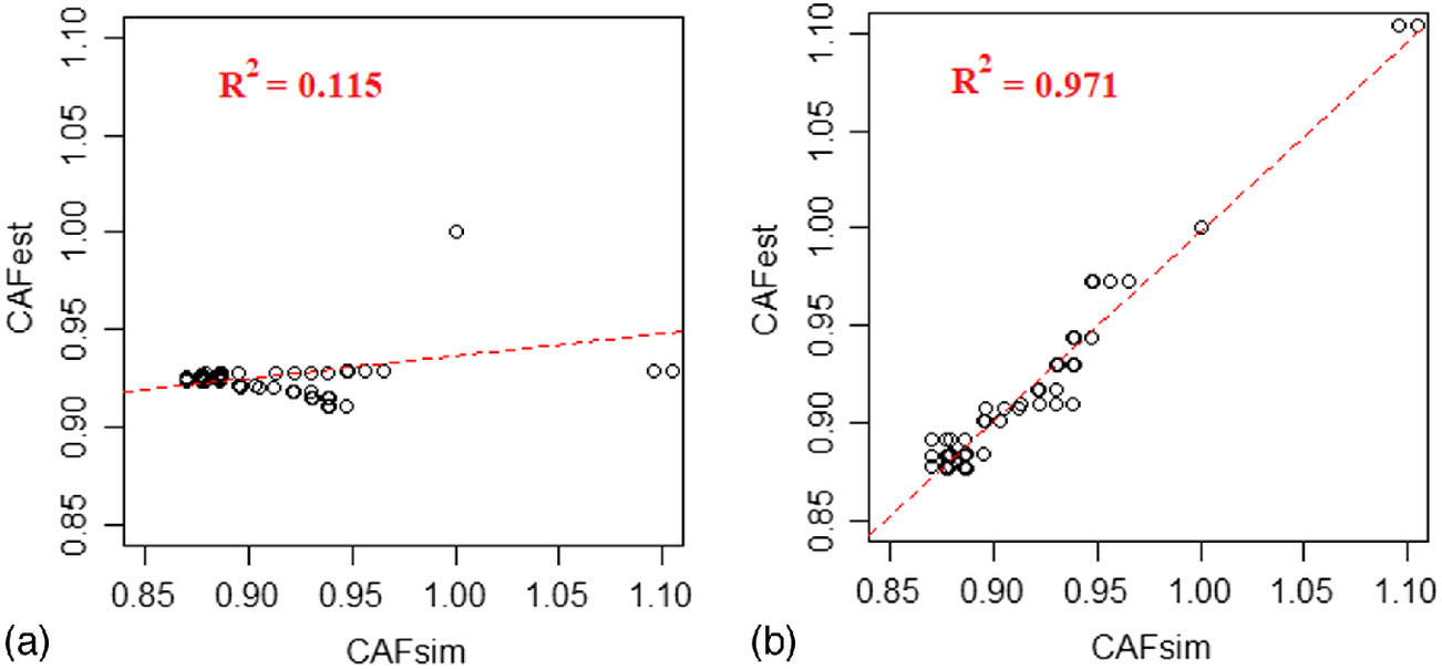
Table 3 shows the model parameters that were used to calculate the estimated CAFs using Eqs. (7)–(11) for each scenario. Row 1 corresponds to the HCM-6 research, Row 2 to the HCM-6 replication described earlier, and Row 3 to the CAV base case described earlier.
| Condition ( SUT/TT) | Nonlinear model parameter | ||||||||||||
|---|---|---|---|---|---|---|---|---|---|---|---|---|---|
| HCM-6 original | 0.53 | 0.72 | — | — | 8.0 | 0.126 | 0.030 | 0.69 | 12.9 | 1.0 | 1.71 | 1.72 | |
| Non-CAV replication | 0.52 | 0.75 | — | — | 8.0 | 0.211 | 0.052 | 1.36 | 5.4 | 1.0 | 1.71 | 1.72 | |
| CAV base case | 0.15 | 0.24 | 7.37 | 8.0 | 0.211 | 0.052 | 1.36 | 5.4 | 1.0 | 1.71 | 1.72 | ||
| Penetration rate | 0.15 | 0.24 | 7.37 | 8.0 | 0.211 | 0.052 | 1.36 | 5.4 | 1.0 | 1.71 | 1.72 | ||
| Penetration rate 75% | 2.41 | 0.30 | 0.30 | 8.0 | 0.211 | 0.052 | 1.36 | 5.4 | 1.0 | 1.71 | 1.72 | ||
| Penetration rate 50% | 0.33 | 0.62 | 10.80 | 8.0 | 0.211 | 0.052 | 1.36 | 5.4 | 1.0 | 1.71 | 1.72 | ||
| Penetration rate 25% | 0.49 | 0.81 | 10.64 | 8.0 | 0.211 | 0.052 | 1.36 | 5.4 | 1.0 | 1.71 | 1.72 | ||
| Two-lane restriction | 0.02 | 0.65 | 1.41 | 8.0 | 0.211 | 0.052 | 1.36 | 5.4 | 1.0 | 1.71 | 1.72 | ||
| One-lane restriction | 0.27 | 5.94 | 0.06 | 8.0 | 0.211 | 0.052 | 1.36 | 5.4 | 1.0 | 1.71 | 1.72 | ||
| Nonlane restrictiona | 0.15 | 0.24 | 7.37 | 8.0 | 0.211 | 0.052 | 1.36 | 5.4 | 1.0 | 1.71 | 1.72 | ||
| Platoon per truck typea | 0.15 | 0.24 | 7.37 | 8.0 | 0.211 | 0.052 | 1.36 | 5.4 | 1.0 | 1.71 | 1.72 | ||
| Platoon any truck type | 0.22 | 0.36 | 1.88 | 8.0 | 0.211 | 0.052 | 1.36 | 5.4 | 1.0 | 1.71 | 1.72 | ||
| Platoon size 9 | 0.39 | 0.69 | 26.19 | 8.0 | 0.211 | 0.052 | 1.36 | 5.4 | 1.0 | 1.71 | 1.72 | ||
| Platoon size 7 | 0.33 | 0.62 | 10.80 | 8.0 | 0.211 | 0.052 | 1.36 | 5.4 | 1.0 | 1.71 | 1.72 | ||
| Platoon size 5 | 0.38 | 0.69 | 6.99 | 8.0 | 0.211 | 0.052 | 1.36 | 5.4 | 1.0 | 1.71 | 1.72 | ||
| Platoon size 3 | 0.39 | 0.70 | 5.89 | 8.0 | 0.211 | 0.052 | 1.36 | 5.4 | 1.0 | 1.71 | 1.72 | ||
Note: Capacity adjustment factor for free-flow speed effect for mixed flow is given by following parameters: ; ; ; and . This factor is equal to zero when the assumed free-flow speed is (), as the case in the original research.
a
Base case scenario.
Step 4: Estimated CAF Results for CAV Base Case
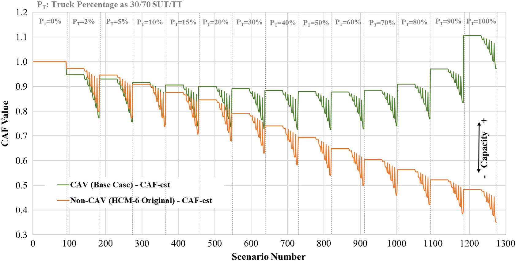
Once the regression models were calibrated in Step 3, the CAFs were then estimated. A comparison of the estimated CAFs for the CAV condition (base case) and the estimated CAFs for the non-CAV condition (e.g., HCM-6 results) are shown in Fig. 10. The increasing line represents the CAV condition and the decreasing line the non-CAV condition. The scenario number (horizontal axis) is given by Eq. (6) and corresponds to a particular combination of truck percentage, grade, and distance that was used to compute the corresponding CAF. For the non-CAV condition, the CAF values decrease as truck percentage increases, and this decrease is at a fairly linear rate. In contrast, for the CAV condition the CAF values increase as the percentage of trucks increase. For truck percentages of less than 10%, the CAF values are similar to the HCM-6. It is hypothesized that this occurs because there are fewer opportunities for truck platoon formation. Interestingly, when trucks are 100% of the vehicle stream, the CAF values are approximately 10.5% higher than the CAF for passenger cars. That is, a traffic stream with 100% CAV will have a higher vehicle flow rate than a traffic stream with 100% passenger cars. Taking as reference the truck percentage interval from 10% to 100% (Scenarios 274–1,274), the CAF values for the CAV condition are, on average, 41.0% higher (ranging from 0.1% to 176.5%) than those of the non-CAV condition.
Step 5: EC-PCE Results for CAV Base Case
Similar to the HCM-6, the EC-PCE values were estimated for 10 levels of truck percentage (i.e., 10%–100% in 10% increments), grade (i.e., 0%, , and ), and distance [i.e., 0.8 km (), 1.61 km (), and 2.42 km ()]. Fig. 11 shows the corresponding EC-PCE values as a function of truck percentage for the three levels of grade and three levels of distance for both the CAV condition (base case) and the HCM-6 values. The solid line represents the CAV EC-PCE values and the dotted line the HCM-6 (e.g., non-CAV) EC-PCE values. The EC-PCE values were calculated using Eq. (12). Note that any specific condition within the explored range of truck percentage, grade, and distance that were considered in the HCM-6 methodology can be computed using the model parameters provided in Table 3. On average, the EC-PCE values for the CAV condition are 34.3% lower than those of the non-CAV condition, indicating that the CAV technology lessens the impact of heavy trucks on traffic operations.
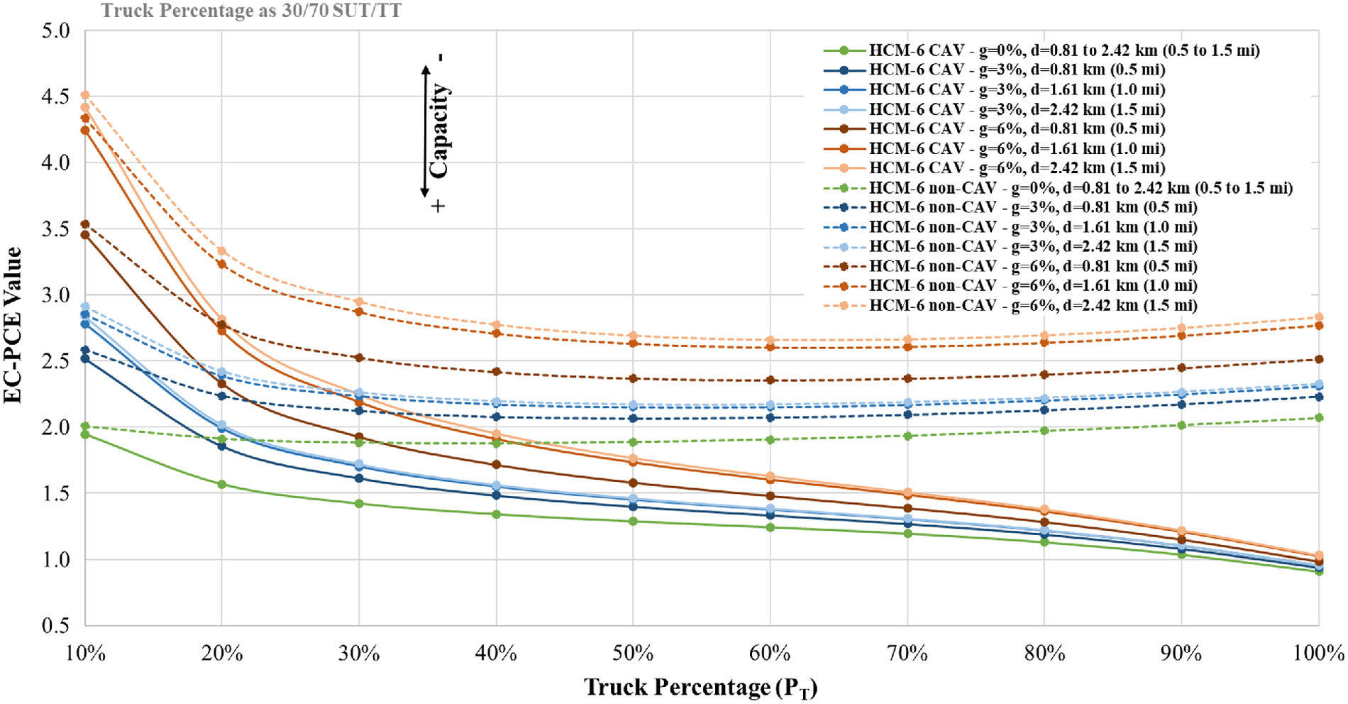
For both the CAV and non-CAV conditions, the maximum EC-PCE values occur at a truck percentage of 10%. These values range from 2.0 to 4.5. In general, as the grade and distance increase, so does the EC-PCE. For higher truck percentages, the EC-PCE values for the non-CAV condition tend to decrease as truck percentages increases until the 30% value is reached. After this point, the EC-PCE values tend to increase at a decreasing rate with truck percentage. In general, the EC-PCE ranges from 2.0 to 4.5 for the non-CAV condition. In contrast, for the CAV condition the EC-PCE decrease at a decreasing rate as percentage of trucks increase. As would be expected from the earlier analysis, as the truck percentage approaches 100% the EC-PCE value approaches 1.
In summary, the CAV technology increases the capacity for a given scenario, all else being equal, and this results in correspondingly lower EC-PCE values. The increase in capacity for a given scenario is a function of the grade, grade length, and percentage trucks in the scenario. It should be noted that this comparison is for trucks equipped with CAV technology. It is hypothesized that if passenger cars also had CAV platoon technology, then the capacity increase shown in Fig. 11 would be even greater. However, it is unclear how the EC-PCE values would change without a detailed simulation study, which is beyond the scope of this paper.
Sensitivity Analysis of CAV Operational Factors
The parameters that were studied in the sensitivity analysis were market penetration rate, lane restriction, platoon truck type, and platoon size as shown in Table 4. Note that the values with an asterisk were considered in the base case scenario described earlier.
| Factor | Scenarios |
|---|---|
| Market penetration rate parameter | 0%, 25%, 50%, 75%, 100%a |
| Lane restriction parameter | No lane restrictiona, one-lane restriction, two-lane restriction |
| Platoon truck type parameter | Restricted (only similar truck types)a, unrestricted (any truck type) |
| Platoon size parameter | 3, 5, 7a, 9 |
a
Base case.
The market penetration rate parameter is defined as the percentage of trucks in traffic demand with CAV capabilities. Four other values, in addition to the base case value of 100%, were analyzed. Three lane restriction parameter values were analyzed, including the base case value of No lane restriction. The one-lane restriction case meant that the leftmost lane could not be used by trucks, while two-lane restriction meant that the two leftmost lanes could not be used by trucks. The platoon truck type parameter included both any truck type, meaning that platoons had no restriction on truck type, and per truck type, indicating that platoons could only consist of similar truck types (e.g., base case). Lastly, four platoon-size parameter values were utilized, and these consisted of 3, 5, 7 (e.g., base case), and 9 for the maximum number of trucks that can be part of a CAV truck platoon.
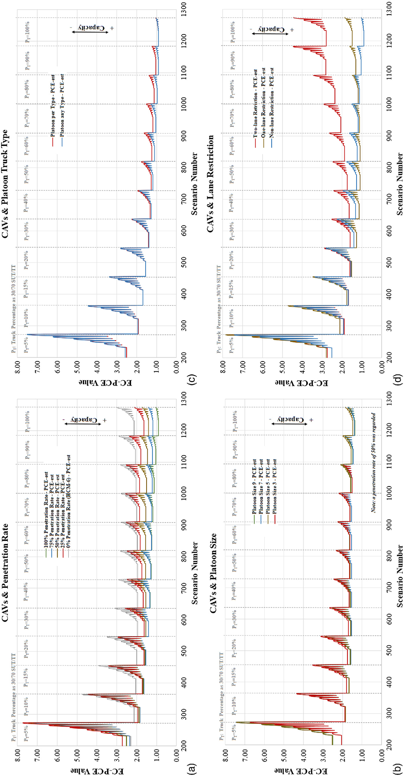
The EC-PCE values as a function of scenario number for each of the four sensitivity analyses are shown in Fig. 12. The scenario number is calculated using Eq. (6) and represents the combination of truck percentage, grade, and distance that was used to compute the corresponding EC-PCE. The EC-PCE values were calculated using the model parameters provided in Table 3, which were obtained following the same HCM-6 methodology used for the CAV base case.
Market Penetration Rate
As may be seen in Fig. 12(a), the EC-PCE values tend to decrease as market penetration rate increases, and this holds true for all truck percentage rates. For truck percentages in a range of 10%–20%, the EC-PCE values for the CAV scenarios are, on average, 15.8% lower compared to the non-CAV condition (0% market penetration rate). For truck percentages in a range of 30%–100%, the EC-PCE values decrease as market penetration rate increases. The decrease for the 25%, 50%, 75%, and 100% market penetration rate is, on average, 12.9%, 25.2%, 37.6%, and 41.3% lower than the corresponding non-CAV scenario, respectively. Interestingly, the market penetration rates of 75% and 100% produce similar EC-PCE values up to the 70% truck percentage level. After this point the 100% market penetration rate scenario performs better with EC-PCE values being, on average, 12.4% lower. In summary, higher market penetration rates tend to produce lower EC-PCE values, indicating that as market penetration rates increase, the impact of trucks on freeway capacity decreases, all else being equal.
Platoon Truck Type: Restricted versus Unrestricted
Fig. 12(b) shows the EC-PCE values as a function of scenario for the truck type parameter. It can be seen that there are only slight differences between the results for the restricted and unrestricted platoon types. For lower truck percentages (e.g., 0%–30%) and the highest truck percentage (e.g., 100%), the EC-PCE values are approximately the same for both scenarios. For truck percentages in the range of 40%–90%, the EC-PCE values for the restricted platoon scenario were, on average, 10.6% greater than the unrestricted platoon scenario. This indicates that limiting platoons to a specific type of truck type could negatively affect freeway capacity compared to the unrestricted implementation. It must be noted that this factor can be affected by the truck composition type, and for this analysis, only one truck composition type was explored ( SUT/TT). It is expected that the differences found would be greater if a different proportion of truck types (e.g., SUT/TT) were considered in the analysis.
Platoon Size
Fig. 12(c) shows the relationship between EC-PCE and platoon size. It can be seen that the maximum platoon size has only a marginal effect on the EC-PCE values. For example, the largest difference between the three-truck platoon value and the nine-truck platoon value is on the order of 4%. It is hypothesized that this result occurred because the interplatoon spacing and the intraplatoon spacing tend to be equivalent near or at capacity conditions. Note that if merging and diverging zones, which are not part of this HCM-6 methodology studied in this paper, were considered, it would be easy to envision platoon size affecting the EC-PCE values. However, the analysis of this aspect was beyond the scope of this paper.
Lane Restriction
Fig. 12(d) shows the EC-PCE values as a function of scenario number for the three lane-restriction scenarios. It may be seen that lane restriction had the greatest effect, in comparison to the other three sensitivity analysis parameters, on EC-PCE values. For truck percentages less than 20%, the three scenarios (e.g., no lane restriction, one-lane restriction, and two-lane restriction), had approximately similar EC-PCE values. However, as truck percentage increased past the 20% level, so too did the EC-PCE values. The two-lane restriction scenario had EC-PCE values that were, on average, 91.8% higher than the base case (e.g., no lane restriction). Conversely, for truck percentages in the range of 20%–80%, the one-lane restriction scenario had EC-PCE values that were, on average 11.5%, lower than the no lane restriction scenario. It was hypothesized that this occurred because there was still sufficient room in the traffic stream for platoons to form and operate. For truck percentages in a range of 80%–100%, the one-lane restriction had on average 33.4% greater EC-PCE values compared to the no lane restriction scenario.
In summary, the effect of lane restriction on capacity is dependent on the truck percentage. The effect of lane restriction is negligible for low truck percentages (20% or below), but it can negatively affect capacity for moderate to high truck percentages (30% or above), particularly if two of the three lanes are restricted.
Conclusions
The objective of this paper was to analyze the effect of CAV trucks on freeway segments using the HCM-6 methodology. In particular, the changes in CAF and EC-PCE values for different operating characteristics were compared. CAV truck platoons are expected to be one of the first technologies deployed on the national highway system. First, the HCM-6 EC-PCEs were replicated using a microsimulation model in VISSIM 20. This VISSIM version was chosen because it can model explicitly CAV trucks and their associated platoons. Note that the original CAF regression model was recalibrated to obtain a better fit between the simulated and estimated results. The impact of CAV technology on freeway capacity was then quantified using the estimated CAF values and the resulting EC-PCE values. Additionally, a sensitivity analysis of four CAV operational factors (e.g., market penetration rate, platoon truck type, platoon size, and lane restriction) was conducted to measure how these parameters affected the results.
Not surprisingly, it was found that CAV truck platoons had the potential to increase capacity on freeway segments, all else being equal. The EC-PCE values for the CAV base case condition, which assumed a 100% CAV market penetration rate for trucks, were approximately 34.3% lower, on average, than those for the non-CAV condition. In other words, CAV trucks have a lower impact on freeway operations than non-CAV trucks. To date, there has been no other analysis of the effect of CAV operations that were based on the HCM-6 methodology, which is the standard analysis and operations guide for US transportation agencies.
Another major finding is that operational factors, which were examined in the sensitivity analysis, tended to have their greatest effect when the truck percentage is greater than 30%. For truck percentage values below this cut-off, the sensitivity analysis scenarios tended to show similar behavior in operating characteristics. It was hypothesized that this occurred because the proportion of CAV trucks was such that the resulting truck platoons, and the associated truck platoon size, were not enough to influence the capacity of the freeway segment. This finding indicates that CAV trucks may have the greatest impact in areas that have higher percentage truck values, such as in the US Midwest.
Note that in the US Midwest, particularly in rural areas, speed limits are higher, the maximum free-flow speeds of trucks and cars are different, and most of the roads are only two lanes in each direction. It is hypothesized that in these areas the positive effect CAV trucks have on capacity will be greater than shown in this paper. According to this paper, conducting analyses for localized conditions is relatively straightforward because the HCM-6 approach is simulation-based. If the conditions described in this paper (e.g., three lanes in each direction, trucks and cars have the same free flow speed) are violated, then it is recommended that the procedure be repeated for local conditions.
It is recommended that the effect of other variables related to driving behavior and operational characteristics, for example, interplatoon spacing, platoon forming logic, weight and power distributions, and acceleration profiles, be studied. These parameters were not studied in this paper owing to space limitations and a lack of empirical data on these topics. This is a potential area of research that would further aid transportation agencies as they begin their transition to CAV operations.
Similarly, the authors believe that using simulations that the current HCM-6 EC-PCE method for freeway segments and multilane highways is based on raises a number of issues that should be addressed in further studies. Because the authors needed to use different versions of the VISSIM microsimulation model than was used in the HCM-6, a recalibration of the nonlinear regression model was required to replicate the results of the original research. It was hypothesized that this was a result of periodic updates and changes in the internal logic of the microsimulation model made by the developer. In addition, the authors would also recommend calibrating the HCM-6 methodology to empirical data. This would also include a deeper assessment of the form and error of the regression models that fit the simulated and estimated data. It is possible that different model structures might provide better results. Finally, it is also recommended that an assessment of the existing simulation assumptions of the current HCM-6 EC-PCE methodology be performed. Interestingly, in the original research, only one simulation run was performed for each scenario combination. This point is crucial because performing a single simulation run drastically increases the noise of the simulation results and could negatively impact the accuracy of the capacity estimates and the associated EC-PCE values.
Data Availability Statement
Some or all data, models, or code that support the findings of this study are available from the corresponding author upon reasonable request.
Acknowledgments
The authors would like to thank the Nebraska Transportation Center for providing the necessary technical tools used in this research. The authors appreciate the contributions of Dr. Jianan Zhou in the replication analysis. The authors would also thank Dr. George List and his colleagues at North Carolina State University for their advice on the 2016 HCM EC-PCE estimation methodology and the background information they provided. It is greatly appreciated. The contents of this paper reflect the views of the authors, who are solely responsible for the facts and the accuracy of the information presented herein and do not necessarily represent any group or agency.
References
AASHTO. 2011. A policy on geometric design of highways and streets. Washington, DC: AASHTO.
ACEA (European Automobile Manufacturers Association). 2017. “What is truck platooning? European automobile manufacturers association.” Accessed December 12, 2019. https://www.acea.be/uploads/publications/Platooning_roadmap.pdf.
Bevly, D., et al. 2017. Heavy truck cooperative adaptive cruise control: Evaluation, testing, and stakeholder engagement for near term deployment: Phase two final report. Washington, DC: USDOT, Federal Highway Administration.
Bujanovic, P., and T. Lochrane. 2018. “Capacity predictions and capacity passenger car equivalents of platooning vehicles on basic segments.” J. Transp. Eng. Part A: Syst. 144 (10): 04018063. https://doi.org/10.1061/JTEPBS.0000188.
Dowling, R., G. List, B. Yang, E. Witzke, and A. Flannery. 2014a. Incorporating truck analysis into the highway capacity manual. Washington, DC: Transportation Research Board.
Dowling, R., G. List, B. Yang, E. Witzke, and A. Flannery. 2014b. Trucks in the freeway analyses of the highway capacity manual. Raleigh, NC: Institute for Transportation Research and Education.
Fitzpatrick, D., G. Cordahi, L. O’Rourke, C. Ross, A. Kumar, and D. Bevly. 2016. Challenges to CV and AV applications in truck freight operations. Washington, DC: Transportation Research Board.
Guanetti, J., Y. Kim, and F. Borrelli. 2018. “Control of connected and automated vehicles: State of the art and future challenges.” Annu. Rev. Control 45 (Jan): 18–40. https://doi.org/10.1016/j.arcontrol.2018.04.011.
Hallmark, S., D. Veneziano, and T. Litteral. 2019. Preparing local agencies for the future of connected and autonomous vehicles. St Paul, MN: Minnesota DOT.
HCM (Highway Capacity Manual). 1965. Highway research board. Washington DC: HCM.
HCM (Highway Capacity Manual). 2016. Transportation research board. Washington DC: HCM.
Hendrickson, C., and L. Rilett. 2017. “Traffic simulation and transportation engineering.” J. Transp. Eng., Part A: Syst. 143 (12): 01817002. https://doi.org/10.1061/JTEPBS.0000091.
Janssen, R., H. Zwijnenberg, I. Blankers, and J. Kruijff. 2015. Truck platooning driving the future of transportation. Hague, Netherlands: Netherlands Organization for Applied Scientific Research.
Kang, S., H. Ozer, and I. L. Al-Qadi. 2019. Benefit cost analysis (BCA) of autonomous and connected truck (ACT) technology and platooning. Reston, VA: ASCE.
Kittelson & Associates. 2019. “HCM CAV CAFs: Capacity adjustment factors for connected and autonomous vehicles in the highway capacity manual.” In Proc., Presentation at the 17th National Transportation Planning Applications Conf. Salem, OR: Oregon Dept. of Transportation.
Konstantinopoulou, L., A. Coda, and F. Schmidt. 2019. “ENSEMBLE: Enabling safe multi-brand truck platooning for Europe.” In Proc., Presentation at the Automated Vehicles Symp., 15–18. Brussel, Belgium: European Commission.
Lasdon, L. S., R. L. Fox, and M. W. Ratner. 1974. “Nonlinear optimization using the generalized reduced gradient method: Revue française d’automatique, informatique, recherche opérationnelle.” Recherche opérationnelle 8 (3): 73–103.
Li, S. E., Y. Zheng, K. Li, L. Wang, and H. Zhang. 2017. “Platoon control of connected vehicles from a networked control perspective: Literature review, component modeling, and controller synthesis.” In IEEE transactions on vehicular technology. Piscataway, NJ: IEEE.
Mahdavian, A., A. Shojaei, and A. Oloufa. 2019. “Assessing the long-and mid-term effects of connected and automated vehicles on highways’ traffic flow and capacity.” In Proc., Int. Conf. on Sustainable Infrastructure, 263. Reston, VA: ASCE. https://doi.org/10.1061/9780784482650.027.
Makridis, M., K. Mattas, B. Ciuffo, M. A. Raposo, T. Toledo, and C. Thiel. 2018. “Connected and automated vehicles on a freeway scenario. Effect on traffic congestion and network capacity.” In Proc., 7th Transport Research Arena TRA. Vienna, Austria: Transport Research Arena.
McHale, G. 2019. “FHWA level 1 truck platooning research program.” In Proc., Presentation at the Automated Vehicles Symp., 15–18. Washington, DC: USDOT, Federal Highway Administration.
PTV (Planung Transport Verkehr). 2019a. PTV VISSIM & VISWALK 2020: Release notes (last modified: 2019-10-09). Karlsruhe, Germany: PTV AG.
PTV (Planung Transport Verkehr). 2019b. VISSIM 20 user manual. Karlsruhe, Germany: PTV AG.
Rilett, L. R. 2020. “Using simulation to estimate and forecast transportation metrics: Lessons learned.” In Proc., CIGOS 2019, Innovation for Sustainable Infrastructure, 23–33. New York: Springer.
Rossen, V. G. 2018. “Autonomous and cooperative vehicles and highway capacity.” Accessed September 28, 2019. https://essay.utwente.nl/76615/.
Shi, L., and P. Prevedouros. 2016. “Autonomous and connected cars: HCM estimates for freeways with various market penetration rates.” Transp. Res. Procedia 15 (Jun): 389–402. https://doi.org/10.1016/j.trpro.2016.06.033.
Spiegelman, C., E. S. Park, and L. R. Rilett. 2011. Transportation statistics and microsimulation. Boca Raton, FL: CRC Press.
Stanek, D. 2019. A procedure to estimate the effect of autonomous vehicles on freeway capacity. Washington, DC: Transportation Research Board.
Sukennik, P. 2018. Micro-simulation guide for automated vehicles. Karlsruhe, Germany: PTV Group.
TTC (Toyota Tsusho Corporation). 2019. “Truck platooning project in Japan.” In Proc., Presentation at the Automated Vehicles Symp., 15–18. Tokyo: Ministry of Economy, Trade and Industry.
Urbanik, T., A. Tanaka, B. Lozner, E. Lindstrom, K. Lee, S. Quayle, and S. Sunkari. 2015. Signal timing manual. Washington, DC: Transportation Research Board.
Yang, B. 2013. “On the HCM’s treatment of trucks on freeways.” Master thesis, Dept. of Civil Engineering, North Carolina State Univ.
Zhou, J. 2018. “Effects of moving bottlenecks on traffic operations on four-lane level freeway segments.” Doctoral dissertation, Dept. of Civil and Environmental Engineering, Univ. of Nebraska-Lincoln.
Zhou, J., L. Rilett, and E. Jones. 2019. Estimating passenger car equivalent using the HCM-6 PCE methodology on four-lane level freeway segments in western US. Washington, DC: Transportation Research Record.
Information & Authors
Information
Published In
Journal of Transportation Engineering, Part A: Systems
Volume 147 • Issue 2 • February 2021
Copyright
This work is made available under the terms of the Creative Commons Attribution 4.0 International license, https://creativecommons.org/licenses/by/4.0/.
History
Received: May 9, 2020
Accepted: Oct 2, 2020
Published online: Dec 4, 2020
Published in print: Feb 1, 2021
Discussion open until: May 4, 2021
Authors
Metrics & Citations
Metrics
Citations
Download citation
If you have the appropriate software installed, you can download article citation data to the citation manager of your choice. Simply select your manager software from the list below and click Download.