Abstract
The latest edition of the Highway Capacity Manual (HCM-6) includes, for the first time, a methodology for estimating and predicting the average travel time distribution (TTD) of urban streets. Travel time reliability (TTR) metrics can then be estimated from the TTD. The HCM-6 explicitly considers five key sources of travel time variability. A literature search showed no evidence that the HCM-6 TTR model has ever been calibrated with empirical travel time data. More importantly, previous research showed that the HCM-6 underestimated the empirical TTD variability by 70% on a testbed in Lincoln, Nebraska. In other words, the HCM-6 TTR metrics reflected a more reliable roadway than would be supported by field measurements. This paper proposes a methodology for calibrating the HCM-6 TTR model so that it better estimates the empirical TTD. This calibration approach was used on an arterial roadway in Lincoln, Nebraska, and no statistically significant differences were found between the calibrated HCM-6 TTD and the empirical TTD at the 5% significance level.
Background
Traffic congestion can be defined as the “travel time or delay in excess of that normally incurred under light or free-flow travel conditions” (Levinson and Margiotta 2011). The variability or changes in travel time on urban arterial roadways are caused by both recurrent and nonrecurrent congestion. Recurrent congestion occurs each day during the same time period (e.g., weekday peak periods) and at the same location on roadways. Nonrecurrent congestion is the result of unplanned or random events, such as inclement weather and traffic incidents.
Road users are usually familiar with recurrent congestion and understand how travel time varies with time of day. However, nonrecurrent congestion, by definition, is unpredictable and causes the most frustration to road users (Tan et al. 2015). Unfortunately, more than half of the causes of traffic congestion are from nonrecurrent sources (Cambridge Systematics 2005). Therefore, understanding how to accurately estimate and predict the variability in congestion is very important in roadway performance analysis.
Historically, measures of central tendency (e.g., mean) are often used to analyze roadway performance. For example, the first five editions of the Highway Capacity Manual express roadway performance as a quantitative stratification of a given performance metric, such as average travel time or density, that represents the quality of roadway service. This is known as the level of service (LOS) (HCM 2010). The LOS is intended to simplify the communication of quantitative performance metrics related to measures of central tendency such as average density or average delay, for example (Roess and Prassas 2014). Logistics companies and commuters are, however, interested not only in the measures of central tendency but also in the measures of dispersion (e.g., variance) because both affect their arrival/travel times (Figliozzi et al. 2011). Consequently, travel time reliability (TTR) metrics, which combine components in measures of central tendency and measures of dispersion, have attracted considerable research interest over the past decade (Taylor 2013).
Reliability has many different definitions in the literature. For example, the Strategic Highway Research Project 2 Report L04 (Mahmassani et al. 2014) described reliability as “the lack of variability of travel times.” Van Lint et al. (2008) used statistical derivations that are based on the skewness of a travel time distribution (TTD) to represent TTR. Dowling et al. (2009) used the standard deviation of a TTD as a proxy for several reliability metrics. Not surprisingly, most studies use the measures of central tendency and measures of dispersion of the TTD for TTR metrics (Arezoumandi and Bham 2011) but not the actual TTD. This paper will focus on the actual TTD. A comprehensive review of the different TTR metrics can be found in Pu (2011).
The US Federal Highway Administration (FHWA) has identified TTR as a key road mobility performance indicator (FHWA and USDOT 2012, 2015). The latest edition of the Highway Capacity Manual (HCM-6) included, for the first time, a methodology for estimating and predicting the TTR on urban arterials (HCM 2016). The HCM-6 states that “travel time reliability reflects the distribution of trip travel time over an extended period. The distribution arises from the occurrence of several factors that influence travel time (e.g., weather events, incidents, work zone presence).” Specifically, the HCM-6 TTR methodology estimates and forecasts the TTD of average travel times by explicitly considering the effect of inclement weather, traffic incidents, demand variations, work zones, and special events (e.g., festivals and game days). TTR metrics such as the travel time index and planning time index can then be determined from the estimated TTD. For example, the planning time index, which is the ratio of the 95th-percentile travel time to the free-flow travel time, compares near-worst-case travel time to free-flow travel time conditions (FHWA Office of Operations and US DOT 2017).
The HCM-6 uses as input (1) supply data (e.g., roadway geometric features), (2) single-day observed traffic demand volume, and (3) historical data on random events, including weather, traffic incidents, and demand variations. The output is an estimated TTD over a user-defined time period.
The literature shows that the HCM-6 approach was validated using the CORSIM simulation model (Zegeer et al. 2014). Critically, there is no documentation that the HCM-6 TTR model was validated or calibrated using empirical travel time data. This was confirmed to the authors during the January 2019 standing committee meeting of the Transportation Research Board’s Highway Capacity and Quality of Services Committee. In addition, it has been shown by Tufuor and Rilett (2020) that the TTD estimated by HCM-6 was statistically different from the empirical TTD on a (1.16-mi) testbed in Lincoln, Nebraska. In particular, the HCM-6 TTR model underestimated the travel time standard deviation by approximately 67%. In other words, the HCM-6 TTR metrics indicated that the testbed was more reliable than field measurements would indicate. Similar results were also shown on a (0.5-mi) testbed in Lincoln, Nebraska (Tufuor and Rilett 2019).
It was found in the analysis that the demand component in the HCM-6 TTR methodology contributed approximately 82% of the estimated error (Tufuor and Rilett 2020). The authors recommended that the first step to improving the HCM-6 TTD estimations is to calibrate the model to local conditions and that the focus of the Lincoln network calibration should be on the HCM demand estimator. Consequently, this paper will use the same testbed and focus on the demand component. The proposed calibration methodology, however, is general and can be used to calibrate the HCM-6 TTR model for all sources of variability, including weather, demand, incident, work zones, and special events.
The remainder of this paper is organized as follows. The next section gives a brief description of the HCM-6 TTR methodology. This is followed by a discussion on the deterministic and stochastic components of the HCM-6 TTR model. A procedure to calibrate the HCM-6 TTR model is then proposed and discussed. Subsequently, the proposed methodology is verified using a case study with real-world data. Lastly, the results are interpreted, and relevant concluding remarks are provided.
HCM-6 TTR Methodology
The following terms are useful in understanding the HCM-6 TTR methodology:
1.
Reliability reporting period (): This is the number of days over which TTR is to be estimated (HCM 2016). The HCM-6 recommends using a 6-month to 1-year reporting period. Note that the user may specify the type of days to be analyzed (e.g., weekdays).
2.
Study period (): This is the time period within a given day () that will be analyzed for each day in the reliability reporting period (). Note that HCM-6 recommends that be a minimum of and a maximum of .
3.
Analysis period (): This is the time interval that is evaluated for each study period. Note that HCM-6 allows for either a 15- or interval.
4.
Number of time periods, of duration , examined in each day (): This parameter is calculated using Eq. (1). Note that must be an integer so that must be evenly divisible by :
(1)
In this paper, the () testbed in Lincoln, Nebraska, that was used in previous studies (Tufuor and Rilett 2020) will be used to illustrate the HCM-6 TTR methodology and the calibration process. The testbed reliability reporting period () is equal to all 261 weekdays in 2016, the analysis period () is , and the study period () is between 4:30 and 5:30 p.m. (PM peak). From Eq. (1), the number of time periods studied in each day () is 4 (e.g., ). From Eq. (2), the number of scenarios () is 1,044.
Fig. 1 shows an overview of the HCM-6 TTR methodology for estimating and predicting TTD and the associated TTR metrics. A full description of the HCM-6 TTR methodology is provided elsewhere (Zegeer et al. 2014; HCM 2016).
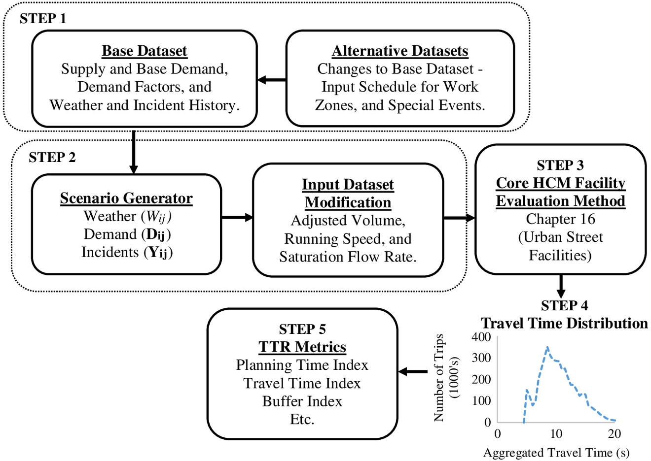
As may be seen from Fig. 1, the HCM-6 TTR methodology has five main steps. In Step 1, data from five key sources that can affect travel time variability (e.g., weather, demand, incident, work zone, and special events) are input. The base data set describes the conditions of the urban arterial where no rain/snow, crashes, work zones, and special events occur. The alternative data sets are used to describe work zone or special-event testbed conditions.
In Step 2, the traffic and weather conditions for each of the scenarios () are created. Adjustments are made to traffic demand volumes, saturation flow rates, and speeds of the base or alternative data set according to the conditions (e.g., weather, demand, and incidents) that occur during a given scenario. These adjustments are based on a Monte Carlo simulation procedure that is based on three random seed numbers, one each for weather, demand, and incident, that are input in Step 1. The scenario-generation process in Step 2 of Fig. 1 will be discussed in subsequent sections.
In Step 3, the HCM Core Facility Evaluation, which is described in Chap. 16 of the HCM-6, is used to estimate the average travel time for each scenario . The estimated average travel times are compiled to form the TTD as shown in Step 4 in Fig. 1. The TTD is then used to estimate the TTR metrics. Some commonly applied TTR metrics are shown in Step 5 of Fig. 1.
The following section provides a brief description of how the weather, volume, incident, work zone, and special events parameter values for each scenario are obtained in the scenario-generation process in Step 2 of Fig. 1. A full description of this scenario-generation procedure is provided elsewhere (Zegeer et al. 2014).
There is a deterministic component and a stochastic component to the scenario-generation process. The active work zone or special event parameters for each scenario are deterministic. The work zone or special event schedule provided in Step 1b of Fig. 1 is used as input in the deterministic process.
The HCM-6 TTR methodology models traffic demand volume variation using three demand factors: an hour-of-day factor (), a day-of-week factor (), and a month-of-year factor (). The traffic demand volume of each intersection/access point movement in each scenario is estimated by a two-step process. First, the demand modification factor (DMF) for each scenario is estimated using Eq. (3):where = demand modification factor for scenario ; = hour-of-day demand factor for scenario ; = day-of-week demand factor for scenario ; = month-of-year demand factor for scenario ; = hour-of-day demand factor for base volume in Step 1 of Fig. 1; = day-of-week demand factor for base volume in Step 1 of Fig. 1; and = month-of-year demand factor for base volume in Step 1 of Fig. 1.
(3)
The second step is to estimate the traffic demand volume of each movement in each scenario using Eq. (4). This is the product of the DMF () from Eq. (3) and the base traffic demand volume that was input in Step 1 of Fig. 1:where = traffic demand vector containing all volumes on intersections and segments in scenario ; and = traffic demand vector containing all volumes on intersections and segments in Step 1 of Fig. 1.
(4)
The uncalibrated hour-of-day, day-of-week, and month-of-year demand factors and the distribution of the DMFs for the testbed conditions are shown in Fig. 2. It may be seen from Fig. 2(a) that there are five day-of-week (e.g., Monday–Friday) and 12 month-of-year demand factors (e.g., January–December). Because the analysis period was from 4:30 to 5:30 p.m., two hour-of-day demand factors (e.g., 4:00–5:00 p.m. and 5:00–6:00 p.m.) were applied. Specifically, the two periods from 4:30 to 5:00 p.m. used the HCM 4:00–5:00 p.m. demand factor, and the two time periods from 5:00 to 5:30 p.m. used the HCM 5:00–6:00 p.m. demand factor. In total, there were 120 unique combinations of demand factors for the testbed example for 2016.
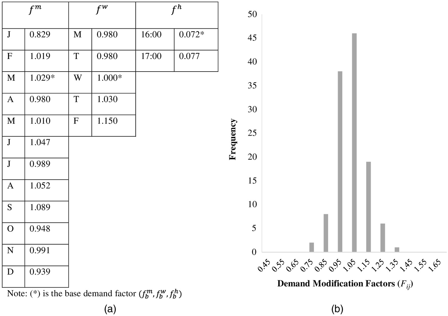
It may be seen from Fig. 2(b) that the distribution of DMFs has a low variance as evidenced by the fact that the range is small (0.75–1.35) and highly peaked around the mean. In addition, approximately 95% of the data falls between 0.95 and 1.15. The DMFs in Fig. 2(b) will be used to adjust the base traffic demand volumes to obtain the demand volume, , for all scenarios, as shown in Eq. (3). Therefore, the distribution of the demand volumes for each scenario, , will have a similar distribution because it is the product of the input volume vector for the given scenario and the scalar DMF for that scenario, as shown in Eq. (4). In other words, the adjusted traffic demand volumes, , will correspond to 95%–115% of the base traffic demand volume. Note that if the user chooses a analysis period, , then the volumes identified in Step 2 will be deterministic, as described previously. If the user chooses a analysis period, then the volumes for each scenario will be derived from a Monte Carlo simulation, as discussed in what follows.
The stochastic component of the scenario-generation procedure in Step 2a of Fig. 1 is composed of three sequential procedures. First, weather event values, , are calculated for each scenario . Second, if a evaluation period is selected, the traffic demand volumes, , for all scenarios are estimated. Lastly, the weather and demand information is used to predict traffic incident value, , for each scenario . The detailed description of the weather events, demand variations, and traffic incident procedures are provided elsewhere (Zegeer et al. 2014).
In summary, up to seven stochastic variables can be used in the HCM-6 TTR model. These 7 stochastic variables are a function of up to 54 weather, demand, and incident variables that are input in Step 1. The exact number of variables will be a function of the application. For the testbed examined in this paper, there are 30 variables. A Monte Carlo sampling method is used to randomly assign a weather event (e.g., rain, snow, and neither rain nor snow), traffic demand volume (if analysis period is selected), and incident event (e.g., incident or no incident) to each scenario . The underlying sampling probability distributions and their corresponding properties for the seven stochastic variables are shown in Table 1.
| Stochastic component | PDF parameters | |
|---|---|---|
| Weather variables | ||
| Precipitation prediction for a given day | Binomial | , |
| where = number of days with precipitation of 0.0254 cm () or more in month ; and = number of days in month | ||
| Precipitation type | Normal | , |
| where = normal daily mean temperature in month . | ||
| If the randomly selected , then the precipitation type is rain, else it is snow. | ||
| Rain intensity (rainfall rate and total rainfall) | Gamma | Rainfall rate () in day of month (): |
| Total rainfall intensity () on day of month , : | ||
| , | ||
| where = total rainfall for rain event in month , ; and = standard deviation of total rainfall in a month, | ||
| . = min (, 0.65) | ||
| Demand variables | ||
| Turn movement traffic demand volume at each signalized intersection | Gamma | Mean , standard deviation = |
| where | ||
| Traffic demand volume on each driveway access point | Poisson | |
| Normal | ||
| , | ||
| standard deviation = | ||
| Incident variables | ||
| Incident occurrence | Poisson | Mean = |
| where = expected hourly incident frequency for street location under a predicted weather condition (); and = proportion of incidents for street location under a predicted weather condition | ||
| Incident duration | Gamma | Mean = , SD = , |
| where = average incident duration for street location type , weather condition , event type , lane location , and severity (h) | ||
Specifically, every scenario will have a binary variable indicating the status of a weather event (e.g., 0 = no weather event and 1 = weather event). The value of this variable is obtained from a Monte Carlo simulation. If a weather event is modeled as occurring in , then the precipitation type, the amount of precipitation, and the length of time the pavement remains wet after the event are also determined using a Monte Carlo simulation.
Similarly, every predicted incident () in a scenario will have information on the type of incident (crash or noncrash) and the location (segment or intersection) on the subject facility. This is also determined using a Monte Carlo simulation.
If a analysis period is chosen, the volume on all segments and driveways is also estimated using a Monte Carlo simulation where the mean volume is based on the corresponding traffic demand volume. Note that separate Monte Carlo sampling is used for roadway segments and driveways, as shown in Table 1.
Because the underlying stochastic processes are modeled using a Monte Carlo simulation, if the random seed number changes, then the corresponding stochastic parameter values will also change. In particular, the values of , (if a analysis is chosen), and will change, and this will affect the resulting TTD in Step 4 of Fig. 1.
Because of the stochastic nature of the HCM-6 TTR procedure, the HCM-6 developers recommend that the procedure shown in Fig. 1 be repeated times, each with a different random seed number, so that the results are robust and not dependent on a single run (HCM 2016). In this paper, was set to four replications, and the resulting average travel time for each scenario was randomly selected from the corresponding scenario in these four replications to form the final estimated TTD.
By definition, changing the input parameters that influence the seven weather, demand, and incident variables of the stochastic components in the HCM-6 TTR model will change the resulting TTD. Note that for the example problem, there are potentially 30 input parameters (e.g., 4 weather parameters, 7 incident parameters, and 19 demand factor parameters) that will affect the values of the 7 stochastic variables in the HCM-6 TTR model. Therefore, changing these input variables will change the HCM-6 estimated TTD. This is the basis of the calibration methodology proposed in the next section.
Proposed HCM-6 Calibration Methodology
Fig. 3 shows the proposed calibration methodology. It can be seen that the proposed calibration framework is an iterative process that consists of five major steps.
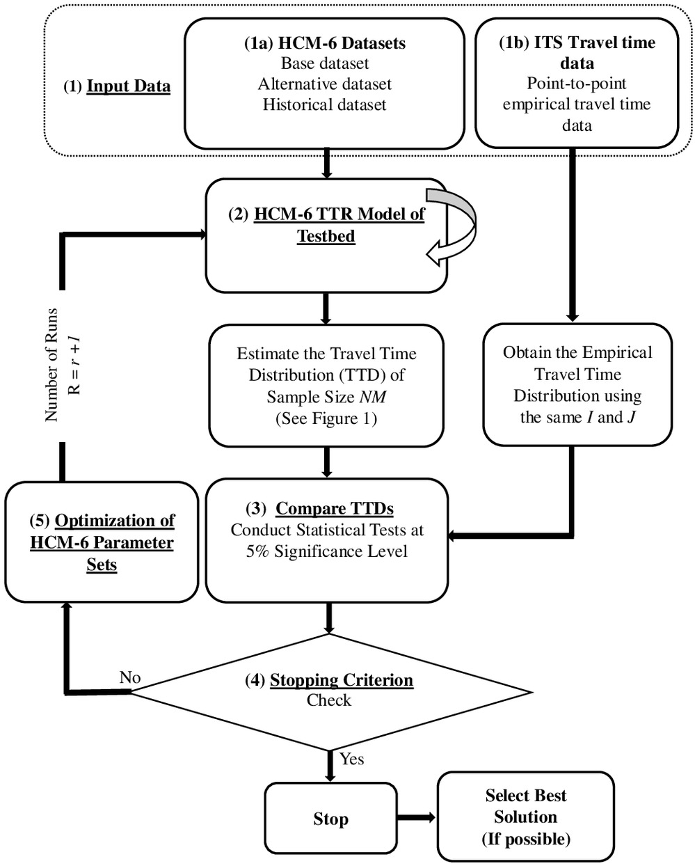
Step 1. Input Data
In this step, two categories of input data are required. The first category, Step 1a in Fig. 3, is the base data set, alternative data set, and historical data set used in the HCM-6 TTR model. In this paper, the testbed weather, volume, and incident input data were obtained from local sources. A discussion of the input values is provided elsewhere (Tufuor and Rilett 2020).
The second category is shown as Step 1b in Fig. 3; it is the observed point-to-point travel time data. Recent advancements in intelligent transportation systems (ITSs), computer technology, and the Internet of things bring with it the potential for collecting more detailed and consistent real-time arterial point-to-point travel time data. Examples of widely used ITSs for data collection include crowdsourcing (e.g., INRIX 2020), connected and automated vehicles (e.g., Datta et al. 2016), and Bluetooth (BT)/wireless fidelity (Wi-Fi)/light fidelity (Li-Fi) detectors (e.g., Cotten et al. 2020).
In this paper, point-to-point ITS travel time data from BT detectors installed on the testbed were utilized. The BT data collection system, its validation, and analysis are discussed elsewhere (Tufuor and Rilett 2018, 2019). The BT data were aggregated, according to the HCM-6 protocol, to obtain average weekday travel times for the analysis period (e.g., 4:30–5:30 p.m.). The data were filtered to eliminate periods that occurred during special events (e.g., public holidays) in 2016. The resulting TTD will form the so-called ground truth, and the goal will be to adjust the TTR model parameters so that the TTD estimated by the HCM-6 TTR model replicates this empirical distribution.
Step 2. HCM-6 TTR Model of Testbed
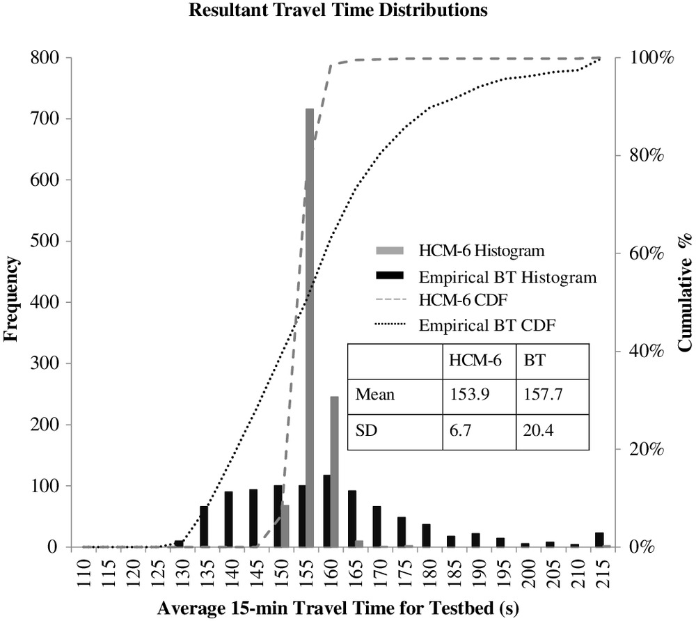
In this step, the current HCM-6 parameter set is used to model the testbed and estimate the TTD.
In the first iteration, the current parameter set corresponds to the uncalibrated parameter values. The BT TTD and the HCM-6 TTD for the first iteration, as well as their corresponding cumulative distribution functions (CDFs), are shown in Fig. 4. It may be seen in Fig. 4 that the empirical BT TTD has considerably more spread compared to the corresponding HCM-6 TTD. It was these differences, described earlier, that motivated this paper.
Step 3. Comparing TTDs
In this step, the TTD estimated by HCM-6 (Step 2) is compared to the empirical BT TTD (from Step 1). Numerous statistical methods exist to test whether two samples from different populations are statistically similar (Spiegelman et al. 2010). Parametric tests, such as Student’s -test and the -test, are popular methods for statistical inference of mean and variance values, respectively. There are two disadvantages to these tests for the purposes of this paper. First, these parametric tests often require a prior assumption of the underlying distribution. This is problematic because often the form of the underlying TTD is unknown. More importantly, these tests do not indicate whether two distributions are statistically similar, and this can be problematic for urban arterial roadway analyses (Kim et al. 2005). Because the goal is to calibrate the HCM-6 TTR model to replicate the empirical TTD, it was critical to use nonparametric or distribution-free tests to statistically determine whether any differences between the distributions were statistically significant. Typical nonparametric tests for comparing two distributions are the Mann-Whitney-Wilcoxon tests and the Kolmogorov-Smirnov (KS) test.
In this paper, the KS test was used to test the hypothesis that the population of the HCM-6-estimated average travel times and the population of the empirical BT average travel times in Fig. 4 have the same distribution. The hypotheses of the KS test is as follows:
Null hypothesis, : .
Alternative hypothesis, : .
Here, is the HCM-6 CDF, and is the empirical BT CDF.
For this test example, a 5% significance level was chosen. Not surprisingly, for the HCM-6 TTD and the empirical BT TTD as shown in Fig. 4, the KS test showed that there were statistically significant differences between the two distributions at a 5% significance level (Tufuor and Rilett 2020).
Step 4. Stopping Criteria
In this step, the stopping criterion (criteria) is (are) checked to determine whether the calibration procedure should continue or not. Because the proposed methodology is an iterative process and there is no guarantee of convergence, at a minimum the analyst needs to set a stopping criterion that will stop the procedure after a maximum number of runs. There is a trade-off between the quality of the results of the iteration and the time spent (Agdas et al. 2018). Traditionally, a set number of iteration loops () is used or suggested for calibration (Spiegelman et al. 2010; Kramer 2017). For this paper, was used and set to 60 because preliminary study showed that 60 iterations (or generations) provided good results for this network. However, if there is no solution after 60 iterations, a new will be set. When the number of iterations equals , the algorithm stops. If not, the algorithm proceeds to Step 5.
Note that the stopping criteria could be a combination of a maximum number of iterations and a specific convergence criterion, such as achieving a successful KS test. The algorithm would stop whenever either criterion was met. In addition, the stopping criteria will be application-specific and may require some experimentation on the part of the user. For example, larger road corridors may need more iterations.
Step 5. Optimize HCM-6 Input Parameter Sets
In this step, a new set of input parameter values is identified. Several optimization algorithms, including the simplex method, genetic algorithm (GA), and simulated annealing, for example, may be used in this step (Kochenderfer and Wheeler 2019). The goal of the algorithm is to select a set of HCM-6 input parameter values for the th run that will result, hopefully, in an estimated TTD that is “better” than the previous () estimated TTD. In this paper, a GA is used to perform this task. A detailed description of the GA process may be found elsewhere (Kramer 2017; Appiah et al. 2011). The GA parameters for this application were selected based on a literature search of previous engineering-related GA applications (e.g., Yao et al. 2012; Yang et al. 2016; Hassanat et al. 2019; Cimorelli et al. 2020). The literature review found that the GA operators, e.g., the crossover rate and mutation rates, ranged from 50% to 90% and 1.0% to 2.5%, respectively. For the testbed, the midrate of the crossover (e.g., 70 %) and mutation (e.g., 1.75%) rates were selected. Twenty parameter sets were analyzed in each generation, and the generation gap was 75%, which was also selected based on experience and previous studies (e.g., Angelova and Pencheva 2011; Roeva and Vassilev 2016). As previously, the best GA values to use will be a function of the application and will, in all likelihood, need to be identified through a combination of prior experience and experimentation.
Since was set to 60, it will be necessary to examine 1,200 parameter sets for the test example. Furthermore, because , the process shown in Fig. 3 was run 4,800 times during the calibration process.
It should be noted that because a statistical test was used in the example problem, once the calibration is complete, there may be one solution, a set of acceptable solutions, or no solution (Kim et al. 2005). If a set of acceptable solutions is found, it will be necessary to develop criteria to select the “best” solution. Intuitively, there are many ways to select the “best” solution. Possible selection criteria include using the lowest error, choosing the parameter set that has the least amount of difference with the HCM-6 default parameter values, and engineering judgment of the “best” representation of local conditions.
Calibration Results
As part of the preliminary analysis, the proposed methodology was used to separately calibrate the TTR model based on three conditions: (1) modifying only weather parameters, (2) modifying only incident parameters, and (3) modifying only demand parameters. It was found that calibrating the weather and the incident parameters did not significantly improve the final TTD. In other words, the KS test failed to obtain any statistically valid solution when the weather and the incident parameters were calibrated. Because there were only 2 incidents and 24 weather events over the reliability reporting period, it was hypothesized that the poor results were due to the relatively small sample size of the weather and incident events on the testbed.
Though the proposed calibration methodology can be used to calibrate all three conditions at the same time, this paper will focus on the results when only the demand parameters were allowed to change during the calibration iterations. For the test example, this meant the 2 hour-of-day demand factors, the 7 day-of-week demand factors, and 12 month-of-year demand factors were allowed to change.
At the end of the calibration, a total of 15 parameter sets, out of the 1,200 parameter sets that were tested, were found to provide statistically significant results. In other words, there were no statistically significant differences between the HCM-6 TTDs derived from these 15 parameter sets and the empirical TTD at the 5% significance level.
Fig. 5 shows the CDFs of the empirical TTD, the HCM-6 TTD (uncalibrated), and the three statistically valid solutions. Note that only 3 of the 15 statistically valid solutions are shown in Fig. 5 for clarity, but all 15 acceptable solutions provided similar CDF curves. It may be seen that the calibrated CDFs and the empirical CDF were very close.
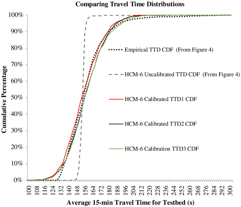
Fig. 6 shows standard boxplots of (1) the empirical BT TTD, (2) the uncalibrated HCM-6 TTD, and (3) the 15 statistically valid solutions. The top, middle, and bottom of each box represent the 75th-percentile, the median, and the 25th-percentile travel times, respectively. The upper and lower boundaries are 1.5 times the interquartile range from the percentile values.
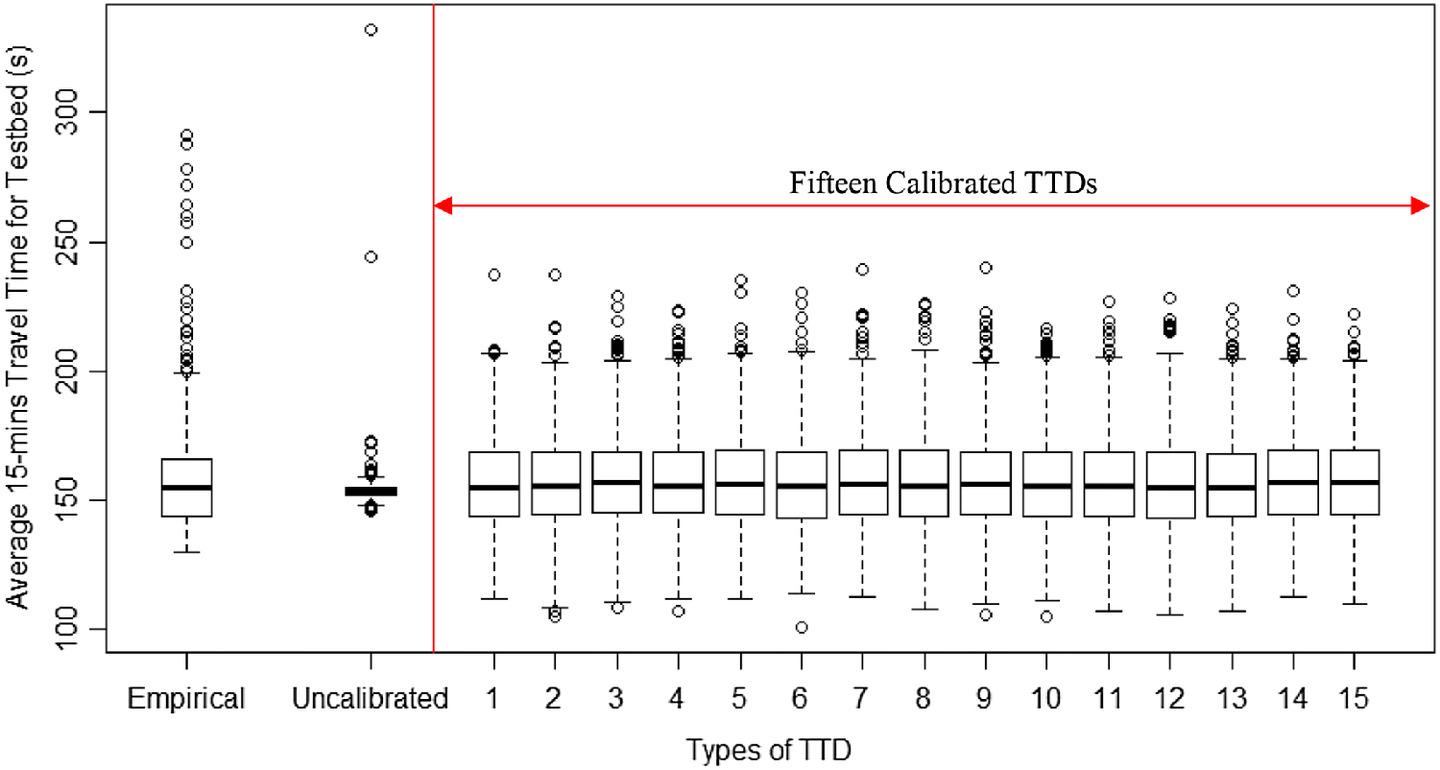
The interquartile range of the uncalibrated HCM-6 TTD is considerably smaller than the empirical TTD. In contrast, the 15 calibrated solutions have an average interquartile range () that is similar to the interquartile range of the empirical TTD (). The only observable difference between the empirical and calibrated TTDs is that the former has more outliers. Similarly, it may be seen that the empirical TTD had a heavier tail when compared to the 15 calibrated solutions. It is plausible that this difference may be the effect of the weather and incident parameters that were held constant in the calibration process. Also, the empirical TTD may reflect other factors that affect the variability in travel time, which the HCM-6 does not consider.
Table 2 shows the descriptive statistics, the statistical test results, and key TTR metrics of the empirical TTD, the uncalibrated HCM-6 TTD, and the three calibrated solutions from Fig. 5. Only three calibrated TTDs are presented due to space limitations. However, it should be noted that the other 12 valid solutions have similar statistics, as presented in Fig. 6.
| Statistic | Empirical | Uncalibrated | Calibration 1 | Calibration 2 | Calibration 3 |
|---|---|---|---|---|---|
| Mean | 157.7 | 153.9 | 156.8 | 157.7 | 156.9 |
| Median | 155.0 | 153.7 | 155.1 | 156.8 | 155.6 |
| Standard deviation | 20.4 | 6.7 | 17.9 | 18.6 | 18.4 |
| 95th percentile | 191.0 | 157.0 | 188.4 | 191.8 | 188.5 |
| Count | 838 | 1,044 | 1,044 | 1,044 | 1,044 |
| Mean absolute error | — | 17.20 | 4.12 | 4.00 | 3.39 |
| Statistic (-value) | |||||
| -test | — | 5.26 () | 1.03 (0.30) | 0.03 (0.97) | 0.93 (0.35) |
| KS test | — | 0.41 () | 0.06 (0.12) | 0.07 (0.05) | 0.06 (0.08) |
| Mann-Whitney-Wilcoxon test | — | 469,930 (0.01) | 432,960 (0.70) | 417,490 (0.09) | 431,780 (0.63) |
| TTR metrics | |||||
| Travel time index | 1.56 | 1.52 | 1.55 | 1.56 | 1.55 |
| Planning time index | 1.89 | 1.55 | 1.87 | 1.90 | 1.87 |
| Level of TTR | 1.10 | 1.01 | 1.10 | 1.10 | 1.11 |
It may also be seen in Table 2 that there were no statistically significant differences between the empirical and calibrated TTDs, their means, and median at the 5% significance level. On average, the difference in mean travel times for the empirical and valid solutions is less than . However, the standard deviations of the calibrated TTDs were, on average, 12% smaller than the standard deviation of the empirical TTD. This may be due to the contribution of the other sources of travel time variability that were not calibrated.
For the testbed, 15 parameter sets provided statistically valid TTDs. A natural question is how to choose among these 15 statistically valid TTDs. One approach is to measure the variations between the two distributions and pick the “best” one. The mean absolute error (MAE) metric estimates the average of the absolute differences between the TTDs and is a direct measurement of the variations between TTDs. It is calculated using Eq. (5):where = frequency of bin of HCM-6 TTD; = frequency of bin of empirical BT TTD; and = number of bins.
(5)
In this paper, for each MAE calculation, the bin width was and the number of bins was 100, which captured travel times from 100 to .
Note that MAE is one of a number of metrics that measure the variations between two distributions. Others include the root-mean-square error (RMSE) and the sum of squared errors (SSE). The MAE was selected in this paper because the error is not weighted, unlike the RMSE, and does not change with the variability of the error magnitudes (Willmott and Matsuura 2005). It should be noted that users can choose any secondary metric or metrics they feel is best for their application.
The MAE values from the testbed are shown in Table 2. The three statistically valid solutions in Table 2 represent the highest MAE (e.g., Calibration 1), the median MAE (e.g., Calibration 2), and the lowest MAE (e.g., Calibration 3). The MAE was for the uncalibrated TTD when compared to the empirical TTD. When the HCM-6 TTR model was calibrated, this value reduced to an average MAE value of for the 15 statistically significant parameter sets. The lowest MAE (Calibrated 3) value was and this was the one recommended for use on this corridor. The MAE values imply that there is a 77% difference in error between the uncalibrated and calibrated TTD. Also, there is an average of 3% error when calibrated compared to a 17% error when the TTD is not calibrated.
Not surprisingly, the three commonly used TTR metrics for the calibrated conditions are similar to the field TTR metrics. It may be seen from Table 2 that the travel time index (TTI), the planning time index (PTI), and the level of travel time reliability (LOTTR) were 3%, 18%, and 8% different than the empirical TTI, PTI, and LOTTR, respectively. In contrast, the TTI, PTI, and LOTTR for the “best” calibrated condition were only 1% different.
The TTI, estimated as the ratio of the mean travel time to the free-flow travel time of the TTD, shows that the testbed is not very congested, as evidenced by the fact that the indexes for the empirical TTD, uncalibrated TTD, and calibrated TTD are all less than 2.5. This implies that the testbed is likely to provide a level of service of “D” or better.
The PTI is the ratio of the 95th-percentile travel time to the free-flow travel time. The PTIs indicate that the testbed is more reliable when uncalibrated than the empirical and calibrated TTDs could show. Similar results are observed for the LOTTR, which is the ratio of the 80th-percentile travel time to the median value. For example, for on-time arrival, a trip maker will have to plan a total of to travel the testbed in the uncalibrated scenario compared to for the empirical case and approximately when calibrated.
Interpretation of Calibrated Demand Parameters
As discussed previously, the calibration process for the example problem focused solely on 19 demand factors. Table 3 shows the HCM-6 uncalibrated and calibrated demand factors and the percentage change between the factors. Also in Table 3 is the calibrated demand factors using only 2 parameters (e.g., mean and variance of the 19 demand factors). The process will be explained in the next section.
| Period | Uncalibrated | “Best” calibrated | Change (% change) | Mean-and-variance calibrated |
|---|---|---|---|---|
| Monday | 0.980 | 0.900 | (8) | 1.147 |
| Tuesday | 0.980 | 0.411 | (58) | 1.141 |
| Wednesday | 1.000 | 0.621 | (38) | 1.110 |
| Thursday | 1.030 | 1.045 | 0.015 (1) | 0.823 |
| Friday | 1.150 | 1.200 | 0.050 (4) | 0.851 |
| January | 0.829 | 0.870 | 0.041 (5) | 1.004 |
| February | 1.019 | 0.930 | (9) | 0.928 |
| March | 1.029 | 1.011 | (2) | 1.051 |
| April | 0.980 | 1.032 | 0.052 (5) | 1.153 |
| May | 1.010 | 1.053 | 0.043 (4) | 0.828 |
| June | 1.047 | 1.068 | 0.019 (2) | 1.003 |
| July | 0.989 | 1.060 | 0.071 (7) | 1.004 |
| August | 1.052 | 1.056 | 0.003 (0) | 1.048 |
| September | 1.089 | 1.020 | (6) | 0.899 |
| October | 0.948 | 1.010 | 0.062 (7) | 0.951 |
| November | 0.991 | 0.980 | (1) | 0.898 |
| December | 0.939 | 0.940 | 0.001 (0) | 0.880 |
| 4:00 p.m. | 0.072 | 0.060 | (17) | 0.051 |
| 5:00 p.m. | 0.077 | 0.080 | 0.003 (4) | 0.099 |
It may be seen in Table 3 that the differences between the uncalibrated and calibrated month-of-year and time-of-day adjustment factors are relatively small. For example, the average absolute percentage difference is 4.8%, and the largest difference is 8.9%. In contrast, the average absolute percentage difference between the uncalibrated and calibrated factors for the day-of-week parameter factors is 22.0%. In addition, the largest difference for the Tuesday factor is 56.9%.
The demand factors for both the calibrated and uncalibrated conditions in Table 3 were used to determine their corresponding DMFs using Eq. (3). Fig. 7 shows the distribution of the DMFs for both the calibrated condition and the uncalibrated condition [from Fig. 2(a)].
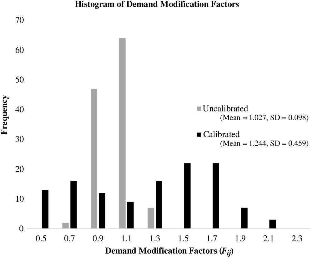
From Fig. 7 it may be seen that the calibrated DMFs have considerably more spread compared to the uncalibrated DMFs. This is evidenced by the fact that the calibrated standard deviation is approximately 78% greater. The calibrated DMF distribution is bimodal. The appropriateness of the bimodality will be discussed subsequently.
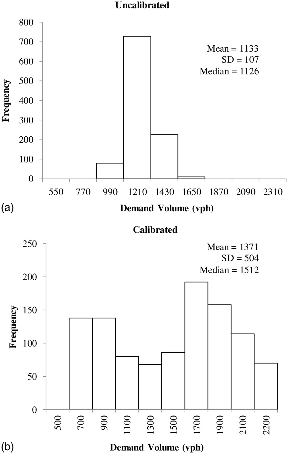
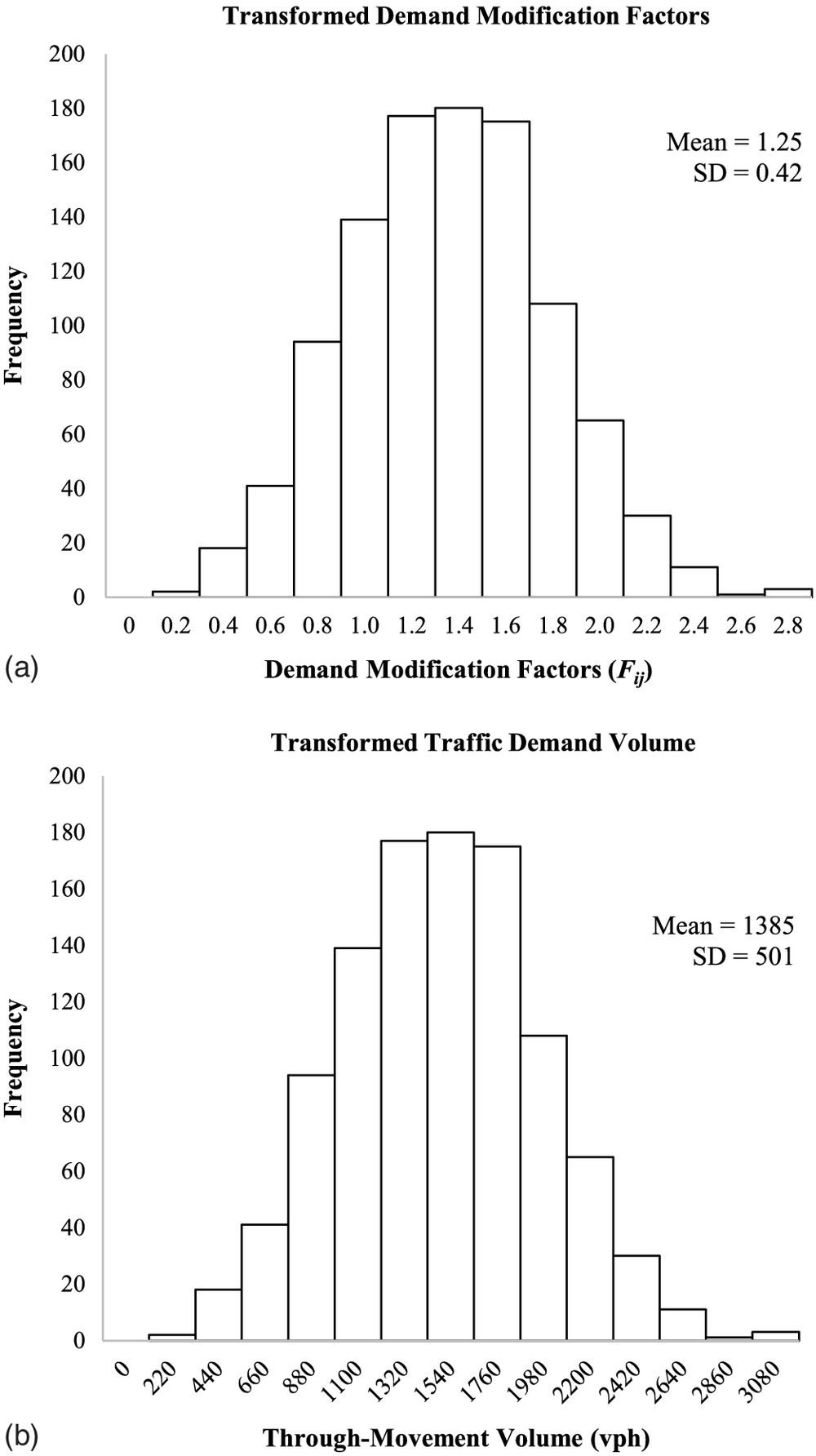
To illustrate how the traffic demand volumes and the demand factors interact, consider the northbound through movement on the first segment of the testbed for a scenario where the base traffic demand volume is 1,100 vehicles per hour (vph). Figs. 8(a and b) respectively show the uncalibrated and calibrated traffic demand volume for only the northbound through movement for the first segment of the testbed. These volumes were obtained using the DMF and the baseline volume in Eq. (3).
It should be noted that similar histograms can be obtained for all intersections and segment movements. The through movement was selected because the HCM-6 TTD is focused on the performance of the major-street through movement (Bonneson 2014).
It may be seen in Fig. 8 that the calibration had two effects on the demand distribution. First, the average through volume increased by 21%, from 1,133 to 1,371 vph. Second, the dispersion of the volumes in the calibrated condition is much greater, as evidenced by the fact that the standard deviation increased by 79%. The increase in both the mean volume and the variability in volume allowed the resulting HCM-6 TTD to match the empirical TTD.
It could be argued that the calibrated demand factors as shown in Table 2 no longer have a “physical” meaning. For example, why would a Tuesday (e.g., 0.411) have 66% less traffic than a Friday (e.g., 1.200), all else being equal? However, it is important to note that the HCM-6 TTD estimation methodology is a mechanistic approach where many solutions (e.g., combination of different values of the demand factors) will give the same answer.
Note that a user may wish for the calibrated DMF distribution to have a “physical” meaning. In this situation, the calibrated bimodal DMF distribution can be transformed into an alternative form that, first, fits the user’s prior knowledge of the demand factor distributions and, second, will still result in a statistically similar TTD when used in the HCM-6 TTR model. A Monte Carlo procedure can be used to randomly simulate and substitute the DMF values with the preferred DMF distribution. The values from the resultant DMF distribution can be used to derive the corresponding hour-of-day, day-of-week, and month-of-year demand factors using simple optimization techniques.
As an example, the user may wish for the DMF distribution to follow a Weibull distribution. The transformed DMF distribution is shown in Fig. 9(a). It may be seen that the distribution is approximately bell-shaped and has mean and variance values that are similar to the calibrated, bimodal DMF distribution. Fig. 9(b) shows the resulting traffic volume for the same through movements as shown in Fig. 8(b). Not surprisingly, this distribution is also bell-shaped. More importantly, it was found that the calibrated DMF distribution in Fig. 7 and the transformed DMF distribution in Fig. 9(a) resulted in similar TTDs when input into the HCM-6 TTR model. These TTDs were compared using the KS test, and there were no statistically significant differences at the 5% significance level. In other words, for this test network it was relatively straightforward to transform the calibrated DMF shown in Fig. 7 to those in Fig. 9(a). Both sets of demand factors will result in statistically valid TTDs. Note that the foregoing procedure was repeated for a lognormal and gamma distribution, and similar results were found.
Two Parameters (Mean and Variance) Calibration
Following from the previous discussions on the transformation of the DMFs, it is plausible to use an alternative procedure to calibrate the HCM-6 TTR model. In the alternative calibration process, the DMF distribution is defined by two parameters (e.g., mean and variance). For a given iteration, the current mean and variance values from the GA are used to back-calculate the 19 demand factors using an optimization code. In essence, the optimization identifies values for the 19 demand factors that result in the mean and variance and are subject to certain constraints (e.g., nonnegativity, no demand factor less than 0.8 or greater than 1.2). These 19 demand factors are then used in the HCM-6 procedure to calculate the TTD. This is in contrast to the original calibration where at each iteration 19 new demand parameters are identified in the GA.
The calibrated DMF distribution using the mean and variance are shown in Fig. 10. It may be seen that both calibrated DMF distributions are bimodal with similar means and variances. However, the values of the DMF distributions are considerably different. The associated demand factors for the DMF distribution shown in Fig. 10 are shown in Table 3. It may be seen that these demand factors are also considerably different than the demand factors for the original calibration that used 19 parameters. More importantly, the estimated TTDs from the modified calibration procedure were statistically the “same” as the empirical TTD using the KS test at the 5% level of significance. There was an average of approximately 5% error between the estimated TTDs from the modified calibration procedure and the empirical TTD. In summary, equally good results were achieved when 2 parameters, rather than all 19 of the demand factors, were used in the calibration.
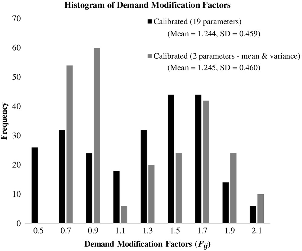
There was no major difference in the time it took to run the original (e.g., 19 parameters) and the revised (e.g., 2 parameters) calibration procedure. This is not surprising because both used the same number of maximum iterations as the stopping criteria, and the extra step (e.g., identifying the 19 demand factors given a mean and variance of the DMF distribution) did not involve a significant amount of computing time. However, the revised calibration procedure was able to identify a statistically significant solution in the first iteration as compared to the fifth iteration in the original. In addition, the revised procedure identified 26, as opposed to 15, statistically valid solutions. It is easy to hypothesize that calibrating 2 parameters would be more efficient than calibrating 19 parameters, and this was found to be the case for this testbed.
As previously, the calibrated parameter set using the mean-and-variance process can be converted to a standardized bell-shaped histogram if the user desires. Alternatively, the calibration procedure could assume that there is an underlying PDF associated with the mean and variance identified from the GA. This could obviate the need to transform the demand factors, although this was not examined in this paper.
Concluding Remarks
This paper proposes a methodology for calibrating the HCM-6 TTR model so that it replicates an empirical TTD. It is expected that the proposed calibration approach will allow HCM-6 users to obtain accurate estimates of both the TTD and the associated TTR metrics.
A () principal arterial in Lincoln, Nebraska, was used as a testbed. The HCM-6 TTR model was calibrated using a genetic algorithm. The study made the following findings:
1.
There were statistically significant differences between the uncalibrated and the empirical TTDs at a 5% significance level. The uncalibrated HCM-6 TTR model resulted in a TTD that was highly peaked, and the standard deviation was 67% lower than that of the empirical data.
2.
There was an average of 3% error in the estimated TTD when the HCM-6 TTR model was calibrated compared to a 17% error when the TTD was not calibrated. More importantly, there were no statistically significant differences between the estimated TTD from the calibration process and the empirical TTD. However, on average the standard deviations of the accepted calibrated solution were 12% smaller than the empirical BT data. If this were a concern, it would be relatively easy to make this a part of the calibration process.
3.
Not surprisingly, the resultant TTR metrics of the calibrated conditions are all similar to field measurements. The uncalibrated condition tends to overestimate reliability performance measures. Consequently, the uncalibrated-condition TTR metrics show that the testbed is more reliable than what it should be in field measurements. The estimation errors for the travel time index, planning time index, and level of TTR were 3%, 18%, and 8%, respectively.
4.
It was shown that the mean and variance of the calibrated demand factors can be readily transformed into alternative distribution forms (e.g., bell-shaped) if the user desires. For the test example, this has no impact on the statistical significance of the results. However, this result may be application-specific.
In summary, the calibration process introduced more variability in the demand compared to the uncalibrated conditions. This increased variability resulted in a “better” fit to the empirical TTD. At first glance, the calibrated demand factors would appear to have no “physical” meaning. However, it is easy to show that the calibrated demand can be transformed into alternative forms. Note that the authors are not asserting that the calibrated demand factors accurately represent demand variation in the field. It is entirely plausible, and probably highly likely, that the changes in the demand factors may capture not only differences in demand but also the effects of other variables not considered in the HCM-6 TTR procedure.
It must be noted that the calibration results presented are only valid for the city of Lincoln, on one corridor, and for a 1-year reliability reporting period. However, as more corridors’ travel information becomes available, the calibration methodology may be repeated. This will allow users to determine whether there is any commonality in the calibrated parameter sets, which could then be published in future HCM editions.
The authors also recommend that the HCM developers examine whether the large discrepancies found in this paper apply to other locations in the United States. If so, the authors suggest a reexamination of the TTR methodology to determine whether there are missing variables that should be included.
Future studies will focus on the temporal and spatial transferability of calibrated model parameters. Intuitively, this will help save the time cost of modeling and calibrating all arterials in a network. In addition, it will guide the conditions necessary or appropriate when transferring the HCM-6 calibrated model parameters.
Data Availability Statement
Some or all data, models, or code used during the study were provided by a third party (testbed demand and supply data). Direct requests for these materials may be made to the provider as indicated in the acknowledgments.
Acknowledgments
The authors would like to thank the City of Lincoln for making local data readily available. The contents of this paper reflect the views of the authors, who are responsible for the facts and accuracy of the information presented herein and are not necessarily representative of the state of Nebraska or the city of Lincoln. The authors appreciate the assistance of Andy Jenkins of the City of Lincoln for readily providing testbed data and James Bonneson of Kittleson and Associates who graciously shared his expertise on how the HCM-6 TTR model was developed.
References
Agdas, D., D. J. Warne, J. Osio-Norgaard, and F. J. Masters. 2018. “Utility of genetic algorithms for solving large-scale construction time-cost trade-off problems.” J. Comput. Civ. Eng. 32 (1): 04017072. https://doi.org/10.1061/(ASCE)CP.1943-5487.0000718.
Angelova, M., and T. Pencheva. 2011. “Tuning genetic algorithm parameters to improve convergence time.” Int. J. Chem. Eng. 2011: 1–7. https://doi.org/10.1155/2011/646917.
Appiah, J., B. Naik, L. Rilett, Y. Chen, and S.-J. Kim. 2011. Development of a state of the art traffic microsimulation model for Nebraska. Lincoln, NE: Nebraska DOT.
Arezoumandi, M., and G. H. Bham. 2011. “Travel time reliability estimation: Use of median travel time as measure of central tendency.” In Proc., Transportation and Development Institute Congress 2011: Integrated Transportation and Development for a Better Tomorrow, 59–68. Reston, VA: ASCE. https://doi.org/10.1061/41167(398)7.
Bonneson, J. A. 2014. Urban street reliability engine user guide. Mountain View, CA: Kittelson & Associates.
Cambridge Systematics. 2005. Traffic congestion and reliability: Trends and advanced strategies for congestion mitigation. Washington, DC: Federal Highway Administration.
Cimorelli, L., A. D’Aniello, and L. Cozzolino. 2020. “Boosting genetic algorithm performance in pump scheduling problems with a novel decision-variable representation.” J. Water Resour. Plann. Manage. 146 (5): 04020023. https://doi.org/10.1061/(ASCE)WR.1943-5452.0001198.
Cotten, D., J. Codjoe, and M. Loker. 2020. “Evaluating advancements in Bluetooth technology for travel time and segment speed studies.” Transp. Res. Rec. 2674 (4): 193–204. https://doi.org/10.1177/0361198120911931.
Datta, S. K., R. P. F. Da Costa, J. Härri, and C. Bonnet. 2016. “Integrating connected vehicles in Internet of Things ecosystems: Challenges and solutions.” In Proc., 2016 IEEE 17th Int. Symp. on a World of Wireless, Mobile and Multimedia Networks (WoWMoM), 1–6. New York: IEEE.
Dowling, R. G., A. Skabardonis, R. A. Margiotta, and M. E. Hallenbeck. 2009. Reliability breakpoints on freeways. Washington, DC: Transportation Research Board.
FHWA and USDOT (Federal Highway Administration and USDOT). 2012. “Moving ahead for progress in the 21st century.” Accessed December 9, 2019. http://www.fhwa.dot.gov/map21/.
FHWA and USDOT (Federal Highway Administration and USDOT). 2015. “Fixing America’s surface transportation act.” Accessed December 9, 2019. http://www.fhwa.dot.gov/fastact/.
FHWA Office of Operations and US DOT. 2017. “Travel time reliability: Making it there on time, all the time.” Accessed August 23, 2019. https://ops.fhwa.dot.gov/publications/tt_reliability/TTR_Report.htm#Whatmeasures.
Figliozzi, M. A., N. Wheeler, E. Albright, L. Walker, S. Sarkar, and D. Rice. 2011. “Algorithms for studying the impact of travel time reliability along multisegment trucking freight corridors.” Transp. Res. Rec. 2224 (1): 26–34. https://doi.org/10.3141/2224-04.
Hassanat, A., K. Almohammadi, E. Alkafaween, E. Abunawas, A. Hammouri, and V. B. Prasath. 2019. “Choosing mutation and crossover ratios for genetic algorithms—A review with a new dynamic approach.” Information 10 (12): 390. https://doi.org/10.3390/info10120390.
Highway Capacity Manual. 2010. Transportation Research Board of the National Academies. Washington, DC: Transportation Research Board.
Highway Capacity Manual. 2016. A guide for multimodal mobility analysis. Washington, DC: Transportation Research Board.
INRIX. 2020. “Intelligence that moves the world.” Accessed February 12, 2020. https://inrix.com/about/.
Kim, S. J., W. Kim, and L. R. Rilett. 2005. “Calibration of microsimulation models using nonparametric statistical techniques.” Transp. Res. Rec. 1935 (1): 111–119. https://doi.org/10.1177/0361198105193500113.
Kochenderfer, M. J., and T. A. Wheeler. 2019. Algorithms for optimization. Cambridge, MA: MIT Press.
Kramer, O. 2017. Vol. 679 of Genetic algorithm essentials. New York: Springer.
Levinson, H. S., and R. Margiotta. 2011. “From congestion to reliability: Expanding the Horizon.” In Proc., Transportation and Development Institute Congress 2011: Integrated Transportation and Development for a Better Tomorrow, 1066–1074. Reston, VA: ASCE. https://doi.org/10.1061/41167(398)102.
Mahmassani, H. S., J. Kim, Y. Chen, Y. Stogios, A. Brijmohan, and P. Vovsha. 2014. Incorporating reliability performance measures into operations and planning modeling tools. Washington, DC: Transportation Research Board.
Pu, W. 2011. “Analytic relationships between travel time reliability measures.” Transp. Res. Rec. 2254 (1): 122–130. https://doi.org/10.3141/2254-13.
Roess, R. P., and E. S. Prassas. 2014. The Highway Capacity Manual: A conceptual and research history, 249–338. New York: Springer.
Roeva, O., and P. Vassilev. 2016. “InterCriteria analysis of generation gap influence on genetic algorithms performance.” In Novel developments in uncertainty representation and processing, 301–313. Cham, Switzerland: Springer.
Spiegelman, C., E. S. Park, and L. R. Rilett. 2010. Transportation statistics and microsimulation. Boca Raton, FL: CRC Press.
Tan, H., Q. Li, Y. Wu, B. Ran, and B. Liu. 2015. “Tensor recovery based non-recurrent traffic congestion recognition.” In Proc., CICTP 2015, 591–603. Reston, VA: ASCE. https://doi.org/10.1061/9780784479292.054.
Taylor, M. A. P. 2013. “Travel through time: The story of research on travel time reliability.” Transportmetrica B: Transport Dyn. 1 (3): 174–194. https://doi.org/10.1080/21680566.2013.859107.
Tufuor, E. O., and L. R. Rilett. 2018. Analysis of low-cost Bluetooth-plus-WiFi device for travel time research. Washington, DC: Transportation Research Board.
Tufuor, E. O., and L. R. Rilett. 2019. “Validation of the Highway Capacity Manual urban street travel time reliability methodology using empirical data.” Transp. Res. Rec. 2673 (4): 415–426. https://doi.org/10.1177/0361198119838854.
Tufuor, E. O., and L. R. Rilett. 2020. “Analysis of component errors in the Highway Capacity Manual travel time reliability estimations for urban streets.” Transp. Res. Rec. 2674 (6): 85–97. https://doi.org/10.1177/0361198120917977.
Van Lint, J. W. C., H. J. Van Zuylen, and H. Tu. 2008. “Travel time unreliability on freeways: Why measures based on variance tell only half the story.” Transp. Res. Part A: Policy Pract. 42 (1): 258–277. https://doi.org/10.1016/j.tra.2007.08.008.
Willmott, C. J., and K. Matsuura. 2005. “Advantages of the mean absolute error (MAE) over the root mean square error (RMSE) in assessing average model performance.” Clim. Res. 30 (1): 79–82. https://doi.org/10.3354/cr030079.
Yang, L., X. Zhao, S. Peng, and X. Li. 2016. “Water quality assessment analysis by using combination of Bayesian and genetic algorithm approach in an urban lake, China.” Ecol. Modell. 339 (Nov): 77–88. https://doi.org/10.1016/j.ecolmodel.2016.08.016.
Yao, J., F. Shi, Z. Zhou, and J. Qin. 2012. “Combinatorial optimization of exclusive bus lanes and bus frequencies in multi-modal transportation network.” J. Transp. Eng. 138 (12): 1422–1429. https://doi.org/10.1061/(ASCE)TE.1943-5436.0000475.
Zegeer, J., et al. 2014. Incorporating travel time reliability into the Highway Capacity Manual. Washington, DC: Transportation Research Board.
Information & Authors
Information
Published In

Journal of Transportation Engineering, Part A: Systems
Volume 146 • Issue 12 • December 2020
Copyright
This work is made available under the terms of the Creative Commons Attribution 4.0 International license, https://creativecommons.org/licenses/by/4.0/.
History
Received: Mar 31, 2020
Accepted: Jun 23, 2020
Published online: Sep 16, 2020
Published in print: Dec 1, 2020
Discussion open until: Feb 16, 2021
Authors
Metrics & Citations
Metrics
Citations
Download citation
If you have the appropriate software installed, you can download article citation data to the citation manager of your choice. Simply select your manager software from the list below and click Download.