Abstract
Real-time performance measures are important for agencies to maintain their roadways during the winter season. However, infrastructure can be expensive to deploy and maintain and may be sparse in rural areas, while speed data alone may not provide enough fidelity in borderline conditions. This study looks at high-frequency vehicle data from the in-vehicle bus to detect changes in the vehicle and driver behavior during changing winter road conditions. The data is reported to the cloud via cellular communication and is viewable in real-time using a map-based web dashboard. Three winter weather events are assessed using in-vehicle data collected from the February–March 2018 period. Using a two-sample Kolmogorov-Smirnov test, we found high significance in the reductions of applied brake pressures and rates of braking in winter versus fair weather conditions before vehicle intervention is necessary. The paper concludes that pairwise comparison of driver change in brake pressure may be a valuable data source indicative of deteriorating road conditions before more severe indicators such as traction control, antilock brake, and/or hazard indicators are activated.
Introduction
Winter road conditions are hazardous for drivers to navigate and are a challenge for agencies to manage. According to the US Federal Highway Administration’s (FHWA’s) Road Weather Management Program (RWMP), out of approximately 5,748,000 vehicle crashes each year, about 22% of these crashes are weather related (FHWA 2018). From 2005 to 2014, an average of 445,303 persons were injured and 5,897 persons were killed annually in weather-related crashes. Of these weather-related crashes, 17% of occurred during snow or sleet, 13% occurred on icy pavement, and 14% occurred on snowy or slushy pavement. The estimated annual cost of weather-related crashes ranges from $22 to $51 billion (Pisano et al. 2008). Additionally, it is estimated that weather-related delays cost the trucking industry about $8 to $9 billion annually (FHWA 2017a).
In 2015, the Road Weather Management Performance Measures report (FHWA 2015) evaluated a set of 27 performance measures aimed to assess the status of the transportation system during inclement winter weather conditions. The objectives identified in an updated report (FHWA 2017b) included “advancement of the state of the art for mobile sensing and integrating vehicle data into road weather applications,” and “improve integration of weather-related decision-support technologies into traffic operations and maintenance procedures.”
Vehicle Data
Before the advent of onboard vehicle communication electronics in the late 1980s (McMillan 1984; Cox 1984), it was difficult to obtain any type of vehicle telematics data without dedicated instrumentation. However, modern vehicles have come equipped with localized networks that facilitate communication between the various onboard components (Kiencke et al. 1986), and report vehicle dynamics information such as wheel speed, engine controls, drivetrain, and brake pressures at subsecond frequencies. The data are typically used for controlling and coordinating vehicle features such as traction control and antilock braking systems [Gerstenmeier and Weber 1987; Antilock Braking System, “Teldix,” UK Patent No. 1,245,620 (1971)]. However, if the same data were to be packaged and delivered via a system that can integrate with data-driven software interfaces to generate weather-related performance measures using modern-day cellular networks, it can provide tremendous value to stakeholders and agencies. A previous study has shown that using segment-based connected vehicle data, speed drops can be used to detect inclement weather conditions and recommend winter maintenance strategies (Hainen et al. 2012). Expanding on this concept, because modern production vehicles can be used to detect loss of friction conditions using signals from integrated onboard components (Zhao et al. 2014; Casselgren 2018), and if the data can be harvested and calibrated using high-fidelity data logging instruments and crowdsourcing, may have potential to achieve the objectives outlined by the 2015 RWMP (FHWA 2015).
Methodology
This study developed methods to extract on board vehicle data to assess whether current vehicle technologies can provide informative road condition data during winter storms.
Data System
The experimental setup (Fig. 1) was comprised of a series production vehicle (2017 Audi A4 Allroad) and a laptop. Each test was performed with one occupant (the driver), and no additional loading. The brake pad and rotors were in good condition [under 16,000 km (10,000 mi)] and tire pressures were checked before each test. The vehicle comes with a build-in wireless internet access point. A laptop was placed in the trunk with an inexpensive controller area network universal serial bus (CANUSB) device, which is a device that feeds the controller area network (CAN) signals forwarded from the various communication buses in the vehicle to the laptop, and is natively supported in Linux as a socket (Hartkopp 2012).
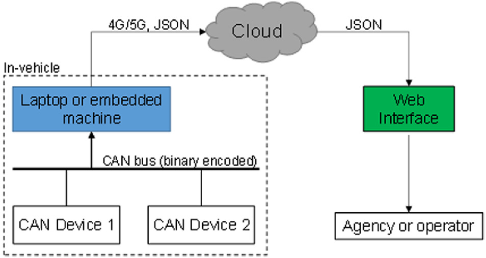
The laptop was used to decode and record the following CAN signals: antilock brake (ABS) activation, traction-control intervention, wheel ticks, hazard lights, windshield wiper state, and brake pressure. Depending on the bus on which the device is emitting, the frequency of the signal can be anywhere between 100 and 200 milliseconds (ms). Once a notable status change of the identified signal was detected, the signal was uploaded with a time stamp, together with a global positioning system (GPS) point where the change occurred, to a secure server via the onboard internet access point. The message was a hypertext transfer protocol (HTTP) post (Fielding 1996) and encoded as a JavaScript object notation (JSON) message (Bray 2014) sent through the cloud. Through a web interface, the server then processed the message and stored the signal into an structured query language (SQL) database. The laptop also had the ability to store the selected in-vehicle signals as comma-separated variable (CSV) files instead of uploading to the cloud.
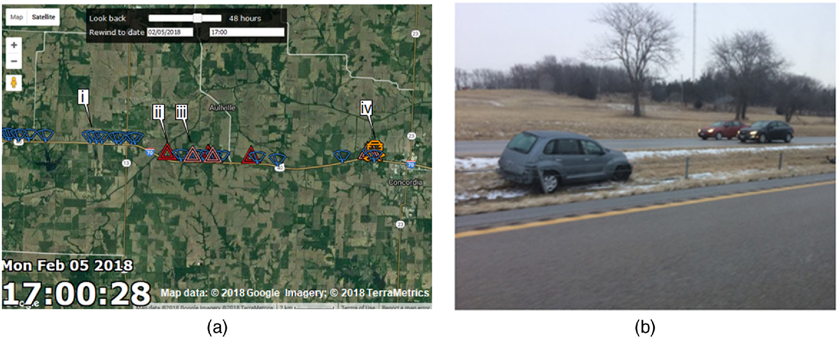
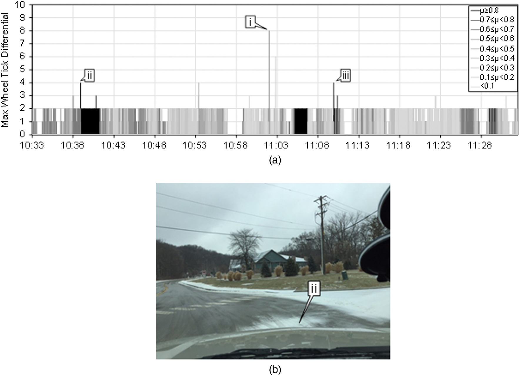
A web dashboard was developed to verify the uploaded vehicle signals in the database. Fig. 2(a) shows a dashboard interface on a Google Maps graphical layer. The windshield wiper (Callout i), hazard light activation (Callouts ii and iii), and traction control (Callout iv) signals from the test vehicle were plotted as they were received while traveling eastbound on I-70 during a winter storm on February 5, 2018 in central Missouri. According to local reports, heavy snowfall and icing on the roadways caused over 650 crashes [Fig. 2(b)] and multiple fatalities. The interface also has the ability to look at historic events.
User Road Condition Rating
A dashboard camera captured images from the forward view of the vehicle at 5-s intervals and the road condition was then assessed based on a qualitative rating scale by the driver. The ratings are as follows: a rating of 1 is dry or slightly damp where the driver would expect good friction; a rating of 2 is wet and the driver expects slightly slippery conditions; and pa rating of 3 is where there is snow or slush and where the driver would expect some sliding with a hard maneuver. Because the driver was not able to record the observation during the drives, this was performed as an after-action assessment. User ratings were recorded using software that displays an image from the experiments at random and records the user rating input. Over 9,000 images from the experiments were assessed.
Mobile Road Weather Information Sensor
Friction data was collected using a mobile road weather information sensor (MARWIS) system. The sensor was mounted on the rear of a chase vehicle about 1 m (3 ft) above the pavement surface. The coefficient of friction () measured from the road surface condition was averaged and recorded at 10-s intervals. The friction estimates and based on lasers have relatively low fidelity, but these devices are commonly used by highway agencies as mobile probes during winter storms. The geographic location of the friction data was also saved using the associated GPS reported from the MARWIS device.
Wheel Ticks
Modern vehicles are equipped with wheel speed sensors (Hartley 1974) that report the position of each wheel as an integer, such as in the range of 0 to 1,000, to the various onboard control units and devices via the in-vehicle bus [T. Svantesson, “Detection of short term irregularities in a road surface,” US Patent No. 14,913,684 (2015)]. As the vehicle moves, the integer position, or wheel tick, increments at a rate equal to the angular velocity of each wheel. The number is reset to 0 once it reaches the maximum within its allocated range (). Depending on the vehicle’s equipment, the range of the integer and the rotation angle per unit can be different. The data collection system used in this study recorded the wheel tick value of each wheel at a rate of 100 ms. To estimate the angular velocity of one wheel, the difference between two consecutive wheel tick values and are usedwhere = angular velocity in wheel ticks per second. The angular velocities of all four wheels of the vehicle were measured using this method and recorded at each time interval to check for large discrepancies.
(1)
Because the wheels on a vehicle travel at different velocities while turning due to the difference of the inner and outer track radii, the discrepancies of the wheels across the front and rear axles were ignored. Only the differences along each side of the vehicle were assessed. Fig. 3(a) shows the recorded angular velocities of each wheel over a 3.4 s time interval during a deceleration event. The front driver (), front passenger (), rear driver (), and rear passenger () angular velocities are plotted on the graph. Between 02:49.9 and 02:50.2, a noticeable divergence in wheel speed is evident for the front passenger wheel. This wheel started to travel slower than the other three wheels, and at Callout i in Fig. 3(a) this was most pronounced. The angular velocity difference () along each side of the vehicle is computed as follows:
(2)
(3)
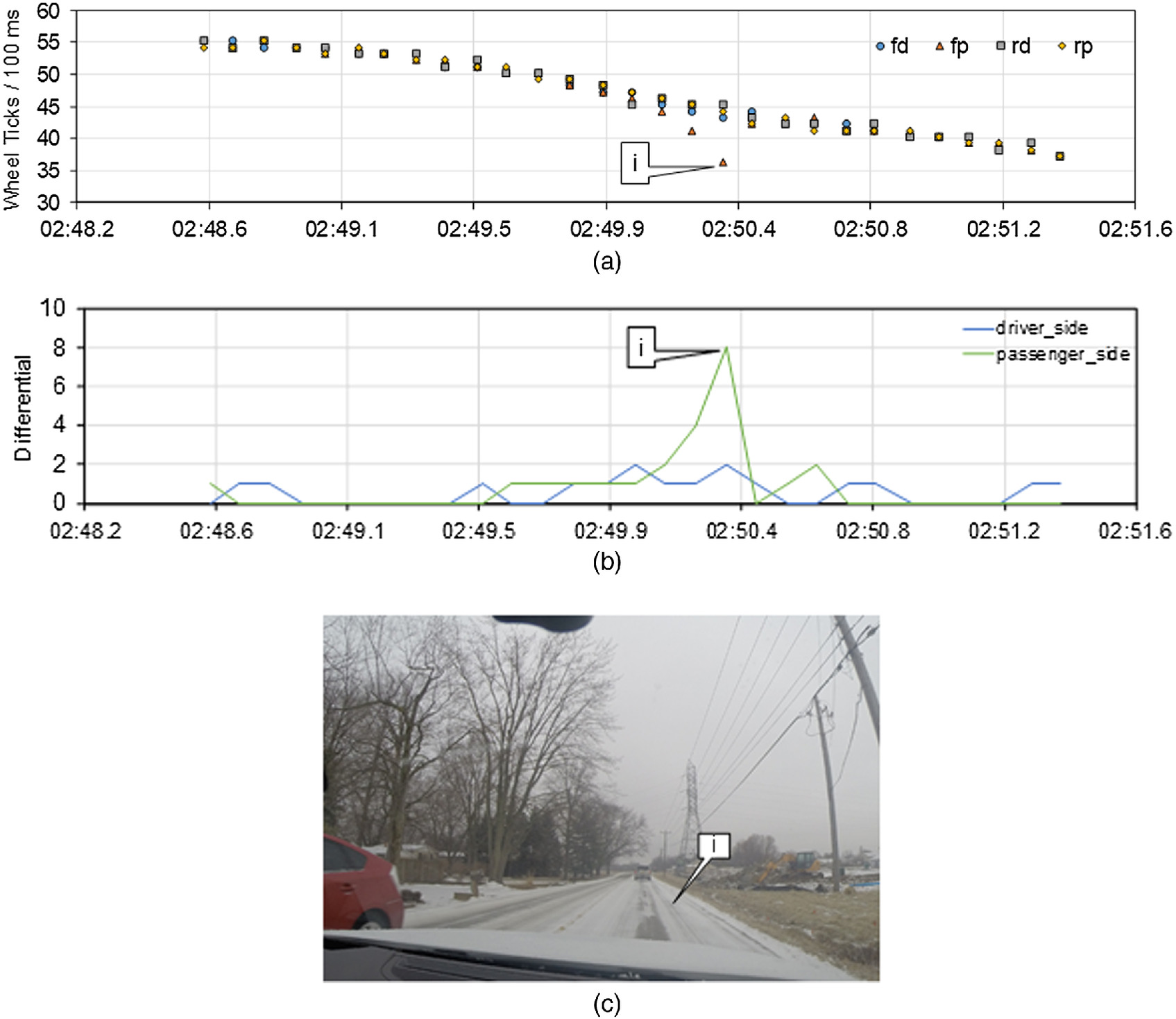
Fig. 3(b) plots the differences along each side of the vehicle. The greatest value was recorded at 02:50.3 with an absolute difference of eight wheel ticks between the front passenger and rear passenger wheels [Fig. 3(b), Callout i]. This was associated with a braking event before a stop sign that triggered an ABS intervention by the vehicle [Fig. 3(c), Callout i].
Braking
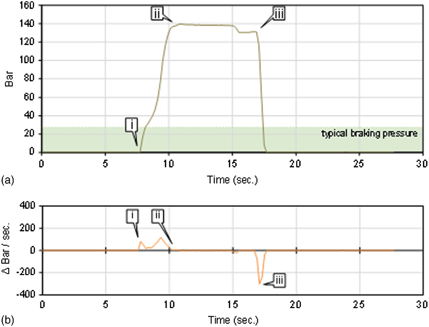
The amount of braking applied was measured using static brake line pressures sampled in bar units from the vehicle bus at 200-ms intervals. Fig. 4(a) shows a profile of the pressure during a test procedure where the brake was applied with heavy force over a 10-s interval with the vehicle parked. Callout i indicates the moment when the brake was first applied. The force hit a maximum value of 140 bars at Callout ii and was released at Callout iii. Typical braking pressures from the winter driving conditions tested in this study were recorded to be under 25 bars.
In addition to static pressure, the change in pressure () can also be calculated over two consecutive data samples and to measure the rate at which the driver applies or releases braking force
(4)
Fig. 4(b) plots the change in braking pressure in the same braking test. Two rapid changes in brake application were detected during the experiment as indicated by Callout i about 7–10 s into the experiment. The change in brake pressure reached 53 and in each of the peaks, respectively. The braking force was held constant between 10 and 17 s, which reflects a zero value for the rate of change (Callout ii). At Callout iii, the brake was rapidly released and registered a rate of . A benefit of using change in brake pressure over static brake pressure is that it is able to characterize the speed at which the brake pedal is applied and released.
Data Collection
Test Circuit Road Conditions
The test vehicle was driven in a predetermined loop of 11.3 km in the area around West Lafayette, IN. The experiment was repeated on four different days with different conditions in 2018:
•
February 11 (icy),
•
March 24 (dry to snowy),
•
July 4 (dry and sunny), and
•
July 9 (dry and sunny).
On February 11, the test started and ended in icy conditions. On March 24, the test circuit was dry at the beginning of the day and became snow covered and slippery as the day progressed. In the days with winter conditions, a separate vehicle with a MARWIS pavement friction sensor was also included. Two drivers were assigned to a pair of winter and dry condition days; one driver for February 11 and July 9, and the other driver for March 24 and July 4. The drivers were aware and consented to the data collection, and were told to drive normally as they would under each weather condition. The experiments collected measurements from multiple in-vehicle bus signals, and were repeated along the same road links in the test loop per day. This was to essentially emulate fleet data as time progressed. For example, using vehicle count data from traffic signal controller event logs, the runs were approximately 2% of the total volume for March 24.
Map Segmentation
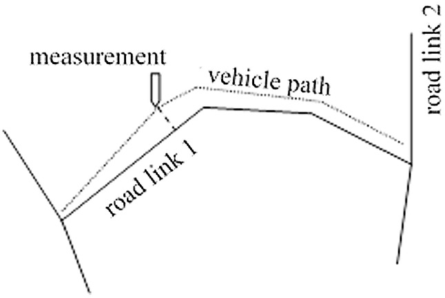
The vehicle provided a constant stream of wheel ticks from which the differential angular velocity from the same side of the vehicle was calculated. Each data point is also associated with a GPS coordinate identifying the vehicle’s position. In order to visualize the segment of roadway affected with the highest slip differentials, the measured data was attributed to a road link. This process would also help hide precise locations for future use cases where privacy is a concern. Moreover, GPS coordinates are not always perfectly aligned with the road. In order to match measurements of repeated passes to a road, links from a HERE Global B.V navigation map were leveraged for this study. Road links consist of geometrical lines defined by several latitude and longitude points. Each road link has a unique identifier with starting and ending points along the roadway. The measurement of the vehicle was mapped to the nearest road link identifier using a perpendicular distance (dashed line in Fig. 5). If multiple slip measurements fall onto the same road link, they are averaged. The 48-road links used for this study are shown in Table 1.
| Link ID | Length (km) | Limit () | End of segment | Movement | Link ID | Length (km) | Limit () | End of segment | Movement |
|---|---|---|---|---|---|---|---|---|---|
| 1 | 0.19 | 80 | No control | Though | 25 | 0.04 | 32 | No control | Through |
| 2 | 0.20 | 80 | No control | Right turn | 26 | 0.04 | 32 | No control | Through |
| 3 | 0.20 | 64 | No control | Through | 27 | 0.27 | 32 | Yield | Roundabout |
| 4 | 0.19 | 64 | No control | Through | 28 | 0.05 | 32 | No control | Through |
| 5 | 0.36 | 64 | Stop sign | Through | 29 | 0.10 | 56 | No control | Through |
| 6 | 0.21 | 64 | Stop sign | Right turn | 30 | 0.04 | 56 | No control | Through |
| 7 | 0.24 | 64 | No control | Through | 31 | 0.05 | 56 | No control | Through |
| 8 | 0.20 | 64 | No control | Through | 32 | 0.06 | 56 | No control | Through |
| 9 | 0.16 | 64 | No control | Through | 33 | 0.09 | 56 | No control | Through |
| 10 | 0.15 | 64 | No control | Through | 34 | 0.40 | 64 | Signal | Right turn |
| 11 | 0.08 | 64 | No control | Through | 35 | 2.56 | 88 | Signal | Left turn |
| 12 | 0.62 | 80 | No control | Through | 36 | 0.12 | 64 | No control | Through |
| 13 | 0.16 | 64 | No control | Through | 37 | 0.01 | 80 | Signal | Through |
| 14 | 0.26 | 64 | No control | Through | 38 | 0.12 | 56 | No control | Through |
| 15 | 0.12 | 56 | No control | Through | 39 | 0.02 | 80 | Signal | Through |
| 16 | 0.15 | 56 | No control | Through | 40 | 1.21 | 80 | Signal | Left turn |
| 17 | 0.27 | 56 | Signal | Through | 41 | 0.52 | 80 | Signal | Through |
| 18 | 0.09 | 56 | No control | Through | 42 | 0.01 | 80 | No control | Through |
| 19 | 0.07 | 56 | No control | Through | 43 | 0.42 | 56 | Signal | Right turn |
| 20 | 0.08 | 56 | Signal | Right turn | 44 | 0.03 | 32 | Roundabout | Roundabout |
| 21 | 0.05 | 56 | No control | Through | 45 | 0.01 | 32 | Roundabout | Roundabout |
| 22 | 0.16 | 56 | No control | Through | 46 | 0.04 | 32 | No control | Roundabout |
| 23 | 0.30 | 80 | No control | Through | 47 | 0.30 | 80 | No control | Through |
| 24 | 0.24 | 80 | No control | Through | 48 | 0.04 | 80 | No control | Through |
Friction Data
Road surface friction data was collected by a chase vehicle equipped with a MARWIS sensor. Using the map segmentation scheme described in Table 1, the pavement friction measurements were averaged into 15-min bins and assigned to the closest road link from the vehicle at that moment in time. In general, the friction estimates provide reasonable overall segment characterization of friction ranges, but do not have the fidelity to identify localized very short segments with low friction.
An table of friction values for the experiment conducted on March 24 is shown in Table 2. A dash ("—") indicates locations and time bins where no data was collected. On that day, at around 10:15 the coefficient of friction () on the test loop begins to drop below 0.8 due to accumulating snowfall for most links. The links that had the lowest detected friction values were 11 and 34. By 14:00, recovers to above 0.7 for most links in the loop.
| Link ID | 8:45 | 9:00 | 9:15 | 9:30 | 9:45 | 10:00 | 10:15 | 10:30 | 10:45 | 11:15 | 11:45 | 12:00 | 12:15 | 12:30 | 12:45 | 13:00 | 13:15 | 13:30 | 13:45 | 14:00 | 14:15 |
|---|---|---|---|---|---|---|---|---|---|---|---|---|---|---|---|---|---|---|---|---|---|
| 1 | — | 0.82 | 0.82 | 0.82 | 0.82 | 0.82 | 0.76 | 0.73 | — | — | — | 0.73 | 0.73 | 0.72 | 0.75 | 0.74 | 0.75 | 0.75 | 0.76 | 0.76 | 0.76 |
| 2 | — | 0.82 | 0.82 | 0.82 | 0.82 | 0.82 | 0.76 | 0.75 | — | — | — | 0.73 | 0.69 | 0.72 | 0.70 | 0.73 | 0.71 | 0.74 | 0.75 | 0.74 | 0.76 |
| 3 | — | — | — | 0.82 | 0.82 | 0.82 | 0.80 | 0.56 | — | — | — | 0.75 | — | 0.65 | 0.68 | 0.69 | 0.73 | 0.70 | 0.73 | 0.77 | 0.77 |
| 4 | — | — | — | 0.82 | 0.82 | 0.82 | 0.80 | 0.70 | — | — | — | 0.76 | 0.67 | 0.65 | 0.65 | 0.74 | 0.71 | 0.73 | 0.76 | 0.77 | 0.77 |
| 5 | — | — | — | 0.82 | 0.82 | 0.81 | 0.79 | 0.68 | — | — | — | 0.75 | 0.59 | 0.64 | 0.67 | 0.65 | 0.66 | 0.66 | 0.77 | 0.78 | 0.78 |
| 6 | — | — | — | 0.82 | 0.82 | 0.82 | 0.79 | 0.71 | — | — | — | 0.71 | 0.65 | 0.63 | 0.69 | 0.61 | 0.62 | 0.66 | 0.76 | 0.75 | 0.78 |
| 7 | — | — | — | 0.82 | 0.82 | 0.82 | 0.80 | 0.76 | — | — | — | 0.76 | 0.74 | 0.63 | 0.69 | 0.75 | 0.69 | 0.72 | 0.76 | 0.76 | 0.71 |
| 8 | — | 0.82 | — | 0.82 | 0.82 | 0.81 | 0.80 | 0.78 | — | — | — | 0.76 | 0.66 | 0.69 | 0.63 | 0.74 | 0.75 | 0.73 | 0.76 | 0.77 | |
| 9 | — | 0.82 | — | 0.82 | 0.82 | 0.82 | 0.78 | 0.73 | — | — | — | 0.72 | 0.66 | 0.58 | 0.69 | 0.61 | 0.68 | 0.76 | 0.72 | 0.78 | 0.79 |
| 10 | — | 0.82 | 0.82 | 0.82 | 0.82 | 0.82 | 0.78 | 0.74 | — | — | — | 0.76 | 0.66 | 0.58 | 0.74 | 0.70 | 0.67 | 0.77 | 0.77 | 0.76 | 0.77 |
| 11 | — | — | — | 0.82 | 0.82 | 0.81 | 0.79 | 0.62 | — | — | — | 0.66 | 0.67 | 0.64 | 0.64 | 0.46 | 0.48 | 0.58 | 0.68 | 0.75 | 0.76 |
| 12 | 0.82 | 0.82 | 0.82 | 0.82 | 0.82 | 0.82 | 0.80 | 0.75 | — | — | — | 0.75 | 0.75 | 0.75 | 0.77 | 0.76 | 0.75 | 0.75 | 0.75 | 0.76 | 0.77 |
| 13 | 0.82 | 0.82 | 0.82 | 0.82 | 0.82 | 0.82 | 0.78 | 0.75 | — | — | — | 0.74 | 0.74 | 0.73 | 0.76 | 0.77 | 0.73 | 0.75 | 0.76 | 0.77 | — |
| 14 | 0.82 | 0.82 | 0.82 | 0.82 | 0.82 | 0.82 | 0.80 | 0.75 | — | — | — | 0.74 | 0.74 | 0.74 | 0.74 | 0.76 | 0.72 | 0.74 | 0.76 | 0.76 | 0.77 |
| 15 | — | — | 0.82 | 0.82 | 0.82 | 0.82 | 0.82 | 0.79 | 0.76 | — | — | 0.79 | 0.77 | 0.80 | 0.81 | 0.81 | 0.79 | 0.74 | 0.79 | 0.82 | 0.80 |
| 16 | — | — | 0.82 | 0.82 | 0.82 | 0.82 | 0.82 | 0.80 | 0.76 | — | — | 0.78 | 0.79 | 0.79 | 0.80 | 0.80 | 0.79 | 0.78 | 0.81 | 0.81 | 0.81 |
| 17 | — | — | 0.82 | 0.82 | 0.82 | 0.82 | 0.81 | 0.80 | 0.76 | 0.76 | 0.76 | 0.76 | 0.77 | 0.78 | 0.79 | 0.81 | 0.76 | 0.74 | 0.77 | 0.78 | 0.82 |
| 18 | — | — | — | — | 0.82 | — | 0.82 | — | 0.76 | — | 0.77 | — | 0.77 | — | — | — | 0.77 | — | — | 0.79 | — |
| 19 | — | — | — | — | — | — | — | — | 0.78 | — | 0.77 | — | — | — | — | — | — | — | — | — | — |
| 20 | 0.82 | — | 0.81 | 0.82 | 0.82 | 0.82 | 0.81 | 0.76 | 0.73 | — | — | 0.74 | 0.74 | 0.75 | 0.76 | 0.77 | 0.77 | 0.76 | 0.79 | 0.78 | 0.81 |
| 21 | — | — | 0.81 | 0.82 | 0.82 | 0.82 | 0.81 | 0.77 | 0.73 | — | — | — | 0.73 | 0.78 | 0.76 | 0.77 | 0.77 | 0.76 | 0.79 | 0.78 | 0.81 |
| 22 | — | — | 0.82 | 0.82 | 0.82 | 0.82 | 0.82 | 0.79 | 0.78 | — | 0.77 | 0.80 | 0.79 | 0.78 | — | 0.78 | 0.77 | — | 0.78 | 0.78 | 0.77 |
| 23 | — | 0.82 | 0.82 | 0.82 | 0.82 | 0.82 | 0.79 | 0.75 | — | — | — | 0.75 | 0.73 | 0.74 | 0.77 | 0.76 | 0.74 | 0.73 | 0.73 | 0.73 | 0.74 |
| 24 | — | 0.82 | 0.82 | 0.82 | 0.82 | 0.82 | 0.78 | 0.74 | — | — | — | 0.76 | 0.75 | 0.73 | 0.76 | 0.76 | 0.75 | 0.76 | 0.75 | 0.75 | 0.77 |
| 25 | 0.82 | — | 0.82 | 0.82 | 0.82 | 0.82 | 0.80 | 0.79 | 0.76 | — | — | — | 0.77 | 0.78 | 0.77 | 0.79 | 0.69 | 0.74 | 0.79 | 0.79 | — |
| 26 | 0.82 | — | — | 0.82 | 0.82 | 0.82 | 0.80 | 0.76 | 0.76 | — | — | 0.78 | 0.77 | 0.78 | 0.77 | 0.79 | 0.77 | 0.74 | 0.79 | 0.79 | 0.81 |
| 27 | 0.82 | — | 0.82 | 0.82 | 0.82 | 0.82 | 0.80 | 0.76 | 0.77 | — | — | 0.75 | 0.76 | 0.74 | 0.77 | 0.76 | 0.74 | 0.77 | 0.78 | 0.78 | — |
| 28 | 0.82 | — | 0.82 | 0.82 | 0.82 | 0.81 | 0.79 | 0.77 | 0.78 | — | — | 0.78 | 0.77 | 0.78 | 0.78 | 0.76 | 0.70 | 0.78 | 0.79 | 0.79 | — |
| 29 | — | — | 0.82 | 0.82 | 0.82 | 0.82 | 0.82 | 0.80 | 0.74 | 0.76 | 0.71 | 0.76 | 0.71 | 0.72 | 0.79 | 0.75 | 0.74 | 0.74 | 0.77 | 0.77 | 0.81 |
| 30 | — | — | 0.82 | 0.82 | 0.82 | 0.82 | 0.82 | 0.79 | 0.77 | — | — | 0.79 | 0.77 | 0.76 | 0.81 | 0.78 | 0.74 | 0.74 | 0.80 | 0.81 | 0.81 |
| 31 | — | — | 0.82 | 0.82 | 0.82 | 0.82 | 0.81 | 0.79 | 0.78 | — | — | 0.81 | — | 0.80 | 0.81 | 0.80 | 0.80 | 0.78 | 0.81 | 0.81 | 0.82 |
| 32 | — | — | 0.82 | 0.82 | 0.82 | 0.82 | 0.81 | 0.77 | 0.75 | — | — | 0.77 | 0.77 | 0.78 | 0.80 | 0.77 | 0.79 | 0.79 | 0.80 | 0.78 | 0.81 |
| 33 | — | — | 0.82 | 0.82 | 0.82 | 0.82 | 0.81 | 0.77 | 0.75 | — | — | 0.81 | 0.77 | 0.79 | 0.80 | 0.79 | 0.79 | 0.79 | 0.80 | 0.81 | 0.82 |
| 34 | — | — | — | 0.82 | 0.82 | 0.82 | 0.79 | 0.66 | 0.59 | — | — | 0.60 | 0.64 | 0.62 | 0.53 | 0.62 | 0.72 | 0.67 | 0.75 | 0.77 | 0.77 |
| 35 | 0.82 | 0.82 | 0.82 | 0.82 | 0.82 | 0.82 | 0.79 | 0.76 | 0.71 | — | — | 0.76 | 0.75 | 0.74 | 0.75 | 0.76 | 0.73 | 0.74 | 0.78 | 0.78 | 0.79 |
| 36 | 0.82 | 0.82 | 0.82 | 0.82 | 0.82 | 0.82 | 0.78 | 0.77 | 0.71 | — | — | 0.75 | 0.72 | 0.73 | 0.78 | 0.77 | 0.74 | 0.67 | 0.77 | 0.72 | 0.77 |
| 37 | 0.82 | 0.82 | 0.82 | 0.82 | 0.82 | 0.82 | 0.78 | 0.76 | 0.71 | — | — | 0.76 | 0.72 | 0.73 | 0.73 | 0.75 | 0.73 | 0.67 | 0.76 | 0.72 | 0.77 |
| 38 | — | 0.82 | 0.82 | 0.82 | 0.82 | 0.81 | 0.78 | 0.76 | 0.76 | — | 0.77 | 0.78 | 0.72 | 0.71 | 0.73 | 0.75 | 0.71 | 0.74 | 0.76 | 0.78 | 0.77 |
| 39 | — | 0.82 | — | 0.82 | 0.82 | 0.82 | 0.81 | 0.79 | 0.74 | 0.77 | — | — | — | — | 0.77 | 0.78 | 0.77 | 0.77 | 0.79 | 0.79 | — |
| 40 | 0.82 | 0.82 | 0.82 | 0.82 | 0.82 | 0.82 | 0.80 | 0.77 | 0.71 | 0.77 | — | 0.77 | 0.72 | 0.76 | 0.77 | 0.77 | 0.76 | 0.76 | 0.78 | 0.79 | 0.79 |
| 41 | 0.82 | 0.82 | 0.82 | 0.82 | 0.82 | 0.82 | 0.80 | 0.78 | 0.76 | 0.77 | — | 0.77 | 0.78 | 0.74 | 0.77 | 0.76 | 0.77 | 0.77 | 0.78 | 0.78 | — |
| 42 | 0.82 | 0.82 | 0.82 | 0.82 | 0.82 | 0.81 | 0.79 | — | 0.76 | — | — | 0.77 | 0.78 | 0.77 | 0.79 | 0.76 | 0.77 | 0.77 | 0.78 | 0.75 | — |
| 43 | 0.82 | 0.82 | 0.82 | 0.82 | 0.82 | 0.82 | 0.79 | 0.76 | 0.75 | — | — | 0.77 | 0.75 | 0.77 | 0.77 | 0.77 | 0.75 | 0.77 | 0.77 | 0.78 | — |
| 44 | 0.82 | — | 0.82 | 0.82 | 0.82 | 0.82 | 0.80 | 0.76 | 0.76 | — | — | 0.78 | 0.77 | 0.77 | 0.77 | 0.77 | 0.77 | 0.78 | 0.78 | — | |
| 45 | 0.82 | — | 0.82 | 0.82 | 0.82 | 0.82 | 0.80 | 0.76 | 0.76 | — | — | 0.78 | 0.78 | 0.77 | 0.77 | 0.77 | 0.77 | 0.77 | 0.78 | 0.78 | — |
| 46 | 0.82 | — | 0.82 | 0.82 | 0.82 | 0.82 | 0.79 | 0.78 | 0.76 | — | — | 0.77 | 0.75 | 0.78 | 0.77 | 0.78 | 0.77 | 0.77 | 0.78 | 0.78 | — |
| 47 | — | 0.82 | 0.82 | 0.82 | 0.82 | 0.82 | 0.79 | 0.74 | — | — | — | 0.76 | 0.75 | 0.73 | 0.75 | 0.77 | 0.75 | 0.75 | 0.75 | 0.76 | 0.79 |
| 48 | — | 0.82 | 0.82 | 0.82 | 0.82 | — | 0.79 | 0.75 | — | — | — | 0.76 | 0.75 | 0.74 | 0.77 | 0.76 | 0.74 | 0.73 | 0.73 | 0.73 | 0.74 |
Wheel Slip
In contrast to MARWIS data, wheel slip can provide very high-fidelity information on location where low friction levels result in vehicle wheels sliding. In this study, wheel slippage is calculated using the wheel tick method, and is defined by the maximum absolute differential angular velocity of the front and rear wheels on either side of the vehicle. Fig. 6(a) shows a time series plot of the max wheel tick differential during the experiment conducted on February 11. The data is also colorized in grayscale using values collected from the MARWIS device (darker colors indicating higher friction values). Callout i indicates the wheel slip event from the example in Fig. 3(b) with the maximum differential value of 8. This was also where the ABS intervened on an approach to a stop sign, and corresponded to a value of 0.6 to 0.7.
Callouts ii and iii indicate locations where there was a high segment friction value reported by the MARWIS unit, but had some slip among the wheels. Inspecting these locations from photos found isolated patches of snow or ice [Fig. 6(b), Callout ii] that the vehicle likely slipped on but were not identified from the friction data. These discrepancies were due to the time-resolution and difference in sensing technology between the MARWIS lasers and wheel rotation data. High wheel rotation differentials were only detected when the vehicle was braking or accelerating hard in slippery areas, such as during the approach to or departing from an intersection. However, under unfavorable road conditions a driver may be less inclined to perform aggressive maneuvers like they would in dry conditions to intentionally prevent wheel slip. It is impractical to assume that as conditions deteriorate, drivers would proportionally increase the vehicle slip, and therefore this is an inconclusive metric for actual road conditions. As shown by the data from February 11, this may be how the driver behaved in this case. A related but more promising method uses wheel vibrations [T. Svantesson, “Detection of short term irregularities in a road surface,” US Patent No. 14,913,684 (2015)] which we may investigate in future research.
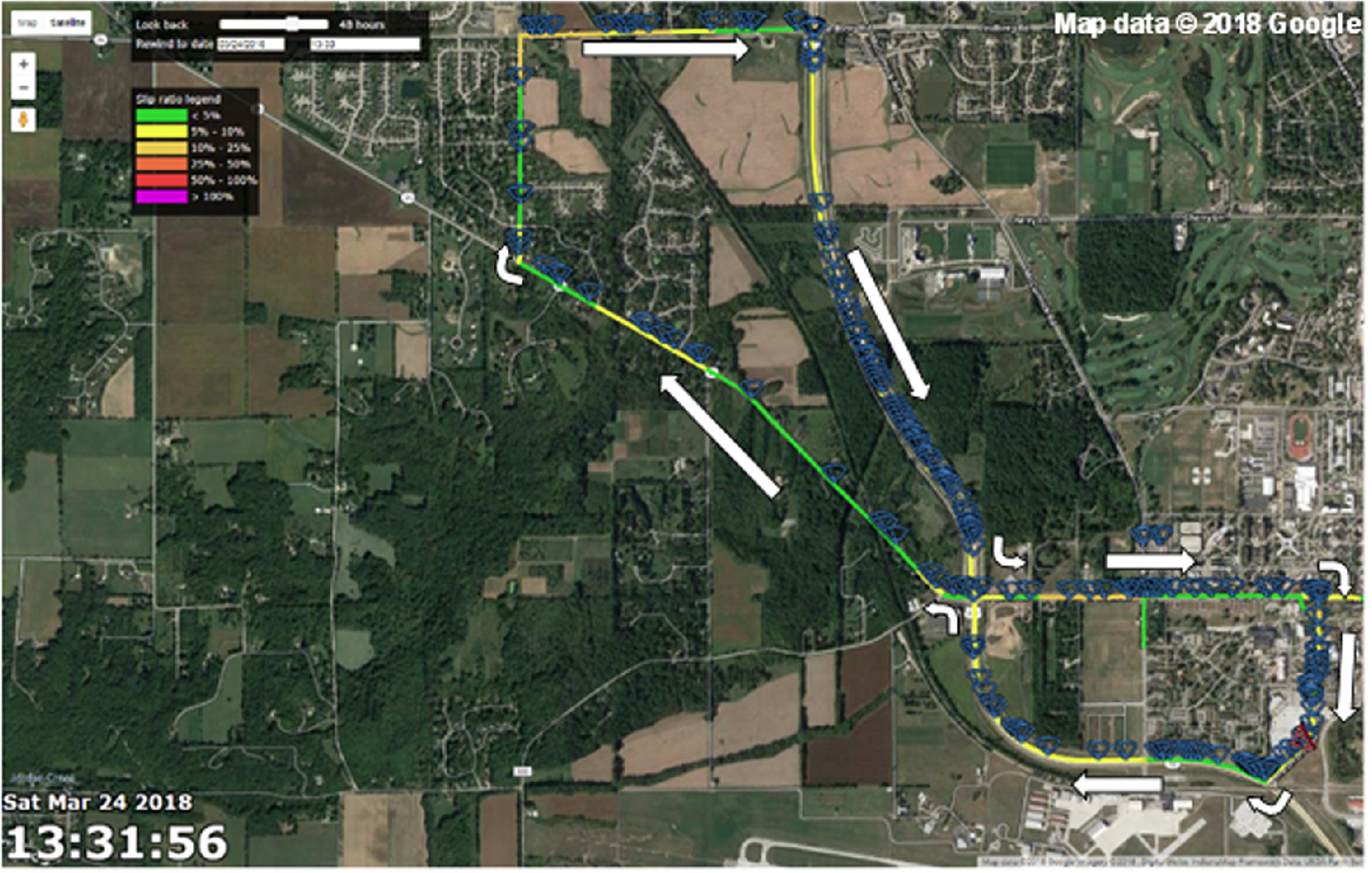
The maximum absolute differential angular velocity of one wheel can be converted to a slip percent by dividing it by the average angular velocities of the other wheels not experiencing slippage. The resulting value can be colorized based on a gradient scale and plotted on a map based on the segmentation scheme defined in Table 1. The map shown in Fig. 7 represents the slip percentages during the drive on March 24 at 13:31. Each link is assigned a color based on the last slip percentage value recorded on that link. The direction of vehicle travel is shown by the white arrows.
Braking
Static brake pressure (bar) and change in brake pressure () were recorded in each experiment to determine if a driver changed his braking behavior based on actual road conditions. Fig. 8 shows the user road condition rating [Fig. 8(a)], friction [Fig. 8(b)], speed [Fig. 8(c)], static brake pressure [Fig. 8(d)], and change in brake pressure [Fig. 8(e)] from the experiment conducted on March 24 for Link 34 of the test loop. As indicated in Table 2, the link experienced substantial drops in friction over the middle of the day. The data for all 18 passes at this location were combined together, and each sequential data point was assigned a time index. Photos from the dashboard camera corresponding to notable time indices are shown in Fig. 9. The condition at the beginning of the test was dry with good friction as indicated by Fig. 9(a).
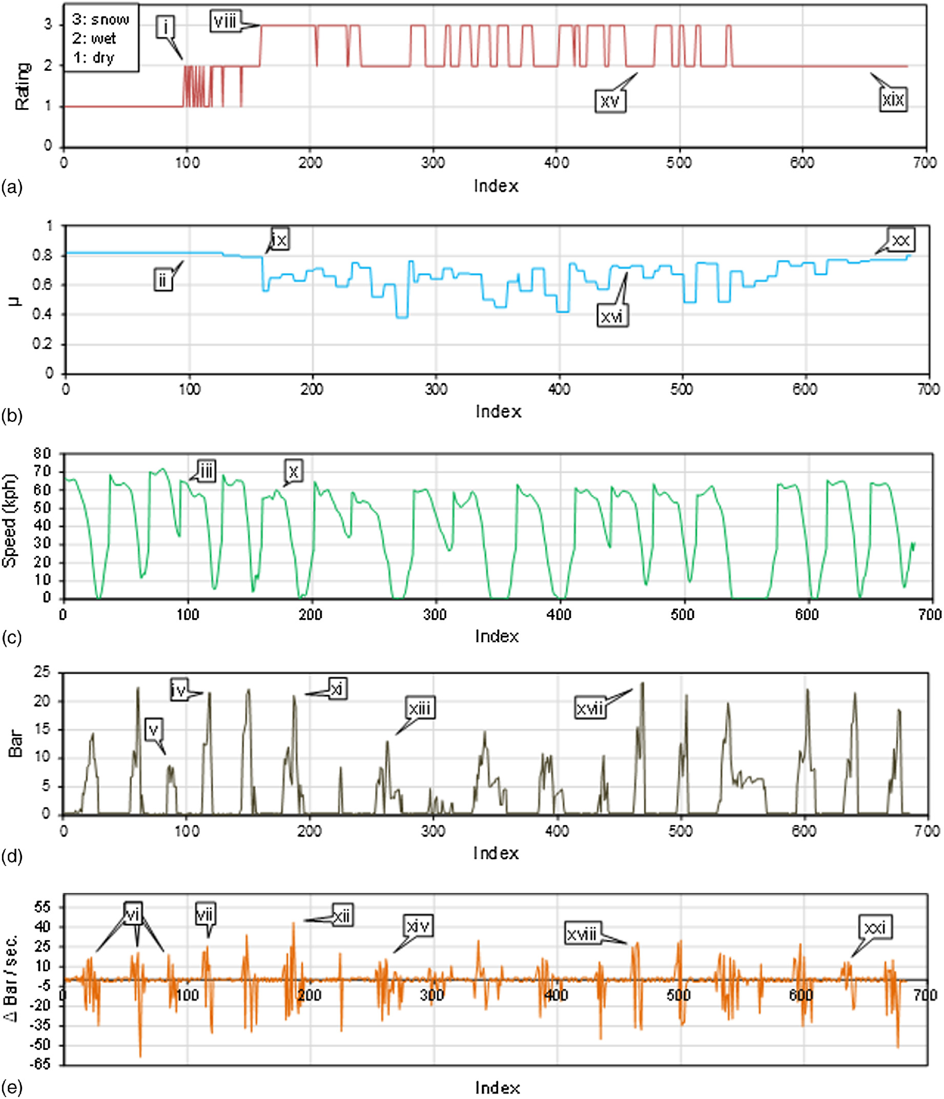
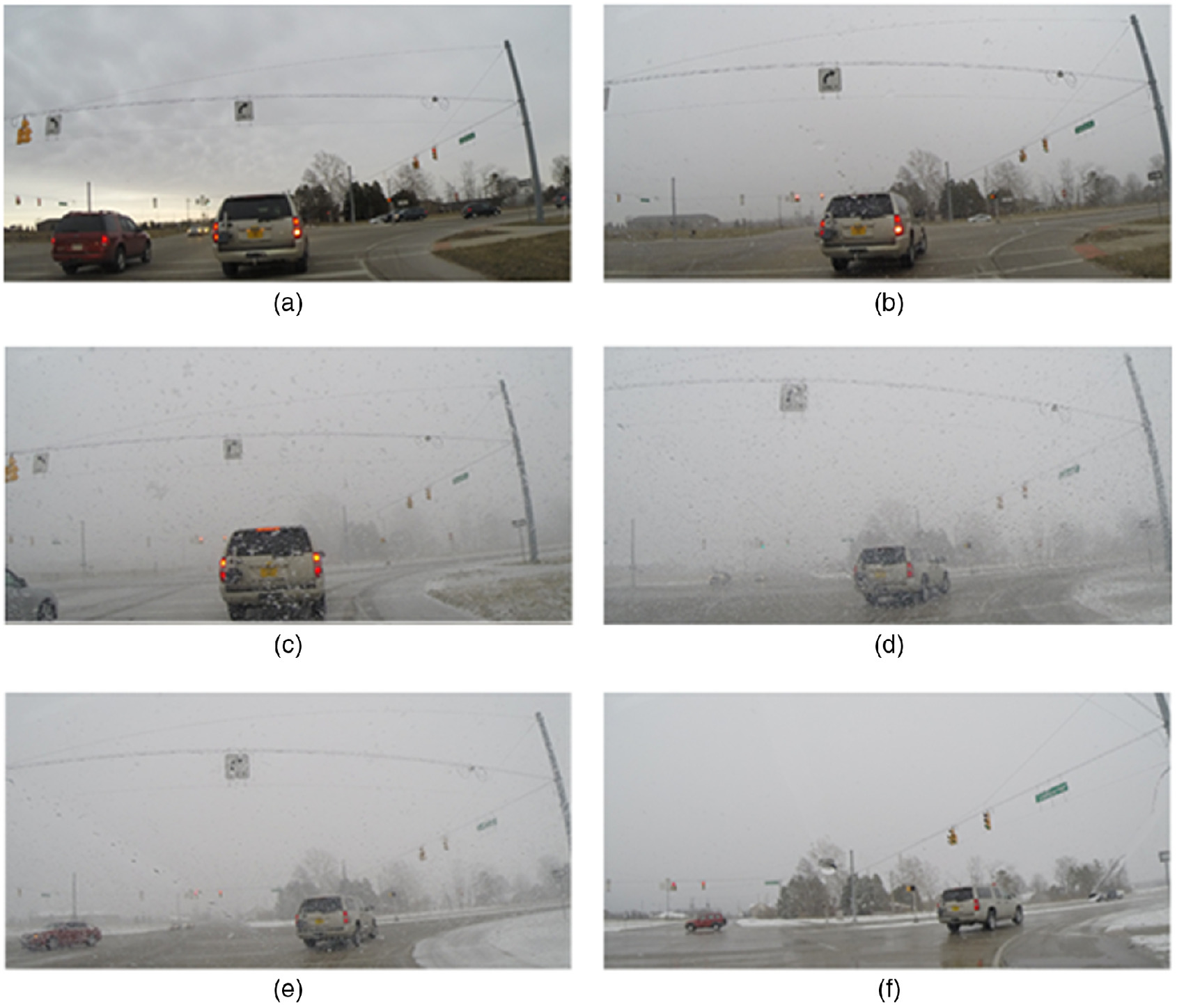
The callouts on Fig. 8 document the findings from 18 passes at Segment 34. In Fig. 8(a), Callout i indicates when the driver first noticed the road becoming wet [Fig. 9(b)]. However, the wet road did not impact the friction readings (Callout ii) but was reflected in the driver’s slight reduction in speed of about 1.6 to [Fig. 8(c), Callout iii]. The brake pressure applied during the fourth lap [Fig. 8(d), Callout iv] was not any less than the previous three laps. An important note is that the vehicle arrived at the intersection for the third lap indicated by Fig. 8(d), Callout v, where the vehicle did not come to a complete stop before making the turn. However, comparing the rate of change in brake pressure of the previous three laps with the fourth lap, there is a slight increase in the rate of application (positive pressure) of the brakes [Fig. 8(e), Callout vii].
By the sixth lap, the driver likely observed the link had started becoming snow-covered [Fig. 8(a), Callout viii]. The measured friction also started to drop [Fig. 8(b), Callout ix]. The top speed on the link also dropped about from top speeds recorded in the first three laps [Fig. 8(c), Callout x]. During this lap, the brake pressure applied remains high at its peak (Callout xi); however, the rate of change of brake pressure peaked at [Fig. 8(e), Callout xii], which was more than double of the first three laps. Fig. 9(c) shows the road condition during this period.
By the eighth lap, the friction had dropped to about 0.6 and the roadway was substantially covered with snow or slush [Fig. 9(d)]. The brake pressures start dropping below 15 bars at their peak [Fig. 8(d), Callout xiii] and the rate of brake pressure change also decreased in both the positive and negative directions [Fig. 8(e), Callout xiv].
By the 13th lap, the driver noticed the conditions improving slightly (Callout xv), and the friction was sustained above 0.7 briefly [Fig. 8(b), Callout xvi]. The road condition became more wet than snowy [Fig. 9(e)] and the driver started applying a greater amount of pressure [Fig. 9(d), Callout xvii]. The rate of change in brake pressure increased in both the positive and negative directions [Fig. 8(e), Callout xviii].
By the 17th lap, the road condition on the link had been rated consistently wet for a few laps by the driver [Fig. 8(a), Callout xix] and was reflected in the dashboard camera [Fig. 9(f)]. The friction value also approached 0.8 [Fig. 8(b), Callout xx], close to values reported on dry pavement. While the static brake pressures applied remained consistently higher during the high friction laps compared to the low friction laps, the rate of change of brake pressure by qualitative observation was not substantially different between laps of high and low friction [Fig. 8(e), Callout xxi]. The laps with the greatest variation in rate of change in brake pressure appeared to be during the shoulder periods where the conditions start deteriorating substantially or when the conditions start improving; however, it is difficult to identify clear trends from the time series representation of the data. This behavior is explored further using statistical methods in the next section.
Analysis
Braking Behavior by Speed
The static brake pressure and change of brake pressure data collected from icy conditions on February 11 and dry conditions from July 9 were compared using cumulative frequency distribution (CFD) diagrams. Data from the same driver and on the same circuit was collected for each day. Fig. 10 shows the CFDs for static brake pressure [Figs. 10(a–e)] and braking rate [Figs. 10(f–j)] with the data grouped into five speed categories. Braking data below were excluded from the analysis to filter out any arbitrary braking application, such as at a traffic signal when the vehicle was stationary.
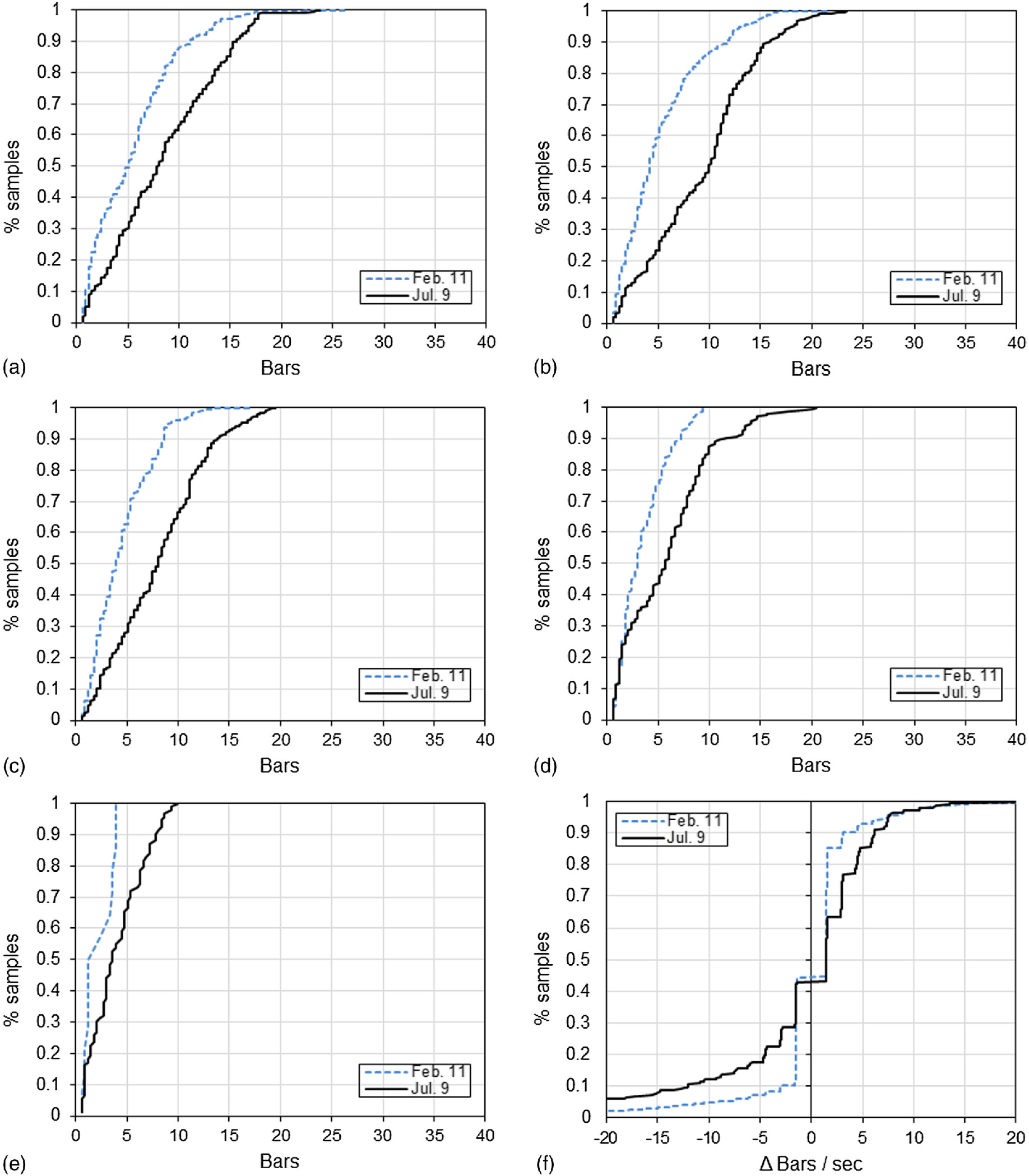
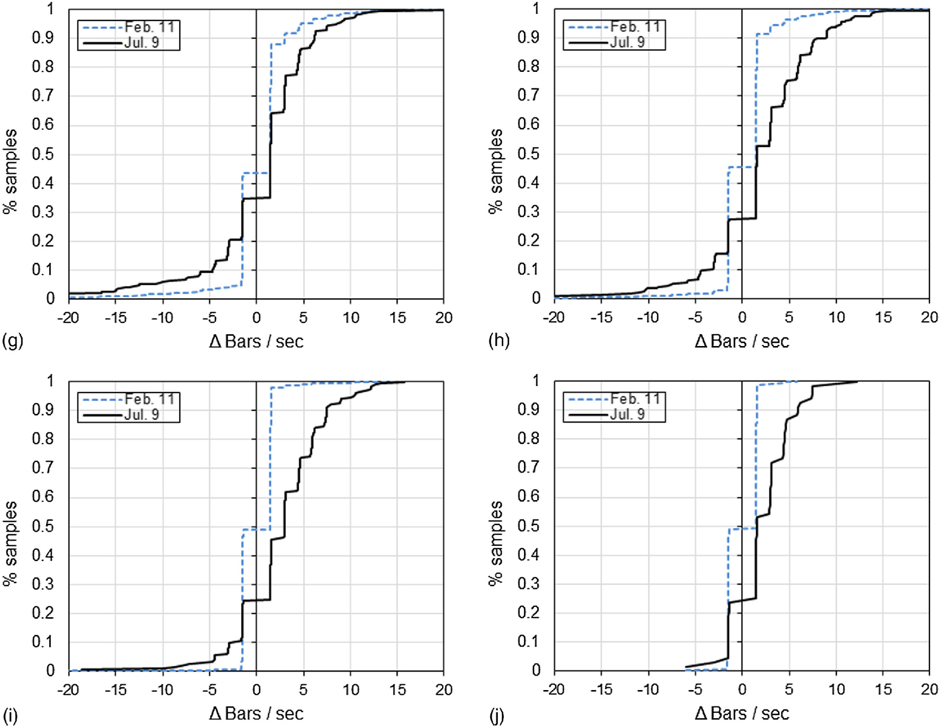
Figs. 10(a–e) shows that for all of the speed categories, the pressure applied was greater during the dry condition than the icy condition. At , the pressure was 3 bars greater at the median during the dry condition, and this doubles to 6 bars at , or about 60%. At , the difference was 5 bars at the median, but at and above , this difference decreases to about 2 bars. These figures suggest that at higher speeds and lower speeds, there tend to be smaller differences in braking application than when the vehicle was traveling at speeds between the two ranges. The speed range at which the greatest median difference in brake pressure applied between the dry and icy condition was from 16 to .
Figs. 10(f–j) shows the change of brake pressure during icy conditions was more conservative overall than during dry conditions. In the range of , the change of brake pressure applied was about faster at the 80th percentile than in icy conditions, and the change of brake pressure released was also about faster at the 20th percentile. In the range of , the change of brake pressure applied was similar to at at the 80th percentile, but the change of brake pressure released had almost no difference at the 20th percentile. In the range of , the difference in the change of brake pressure between the dry and icy conditions increased to at the 80th percentile. However, the change of brake pressure release in dry conditions continued to approach the rates at icy conditions at these higher speeds. At speeds from 48 to , the change of brake pressure applied continued to diverge from the dry conditions at the higher pressures; at the 80th percentile the change of brake pressure in icy conditions was only about , or 25% of the change of brake pressure in dry conditions. Braking pressures during the icy conditions did not reach over until well above 95th percentile of braking samples. At speeds over , the braking application rate in the dry conditions were slightly lower than at lower speeds. The data from these results suggest that the change of brake pressure applied at speeds between 32 and can be used as an indicator to differentiate road conditions based on user behavior.
Using a two-sample Kolmogorov-Smirnov (KS) test, there was found to be high significance () disproving the null hypothesis between the braking samples of the two dates at all speed categories.
Braking Behavior by Friction Level
To see if there was any correlation between the braking rate and the different friction levels experienced on the roadway, the samples were joined spatially and temporally and plotted against each other in Fig. 11. The graph in Fig. 11(a) shows data from the ice storm on February 11 while Fig. 11(b) shows data from the deteriorating winter storm condition on March 24. Because one driver was collecting data on February 11 and another for March 24 on different routes, there will be differences in braking behavior. Normalizing different drivers’ behavior across different routes, under different vehicle and equipment setups are subjects for many future research topics.
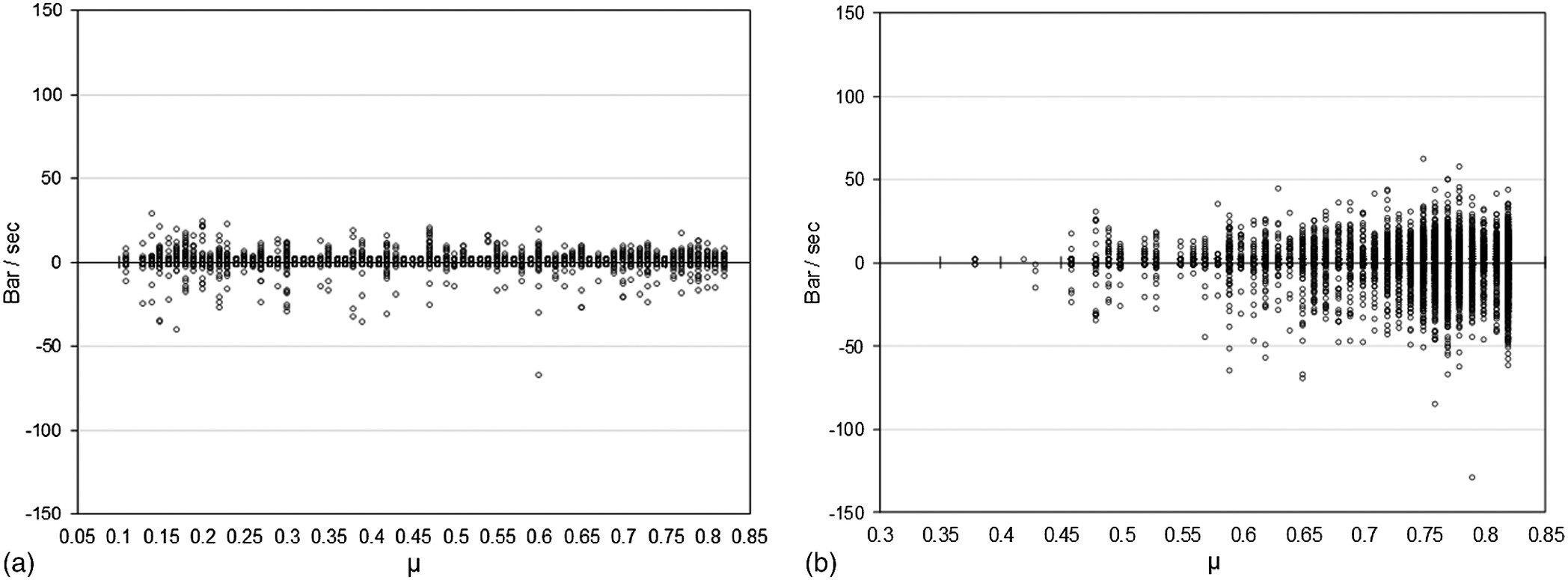
On February 11, the friction levels experienced were over a much wider range, from a value of 0.82 down to 0.11. The experiment also started in icy conditions with no reduction or improvement of friction conditions through the test period other than on different road segments on different parts of the loop. The range of braking rates were mostly within to and were pretty consistent throughout the range of friction values. There was a slight increase in the change of brake pressure application and release below of 0.2.
On March 24, the experiment started under dry conditions with high friction values () and within 2 h had deteriorated into snowy conditions with some areas experiencing . In Fig. 11(b), the graphs show the range of friction values for that day were sampled between and . The scatter plot of brake pressure rates follows a tapering conical shape—as the friction values decrease, the extremities of the change of brake pressure also appeared to be curtailed. This may be due to the driver adjusting his braking behavior as the conditions deteriorated throughout the day. Also, for the friction values in the range of –, there appears to be a noticeable decrease of the vertical bulge in the data, which may hint to the limit where the driver makes their adjustment to changing road conditions over the test period.
Significance of Braking Variance under Different Friction Levels
To verify whether the trends shown in Fig. 11(b) were significant, the Brown-Forsythe test (Brown and Forsythe 1974) for the equality of group variances was used to compare the rates of braking in each friction group. The test determines whether the variances of each group were equal based on each sample’s absolute difference from the group median. The change of brake pressure data from March 24 was divided into four groups using the floor value of the corresponding friction sample to the nearest . Friction values below were not included due to few samples from this day.
Table 3 shows the P-values of the test output for the 10 combinations of the four friction groups. At 95% confidence level, the variance of braking rates was found to be statistically significant between most friction groups except for , and . This suggests that in a scenario where road conditions deteriorated, the rate of change in brake pressure applied is different for different road conditions. However, the data does not suggest whether different drivers will respond accordingly in deteriorating road conditions.
| 0.5 | 0.6 | 0.7 | 0.8 | |
|---|---|---|---|---|
| 0.4 | 0.006 | 0.036 | ||
| 0.5 | — | 0.177 | 0.001 | 0.002 |
| 0.6 | — | — | ||
| 0.7 | — | — | — | 0.676 |
Results and Discussion
The high-frequency in-vehicle data collected for this study under inclement weather conditions suggested that extreme but rare events, such as large differentials of wheel angular velocity, traction control, and ABS intervention, were useful indicators for specific areas of the roadway where there were friction concerns. Because of their frequency of occurrence and pragmatic driver behavior to adjust to such conditions to prevent them, these events were not sufficient to approximate road conditions over a wide area. Moreover, at the local arterials level, because of stochastic variations of controlled stops such as from traffic signals and turning movements, speed may not be the best indicator of deteriorating conditions over a short time period.
The high-frequency braking data examined in this study over two winter storm events suggested that the change of brake pressure may be a useful early indicator of deteriorating road conditions based on the behavioral response of the driver to adjust to the perceived conditions. However, during conditions that were already slippery, the driver may be more careful from the beginning of the drive and not adjust the change of brake pressure too much. Therefore, it would be difficult to assess the conditions from the braking data alone. Fig. 12 shows a time-series plot of the sampled MARWIS friction values and the variance of the change of brake pressure from the March 24 experiment. Only braking data at speeds between 32 and were used, because from the analysis this range was found to have the greatest difference between inclement and noninclement conditions. The data samples were aggregated into 5-min values, taking the minimum friction value sampled and the average variance of the change of brake pressure during each of the 5 min. Callout i indicates the period before any substantial deterioration in conditions were detected; there was a slow ramp-up to around , which then hovered around this rate for 30 min. Callout ii shows the first instance where there was a relatively sharp jump in the variance and a subsequent steep drop within a 5-min period, compared with the previous 60 min. At this time, the minimum friction values obtained from the MARWIS were still excellent at 0.82. This indicates that the driver was perceiving the road conditions changing either due to falling snow or pavement condition and adjusting their braking behavior.
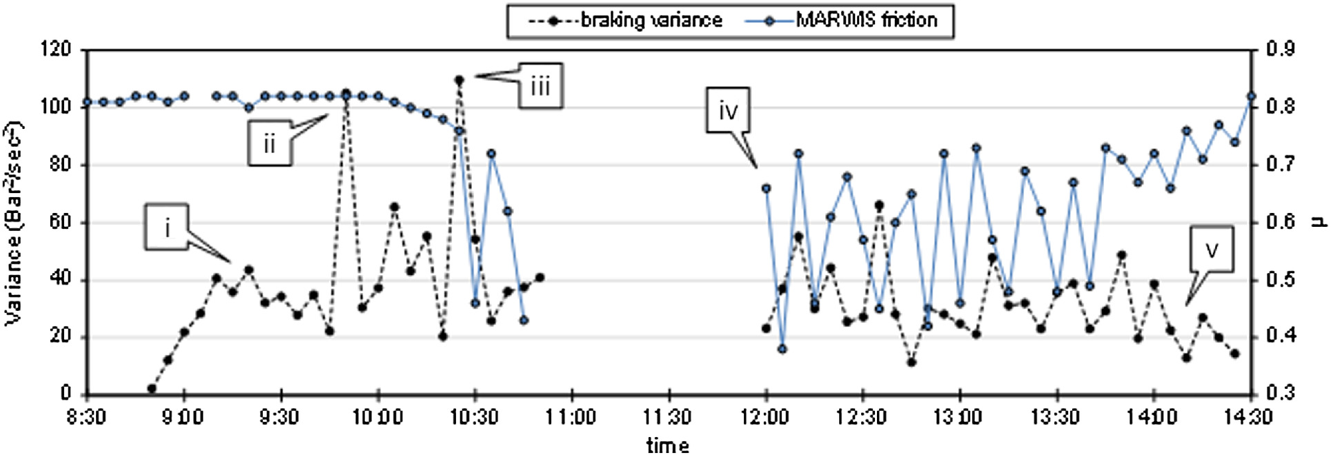
Callout iii shows another jump in the variance to a maximum of , but this time the corresponding minimum friction value also dropped to about , and then down to in the next 5 min. As the minimum friction values fluctuated during this time, the braking variance tapered off and did not show any sharp drops or increases past the initial two spikes at Callout i and ii. Later in the day (Callout iv), as the vehicle traveled between segments of roadway with higher and lower levels of friction, the braking variance showed fewer dramatic spikes compared to the morning, but still had some peaks between 40 and . Later in the afternoon, as the friction levels recovered, the variance also started to peak less, with minimums below . These observations suggest that the change of brake pressure can be used as a surrogate for the observed road condition at the leading edge of a winter storm and during the recovery period as conditions improve. However, these may not be reliable indicators during ongoing events where drivers are already accustomed to the winter conditions. Furthermore, the response behavior may be different for different drivers, so that a longer analysis period would be needed to characterize each driver’s driving style, and identify the thresholds at which nontypical driving conditions start occurring.
Conclusion and Future Work
The experiments conducted in this study demonstrated the application of high-frequency vehicle CAN data for observing winter weather road conditions. A system was deployed to collect wheel tick and brake pressure data at 100 to 200 ms time resolution. A web application was developed to display windshield wipers, hazard lights, traction control, and ABS activations for both real-time and historic events during an ice storm. Additionally, two separate winter events with independent road friction validation were used as test cases to demonstrate the applicability of using CAN data to monitor changing road conditions.
Key findings in this study suggest the following:
1.
A driver may reduce their applied braking pressure in deteriorating road conditions up to 60% at the median intensity;
2.
Braking pressures applied during wintry conditions were most different compared to dry conditions at speeds between 32 and where the heaviest braking was performed;
3.
The variance of the change of brake pressure was found to be significantly different during deteriorating road conditions;
4.
Wheel slip data alone may not account for adjustments to driving behavior that would mask actual slippery road conditions;
5.
Extreme vehicle intervention events such as traction control and ABS were typically rare, even at locations where very low friction values were measured; and
6.
Speed data alone may not be sufficient to characterize changing road conditions on arterials.
Finding 3 is particularly interesting. The driver anticipated deteriorating conditions at least 15 minutes before the road was actually slippery. This has potential for predicting deteriorating conditions ahead of time. Furthermore, it shows that images labeled by humans do not represent the ground truth friction. There is tremendous opportunity in the area of winter road research to leverage the in-vehicle data collection, processing and analysis methods presented in this study over a large fleet and a larger driver pool, and for different length journeys. For instance, different vehicles with front- or rear-wheel drivetrains and type of tires equipped may reveal slip conditions even more effectively. Having data over different equipment and demographic groups would validate or disprove using the data elements currently employed in this study and estimate the sample size needed to correctly identify changing road conditions. For example, some drivers may prefer to brake at the same rate even as conditions deteriorate.
Further tests may also suggest incorporating new data elements such as gas pedal usage, lateral acceleration, and air temperature sensors for determining road conditions. Moreover, applying these and similar methods in a real-time system with an informative interface, given enough protections to encrypt and secure anonymized user data, can be leveraged by agencies to operate and maintain their roads during winter events without costly infrastructure. These technologies can be further synergized with existing networks of automatic vehicle location (AVL) fleets such as snowplows.
Notation
The following symbols are used in this paper:
- static brake pressure (bars);
- wheel tick count integer;
- coefficient of friction; and
- angular velocity ().
Data Availability Statement
Some or all data, models, or code generated or used during the study are proprietary or confidential in nature and may only be provided with restrictions. Items include the following:
•
CAN data—wheel tick, brake pressure, speed, and location data can be provided with restrictions;
•
MARWIS data—no restrictions; and
•
Dashcam image data—no restrictions.
Acknowledgments
This work was supported by the Indiana Department of Transportation. A test vehicle for data collection, software, and hardware components were provided by the Volkswagen Electronics Research Lab for this study. HERE Global BV provided the API reading the geometry of road links for this research. Google Maps was used for the mapping interface in accordance with guidelines detailed at: https://www.google.com/permissions/geoguidelines/.
Disclaimer
The contents of this paper reflect the views of the authors, who are responsible for the facts and the accuracy of the data presented in this paper, and do not necessarily reflect the official views or policies of the sponsoring organizations. These contents do not constitute a standard, specification, or regulation.
References
Bray, E. T. 2014. “The Javascript object notation (JSON) data interchange format.” Accessed April 7, 2020. https://www.rfc-editor.org/info/rfc7159.
Brown, M. B., and A. B. Forsythe. 1974. “Robust tests for the equality of variances.” J. Am. Stat. Assoc. 69 (346): 364–367. https://doi.org/10.1080/01621459.1974.10482955.
Casselgren, J. 2018. RSI fas II—Road status information. Dynamisk väglagsinformation, AS II—Slutrapport, 154, Borlänge, Sweden: Trafikverket.
Cox, R. W. 1984. “Local area network technology applied to automotive electronic communications.” IEEE Trans. Ind. Electron. Control Instrum. 32 (4): 327–333. https://doi.org/10.1109/TIE.1985.350105.
FHWA (Federal Highway Administration). 2015. Road weather management performance measures survey, analysis, and report. Washington, DC: FHWA.
FHWA (Federal Highway Administration). 2017a. Regional assessment of weather impacts on freight. Washington, DC: FHWA.
FHWA (Federal Highway Administration). 2017b. Road weather management performance measures update. Washington, DC: FHWA.
FHWA (Federal Highway Administration). 2018. “How do weather events impact roads?” Accessed April 7, 2020. ops.fhwa.dot.gov/Weather/q1_roadimpact.htm.
Fielding, R. T. 1996. “Hypertext transfer protocol—HTTP/1.0.” Accessed April 7, 2020. https://www.rfc-editor.org/info/rfc1945.
Gerstenmeier, J., and W. Weber. 1987. “Traction control (ASR): An extension of the anti-lock braking system (ABS).” In Vol. 280 of Proc., 6th Int. Conf. on Automotive Electronics, 29–35. London: Institution of Electrical Engineers.
Hainen, A. M., S. M. Remias, T. M. Brennan, C. M. Day, and D. M. Bullock. 2012. “Probe vehicle data for characterizing road conditions associated with inclement weather to improve road maintenance decisions.” In Proc., IEEE Intelligent Vehicles Symp., 730. New York: IEEE.
Hartkopp, O. 2012. “The CAN networking subsystem of the Linux kernel.” In Proc., 13th Int. CAN Conf. (iCC). Nuremberg, Germany: CAN in Automation.
Hartley, J. 1974. “Anti-lock braking.” In Vol. 13 of Automotive design engineering. London: Design Engineering Publications.
Kiencke, U., S. Dais, and M. Litschel. 1986. “Automotive serial controller area network.” In Proc., SAE Technical Papers, International Congress and Exposition. Warrendale, PA: SAE International.
McMillin, R. J. 1984. “Communications, control, and display.” In Proc., Int. Congress on Transportation Electronics, 22–24. New York: IEEE.
Pisano, P., L. Goodwin, and M. Rossetti. 2008. “Highway crashes in adverse road adverse weather conditions.” In Proc., 88th Annual Meeting American Meteorological Society. Boston: American Meteorological Society.
Zhao, J., J. Zhang, and B. Zhu. 2014. “Development and verification of the tire/road friction estimation algorithm for antilock braking system.” In Mathematical problems in engineering. New York: Hindawi Publishing.
Information & Authors
Information
Published In

Journal of Transportation Engineering, Part A: Systems
Volume 146 • Issue 8 • August 2020
Copyright
This work is made available under the terms of the Creative Commons Attribution 4.0 International license, https://creativecommons.org/licenses/by/4.0/.
History
Received: Nov 30, 2018
Accepted: Jan 6, 2020
Published online: May 29, 2020
Published in print: Aug 1, 2020
Discussion open until: Oct 29, 2020
Authors
Metrics & Citations
Metrics
Citations
Download citation
If you have the appropriate software installed, you can download article citation data to the citation manager of your choice. Simply select your manager software from the list below and click Download.