Acceleration and Deceleration Calibration of Operating Speed Prediction Models for Two-Lane Mountain Highways
Publication: Journal of Transportation Engineering, Part A: Systems
Volume 143, Issue 7
Abstract
In this study, to calibrate the acceleration/deceleration rates in operating speed prediction models, driving tests were performed on two-lane mountain highways using passenger cars, and continuous longitudinal acceleration data were collected. The acceleration/deceleration rates of large vehicles such as coaches and heavy trucks were also measured from the roadside. The collected data were used to determine the cumulative frequency profiles and statistical distribution characteristics of the peak acceleration for different types of vehicles. Based on the established correlations, models of acceleration/deceleration versus road geometry features were developed. The key findings of this study are as follows: First, for passenger cars, the deceleration rate is obviously greater than the acceleration rate. Therefore, it would be inappropriate to use the same value for both the rates in speed prediction models. Instead, acceleration and deceleration should be calibrated separately. Second, none of the breakpoints on the acceleration/deceleration cumulative frequency curves appears at the 85th percentile; rather, they appear closer to the 95th percentile. Therefore, the common practice of using the 85th percentile in highway design should probably be reconsidered. Third, for large coaches, the acceleration and deceleration rates are quite similar, whereas for heavy trucks, the deceleration rate is significantly larger than the acceleration rate. The acceleration and deceleration rates of heavy trucks are both lower than those of coaches. Finally, for passenger cars driving around a curve, a negative correlation exists between the acceleration/deceleration rate and curve radius and a positive correlation exists between the acceleration/deceleration rate and deflection angle.
Introduction
Over the past two decades, design-consistency analysis methods based on operating speed profiles have become primary tools for road geometry safety evaluation because of their advantages of fast processing, high efficiency, and good user convenience. Such methods have played a critical role in limiting the frequency of accidents on mountain highways and reducing the formation of accident-prone highway sections. The function of operating speed prediction models is to predict a continuous-speed curve for vehicles driving along a road. In addition to the horizontal geometry, such models are also able to consider three-dimensional (3D) geometric effects. The rationality of the forms and coefficients of a model determines the accuracy of its speed prediction, which influences the reliability of the evaluation results used for ensuring design consistency in highway alignments. Therefore, improving existing operating-speed models and proposing new models are subjects of interest in the field of highway engineering.
A 3D road surface can be decomposed into horizontal, vertical, and cross-sectional components. The horizontal alignment can be further decomposed into straight, spiral, and circular components. Most existing models have been developed for a specific type of road section or single/multiple geometric elements. Operating speed models currently in use include horizontal curve models (Christopher and Mason 1995; Easa and Mehmood 2007; Jacob and Anjaneyulu 2013), straight road models (Luca et al. 2014), curved slope models (Gibreel et al. 2001; Xu et al. 2015), desired speed models (Crisman et al. 2005), roadside interference models (Fitzpatrick et al. 2005), traffic impact models (Shao et al. 2015), tunnel models (Fang et al. 2010), and interchange ramp models (Zhang et al. 2014).
Operating speed prediction models proposed roughly over the last 30 years by researchers from the United States (U.S.), Canada, and some European countries listed in Table 1, along with the independent variables (predictors) used in the model. As seen in the table, , CCR, , and are the most commonly used predictors irrespective of the location (United States, Canada, or Europe). However, factors such as the terrain conditions, road characteristics, traffic composition, and automobile performance may differ for different countries and regions; therefore, the road geometry features (i.e., the meaning of variables) that have a major impact on the operating speed can have significant differences, which is represented as follows. First, in the United States and Canada, researchers often use the predictor to establish the model, whereas in Europe, this predictor is not used. Second, in addition to the predictors and CCR, the operating speed model for a horizontal curve in Europe usually contains (operating speed on the approach tangent of the curve) or (speed at curve entry). In contrast, these two predictors are not employed in the models from the United States and Canada probably because the terrain in North America is flatter than that in Europe; therefore, in North America, the ratio of the curve length to the total road length is smaller, and the average spacing between adjacent bends is larger. However, in mountainous European countries such as Italy and Spain, two-lane highways generally have intensive horizontal curves, and hence, the operating speed on a bend is greatly impacted by the presence of an adjacent bend. In addition, the structure of operating speed models from Italy and Spain is more complex (e.g., Montella et al. 2014; Castro et al. 2011; Camacho-Torregrosa et al. 2013). Note that the models proposed by Donnell et al. (2001) from the United States and Gibreel et al. (2001) from Canada have more predictors, but that is because the former model is intended for heavy vehicles, whereas the latter model is intended for 3D highway alignment. To understand what the notations in Table 1 indicate, refer to the Appendix at the end of this paper.
| Literature reference | Country | Model | Predictors |
|---|---|---|---|
| Glennon et al. (1986) | U.S. | ||
| Lamm and Choueiri (1987) | U.S. | CCR, , , | |
| Ottesen and Krammes (1994) | U.S. | CCR, | |
| Islam and Seneviratne (1994) | U.S. | ||
| Krammes (1995) | U.S. | , , | |
| Voigt (1996) | U.S. | ||
| Pasetti and Fambro (1999) | U.S. | ||
| Fitzpatrick (2000) | U.S. | , | |
| , , | |||
| , | |||
| Ottesen and Krammes (2000) | U.S. | , | |
| McFadden and Elefteriadou (2000) | U.S. | , , | |
| Donnell et al. (2001) | U.S. | , , , , | |
| Morrall and Talarico (1994) | Canada | ||
| Transportation Association of Canada (TAC) (1999) | Canada | , | |
| Gibreel et al. (2001) | Canada | , , , , , , , , | |
| Misaghi and Hassan (2005) | Canada | ||
| Nie and Hassan (2007) | Canada | CCR | |
| Castro et al. (2008) | Spain | ||
| Castro et al. (2011) | Spain | , | , , |
| , | |||
| , | |||
| Camacho-Torregrosa et al. (2013) | Spain | , , | |
| , , | |||
| Kerman et al. (1982) | U.K. | , | |
| Guidelines for the design of roads (1984) | Germany | CCR, | |
| Lamm et al. (1995) | Germany | CCR | |
| Setra (1986) | France | CCR | |
| Cardoso et al. (1998) | Portugal | , | |
| Kanellaidis et al. (1990) | Greece | ||
| Lamm et al. (1995) | Greece | CCR | |
| Crisman et al. (2005) | Italy | , | |
| CCR, | |||
| Dell’Acqua et al. (2007) | Italy | , | |
| , | |||
| Luca et al. (2014) | Italy | , CCR, RES, INT, | |
| , , INT, | |||
| Montella et al. (2014) | Italy | , , CCR | |
| , CCR, , , | |||
| , , CCR, | |||
| , , , CCR |
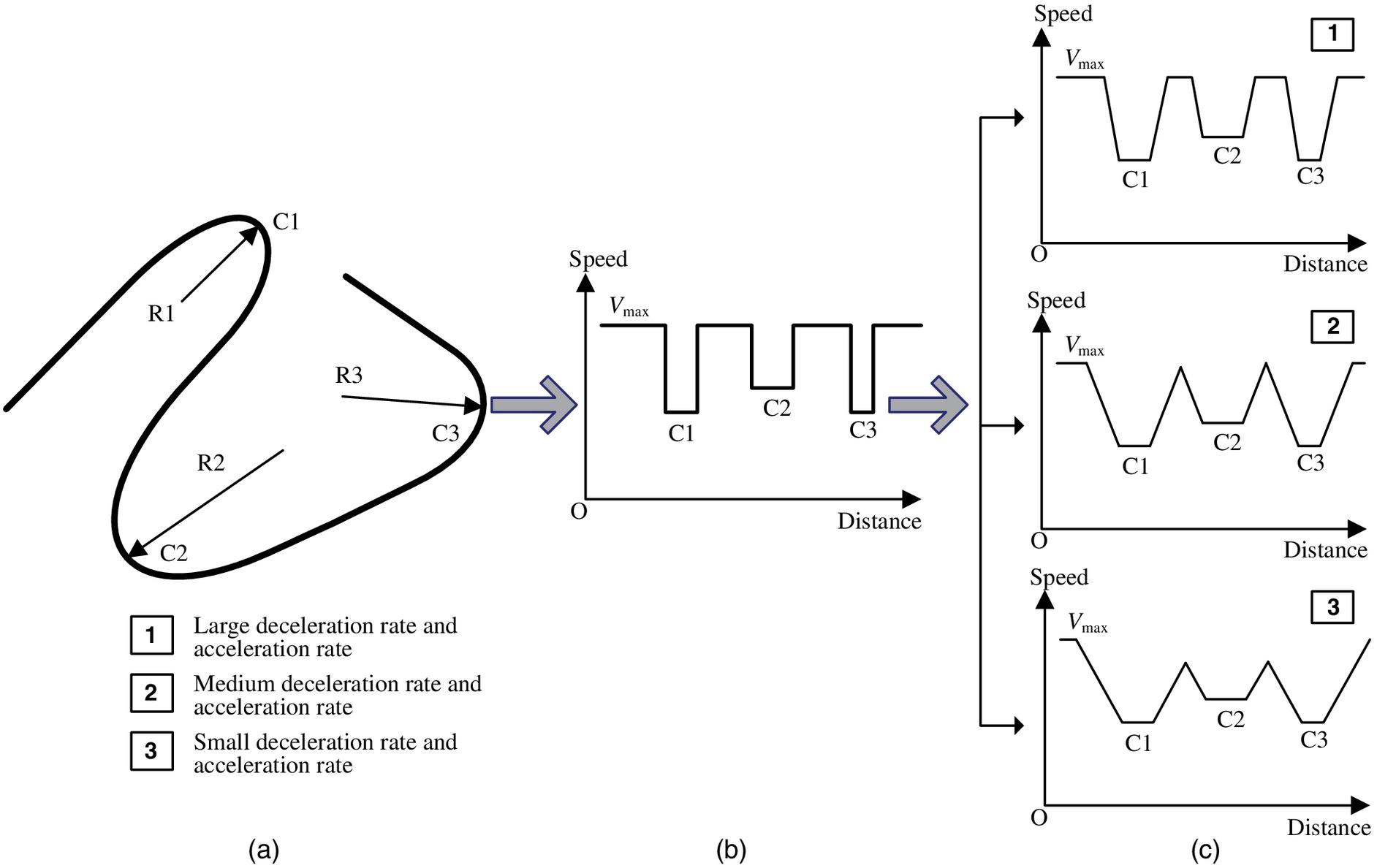
The operating speed varies on a road depending on two factors: the speed on different types of road segments (such as circular section or tangent), and speed adjustments made when transitioning between adjacent road segments. An example of the second factor is the deceleration made while entering a curve and the acceleration provided while exiting a curve; hence, this factor can be described in terms of vehicular acceleration/deceleration. As Fig. 1 shows, for a given road section, the operating speed profiles will have different shapes for different acceleration/deceleration rates. Extensive research has been conducted on this subject in China and other countries. In several of these studies, the acceleration and deceleration rates are both assumed to be equal to (Lamm et al. 1988) or (Echaveguren and Basualto 2003; Laurel and Tarek 2011). In other studies, they are both assumed to be within a certain range [, ], and it is common practice to employ linear interpolation within this range based on the current operating speed, which usually yields a smaller acceleration at a higher speed (Liu et al. 2010). Another hypothesis assumes constant acceleration/deceleration between two adjacent road elements, with the magnitude of the acceleration/deceleration determined by the difference in speeds on the two adjacent elements and the distance between them (Montella et al. 2014; Hashim et al. 2016). Researchers have also used experimental data to model the acceleration rate–speed relationship (Moon and Yi 2008) and acceleration rate–acceleration distance relationship (Gao et al. 2004). However, because these models do not differentiate between acceleration and deceleration, they are unable to capture the significant differences in the magnitudes of acceleration and deceleration caused by differences in the dynamic properties of vehicles (Fitzpatrick 2000; Camacho-Torregrosa et al. 2013; Montella et al. 2014). Thus, the results are not likely to accurately reflect actual vehicle operating characteristics.
In some studies, acceleration/deceleration rate–curve radius models have been constructed based on small-scale experimental data (Shao et al. 2011; Fitzpatrick 2000). However, because of the limited number of road samples considered, these models are restricted in their range of applicability. Other studies have considered acceleration/deceleration distribution characteristics based on observed speed or acceleration data. For instance, Altamira et al. (2014) used vehicle acceleration/deceleration data on horizontal curves and curved slopes to derive a relationship between the acceleration/deceleration rate and the distance to a curve entry/exit. Tokunaga et al. (2005) used a small passenger car driven on mountain roads to collect continuous acceleration/deceleration data, which were analyzed to assess the effects of day and night, summer and winter, and the use of electronic navigation devices on driver behavior. Based on speed measurements of vehicles on different cross sections and the distances between adjacent cross sections, Perco and Robba (2012) determined the distribution characteristics of acceleration and deceleration of vehicles on curved road segments.
As described above, previous research on automobile acceleration/deceleration suffers from the following limitations. First, many of the assumptions made in the previous studies were not based on actual driving behavior. Instead, they were made primarily to simplify calculations, and thus, the predicted speed could be significantly different from real-world driving. Second, although some researchers have developed acceleration/deceleration regression models, the sizes of the sample datasets used were relatively small, which limits the applicability of these models to other roads until their reliability and appropriateness can be improved. Third, almost all previous research on this subject has been limited to observing small passenger cars; little research has been conducted on the acceleration/deceleration characteristics of heavy trucks or large coaches on mountain highways, particularly on two-lane mountain highways. In this study, acceleration data were collected from both natural driving tests (onboard tests) and roadside observation tests for characterizing the statistical distributions of the acceleration/deceleration of small passenger cars, heavy trucks, and coaches. Models relating acceleration/deceleration to road geometry elements were constructed for these different types of vehicles. The results obtained provide a means for calibrating acceleration/deceleration rates in operating speed models for mountain highways, thereby remedying the shortcomings of the existing models presented in the literature.
Methods
Tested Highways
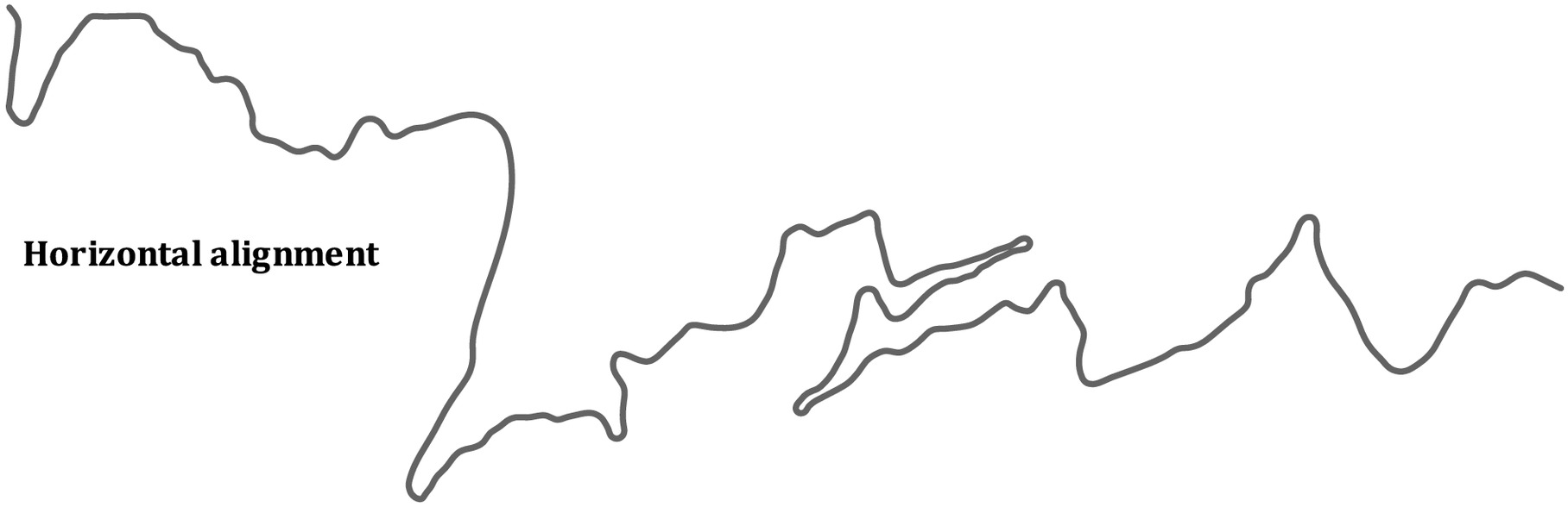
In mountainous regions, especially in middle and higher mountain areas, most of the public roads are two-lane highways. In this study, experiments were performed on six two-lane mountain highways in Chongqing, China (Table 2); in the table, represents the minimum radius used for horizontal curves. All these two-lane highways trace complex paths through rugged mountainous terrain. In each case, the roadside conditions were dangerous, and the accident/fatality rate was high. Fig. 2 shows a one-dimensional projection of a short section of Highway S102 between Wuxi and Yunyang.
| Road name | Design speed () | (m) | Measured length (km) | Terrain | Slope range (%) |
|---|---|---|---|---|---|
| S102 Wuxi–Yunyang section | 20–40 | 15 | 108.7 | Mountain | 3–10 |
| G212 Beibei–Hechuan section | 30 | 30 | 26.8 | Mountain | 2–8 |
| G319 Qianjiang–Xiushan section | 30–60 | 30 | 90.2 | Mountain | 2–7 |
| S103 Wanzhou–Fengjie section | 20–40 | 15 | 121.9 | Mountain | 3–9 |
| S201 Fengjie–Wuxi section | 20–40 | 20 | 74.8 | Mountain | 3–9 |
| S205 Dazu–Tongnan section | 40–60 | 60 | 45.2 | Mountain | 3–10 |
Test Vehicles and Drivers
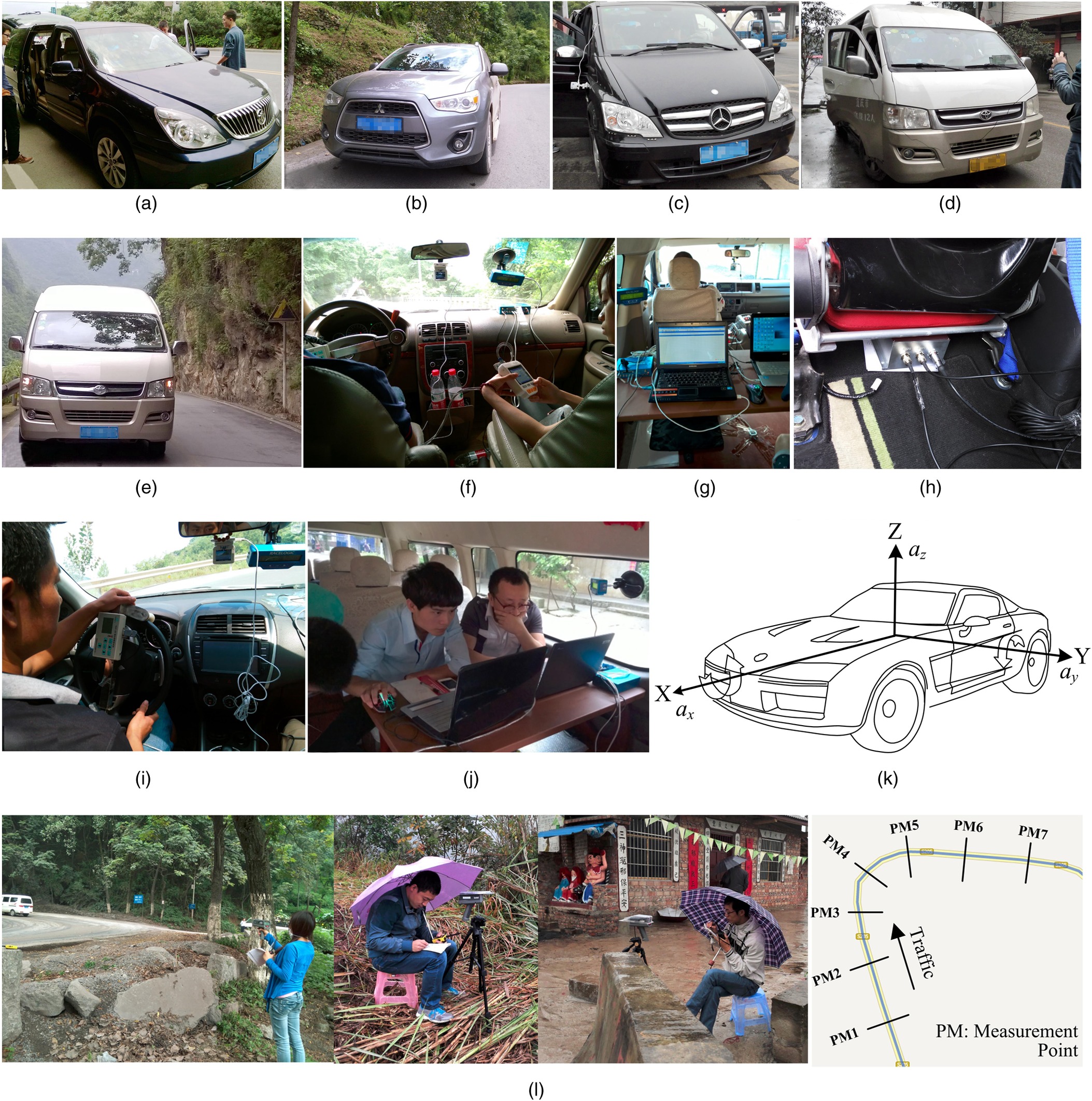
The vehicles used for onboard testing were a Mitsubishi ASX (2013 model, 2.0 L, automatic four-wheel drive, four seats), a Buick GL8 (2.4 L, business exclusive model, seven seats), a Toyota HIACE (2.7 L, standard manual model, nine seats), a modified Toyota HIACE (2.7 L, modified manual model, seven seats), and a Mercedes-Benz Vito (2011 model, 2.5 L, business model, seven seats), as shown in Figs. 3(a–e). Twenty-seven skilled drivers participated in the tests. Data from 23 of these drivers were used in the analyses that produced the final results. The 23 contributing drivers had driving experience ranging from 2 to 31 years, with an average of 12.9 years. Their ages ranged from 22 to 59 years, with an average of 38.2 years. Three or four drivers were assigned to each section of the tested road. Each driver made one round trip through a test section.
Experimental Methods
The acceleration/deceleration data were obtained from two sources. The first source was continuous road driving tests performed using onboard testing technology. The test drivers were instructed to drive their vehicles naturally (maintaining their normal driving habits), whereas the operating parameters of the vehicles, including the trajectory, speed, acceleration, and attitude, and visual data from the surroundings were collected continuously along the test routes, as shown in Figs. 3(f–j). This data collection method was employed primarily for small passenger cars. The trajectories were collected using a differential global positioning system (DGPS) with a centimeter-level accuracy. Continuous speed data were obtained by differentiating the planar DGPS output coordinates. Data on the surrounding environment were obtained using three 5-megapixel video cameras: one pointed straight ahead, one pointed to the right, and one pointed backward. Acceleration and attitude data were collected using an LP-RESEARCH Motion Sensor (LPMS, including a tri-axle gyroscope, tri-axle accelerometer, and tri-axle earth magnetic sensor), which is a micromechanical attitude and heading reference system. The data output from the LPMS included the time, longitudinal acceleration, lateral acceleration, vertical acceleration, roll angle, pitch angle, yaw angle, and some other parameters. The relationship between the direction of the tri-axle and local coordinate systems of the driving vehicle are described in Fig. 3(k). In this study, only the signal for the longitudinal acceleration was analyzed, with its positive and negative values indicating forward acceleration and braking deceleration, respectively.
The second source of data was off-road observations [Fig. 3(l)]. First, a section of the road was chosen. This section was then divided into smaller segments, with measurement points established on each characteristic cross section. Test personnel then used a radar velocimeter to record the speeds of the vehicles as they passed by. The large vehicles were identified by type, and two of these—large coaches and heavy trucks—were selected as the test objects. As a vehicle passed the first measurement point, the test personnel there used a portable two-way radio to report the vehicle type and features to the test personnel at the subsequent measurement points. The remaining test personnel assigned a number to this vehicle and recorded its speed. This guaranteed correspondence and consistency of the speed data for a given vehicle at different points. The combined data were recorded in the form , where = number of measurement points and = observed speed of a certain vehicle at measurement point . For the curves with short lengths, five observation points were set: one at the middle of the curve, one each at the curve entrance and exit, and one each on the preceding and succeeding tangents. In this way, four acceleration values were obtained. For longer bends, seven observation points were set, and accordingly, six acceleration values were obtained: (1) for continuous curves, the first point was located at the middle of the analyzed and preceding curves, and the last point was set at the middle of the analyzed and succeeding curve; and (2) for bends having long preceding/succeeding tangents, the first and last observation points were located on the tangents at a distance of 120–150 m from the entry/exit points of the analyzed curve.
The following formula was used to determine the average acceleration/deceleration rate between adjacent measurement points and :where = distance between measurement points and . The acceleration rate was defined as the positive with the largest magnitude, and the deceleration rate was defined as the negative with the largest magnitude. It is noted that this method was utilized to collect data for large vehicles. This method can be used to obtain observation data for more models (or axis numbers) because in China, there are more than 100 truck manufacturers, with the number of mainstream manufacturers alone being more than 10; therefore, trucks are available in numerous combinations of models and styles. Furthermore, different models may have significant differences in terms of dynamic performance; the manufacturing quality of different brands will be different even under the same loading conditions, and the operating condition of different vehicles will vary greatly.
(1)
It is important to note that different methods used to collect the axial acceleration data for the two types of vehicles (large vehicles and small passenger cars) may produce different magnitudes of deviations between the measured data and real values. For passenger cars, the LPMS system recorded data continuously at a sampling rate of 10 Hz. As a result, at least 100 data points were obtained for each horizontal curve (the travel time for a vehicle to pass by a horizontal curve was usually more than 10 s). The acceleration rates for large vehicles were calculated using only seven off-road measured values. For example, for the acceleration rates of vehicles leaving a curve, the data for the passenger cars had greater sample densities and were better able to capture the peak acceleration. In contrast, the acceleration data for the large vehicles represented the average acceleration between two relatively widely spaced measurement points, and this average value was smaller than the peak acceleration value between the two points.
Acceleration/Deceleration Distribution Characteristics for Passenger Cars
In many operating speed models, acceleration/deceleration is simplified as a constant, and it is common practice in Europe and North America to set this value to for passenger cars on two-lane highways. China’s Highway Safety Audit Guidelines (JTG/TB05-2015) suggest ranges for passenger cars () and large cargo vehicles () and assume that the acceleration and deceleration characteristics are the same. The highway capacity manual (HCM 2010) recommends a rate of () for both acceleration and deceleration if these rates are unknown for straight urban roads; for right turns, it recommends an acceleration rate of and a deceleration rate of . In Sweden, acceleration and deceleration rates are prescribed as in Swiss Norm 640 080b (Vereingung Schweizerischer Strassenfachleute 1992) to estimate the speed profile on the tangents between curves. In a report published by the U.S. Federal Highway Administration (1995, Report No. FHWA-RD-94-034), deceleration and acceleration are assumed to occur on the tangents approaching and leaving the curve, and both are set to , which is slightly greater than the rate for Sweden (Krammes 1995). In the present study, the authors examined these approaches to characterize acceleration and assessed their applicability to mountain highway conditions, vehicle performance, and driver behavior on two-lane mountain highways.
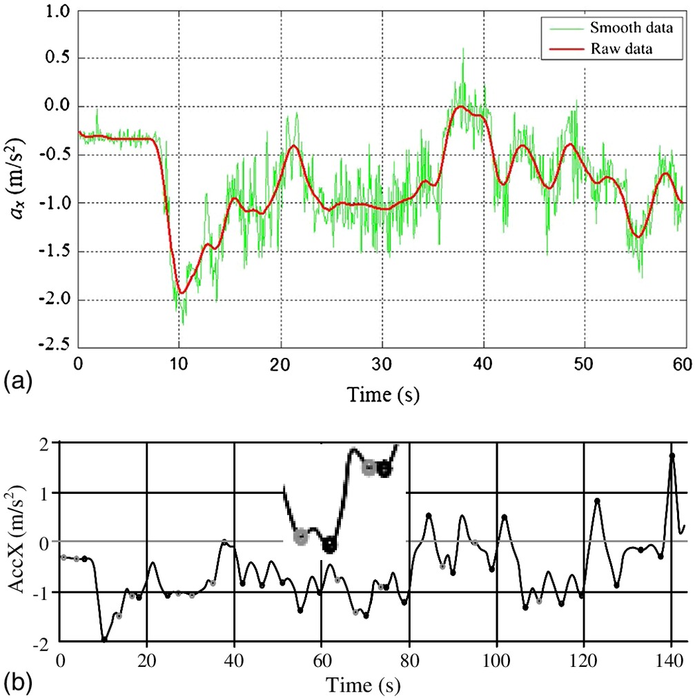
The continuous curves of longitudinal acceleration obtained from the LPMS units mounted in the test vehicles were processed. The data were filtered and smoothed to remove signal noise and glitches, as shown in Fig. 4(a). A peak extraction algorithm was then designed to determine the maximum deceleration and acceleration as each vehicle entered and exited each horizontal curve, as illustrated in Fig. 4(b). Next, the acceleration and deceleration peaks were collected separately and sequenced to obtain and , where and = peak acceleration and peak deceleration, respectively, and and = number of peak acceleration and deceleration values, respectively. Finally, the cumulative frequency curves of acceleration and deceleration were developed for each type of vehicle.
The measured results of the longitudinal acceleration for three drivers on the test road—National Highway G212—are presented in Figs. 5(a–i), where is the sample size of the measured data. The results in Figs. 5(a–c) represent the distribution of longitudinal acceleration versus the driving speed, cumulative frequency curves of longitudinal acceleration, and cumulative frequency curves of acceleration and deceleration, respectively, for the first driver; the speed considered here is the initial velocity when drivers are decelerating/accelerating their vehicles. From the scatter plot in Fig. 5(a), one can see that deceleration and acceleration have two different sets of variation characteristics with an increase in the driving speed. The amplitude of acceleration decreases as the initial speed increases; in contrast, a larger deceleration rate often corresponds to a higher initial speed. Data analysis indicates that during acceleration, the vehicle dynamic performance plays a major role; that is, the reserve accelerating ability is smaller at a higher speed, which results in weak acceleration. With regard to deceleration, the distribution characteristics are determined by the actual demand while driving on curvy roads because a higher speed at curve entry will require a larger reduction in the driving speed to ensure safe bend negotiation; consequently, the driver will have to adopt a large deceleration. The distribution of longitudinal acceleration versus the initial speed for the second and third drivers is presented in Figs. 5(d and e). The results for all the three drivers are shown in Fig. 5(f); they all exhibit similar variations with the initial speed, as illustrated in Fig. 5(j).
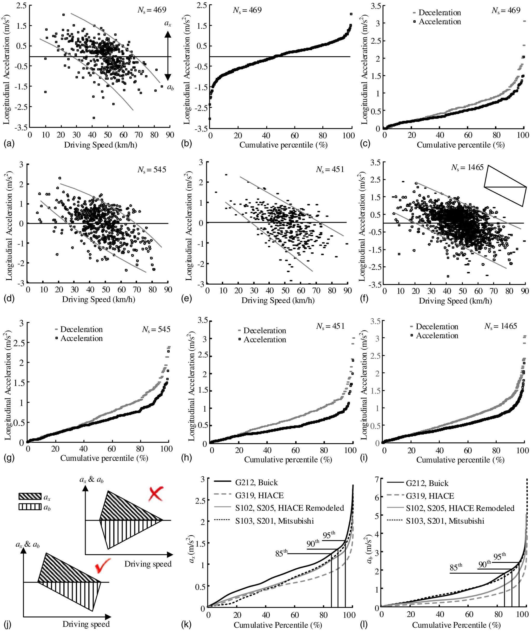
Figs. 5(g and h) show the cumulative frequency curves of and versus the initial speed of the second and third drivers. As in the case of the first driver [Fig. 5(c)], one finds that the deceleration is larger than the acceleration for the second and third drivers; and the difference between deceleration and acceleration is significant. Moreover, the personal characteristics of drivers can cause variations in the shape of the cumulative frequency curves. The results for all the three drivers on the G212 are shown in Fig. 5(i). The results for the other test roads are not described here owing to the limitation on the paper length.
Figs. 5(k and l) show the cumulative frequency curves of acceleration and deceleration for each type of vehicle. The 85th, 90th, and 95th percentile characteristic values are also indicated. Several obvious features are seen in the figures. First, the deceleration is greater than the acceleration, and the maximum deceleration rate is approximately twice the maximum acceleration rate. The reason for this difference is that the deceleration rate produced by braking depends on the friction coefficient of the pavement, . Thus, the deceleration rate can approach or even reach . On the other hand, as long as the pavement is in reasonably good condition, a vehicle’s acceleration depends on the torque of the engine and transmission/drive mechanisms. Considering current passenger car technology, the acceleration rate will obviously be less than the deceleration rate. Therefore, existing research findings and design specifications that do not address acceleration and deceleration separately are apparently not reasonable.
Second, the breakpoints of the cumulative frequency curves do not appear at the 85th percentile, as previously assumed. Instead, they are actually very close to the 95th percentile. This discrepancy is crucial, considering the fact that the core philosophy of the current road design methods concerning the operating speed is to base the design of road geometry features on driving behavior at the 85th percentile (breakpoint). The results of this research suggest that the 85th percentile philosophy needs to be corrected.
Third, differences exist between the acceleration and deceleration rates for different types of vehicles. Comparing Figs. 5(k and l), it is apparent that vehicles that exhibit high acceleration rates also exhibit high deceleration rates. However, an examination of the acceleration data only indicates that the 85th-percentile acceleration rates are greater than for all vehicles, except for the high-seating-capacity Toyota HIACE, which has a relatively low specific power. The 85th-percentile decelerations are even higher. Therefore, the adoption of a value of for both acceleration and deceleration is clearly inconsistent with actual driver behavior on two-lane mountain highways.
Table 3 lists the maximum and average acceleration and deceleration rates along with the 50th, 85th, 90th, and 95th percentiles extracted from the cumulative frequency curves. It is noticed that the 85th-percentile acceleration and deceleration rates, in particular, are 1.051 and , respectively, for all test vehicles. The characteristic percentile values can be used to calibrate the acceleration and deceleration rates in operating-speed prediction models for passenger cars on mountain highways. In the calibration, suitable adjustments can be made depending on the road conditions and vehicle types. The maximum values from the table can be used to establish boundary conditions for driving simulations.
| Test number | Acceleration () | Deceleration () | ||||||||||
|---|---|---|---|---|---|---|---|---|---|---|---|---|
| Maximum | Average | 50th | 85th | 90th | 95th | Maximum | Average | 50th | 85th | 90th | 95th | |
| I | 2.850 | 0.774 | 0.742 | 1.233 | 1.337 | 1.571 | 4.745 | 0.943 | 0.722 | 1.828 | 2.084 | 2.481 |
| II | 2.094 | 0.489 | 0.478 | 0.795 | 0.894 | 1.030 | 3.827 | 0.428 | 0.280 | 0.800 | 0.988 | 1.327 |
| III | 2.562 | 0.617 | 0.544 | 1.083 | 1.212 | 1.350 | 5.191 | 0.643 | 0.419 | 1.219 | 1.491 | 1.934 |
| IV | 2.818 | 0.611 | 0.598 | 1.138 | 1.266 | 1.475 | 7.132 | 0.913 | 0.764 | 1.619 | 1.917 | 2.355 |
| V (all vehicles) | 2.850 | 0.597 | 0.495 | 1.051 | 1.190 | 1.362 | 7.132 | 0.713 | 0.535 | 1.357 | 1.636 | 2.111 |
Note: I: G212 Beibei–Hechuan section, Buick GL8; II: G319 Qianjiang–Xiushan section, Toyota HIACE; III: S102 Wuxi–Yunyang section and S205 Dazu–Tongnan section, Toyota HIACE remodeled; IV: S103 Wanzhou–Fengjie section and S201 Fengjie–Wuxi section, Mitsubishi ASX; V: for all test vehicles.
Acceleration/Deceleration Distribution Characteristics for Large Vehicles
The operating speed models that have been proposed by researchers in Europe, North America, and Australia have been developed primarily for passenger cars (Misaghi and Hassan 2005; Abbas et al. 2011; Castro et al. 2011). The reasons for this are that passenger cars have higher speeds and have a greater effect on the design of horizontal alignments. However, in recent years, the transportation safety situation in China has been quite grim, with large-vehicle accidents, especially ones causing multiple deaths/casualties, becoming the most serious threat to road users. Hence, there is a pressing need for developing large-vehicle operating speed models to assess the suitability of roadway geometric designs for large vehicles.
Fig. 6 summarizes the longitudinal acceleration measurements obtained from off-road observations for large cargo vehicles (trucks weighing 20 t or more) on two-lane highways. In the figure, is the sample size of measured data. Positive values represent acceleration, and negative values represent deceleration. The scatter plot in Fig. 6(a) reveals a negative correlation between longitudinal acceleration and the driving speed. Fig. 6(b) shows the cumulative frequency curve for longitudinal acceleration. Taking the absolute values of the deceleration points and superimposing them on the acceleration points yields Fig. 6(c), and this figure shows that for heavy trucks, the deceleration values are clearly higher than the acceleration values.
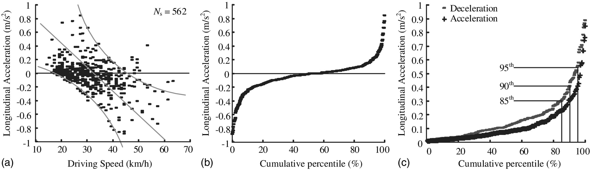
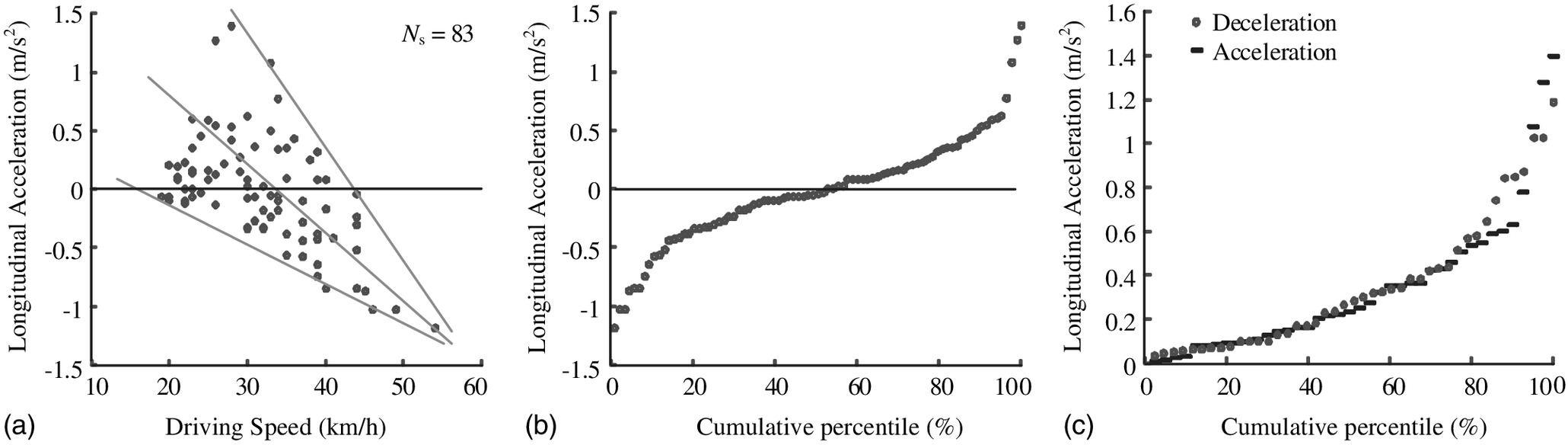
Fig. 7 summarizes the longitudinal acceleration results for large coaches (37 seats or more) obtained using the same method as that used for heavy trucks. Note that the acceleration data collection tasks for both trucks and coaches were carried out simultaneously on the same sections of the test roads; in terms of total traffic volume, the percentage of coaches is smaller than that of trucks, and therefore, the number of coaches that passed though the observation stations was less than the number of trucks. Two special features should be noted. First, the acceleration and deceleration rates for large coaches are at least 50% higher than those for heavy trucks. Large coaches carry lighter loads than heavy trucks and have higher specific powers per unit mass, so their performance is better in terms of acceleration and braking. Second, the difference between the acceleration and deceleration values is negligible. Therefore, for this type of vehicle, the same value can be used to calibrate both acceleration and deceleration in operating-speed models. Table 4 presents the maximum, average, and characteristic values for these two types of vehicles. These values can be used to calibrate the acceleration/deceleration rates in operating speed models for large vehicles on mountain highways and to establish boundary conditions for large-vehicle driving simulations.
| Vehicle type | Acceleration () | Deceleration () | ||||||||||
|---|---|---|---|---|---|---|---|---|---|---|---|---|
| Maximum | Average | 50th | 85th | 90th | 95th | Maximum | Average | 50th | 85th | 90th | 95th | |
| Coach | 1.396 | 0.342 | 0.230 | 0.584 | 0.627 | 1.075 | 1.187 | 0.354 | 0.280 | 0.690 | 0.845 | 1.026 |
| Cargo | 0.847 | 0.127 | 0.075 | 0.231 | 0.309 | 0.408 | 0.888 | 0.172 | 0.112 | 0.303 | 0.407 | 0.548 |
Relationships between Acceleration/Deceleration and Road Geometry Features
The main motivation for drivers to adjust their speeds on mountain highways is to adapt to the constantly changing horizontal curvature of the roadway. They tend to remain comfortably within the critical safe speed limit for horizontal curves, especially sharp curves with small radii. Fig. 8 shows the speed and acceleration of a passenger car as it traverses a short, complex section of Highway S102 between Wuxi and Yunyang. It is observed that every curve of the road causes a change in speed and hence a change in the longitudinal acceleration. This suggests that there may be a close correlation between the longitudinal acceleration and the geometric parameters of horizontal curves.
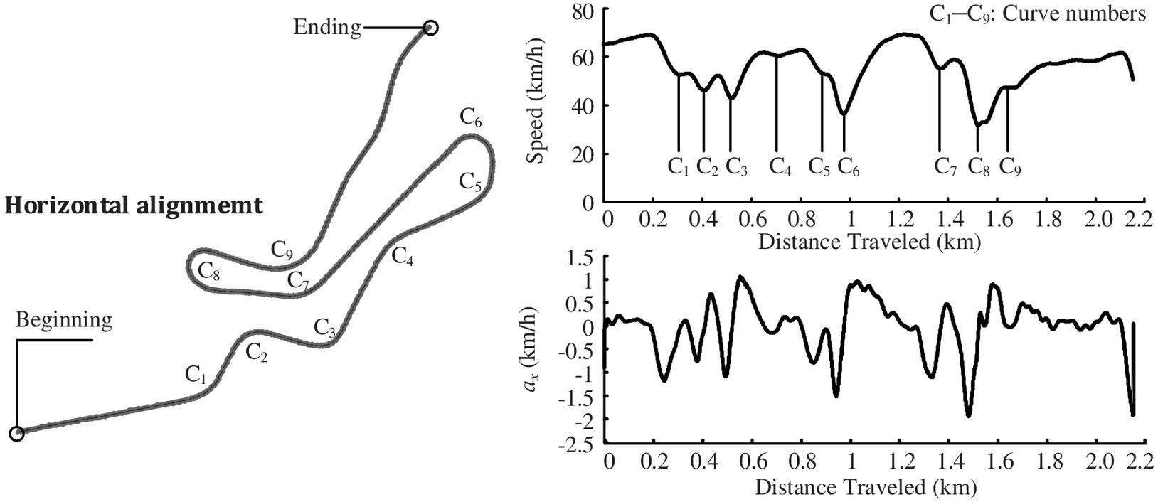
Fig. 9 shows the scatter plots generated from the data collected from the onboard passenger car tests. The sample size of the data is 534, and the sample size of the bends is 132 because two or three drivers make a round trip on the test roads (i.e., one bend can produce multiple test data points). Driving speed of the passenger car is not sensitive to the slope of the roadway (Xu et al. 2012), so the relationship between the acceleration/deceleration and horizontal alignment rather than the vertical alignment is analyzed.
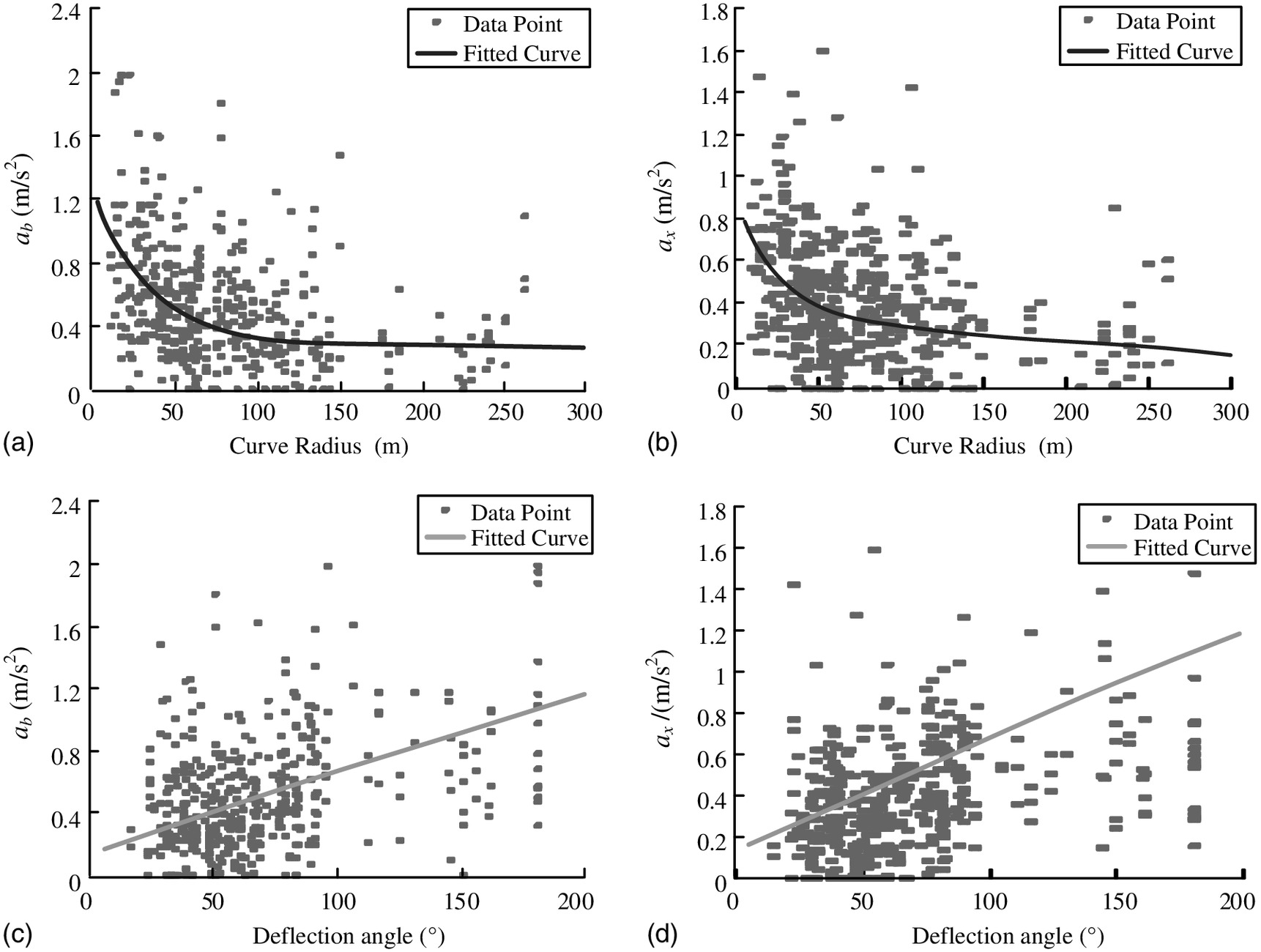
The plots in Figs. 9(a and b) show a rather strong negative correlation between acceleration/deceleration and the curve radius. This indicates that a driver entering a curve with a smaller radius will brake harder and will tend to accelerate faster as the vehicle leaves the curve. The reason for this is that curves with smaller radii have lower critical safe speed limits, so drivers must reduce their speed to a greater degree, which requires greater deceleration. When exiting one of these sharper curves, the difference between the driver’s desired speed and the vehicle’s actual speed is greater, so the driver will often use greater acceleration to increase his speed more quickly. The trend that is evident in the figure provides a reasonable basis for developing a model that relates acceleration/deceleration to the curve radius . After comparing the fitting accuracies of functions with different forms, the following two equations were found to yield fairly good results:
(2)
(3)
Figs. 9(c and d) show the scatter plots of the acceleration/deceleration rate and curve deflection angle. In contrast to the correlation observed for the curve radius, a positive correlation is evident between acceleration/deceleration and the curve angle. The larger the deflection angle, the harder the driver tends to brake and accelerate while entering and exiting the curve, respectively. The reason for this can be explained as follows. Curves with larger deflection angles are likely to give the driver the impression of being sharp and to adversely affect driving observations from the vehicle. Thus, drivers tend to choose a lower speed while negotiating such curves, resulting in greater deceleration. Eqs. (4) and (5) represent the regression models obtained from the scatter plots using the least-squares method.
(4)
(5)
In Eqs. (2)–(5), and = deceleration while entering a curve and the acceleration while exiting a curve, respectively; = horizontal curve radius; and = deflection angle of the horizontal curve, expressed in degrees.
The four formulas mentioned above can be used in operating speed model calculations and calibrations for the acceleration/deceleration of passenger cars on two-lane mountain highways, instead of setting the acceleration/decoration rate to a fixed value, as mentioned previously in “Acceleration/Deceleration Distribution Characteristics for Passenger Cars.” Together with horizontal curve speed models and desired speed models, these formulas make up a relatively complete system of operating speed models.
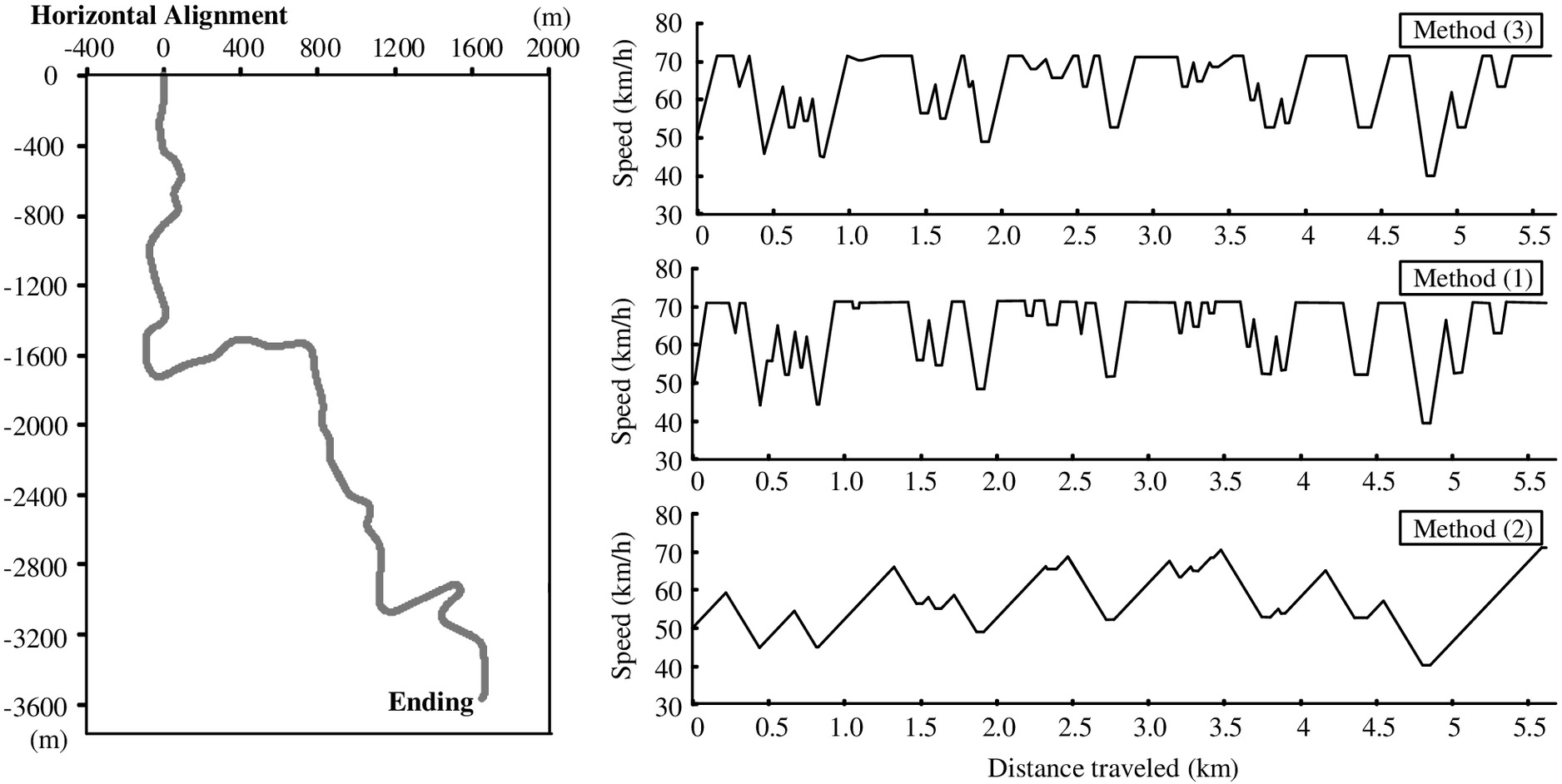
Fig. 10 illustrates the differences in operating speed profiles produced by three acceleration/deceleration calibration methods for a 5.5-km segment of the Anlong–Ceheng Section of Highway S313. The first method uses and (Echaveguren and Basualto 2003; Perco and Robba 2012), the second method uses and (China’s Highway Safety Audit Guidelines, JTG/TB05-2015), and the third method uses the values of and determined from Eqs. (2) and (3) developed in this study.
Conclusions and Future Research
The calibration and modeling of vehicle acceleration/deceleration rates are important aspects of constructing a complete operating speed model system. To determine the actual acceleration characteristics of vehicles, onboard driving tests and external observations were carried out on six two-lane mountain highways with complex shapes. The acceleration/deceleration characteristics of different types of vehicles were determined, and based on these characteristics, models relating acceleration/deceleration to road features were developed. The main conclusions are as follows:
1.
For passenger cars, the deceleration rate was greater than the acceleration rate. It is therefore unreasonable to assign a single value to both these rates. Instead, acceleration and deceleration need to be calibrated separately. Moreover, the existing calibrated values are apparently underestimated for mountain highways.
2.
The breakpoints on the acceleration/deceleration cumulative frequency curves did not appear at the 85th percentile. Rather, they were observed close to the 95th percentile. Therefore, the common practice of using the 85th percentile in mountain highway design should be reconsidered.
3.
The maximum acceleration and deceleration rates for coaches were very similar. For heavy trucks, the deceleration rate was clearly greater than the acceleration rate, and the acceleration and deceleration rates of coaches were both greater than those of heavy trucks.
4.
For passenger cars negotiating curves on two-lane mountain highways, a negative correlation existed between acceleration/deceleration and the curve radius, and a positive correlation existed between acceleration/deceleration and the deflection angle. Data collected in this study were used to develop an acceleration/deceleration—radius model and acceleration/deceleration—deflection angle model.
Future work: In the present study, only passenger cars were considered while developing the models relating acceleration/deceleration to curve features. The authors are currently carrying out continuous onboard driving tests using heavy trucks. Models relating the acceleration/deceleration of heavy trucks to the geometric features of roads will be established when sufficient data have been obtained.
Notation
The following symbols are used in this paper:
- algebraic difference of vertical grades (%);
- ADT
- average daily traffic ();
- 85th percentile acceleration rate ();
- CCR
- curvature change rate ();
- degree of curve (degrees);
- deflection angle (degrees);
- , deflection angle for curves 1 and 2 of compound curve (degrees);
- 85th percentile deceleration rate ();
- upper elevation rate (%)
- vertical grade (%);
- gradient preceding the curve (%);
- gradient succeeding the curve (%);
- INT
- intersection indicator;
- length of vertical curve for 1% change in grade ();
- length of curve (m);
- length of tangent (m);
- distance between horizontal and vertical point intersection (m);
- length of preceding tangent (m);
- length of succeeding tangent (m);
- length of vertical curve (m);
- lane width (m);
- maximum 85th percentile speed on approach tangent ();
- pavement condition;
- radius of curve (m);
- radius of preceding curve (m);
- radius of succeeding curve (m);
- shoulder width (m);
- RES
- number of residential driveways per km;
- maximum speed reduction from tangent to middle of curve ();
- 85th percentile speed ();
- 85th percentile speed on middle curve ();
- 85th percentile speed on tangent ();
- 85th percentile speed on the beginning of curves ();
- 85th percentile speed on the ending of curves ();
- 85th percentile speed on preceding curve ();
- maximum speed on tangent ();
- desired speed ();
- approach tangent speed ();
- curve approach speed ();
- posted speed limit ();
- percentile speed differential calculated as different between on two elements; and
- roadway width (m).
Acknowledgments
This research was supported by the National Natural Science Foundation of China (Grant No. 51278514), Applied Basic Research Program of the Ministry of Transport of China (Grant No. 2015319814050), and Science and Technology Planning Project of ChongQing Municipality, China (Grant No. Cstc2014jcyjA30024).
References
Abbas, S. K. S., Adnan, M. A., and Endut, I. R. (2011). “Exploration of 85th percentile operating speed model on horizontal curve: A case study for two-lane rural highways.” Procedia Social Behav. Sci., 16, 352–363.
Altamira, A., Garc, Y., Echaveguren, T., and Marcet, J. (2014). “Acceleration and deceleration patterns on horizontal curves and their tangents on two-lane rural roads.” Proc., Transportation Research Board 93rd Annual Meeting, Transportation Research Board, Washington, DC.
Camacho-Torregrosa, F. J., Pérez-Zuriaga, A. M., Campoy-Ungría, J. M., and García-García, A. (2013). “New geometric design consistency model based on operating speed profiles for road safety evaluation.” Acci. Anal. Prev., 61(8), 33–42.
Cardoso, J. L., et al. (1998). “Improvements of models on the relations between speed and road characteristics.” Task 5.3. SAFESTAR, Laboratorio Nacional de Engenharia Civil, Lisboa, Portugal.
Castro, M., Iglesias, L., Rodríguez-Solano, R., and Sánchez, J. A. (2008). “Highway safety analysis using geographic information systems.” Proc. Inst. Civ. Eng. Transp., 161(2), 91–97.
Castro, M., Sánchez, J. F., Sánchez, J. A., and Iglesias, L. (2011). “Operating speed and speed differential for highway design consistency.” J. Transp. Eng., 837–840.
Christopher, M., and Mason, J. M. (1995). “Geometric design guidelines to achieve desired operating speed on urban streets.” Proc., 65th ITE Annual Meeting: 1995 Compendium of Technical Papers, Institute of Transportation Engineers, Washington, DC.
Crisman, B., Marchionna, A., Perco, P., and Roberti, R. (2005). “Operating speed prediction model for two-lane rural roads.” Proc., 3rd Int. Symp. on Highway Geometric Design, Transportation Research Board, Washington, DC.
Dell’Acqua, G., Esposito, T., Lamberti, R., and Abate, D. (2007). “Operating speed mode on tangents of two-lane rural highways.” Proc., Int. SIIV Congress, Kirilo Savic Institute, Belgrade, Serbia.
Donnell, E. T., Ni, Y., Adolini, M., and Elefteriadou, L. (2001). “Speed prediction models for trucks on two-lane rural highways.” Transp. Res. Rec. Transp. Res. Board, 1751, 44–55.
Easa, S. M., and Mehmood, A. (2007). “Establishing highway horizontal alignment to maximize design consistency.” Can. J. Civ. Eng., 34(9), 1159–1168.
Echaveguren, T., and Basualto, J. (2003). “Consistency analysis of acceleration rate on the horizontal alignment with a configuration of simple elements.” Proc., XI Congreso Chileno de Ingeniería de Transporte, Universidad de Concepción, Santiago, Chile.
Fang, J., Wang, S. J., Zhu, Z. D., and Zhou, R. G. (2010). “Operating speed models for trucks at expressway tunnel sections.” J. Traffic Transp. Eng., 10(3), 90–94 (in Chinese).
Fitzpatrick, K., et al. (2000). “Speed prediction for two-lane rural highways.”, Federal Highway Administration, Washington, DC.
Fitzpatrick, K., Miaou, S. P., Brewer, M., Carlson, P., and Wooldridge, M. D. (2005). “Exploration of the relationships between operating speed and roadway features on tangent sections.” J. Transp. Eng., 261–269.
Gao, J. P., Kong, L. Q., Guo, Z. Y., and Wu, Z. H. (2004). “Study on operating speed of vehicles on expressway.” J. Chongoing Jiaotong Univ., 23(4), 78–81.
Gibreel, G. M., Easa, S. M., and El-Dimeery, I. A. (2001). “Prediction of operating speed on three-dimensional highway alignments.” J. Transp. Eng., 21–30.
Glennon, J. C., Neuman, T. R., and Leisch, J. E. (1986). “Safety and operational consideration for design of rural highways curves.”, Federal Highway Administration, McLean, VA.
Guidelines for the Design of Roads. (1984). “Guidelines for the design of roads.”, German Road and Transportation Research Association, Berlin.
Hashim, I. H., Abdel-Wahed, T. A., and Moustafa, Y. (2016). “Toward an operating speed profile model for rural two-lane roads in Egypt.” J. Traffic Transp. Eng., 3(1), 82–88.
Highway Capacity Manual. (2010). “Highway capacity manual 2010.”, Transportation Research Board of the National Academies, Washington, DC.
Islam, M. N., and Seneviratne, P. N. (1994). “Evaluation of design consistency of two-lane rural highways.” ITE J., 64(2), 28–31.
Jacob, A., and Anjaneyulu, M. V. L. R. (2013). “Operating speed of different classes of vehicles at horizontal curves on two-lane rural highways.” J. Transp. Eng., 287–294.
Kanellaidis, G., Golias, J., and Efstathiadis, S. (1990). “Driver’s speed behavior on rural road curves.” Traffic Eng., and Control, 31(7/8), 414–415.
Kerman, J. A., McDonald, M., and Mintsis, G. A. (1982). “Do vehicles slow down on bends? A study into road curvature, driver behaviour and design.” Proc., 10th Summer Annual Meeting, PTRC, Warwick Univ., Coventry, U.K.
Krammes, R. A., et al. (1995). “Horizontal alignment design consistency for rural two-lane highways.”, Federal Highway Administration, McLean, VA.
Lamm, R., and Choueiri, E. M. (1987). “Recommendations for evaluating horizontal design consistency based on investigations in the state of New York.” Transp. Res. Rec., 1122, 68–78.
Lamm, R., Choueiri, E. M., and Hayward, J. C. (1988). “Tangent as an independent design element.” Transp. Res. Rec., 1195, 13–20.
Lamm, R., Psarianos, B., Drymalitou, D., and Soilemezglou, G. (1995). Guidelines for the design of highway facilities, Vol. 3, Ministry for Environment, Regional Planning and Public Works, Athens, Greece.
Liu, J. P., Lin, S., and Gao, J. S. (2010). “Analysis and optimization for operating speed model on straight section on highway.” China J. Highw. Transp., 23(Sup), 83–88.
Luca, M. D., Russo, F., Cokorilo, O., and Dell’Acqua, G. (2014). “Modeling operating speed using artificial computational intelligence (ACI) on low-volume road.” Proc., Transportation Research Board 93rd Annual Meeting, Transportation Research Board, Washington, DC.
McFadden, J., and Elefteriadou, L. (2000). “Evaluating horizontal alignment design consistency of two-lane rural highways: Development of new procedure.” Transp. Res. Rec., 1737, 9–17.
Misaghi, P., and Hassan, Y. (2005). “Modeling operating speed and speed differential on two-lane rural roads.” J. Transp. Eng., 408–418.
Montella, A., Pariota, L., Galante, F., Imbriani, L., and Mauriello, F. (2014). “Prediction of drivers’ speed behaviour on rural motorways based on an instrumented vehicle study.” Transp. Res. Rec., 2434, 52–62.
Moon, S., and Yi, K. (2008). “Human driving data-based design of a vehicle adaptive cruise control algorithm.” Veh. Syst. Dyn., 46(8), 661–690.
Morrall, J., and Talarico, R. J. (1994). “Side friction demanded and margins of safety on horizontal curves.” Transp. Res. Rec., 1435, 145–152.
Nie, B., and Hassan, Y. (2007). “Modeling driver speed behavior on horizontal curves of different road classifications.” Proc., 86th Annual Meeting, Transportation Research Board, Washington, DC.
Ottesen, J. L., and Krammes, R. A. (1994). “Speed profile model for a U.S. operating speed-based consistency evaluation procedure.” Proc., 73rd Annual Meeting, Transportation Research Board, Washington, DC.
Ottesen, J. L., and Krammes, R. A. (2000). “Speed profile model for a design consistency evaluation procedure in the United States.” Transp. Res. Rec. Transp. Res. Board, 1701, 76–85.
Passetti, K. A., and Fambro, D. B. (1999). “Operating speeds on curves with and without spiral transitions.” Transp. Res. Rec., 1658, 9–16.
Perco, P., and Robba, A. (2012). “Evaluation of the deceleration rate for the operating speed-profile model.” ⟨http://www.siiv.net/site/sites/default/files/Documenti/bari2005/060.pdf⟩ (Feb. 6, 2016).
Richl, L., and Sayed, T. (2005). “Effect of speed prediction models and perceived radius on design consistency.” Can. J. Civ. Eng., 32(2), 388–399.
Richl, L., and Sayed, T. (2011). “Effect of speed prediction models and perceived radius on design consistency.” Can. J. Civ, Eng., 32(2), 388–399.
Setra, D. (1986). “Driving speed and road geometry.”, Ministère de l’ Equipment, du Logement, de l’ Aménagement du Territoire et des Transports, France.
Seungwuk, M., and Kyongsu, Y. (2008). “Human driving data-based design of a vehicle adaptive cruise control algorithm.” Vehicle Syst. Dyn., 46(8), 661–690.
Shao, Y. M., Mao, J. C., Liu, S. C., and Xu, J. (2011). “Analysis of speed control behavior for driver on mountain highway.” J. Traffic Transp. Eng., 11(1), 79–88.
Shao, Y. M., Xu, J., Li, B. W., and Yang, K. (2015). “Modeling the speed choice behaviors of drivers on mountainous roads with complicated shapes.” Adv. Mech. Eng., 7(2), 1–13.
TAC (Transportation Association of Canada). (1999). “Geometric design guide for Canadian roads.” Ottawa.
Tokunaga, R. A., Asano, M., Munehiro, K., Hagiwara, T., Kunugiza, K., and Kagaya, S. (2005). “Effects of curve designs and road conditions on driver’s curve sharpness judgment and driving behavior.” J. East. Asia Soc. Transp. Stud., 6, 3536–3550.
Vereingung Schweizerischer Strassenfachleute. (1992). “Speed-based highway alignment design.”, Zurich, Switzerland.
Voigt, A. P. (1996). “An evaluation of alternative horizontal curve design approaches for rural two-lane highways.”, Texas Transportation Institute (TTI), Texas A&M Univ., College Station, TX.
Xu, J., Shao, Y. M., Peng, Q. Y., and Chen, Y. X. (2012). “Driving speed investigation of single car or bus on different type of highways.” J. Transp. Sci. Eng., 28(4), 45–58.
Xu, J., Shao, Y. M., Zhao, J., and Yang, K. (2015). “Speed prediction model of heavy truck driving on curved segment with a slope of mountainous highway.” J. Chang’An Univ., 35(2), 67–74.
Zhang, Z. Y., Hao, X. Y., Wu, W. B., and Wang, D. (2014). “Research on the running speed prediction model of interchange ramp.” Procedia Social Behav. Sci., 138, 340–349.
Information & Authors
Information
Published In
Journal of Transportation Engineering, Part A: Systems
Volume 143 • Issue 7 • July 2017
Copyright
This work is made available under the terms of the Creative Commons Attribution 4.0 International license, http://creativecommons.org/licenses/by/4.0/.
History
Received: Mar 20, 2016
Accepted: Dec 7, 2016
Published online: Mar 6, 2017
Published in print: Jul 1, 2017
Discussion open until: Aug 6, 2017
Authors
Metrics & Citations
Metrics
Citations
Download citation
If you have the appropriate software installed, you can download article citation data to the citation manager of your choice. Simply select your manager software from the list below and click Download.