LEO Augmentation in Large-Scale Ionosphere-Float PPP-RTK Positioning

Wang, Kan; El-Mowafy, Ahmed; Cheng, Fang; Yang, Xuhai

doi:10.1061/JSUED2.SUENG-1414

Open access

Technical Papers

Jan 4, 2024

LEO Augmentation in Large-Scale Ionosphere-Float PPP-RTK Positioning

Authors: Kan Wang https://orcid.org/0000-0001-5688-6937 [email protected], Ahmed El-Mowafy https://orcid.org/0000-0001-7060-4123 [email protected], Fang Cheng [email protected], and Xuhai Yang [email protected]Author Affiliations

Publication: Journal of Surveying Engineering

Volume 150, Issue 2

https://doi.org/10.1061/JSUED2.SUENG-1414

PDF

Abstract

Precise point positioning-real-time kinematic (PPP-RTK) positioning combines the advantages of PPP and RTK, which enables the integer ambiguity resolution (IAR) without requiring a reference station nearby. The ionospheric corrections are delivered to users to enable fast IAR. For large-scale networks, precise interpolation of ionospheric delays is challenging. The ionospheric delays are often independently estimated by the user, in the so-called ionosphere-float mode. The augmentation of low Earth orbit (LEO) satellites can bridge this shortcoming thanks to their fast speeds and the resulting rapid geometry change. Using 30-s real dual-frequency Global Positioning System (GPS) and Beidou Navigation Satellite System (BDS) observations within a large-scale network of thousands of kilometers, this contribution tests the effects of LEO augmentation using simulated dual-frequency LEO signals from the navigation-oriented LEO constellation, CentiSpace. Results showed that the LEO augmentation makes the solution convergence less sensitive to the original Global Navigation Satellite System (GNSS)-based model strength. The improvements in the convergence times are significant. For example, in the kinematic mode, the convergence time of the 90% lines of the GPS/BDS-combined ambiguity-float horizontal solutions to 0.05 m is shortened from more than 60 to 3.5 min, and that of the GPS-only partial ambiguity resolution (PAR)-enabled horizontal solutions is shortened from more than 20 to 4.5 min. In both the ambiguity-float and PAR-enabled cases, the 68.27% (

1 σ

) lines of both the kinematic and static horizontal and height errors can converge to 0.05 m within 4 min, and for the 90% lines, within 6.5 min in all cases. The 90% line of the GPS/BDS/LEO combined PAR-enabled solutions can converge to 0.05 m within 2.5 and 3 min in the horizontal and up direction, respectively. Results also showed that enlarged projection of the mismodeled biases on the user coordinates were observed in the LEO-augmented scenario after convergence or ambiguity resolution. This is mainly due to the lower orbital height and low elevation angles of the LEO satellites, which requires further research when real LEO navigation signals are available.

Introduction

The precise point positioning-real-time kinematic (PPP-RTK) positioning method, which was first introduced by Wübbena et al. (2005), combines the advantages of both the precise point positioning (PPP) and real-time kinematic (RTK) positioning techniques. With a regional network providing satellite clocks, satellite phase biases, and optionally ionospheric delays to users, integer ambiguity resolution (IAR) is enabled while avoiding, to some extent, the users’ need for nearby infrastructure as generally adopted in RTK positioning. Diverse studies have been performed to recover the integer nature of the ambiguities in precise positioning (Collins 2008; Ge et al. 2008; Geng et al. 2010; Teunissen et al. 2010), and a review has been given by Teunissen and Khodabandeh (2015).

Among all the different techniques enabling the IAR in the PPP, the Undifferenced and Uncombined (UDUC) model applied in the PPP-RTK has shown its advantages in the possibilities to strengthen the observation model by adding spatial and temporal constraints in otherwise eliminated parameters, and flexibly extending the model in any number of frequencies (Odijk et al. 2015). In addition to the satellite clocks and phase biases, ionospheric delays can be optionally delivered to users to accelerate the IAR and thus the convergence of the user positioning solutions (Odijk et al. 2012). In large-scale networks with interstation distances of thousands of kilometers, however, the high-precision ionosphere interpolation remains a challenge. In such a case, the so-called ionosphere-float model is often utilized, where users do not use the ionosphere information delivered by the network, but estimate the ionospheric delays by themselves. The situation may also apply to networks with smaller scales because the ionospheric conditions vary with geographical locations and time, and suffer from huge anomalies in solar active years reaching, e.g.,

412 mm / km

in northern Ohio in November 2003 (Pullen et al. 2009). The ionospheric interpolation in such cases becomes a problem for applications requiring high reliability, e.g., intelligent transport systems (ITS) (Hassan et al. 2020).

When applying the ionosphere-float model, the interpolation errors of the ionospheric delays are avoided, resulting, however, in a longer convergence time (Odijk et al. 2016; Nadarajah et al. 2018; Psychas and Verhagen 2020) due to the weakened observation model and the slow geometry change of the Global Navigation Satellite System (GNSS) satellites flying typically at medium Earth orbits (MEOs). The low Earth orbit (LEO) satellites can bridge this shortcoming. Due to the much lower altitudes of LEO satellites at hundreds to about 1,500 km (Montenbruck and Gill 2000), LEO satellites are flying at a much faster speed than the GNSS satellites. The faster speed of LEO satellites leads to a more rapid geometry change of satellites with respect to users on Earth.

Various studies have investigated the benefits of LEO augmentation in reducing the PPP convergence time and ambiguity resolution (Ge et al. 2018; Li et al. 2018, 2019, 2023; Zhao et al. 2020; Hong et al. 2023). Ge et al. (2018) and Li et al. (2018, 2023) demonstrated that LEO augmentation could significantly shorten the convergence time of the traditional PPP, i.e., from tens of minutes to only a few minutes or even less. Li et al. (2019) and Hong et al. (2023) showed the strong benefits of LEO augmentation in shortening the time to first fix (TTFF) in GNSS-based PPP and PPP-RTK ambiguity resolution. Additionally, Zhao et al. (2020) exhibited a reduced convergence time and improved accuracy of the LEO-augmented ambiguity float and fixed PPP under harsh environments. The reduced convergence time was also observed in the ambiguity-float horizontal positioning precision in the ionosphere-weighted PPP-RTK positioning (Wang et al. 2022a).

The same can be expected for the IAR-enabled ionosphere-float PPP-RTK solutions, where the rapid geometry change can bridge the lack of the ionospheric corrections, accelerate the IAR (Nardo et al. 2016), and as a result, accelerate the convergence of the positioning results to high accuracy. In addition to the convergence time, the high number of LEO satellites also greatly increases the satellite visibility and the position dilution of precision (PDOPs) (Wang et al. 2022a), which benefits the measurement geometry and strengthens the observation model in general. The faster convergence time is expected due to the faster satellite geometry change brought by LEO satellites. However, high-accuracy ionospheric interpolation may still remain a problem when allowing LEO satellites to join the network processing, without increasing the density of network stations.

Every coin has two sides. Despite the aforementioned advantages, the characteristics of LEO satellites also have disadvantages in PPP-RTK positioning. Compared with the much higher GNSS satellites, the LEO satellites’ orbital errors might influence the PPP-RTK solutions more due to their lower altitudes, even when using a network of the same scale. The smaller footprints of LEO satellites (Cakaj et al. 2014) lead to fewer stations that can simultaneously view the same satellite, i.e., having lower precision of the LEO-satellite-related network corrections. The short visible time span of 5–20 min (Perez 1998) for LEO satellites would also hamper the convergence of their network corrections. The LEO satellites flying at low elevation angles, which occupy a significant portion of all the visible LEO satellites for the CentiSpace constellation used in this contribution as an example (Wang et al. 2022a), would also imply larger noise in the observations.

Considering all the advantages and disadvantages, this contribution reveals the influences of LEO augmentation on ionosphere-float PPP-RTK solutions. In addition to real multiconstellation GNSS data of the Global Positioning System (GPS) and the Beidou Navigation Satellite System (BDS), simulated LEO dual-frequency L1/L5 observations are used based on the CentiSpace constellation, a navigation-oriented LEO constellation that has registered its orbital characteristics in the International Telecommunication Union (ITU) (Yang 2019; Wang et al. 2022a). The study will analyze to which extent LEO augmentation can benefit the ionosphere-float GNSS-based PPP-RTK solutions.

The paper starts with a short explanation of the UDUC model applied on both the network and user sides. The setup for data analysis will be introduced afterward, including the GNSS network and user distributions and the simulations of the LEO satellite signals. The user positioning results are then analyzed and discussed for the GNSS-only and GNSS/LEO combined scenarios. The conclusion is given at the end.

Processing Strategy

This section is split into two subsections, introducing the UDUC model at the network and user parts.

Network Model

At the network part, the phase (

Δ φ_{r, j}^{s}

) and code (

Δ p_{r, j}^{s}

) observed-minus-computed (O-C) terms without rank deficiencies can be formulated as follows:

E (Δ φ_{r, j}^{s}) = g_{r}^{s} Δ τ_{r} + d {\tilde{t}}_{r, g} - d {\tilde{t}}^{s} - μ_{j} {\tilde{ι}}_{r, g}^{s} + {\tilde{δ}}_{r, j, g} - {\tilde{δ}}_{, j}^{s} + λ_{j} {\tilde{N}}_{r, j}^{s}

(1)

E (Δ p_{r, j}^{s}) = g_{r}^{s} Δ τ_{r} + d {\tilde{t}}_{r, g} - d {\tilde{t}}^{s} + μ_{j} {\tilde{ι}}_{r, g}^{s} + {\tilde{d}}_{r, j, g} - {\tilde{d}}_{, j}^{s}

(2)

where subscripts

r

,

j

, and

g

= corresponding receiver, frequency, and constellation; superscript

s

= corresponding satellite;

g_{r}^{s}

= mapping function of the wet tropospheric delays, here, the Ifadis mapping function (Ifadis 1986);

Δ τ_{r}

= wet part of the zenith tropospheric delays (ZTDs) to be estimated;

μ_{j}

= frequency-dependent factor

f_{1}^{2} / f_{j}^{2}

, with

f_{j}

denoting the

j

th frequency in the corresponding constellation; and

λ_{j}

denoting its wavelength; and

E (\cdot)

= expectation operator to ignore the observation noise in the equations.

A continuously operating reference station (CORS) network is used here with station coordinates known and fixed in the observation equations. Corrected in the O-C terms are also the hydrostatic tropospheric delays computed based on the Ifadis model, the phase center offsets (PCOs) and phase center variations (PCVs) of receivers and satellites based on the igs14.atx (Rebischung and Schmid 2016), and the phase windups (Wu et al. 1993). High-precision real-time satellite orbits are introduced in the estimation, which will be explained in the next section. The network processing considers the all-in-view satellite observations (Zhang et al. 2022).

From Eqs. (1) and (2), it can be observed that except for the ZTD

Δ τ_{r}

, all estimable parameters with a tilde sign above the symbols, i.e., the receiver clock bias

d {\tilde{t}}_{r, g}

(in range), the satellite clock bias

d {\tilde{t}}^{s}

(in range), the ionospheric delays

{\tilde{ι}}_{r, g}^{s}

on L1, the receiver and satellite phase biases

{\tilde{δ}}_{r, j, g}

and

{\tilde{δ}}_{, j}^{s}

, their counterparts for the code observations

{\tilde{d}}_{r, j, g}

and

{\tilde{d}}_{, j}^{s}

, and the ambiguity

{\tilde{N}}_{r, j}^{s}

, are newly formed based on the

S

-system theory to avoid singularities and rank deficiencies (Baarda 1981; Teunissen 1985). Satellite

s

distinguishes among all used constellations, and the constellation-specific subscript

g

is thus not given for the satellite-related parameters. With the ambiguities and all hardware biases linked in time, the formulations of these estimable parameters are given in Table 1 (Odijk et al. 2015). The

Δ τ_{r}

is also linked in time, but does not influence the formulation of the estimable parameters here. The parameters

d t_{1} (t_{i})

,

d_{1, j, g} (t_{1})

,

δ_{1, j, g} (t_{1})

,

N_{1, j}^{s} (t_{i})

,

N_{r, j, g}^{1} (t_{i})

,

d_{r \neq 1, j = 1, 2, g} (t_{1})

, and

d_{, j = 1, 2}^{s} (t_{1})

serve as

S

-basis parameters and are thus not estimated with their biased terms in Table 1. The subscripts IF and GF denote the ionosphere-free and geometry-free combination of the corresponding parameters as follows:

{(\cdot)}_{, IF} = \frac{μ_{2} {(\cdot)}_{, 1} - μ_{1} {(\cdot)}_{, 2}}{μ_{2} - μ_{1}}

(3)

{(\cdot)}_{, GF} = \frac{{(\cdot)}_{, 2} - {(\cdot)}_{, 1}}{μ_{2} - μ_{1}}

(4)

Table 1. Formulations of the estimable parameters during the network processing

Estimable parameter	Formulation
$d {\tilde{t}}_{r, g} (t_{i})$	$d t_{1 r} (t_{i}) + d_{1 r, IF, g} (t_{1})$
$d {\tilde{t}}^{s} (t_{i})$	$d t^{s} (t_{i}) + d_{, IF}^{s} (t_{1}) - d t_{1} (t_{i}) - d_{1, IF, g} (t_{1})$
${\tilde{ι}}_{r, g}^{s} (t_{i})$	$ι_{r}^{s} (t_{i}) + d_{r, GF, g} (t_{1}) - d_{, GF}^{s} (t_{1})$
${\tilde{δ}}_{r, j, g} (t_{i})$	$δ_{r, j, g} (t_{i}) - δ_{1, j, g} (t_{1}) + μ_{j} d_{1 r, GF, g} (t_{1}) - d_{1 r, IF, g} (t_{1}) + λ_{j} N_{1 r, j, g}^{1} (t_{i})$
${\tilde{δ}}_{, j}^{s} (t_{i})$	$δ_{, j}^{s} (t_{i}) + μ_{j} (d_{, GF}^{s} (t_{1}) - d_{1, GF, g} (t_{1})) - d_{, IF}^{s} (t_{1}) + d_{1, IF, g} (t_{1}) - δ_{1, j, g} (t_{1}) - λ_{j} N_{1, j}^{s} (t_{i})$
${\tilde{d}}_{r, j, g} (t_{i})$	$d_{r, j, g} (t_{i}) - d_{1, j, g} (t_{1}) - d_{1 r, IF, g} (t_{1}) - μ_{j} d_{1 r, GF, g} (t_{1})$
${\tilde{d}}_{, j}^{s} (t_{i})$	$d_{, j}^{s} (t_{i}) - d_{, IF}^{s} (t_{1}) - μ_{j} d_{, GF}^{s} (t_{1}) - d_{1, j, g} (t_{1}) + d_{1, IF, g} (t_{1}) + μ_{j} d_{1, GF, g} (t_{1})$
${\tilde{N}}_{r, j}^{s} (t_{i})$	$N_{1 r, j}^{s} (t_{i}) - N_{1 r, j, g}^{1} (t_{i})$

Note: The ambiguities and all hardware biases are linked in time.

Based on Eqs. (3) and (4), we have

{(\cdot)}_{, j} = {(\cdot)}_{, IF} + μ_{j} {(\cdot)}_{, GF}

(5)

The temporal constraints differ for different estimable parameters. The ambiguities are assumed constant unless a cycle slip is detected. The hardware biases and ZTDs are constrained as random-walk processes with the corresponding spectral density parameters given in Table 2. These parameters are updated from one epoch to the next as follows:

\hat{x} (t_{i | i - 1}) = \hat{x} (t_{i - 1})

(6)

Q_{\hat{x}} (t_{i | i - 1}) = Q_{\hat{x}} (t_{i - 1}) + S_{x}

(7)

where

\hat{x} (t_{i | i - 1})

is the time-updated parameter vector; and

\hat{x} (t_{i - 1})

= their estimated values at

t_{i - 1}

. The variance-covariance (V-C) matrix of

\hat{x} (t_{i | i - 1})

, denoted as

Q_{\hat{x}} (t_{i | i - 1})

, is the sum of the V-C matrix of

\hat{x} (t_{i - 1})

from the last epoch, denoted as

Q_{\hat{x}} (t_{i - 1})

, and the system noise matrix

S_{x}

. For the parameters listed in Table 2, the

k

th diagonal element in

S_{x}

can be simply calculated with

q_{x_{k}}^{2} \times Δ t

, where

q_{x_{k}}

denotes the spectral density parameter of the

k

th parameter in

x

, and

Δ t

is the sampling interval of the observations.

Table 2. Temporal constraints applied to the estimable parameters

Parameter	Spectral density parameter ( $m / \sqrt{s}$ )
$Δ τ_{r}$	0.0001
${\tilde{δ}}_{, j}^{s} (t_{i})$ , ${\tilde{d}}_{, j}^{s} (t_{i})$	0.0001
${\tilde{δ}}_{r, j, g} (t_{i})$ , ${\tilde{d}}_{r, j, g} (t_{i})$	0.001
${\tilde{N}}_{r, j}^{s}$	0

Based on Eqs. (1), (2), (6), and (7), the ambiguity-float solutions of all the unknown estimable parameters can be solved with the least-squares adjustment. The standard deviations of the GNSS phase and code observations are assumed to be elevation-dependent as follows:

σ_{φ} = \frac{σ_{φ_{0}}}{\sin (θ_{e})}

(8)

σ_{p} = \frac{σ_{p_{0}}}{\sin (θ_{e})}

(9)

where

σ_{φ_{0}}

and

σ_{p_{0}}

= standard deviations of the zenith-referenced phase and code observations, respectively, which were set to 0.003 and 0.3 m in this study; and

θ_{e}

= elevation angle. Observations from different GNSS constellations could exhibit different zenith-referenced standard deviations under different measurement environments and when using different receiver/antenna types. In this study, a simplified setting of equal zenith-referenced standard deviation was used for observations from different constellations.

With the estimated float ambiguities and their V-C matrix, the ambiguities can be resolved to integers with the least-squares ambiguity decorrelation adjustment (LAMBDA) method (Teunissen 1993, 1995). Partial ambiguity resolution (PAR) (Nardo et al. 2016) is enabled in this contribution with a success rate (SR) threshold of 99.99% at the network part.

User Model

The satellite clocks (

d {\hat{\tilde{t}}}^{s}

), phase biases (

{\hat{\tilde{δ}}}_{, j}^{s}

), and in case of

j > 2

, the code biases

{\hat{\tilde{d}}}_{, j > 2}^{s}

processed at the network side are delivered to the users to help with their positioning. The phase and code observation equations at the user side can be formulated as follows:

E (Δ φ_{u, j}^{s} + d {\hat{\tilde{t}}}^{s} + {\hat{\tilde{δ}}}_{, j}^{s}) = {(G_{u}^{s})}^{T} Δ x_{u} + g_{u}^{s} Δ τ_{u} + d {\tilde{t}}_{u, g} - μ_{j} {\tilde{ι}}_{u, g}^{s} + {\tilde{δ}}_{u, j, g} + λ_{j} {\tilde{N}}_{u, j}^{s}

(10)

E (Δ p_{u, j}^{s} + d {\hat{\tilde{t}}}^{s} + {\hat{\tilde{d}}}_{, j > 2}^{s}) = {(G_{u}^{s})}^{T} Δ x_{u} + g_{u}^{s} Δ τ_{u} + d {\tilde{t}}_{u, g} + μ_{j} {\tilde{ι}}_{u, g}^{s} + {\tilde{d}}_{u, j, g}

(11)

where the subscript

u

= user;

Δ x_{u}

denotes the user coordinate increment vector; matrix

G_{u}^{s}

contains the satellite-to-user unit direction vectors; and

N_{u, j}^{1} (t_{i})

and

d_{u, j = 1, 2, g} (t_{1})

serve as

S

-basis parameters and are not estimated in their biased forms. The temporal constraints for

Δ τ_{u}

,

{\tilde{δ}}_{u, j}

,

{\tilde{d}}_{u, j}

, and

{\tilde{N}}_{u, j}^{s}

follow those given in Table 2. The PAR is enabled with a SR threshold set to 99.9% on the user side.

Data Processing

To assess the impact of the LEO augmentation in large-scale ambiguity-float PPP-RTK positioning, real GNSS observations and simulated LEO observations were used in this contribution. This section is split into two parts. The first part introduces the measurement setup of the network and user stations for the GNSS-based real data processing, and the second part explains the simulation of LEO signals.

GNSS Real Data

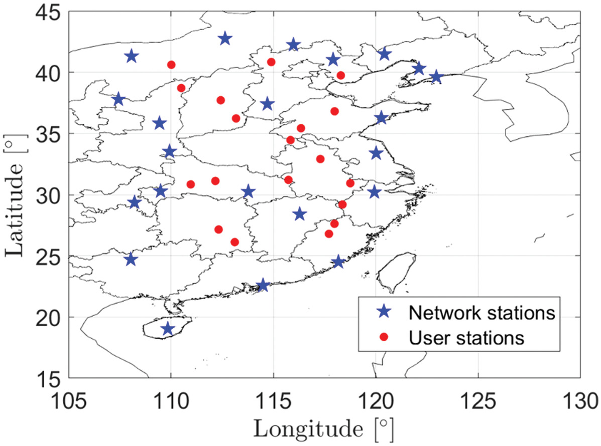
CORS stations were used for the PPP-RTK processing in this study. As shown in Fig. 1, the network and user stations are distributed from central to eastern China, including 22 network stations (blue stars) and 19 user stations (red dots). The network is around 2,500 km in the north–south direction, and around 1,300 km in the east–west direction. All stations are equipped with geodetic-grade multi-GNSS receivers and antennas, i.e., with the receiver types ComNav PDB38 (ComNav Technology, Shanghai, China) and Unicore UR380 (UniCore Communications, Beijing), and the antenna type HX-CGX601A (Harxon Corporation, Shenzhen, China).

Fig. 1. CORS stations used for the PPP-RTK network and user processing in our tests.

The GPS signals on L1C (1,575.42 MHz) and L2P (1,227.6 MHz), and the BDS signals on B1I (1,561.098 MHz) and B3I (1,268.52 MHz) on February 1, 2022, from 1:03:00 to 5:29:30 in GPS time (GPST) were used for the processing. The sampling interval was 30 s. The user processing started 3 h after the network processing to allow for the convergence of the network solutions. The user processing was performed in hourly sessions with the starting windows shifted by 30 s each time for all tested user stations. The user session was set not to exceed the end of the test period. The network processing was only computed once and not recomputed for each hourly user session. In total, nearly 800 hourly sessions without data gaps were considered in the statistical analysis. Both the network and the user processing were performed using the real-time orbital products provided by the National Centre for Space Studies (CNES) (Kazmierski et al. 2018). The elevation mask was set to 10°. The user coordinates

Δ x_{u}

were estimated in two modes:

•

static mode, with

Δ x_{u}

constrained as constant in time; and

•

kinematic mode, with no temporal constraint set to

Δ x_{u}

.

Fig. 2 shows the percentages of the numbers of used satellites per epoch for all network and user stations during their corresponding processing periods. The BDS geostationary (GEO) satellites were not considered in the processing due to their lower orbital accuracies than the MEO and inclined geosynchronous satellite orbit (IGSO) satellites with their very slow geometry changes to the Earth (Lv et al. 2020).

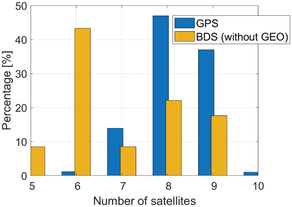
Fig. 2. Percentages of the numbers of the used satellites per epoch for dual-frequency GPS satellites on L1C and L2P and BDS satellites on B1I and B3I.

From Fig. 2, it can be observed that seven to nine GPS satellites are used most of the time, and around five to nine BDS MEO and IGSO satellites are usable on their selected two frequencies. The higher yellow bar at the BDS satellite number of six than that of seven and above is caused by the missing satellite orbits of C11 and C12 in the CNES real-time orbits on the test day.

Simulation of the LEO Satellite Signals

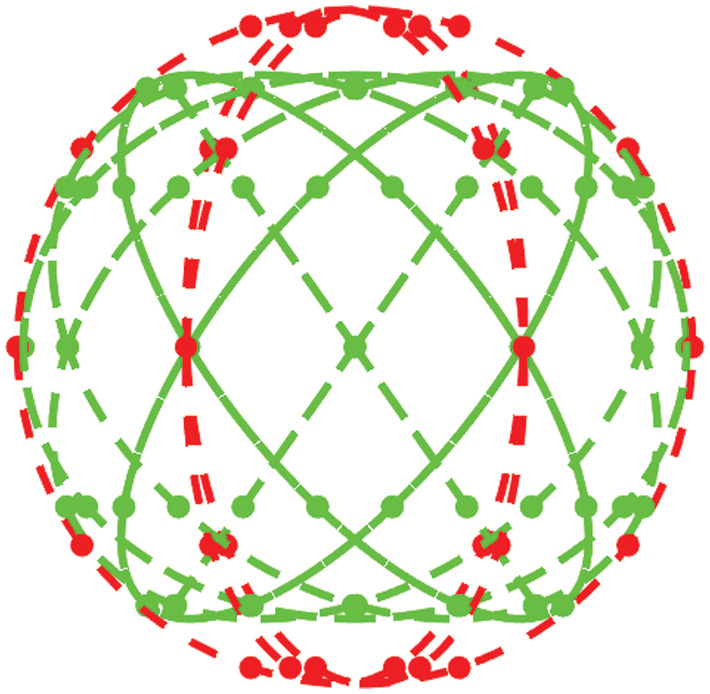
In this contribution, the navigation-oriented LEO satellite constellation CentiSpace (Yang 2019) was used for the simulation of LEO satellite signals. CentiSpace plans for circular orbits and follows the Walker constellation (Walker 1984). It has currently registered two orbital layers at the ITU as shown in Fig. 3, i.e., Layer A (green) follows the Walker Delta constellation, with 120 satellites on 12 orbital planes, with an orbital height of 975 km and an inclination of 55°; Layer B (red) follows the Walker Star constellation with 30 satellites on three orbital planes, with an orbital height of 1,100 km and an inclination of 87.4° (Wang et al. 2022a).

Fig. 3. CentiSpace LEO satellite configuration.

The CentiSpace satellites will broadcast GNSS interoperable phase and code signals on L1 (1,575.42 MHz) and L5 (1,176.45 MHz). As such, the dual-frequency phase (

φ_{r, j, L}^{s}

) and code signals (

p_{r, j, L}^{s}

) are simulated using

φ_{r, j}^{s} = X_{r} - X^{s} + g_{r}^{s} τ_{r} + d t_{r} - d t^{s} - μ_{j} ι_{r}^{s} + δ_{r, j, L} - δ_{, j}^{s} + λ_{j} N_{r, j}^{s} + φ_{tbc} + ϵ_{φ, r, j}^{s}

(12)

p_{r, j}^{s} = X_{r} - X^{s} + g_{r}^{s} τ_{r} + d t_{r} - d t^{s} + μ_{j} ι_{r}^{s} + d_{r, j, L} - d_{, j}^{s} + p_{tbc} + ϵ_{p, r, j}^{s}

(13)

where

X_{r}

and

X^{s}

= ground-truth coordinates of the stations and the LEO satellite orbits, respectively.

The wet part of the ZTDs

τ_{r}

were taken from the estimated ZTDs from the GPS/BDS-combined PAR-enabled network solutions containing all stations used in this study, allowing 1 h of convergence time before the start of the processing period in this study. The estimated ZTDs were further smoothed with a sliding window of 10 min and mapped onto the line-of-sight (LOS) direction with the Ifadis mapping function

g_{r}^{s}

, forming the simulated wet tropospheric delays in the LOS direction. The estimable receiver clock errors (

d {\tilde{t}}_{r, L}

) were estimated independently for the LEO constellation due to the involvement of

d_{1 r, IF, g} (t_{1})

(Table 1); thus, the values of the simulated receiver clock errors here (

d t_{r}

) will not influence the processing and were set to zeros. The satellite clock errors (

d t^{s}

) and the ionospheric delays (

ι_{r}^{s}

) were estimated as independent parameters in this study without applying any models. Their values will not influence the processing either and were set to zeros (Wang et al. 2022b).

The LEO satellite clocks were assumed to be estimated aligned with the time system of the GPS satellite clocks. For the LEO satellite observations, the receiver phase (

δ_{r, j, L}

) and code hardware biases (

d_{r, j, L}

) were simulated as random-walk processes with a temporal constraint of

0.001 m / \sqrt{s}

, and the LEO satellite phase (

δ_{, j}^{s}

) and code hardware biases (

d_{, j}^{s}

) were simulated as random-walk processes with a temporal constraint of

0.0001 m / \sqrt{s}

. The LEO satellite ambiguities

N_{r, j}^{s}

were set to zeros.

Here,

φ_{tbc}

and

p_{tbc}

represent the other phase- and code-related terms that were assumed to be corrected in the O-C terms, respectively. They included the satellite and receiver and satellite antenna sensor offsets, their PCO and PCV corrections, the hydrostatic part of the tropospheric delays, the relativistic effects, the solid Earth tide corrections, and the phase windups (only for phase). The

φ_{tbc}

and

p_{tbc}

terms’ values will not influence processing as long as the same corrections are considered in the computed terms. The simulated phase noise (

ϵ_{φ, r, j}^{s}

) and code noise (

ϵ_{p, r, j}^{s}

) followed the elevation-dependent weighting function in Eqs. (8) and (9), with the zenith-referenced phase and code standard deviations set to 0.002 and 0.2 m, respectively, due to possible multipath whitening and, accordingly, the smaller influences of the multipath biases.

Considering the disturbances of other mismodeled biases, such as the influences of the larger real-time orbital errors (to be discussed subsequently) and the simulated ZTDs biased from their true values, during the processing, the zenith-referenced standard deviations were also set to 0.003 and 0.3 m for phase and code, respectively, as mentioned in the “Processing Strategy” section. In practice, the LEO satellite signal noise behaviors with the whitened multipath effects under different measurement environments is an interesting topic to be studied when these signals are available in the future.

To generate the O-C terms for the processing, the computed part of the phase (

φ_{r 0, j, L}^{s}

) and code observations (

p_{r 0, j, L}^{s}

) are formulated as follows:

φ_{r 0, j, L}^{s} = X_{r 0} - X^{s 0} + φ_{tbc}

(14)

p_{r 0, j, L}^{s} = X_{r 0} - X^{s 0} + p_{tbc}

(15)

where

X_{r 0}

= ground-truth coordinates of the network stations and the a priori coordinates for the user stations; and

X^{s 0}

= LEO satellite orbits introduced in the processing, which are not equal to the true orbits (Hauschild et al. 2016; Montenbruck et al. 2021).

The introduced LEO satellite orbits were assumed to be real-time orbits, which can be, e.g., predicted in short-term based on high-precision postprocessed LEO satellite orbits using GNSS measurements tracked onboard. Fig. 4(a) shows the root-mean square (RMS) of the orbital prediction errors for the 811-km Sentinel-3B as an example of LEO satellites, based on more than 8,000 prediction samples collected in 2019 and 2020. Due to the air drag effects that are difficult to be perfectly modeled, the along-track errors are higher than the errors in the other two directions when extrapolating the orbits with dynamic models, leading to sub-decimeter (dm) to dm-level prediction errors within 30 min.

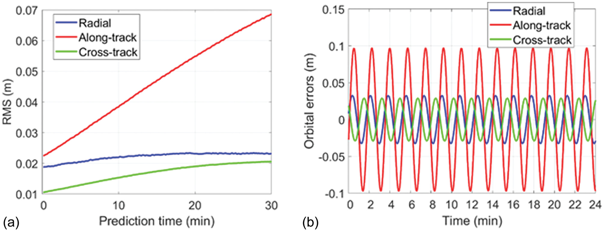
Fig. 4. (a) RMS of the orbital prediction errors of Sentinel-3B; and (b) the simulated real-time LEO satellite orbital errors for one example of the CentiSpace satellites on Layer A.

The CentiSpace orbits are higher than the Sentinel-3B orbits with smaller influences of the air drag. One can thus expect an orbital prediction behavior not worse than those shown in Fig. 4(a). Considering the half-hour prediction errors of Sentinel-3B, real-time LEO satellite orbital errors with RMS of 2.3, 6.9, and 2.1 cm were considered in the radial, along-track, and cross-track direction, respectively. Considering that dynamically estimated or extended LEO satellite orbits often show periodic behaviors at the level of the orbital periods due to model deficiencies, the orbital errors for satellite

s

in direction

d

, denoted as

Δ X_{d}^{s}

, were simulated with sine functions as follows:

Δ X_{d}^{s} = A_{d} \sin (\frac{2 π}{T_{L}} (t - t_{0}) + Δ ϕ_{d}^{s})

(16)

where

T_{L}

is set to the CentiSpace orbital periods, i.e., around 1.74 and 1.79 h for Layers A and B, respectively;

t

and

t_{0}

= time of the day and the start of the day in GPST, respectively; amplitude

A_{d}

= around 1.42 times the wanted RMS of the orbital errors in each direction, i.e., about 3.3, 9.7, and 2.9 cm in the radial, along-track, and cross-track directions, respectively; and

Δ ϕ_{d}^{s}

= phase shift. For different LEO satellites on the same layer, a phase shift of

(2 π k / 1,000) + (2 d π / 3)

is generated to distinguish the orbital errors of different satellites and in different directions, where

k

is a random number between 0 and 1,000, and

d = 0

, 1, 2 indicating the three directions.

The orbital errors simulated in the preceding paragraphs were added to the true orbits to form the introduced orbits

X^{s 0}

in Eqs. (14) and (15). The same orbits are introduced in the network and user processing, so that a significant part of the orbital errors can be reduced within a regional network.

Based on the increased signal strength and whitened multipath effects of the LEO satellite signals compared with those of GNSS satellites, the LEO satellite signals are considered to be more resistant to interferences, more capable of penetrating obstacles, and less influenced by mismodeled multipath biases. Thus, the elevation mask was set to 5°, i.e., lower than the 10° set for the GNSS signals.

Test Results

In this section, the ionosphere-float PPP-RTK solutions based on the network and users introduced in the “Data Processing” section are analyzed without and with the LEO augmentation. In the first subsection, the convergence of the ambiguity-float and PAR-enabled user coordinates are analyzed in detail for the GPS-only and GPS/BDS-combined solutions in both the kinematic and static modes. In the second subsection, the effects of LEO augmentation are discussed for the ambiguity-float and PAR-enabled solutions in both single- and dual-constellation scenarios.

GNSS-Based Real-Data Solutions without LEO Augmentation

The hourly user sessions were first processed using GPS-only L1 and L2 signals, having the network processing performed also using only the corresponding GPS measurements. Adding more satellite constellations in the network processing side does not benefit the GPS-related satellite products much because the only commonly estimated parameter for all constellations is ZTD there.

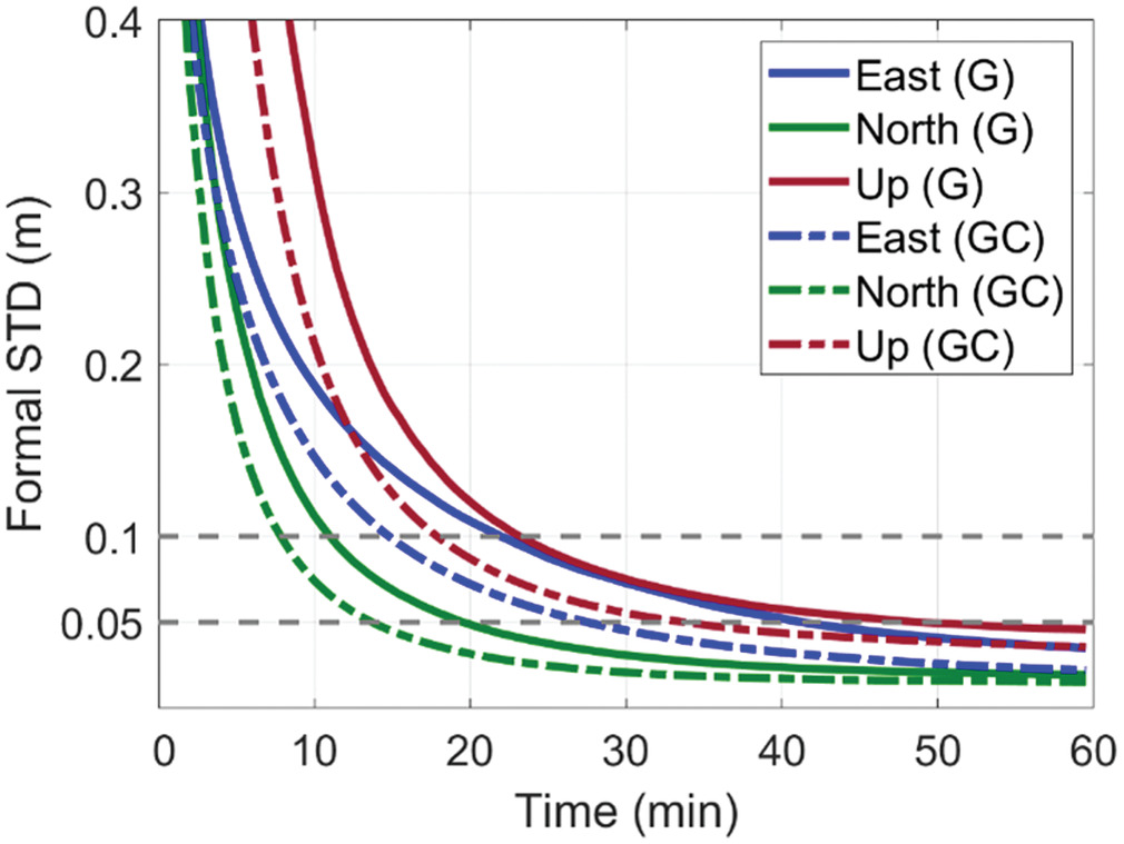
Fig. 5 shows the 68.27% (

1 σ

) and 90% lines of the absolute east, north, up, and horizontal kinematic errors. The horizontal error is defined as the square root of the square sum of the north and east errors. It can be observed that the eastern coordinates had a relatively slow convergence in the float solutions [red and black lines in Fig. 5(a)], which is related to the satellite geometry as shown by the 68.27% (

1 σ

) lines of the formal standard deviations of the ambiguity-float coordinates in Fig. 6 (solid lines). The 68.27% (

1 σ

) ambiguity-float percentile lines of the positioning errors (black lines in Fig. 5) follow quite well with those of the formal standard deviations in Fig. 6 (solid lines).

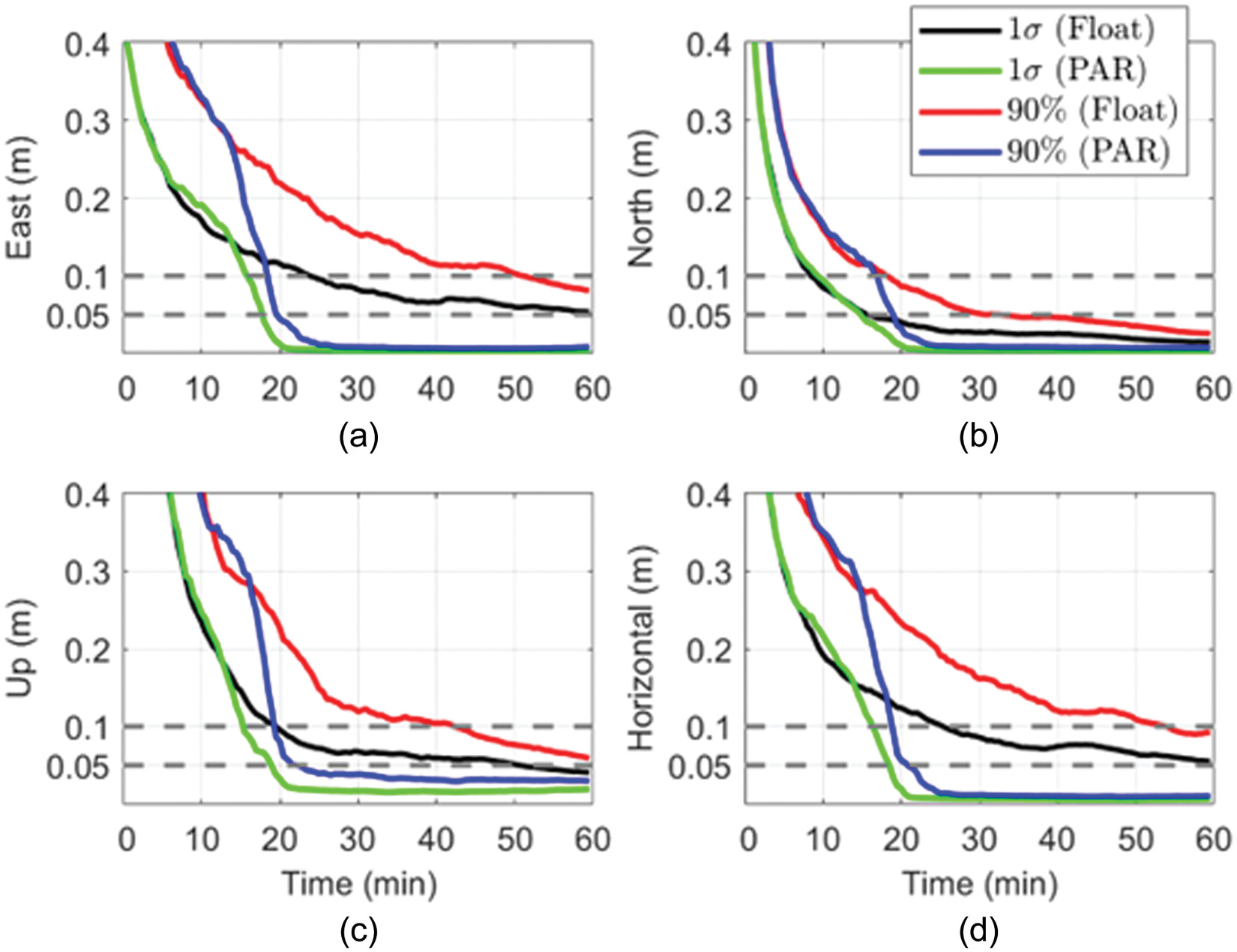
Fig. 5. The 68.27% ( $1 σ$ ) and 90% lines of the GPS-only kinematic errors in (a) the east; (b) north; (c) up; and (d) horizontal directions. The gray dashed lines mark the absolute errors of 0.1 and 0.05 m.

Fig. 6. The 68.27% ( $1 σ$ ) lines of the ambiguity-float formal standard deviations of the kinematic coordinates. G and GC indicate GPS-only and GPS/BDS-combined cases, respectively.

From Fig. 5, it can also be observed that the PAR accelerated the convergence of the user coordinates to high precision (green and blue lines in Fig. 5). With the PAR enabled, the convergence time of the 68.27% (

1 σ

) lines to 0.05 m was reduced from 51 to 19 min in the up direction and from around 60 to 18.5 min in the horizontal direction. The PAR-enabled 68.27% (

1 σ

) lines converged to 2 cm within 22.5 and 20 min in the up and horizontal directions, respectively.

The convergence to high precision was faster in the static mode benefiting from the stronger model. As illustrated in Fig. 7, compared with the kinematic mode (solid lines), the static mode (dashed-dotted lines) reduced the convergence of the PAR-enabled 68.27% (

1 σ

) lines to 0.05 m from 19 to 14.5 min in the up direction and from 18.5 to 14 min in the horizontal direction. The reduction in the convergence time of the ambiguity-float solutions was even more significant. The slow convergence behavior of the ambiguity-float kinematic horizontal coordinates [solid red line in Fig. 7(b) was primarily caused by the slow convergence behavior of the eastern coordinates (Fig. 6) due to the location of the network and the GPS satellite geometry. Using a large-scale Australian network for the UDUC PPP-RTK processing, as demonstrated by Nadarajah et al. (2018), the 50% and 75% lines of the horizontal kinematic coordinates were also worse than those in the up direction in the GPS-only ambiguity-float scenario.

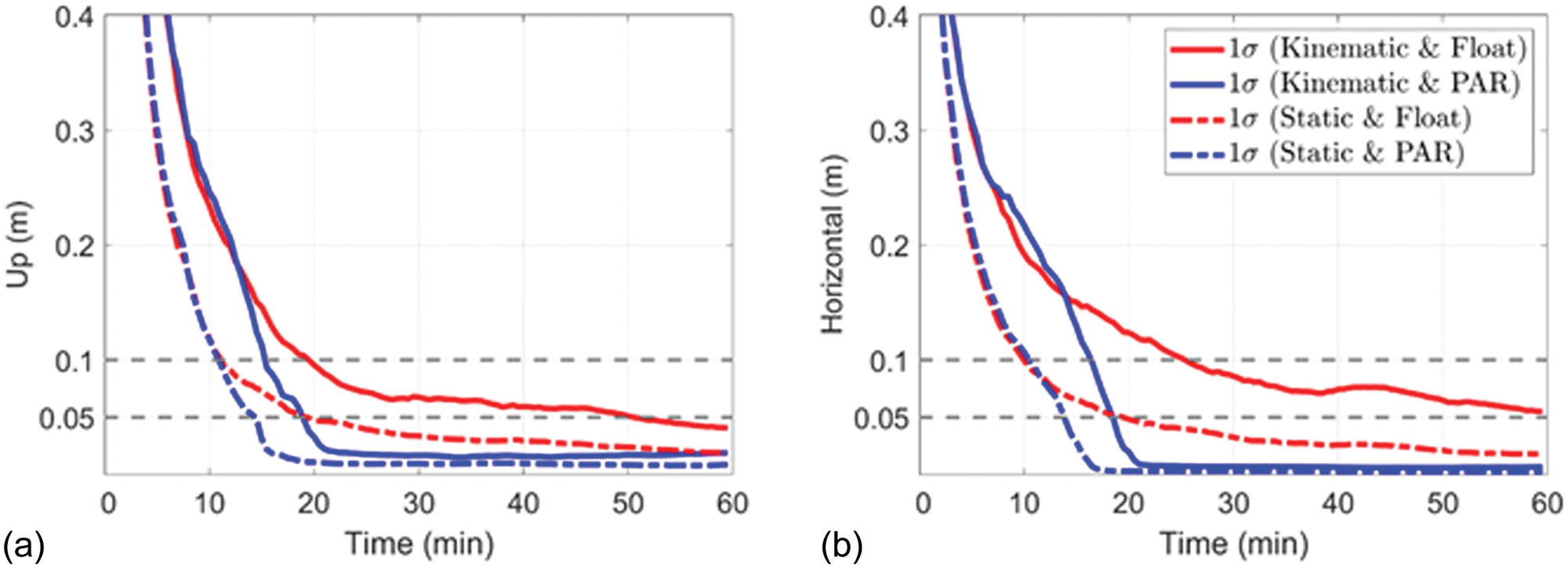
Fig. 7. The 68.27% ( $1 σ$ ) lines of the GPS-only kinematic (solid lines) and static (dash-dotted lines) errors in (a) up; and (b) horizontal directions.

Fig. 8 illustrates the convergence times of the 68.27% (

1 σ

) lines of the up and horizontal errors to 0.05 m (black and gray bars) and 0.1 m (dark and light green bars), in both the ambiguity-float case (black and dark green bars) and the PAR-enabled case (gray and light green bars). The PAR has significantly improved the convergence, especially in the GPS-only kinematic case when the model is not strong enough (top bars). Adding the BDS signals generally improved convergence. The GPS/BDS-combined PAR-enabled 68.27% (

1 σ

) lines converged to 0.05 m within 8 min in both the horizontal and up directions and in both the kinematic and static cases.

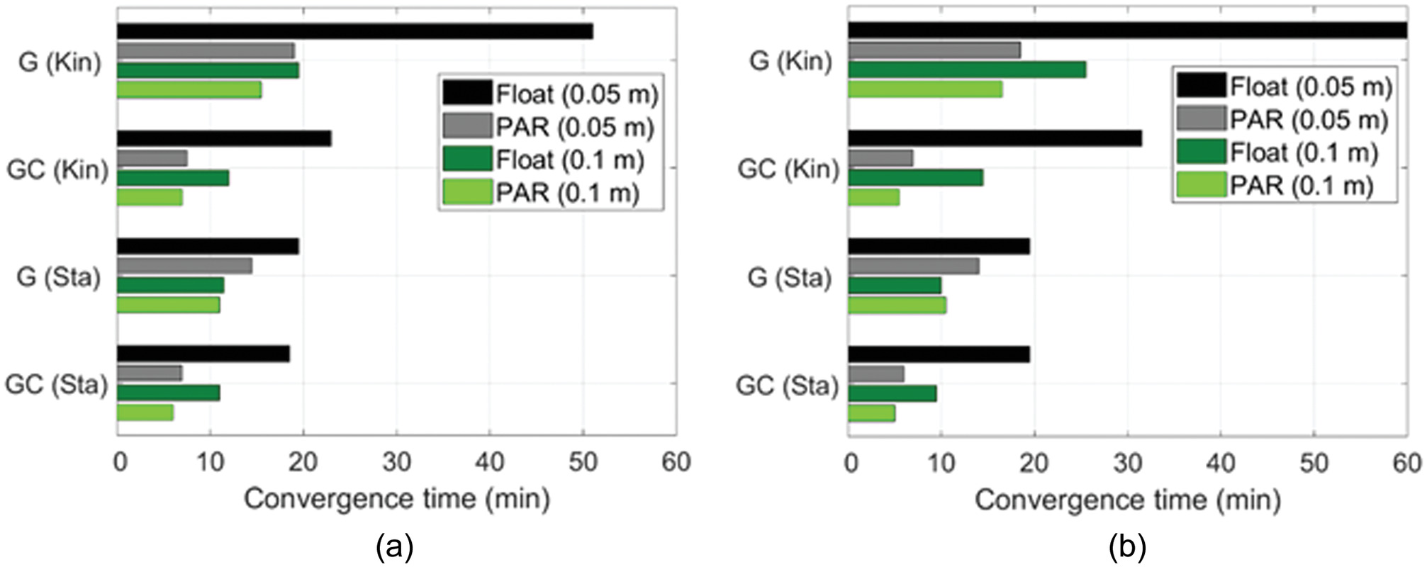
Fig. 8. Convergence times of the 68.27% ( $1 σ$ ) (a) up; and (b) horizontal errors. Kin and Sta indicate the kinematic and static modes, respectively.

The convergence times of the 68.27% (

1 σ

) and 90% lines are numerically given in Appendixes I and II, respectively. The ambiguity-float solutions required nearly, or sometimes more than, 40 min for the 90% lines to converge to 0.05 m in all cases. Even with the PAR enabled, it still took more than 20 min to allow the 90% lines of the GPS-only kinematic errors converge to 0.05 m. The convergence times are strongly dependent on the model strength, i.e., the number of satellites used, the user coordinate estimation mode, and whether the ambiguities are resolved or not. The convergence time is in general sensitive to the model strength.

GNSS and LEO Combined Solutions

In addition to the real GPS/BDS signals, the LEO satellite signals were simulated on L1 and L5 as described in the “Simulation of the LEO Satellite Signals” section. The absolute positioning errors of a representative hourly session, as an example, are illustrated in Fig. 9 in the ambiguity-float [Figs. 9(a and c)] and PAR-enabled cases [Figs. 9(b and d)] under the static mode. The solutions in Figs. 9(a and b) considered only the real GPS signals, and those in Figs. 9(c and d) were augmented by the simulated LEO signals. The LEO augmentation has reduced the convergence times in both the ambiguity-float and the PAR-enabled cases. In Figs. 9(a and b), it can be clearly observed that the PAR [Fig. 9(b)] has significantly reduced the convergence times in all directions. The differences became insignificant when augmented with LEO satellites [Figs. 9(c and d)]. With the LEO augmentation, even the ambiguity-float solutions can converge to high precision of 0.05 m in a few minutes.

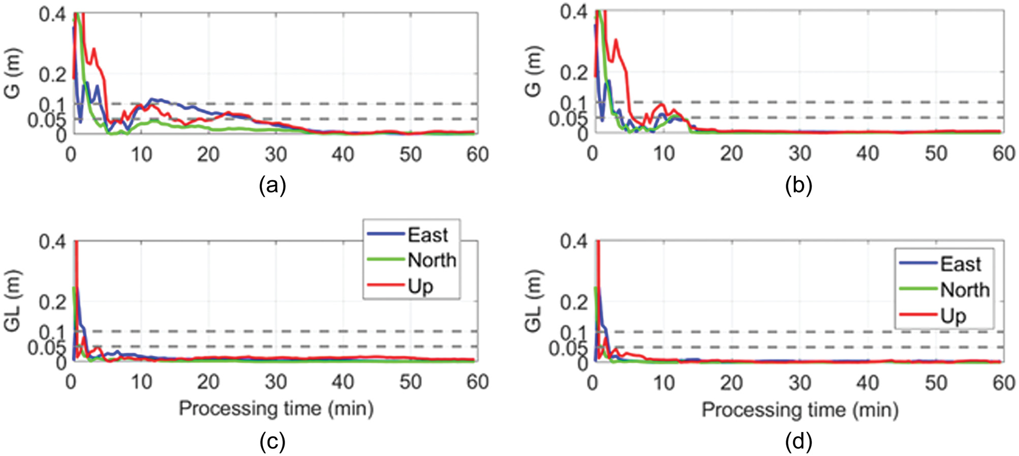
Fig. 9. (a and b) GPS-only; and (c and d) GPS/LEO combined absolute positioning errors in (a and c) ambiguity-float; and (b and d) PAR-enabled cases under the static mode. A representative hourly session of USER1 from 04:09:00 to 05:08:30 in GPST on February 1, 2022, was used for producing the plots.

The positioning solutions became worse and noisier when the user coordinates were estimated in the kinematic mode, as shown in Fig. 10. The kinematic coordinates, especially the height component, are highly correlated with the receiver clocks and ZTDs, resulting in less stable positioning solutions in general. Although the strongly shortened convergence of the LEO-augmented solutions [Figs. 10(c and d)] remain as previously, the LEO-augmented kinematic height components (red lines) were observed to be biased after the convergence, which is even more obvious in the PAR-enabled case [Fig. 10(d)].

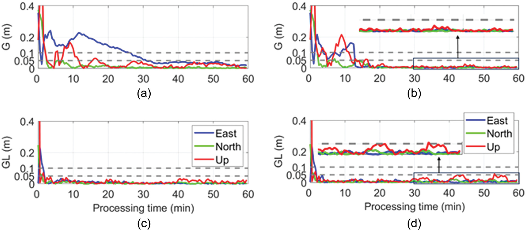
Fig. 10. (a and b) GPS-only; and (c and d) GPS/LEO combined absolute positioning errors in (a and c) ambiguity-float; and (b and d) PAR-enabled cases under the kinematic mode. A representative hourly session of USER1 from 04:09:00 to 05:08:30 in GPST on February 1, 2022, was used for producing the plots.

This can be explained as follows. As described in the “Introduction,” the LEO signals suffer from various biases in the simulations of this study that could be mismodeled. These come from, e.g., the real-time orbital errors of the low-altitude LEO satellites projected on the network and user stations, the short convergence time of the LEO-related network corrections due to their very limited visible time, and for our simulations, the biased simulated ZTDs from their true values. The biases mainly influence the height component due to its high correlation with other receiver-related parameters. The effects of the biases is more obvious when the ambiguities are fixed, which could be partially captured by the float ambiguities in the ambiguity-float case.

Compared with the GNSS satellites, the mismodeled biases of LEO satellite observations could have enlarged projections on the coordinates due to their lower heights and low elevation angles. One example is the projection of real-time orbital errors on a network of the same scale. The orbital height here plays then an important role. Also, as mentioned previously, LEO satellites mainly fly at low elevation angles. For the same satellite number, low elevation angles generally weaken the model strength and lead to a more sensitive reflection of the estimable parameters to the mismodeled biases.

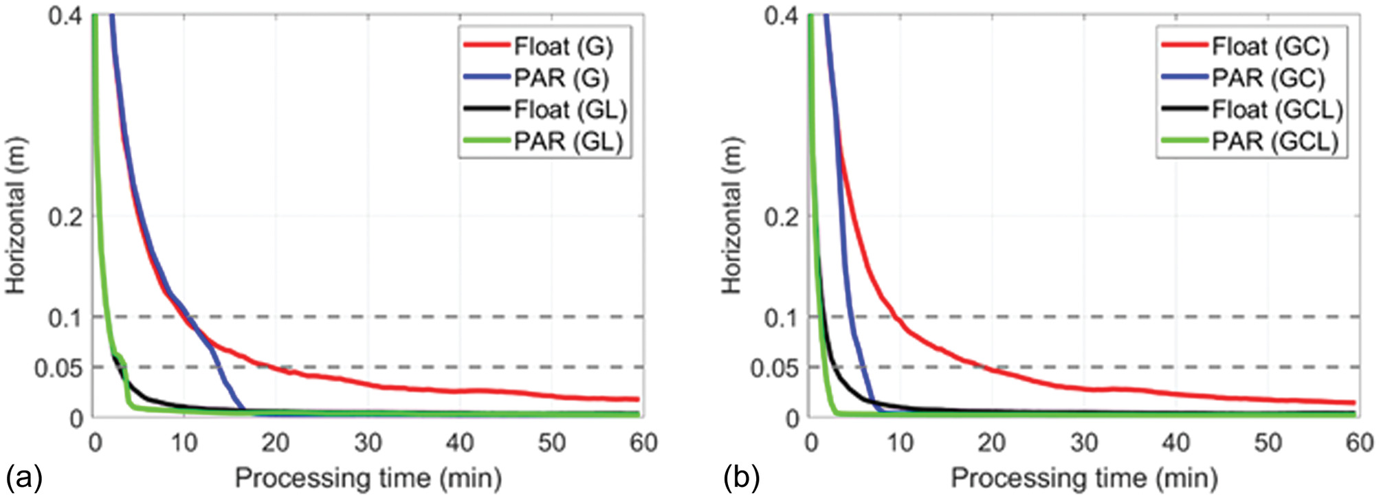
In the static mode, the 68.26% (

1 σ

) lines of the horizontal errors are illustrated in Fig. 11(a) for GPS and in Fig. 11(b) GPS/BDS-combined solutions, considering all the hourly sessions tested as in the previous subsection. With the LEO augmentation, the convergence times were significantly reduced in both the ambiguity-float and PAR-enabled cases, i.e., only 2–4 min for a convergence to 0.05 m. This applied also to the height component.

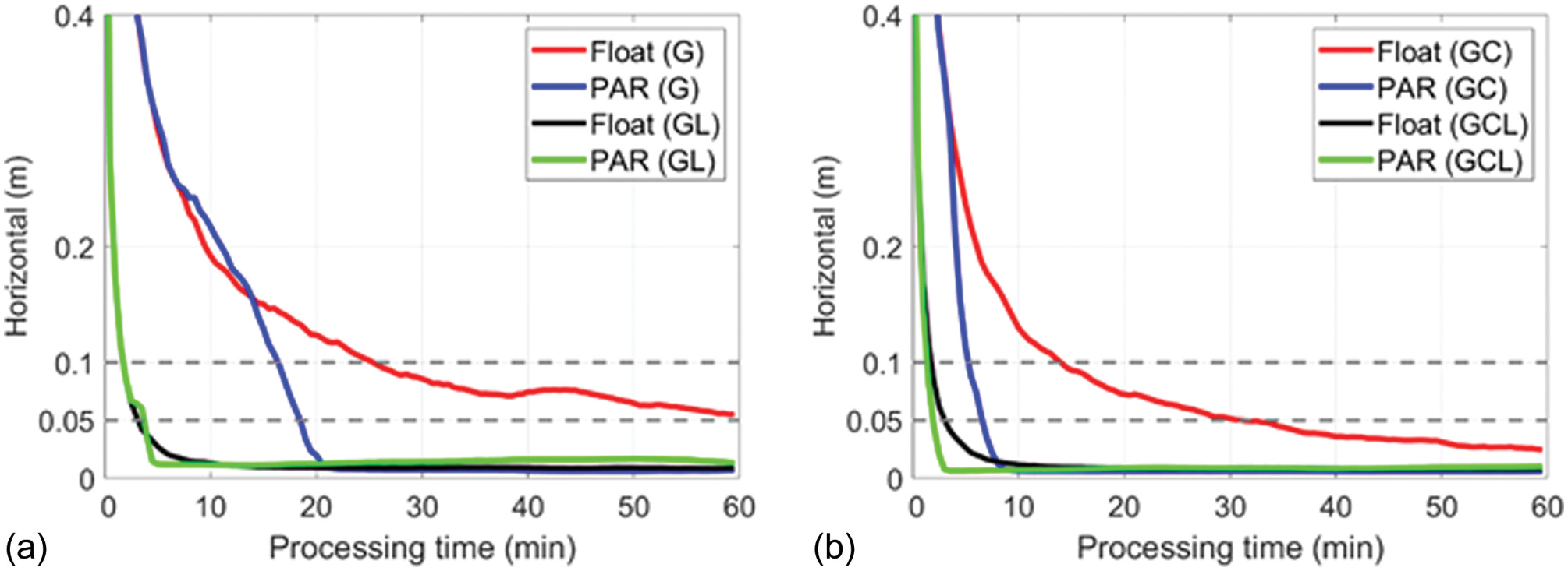
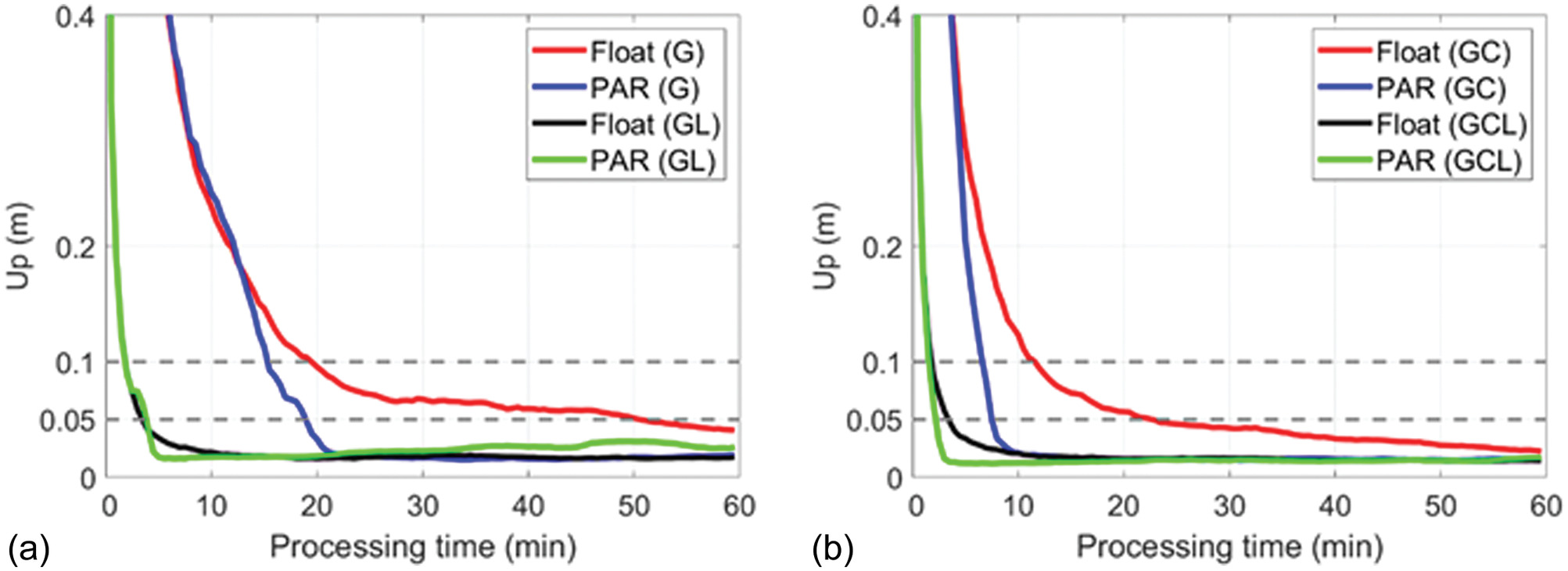
Fig. 11. The 68.27% ( $1 σ$ ) lines of the static horizontal errors for (a) GPS; and (b) GPS/BDS solutions without (G and GC) and with the LEO augmentation (GL and GCL).

When estimating the user coordinates in the kinematic mode, the sharp convergence of the solutions due to LEO augmentation remained, despite the significantly slower convergence of the GNSS-only solutions. As shown in Figs. 12 and 13, the 68.27% (

1 σ

) lines of the kinematic horizontal and height errors converged to 0.05 m within 4 min when augmented with LEO satellites. Compared with the static mode (Fig. 11), however, the PAR-enabled GPS/LEO combined solutions [green lines in Figs. 12(a) and 13(a)] are slightly biased after convergence, especially for the height component. In contrast, the corresponding ambiguity-float solutions (black lines) seem to be less disturbed by the biases after the convergence. This also corresponds to the example shown in Fig. 10.

Fig. 12. The 68.27% ( $1 σ$ ) lines of the horizontal kinematic errors for (a) GPS; and (b) GPS/BDS solutions without (G and GC) and with the LEO augmentation (GL and GCL).

Fig. 13. The 68.27% ( $1 σ$ ) lines of the kinematic height errors for (a) GPS; and (b) GPS/BDS solutions; without (G and GC) and with the LEO augmentation (GL and GCL).

The convergence times of the 68.27% (

1 σ

) lines are shown in Fig. 14 for different solution types. Those augmented with LEO satellites are marked in magenta. The convergence times, together with their corresponding improvements against the cases without the LEO augmentation, are also given in Table 3. It can be observed that the LEO augmentation significantly reduced the convergence times of the GNSS-only solutions, i.e., to within 4 min in all cases, with improvements varying from 64% to more than 94%. Having the LEO augmentation, the positioning results became less sensitive to the number of the involved GNSS satellites, the estimation mode of the user coordinates, and the choice of whether the ambiguities are to be resolved (i.e., float versus PAR).

Fig. 14. Convergence times of the 68.27% ( $1 σ$ ) lines of the (a) up; and (b) horizontal errors without and with the LEO augmentation (magenta).

Table 3. Convergence times (min) of the 68.27% (

1 σ

) lines of the GNSS with LEO-augmented positioning errors

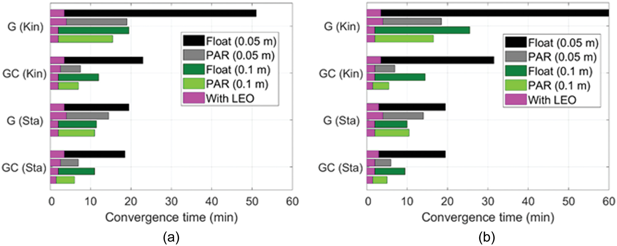
Estimation mode	Convergence time of the 68.27% lines of the float up component to $0.05 m / 0.1 m$ (min)	Convergence time of the 68.27% lines of the PAR up component to $0.05 m / 0.1 m$ (min)	Convergence time of the 68.27% lines of the horizontal up component to $0.05 m / 0.1 m$ (min)	Convergence time of the 68.27% lines of the float horizontal component to $0.05 m / 0.1 m$ (min)
GL (Kin)	3.5 $(93 %) / 2.0$ (90%)	4.0 $(79 %) / 2.0$ (87%)	$3.5 (> 94 %) / 2.0$ (92%)	4.0 $(78 %) / 2.0$ (88%)
GCL (Kin)	3.5 $(85 %) / 2.0$ (83%)	2.5 $(67 %) / 2.0$ (71%)	3.5 $(89 %) / 2.0$ (86%)	2.0 $(71 %) / 1.5$ (73%)
GL (Sta)	3.5 $(82 %) / 2.0$ (83%)	4.0 $(72 %) / 2.0$ (82%)	3.0 $(85 %) / 2.0$ (80%)	4.0 $(71 %) / 2.0$ (81%)
GCL (Sta)	3.5 $(81 %) / 2.0$ (82%)	2.5 $(64 %) / 1.5$ (75%)	3.0 $(85 %) / 2.0$ (79%)	2.0 $(67 %) / 1.5$ (70%)

Note: The percentage of improvement when compared with the GNSS-only cases is given in parentheses.

The 90% lines of the positioning errors tell more about the benefits of the LEO augmentation (Fig. 15 and Table 4). All convergence times were reduced to within 6.5 min with the LEO augmentation compared with the GNSS-only solutions, with sharp reduction in the GNSS-only ambiguity-float cases (black bars). The results suggest again that the LEO augmentation makes the convergence time of the ionosphere-float PPP-RTK solutions less sensitive to its original model strength.

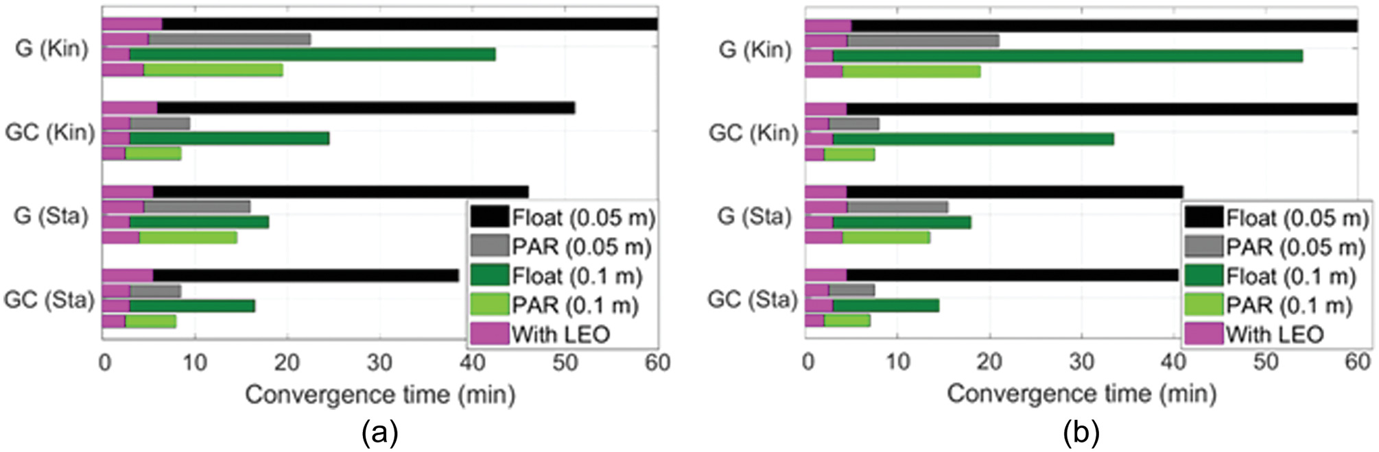
Fig. 15. Convergence times of the 90% ( $1 σ$ ) lines of the (a) up; and (b) horizontal errors without and with the LEO augmentation (magenta).

Table 4. Convergence times (in min) of the 90% lines of the LEO-augmented absolute positioning errors

Estimation mode	Convergence time of the 90% lines of the float up component to $0.05 m / 0.1 m$ (min)	Convergence time of the 90% lines of the PAR up component to $0.05 m / 0.1 m$ (min)	Convergence time of the 90% lines of the float horizontal component to $0.05 m / 0.1 m$ (min)	Convergence time of the 90% lines of the PAR horizontal component to $0.05 m / 0.1 m$ (min)
GL (Kin)	6.5 $(> 89 %) / 3.0$ (93%)	5.0 $(78 %) / 4.5$ (77%)	5.0 $(> 92 %) / 3.0$ (94%)	4.5 $(79 %) / 4.0$ (79%)
GCL (Kin)	6.0 $(88 %) / 3.0$ (88%)	3.0 $(68 %) / 2.5$ (71%)	4.5 $(> 93 %) / 3.0$ (91%)	2.5 $(69 %) / 2.0$ (73%)
GL (Sta)	5.5 $(88 %) / 3.0$ (83%)	4.5 $(72 %) / 4.0$ (72%)	4.5 $(89 %) / 3.0$ (83%)	4.5 $(71 %) / 4.0$ (70%)
GCL (Sta)	5.5 $(86 %) / 3.0$ (82%)	3.0 $(65 %) / 2.5$ (69%)	4.5 $(89 %) / 3.0$ (79%)	2.5 $(67 %) / 2.0$ (71%)

Note: The percentage of improvement compared with the GNSS-only cases is given in parentheses.

Conclusions

The ionosphere-float PPP-RTK positioning technique is often applied in large-scale networks. In such a case, the ionospheric corrections are not attempted to be provided to users for interpolation, which hampers fast IAR and solution convergence on the user side. The augmentation by LEO satellites can bridge this shortcoming thanks to their fast speed and the resulting rapid geometry change. In this study, using a network with a scale of thousands of kilometers, real GPS and BDS dual-frequency observations, and simulated LEO observations on L1/L5 based on the CentiSpace constellation were used to test the convergence times of the PPP-RTK solutions under both the kinematic and static modes and in both the ambiguity-float and PAR-enabled cases.

The results suggest that the convergence times of the GNSS-only solutions are sensitive to the constellation involved, the estimation mode of the users, and whether ambiguities are resolved or kept float. The PAR decreased the convergence times of the ambiguity-float solutions, the GPS/BDS-combined results outperformed the GPS-only ones, and the static user results behaved better than those under the kinematic mode. Still, without LEO augmentation, long convergence times are required in certain circumstances. It took nearly, or sometimes more than, 40 min to enable the 90% lines of the ambiguity-float kinematic positioning errors to converge to 0.05 m in both the horizontal and up directions under both the static and kinematic modes. Even with the PAR enabled, the convergence of the 90% lines of the GPS-only kinematic solutions took more than 20 min.

With the LEO augmentation of GNSS observations, the convergence times of all-cases of PPP-RTK solutions were significantly reduced, i.e., to within 4.5 min for the 68.27% (

1 σ

) lines and within 6.5 min for the 90% lines. This applies to both the GPS-only and GPS/BDS-combined scenarios, both the ambiguity-float and PAR-enabled cases, and both the static and kinematic estimation modes. The LEO augmentation made the solution convergences less sensitive to the aforementioned different conditions. With the PAR-enabled, the GPS/BDS/LEO combined 90% lines can converge to 0.05 m within 2.5 min in the horizontal direction and within 3 min in the up direction under both the kinematic and static modes.

Although with a notably shortened convergence time, it was observed in this study that after the convergence or ambiguity resolution, the mismodeled biases could have enlarged influences on the coordinates in the LEO-augmented scenario due to the low orbital heights and elevation angles of the LEO satellites. This requires further research and validation when real LEO navigation signals become available.

Appendix I. Convergence Times of the 68.27% ( $1 σ$ ) Lines of the Positioning Errors in GPS-Only and GPS/BDS Combined Scenarios

Estimation mode	Convergence time of the 68.27% lines of the float up component to $0.05 m / 0.1 m$ (min)	Convergence time of the 68.27% lines of the PAR up component to $0.05 m / 0.1 m$ (min)	Convergence time of the 68.27% lines of the float horizontal component to $0.05 m / 0.1 m$ (min)	Convergence time of the 68.27% lines of the PAR horizontal component to $0.05 m / 0.1 m$ (min)
G (Kin)	$51.0 / 19.5$	$19.0 / 15.5$	$> 60.0 / 25.5$	$18.5 / 16.5$
GC (Kin)	$23.0 / 12.0$	$7.5 / 7.0$	$31.5 / 14.5$	$7.0 / 5.5$
G (Sta)	$19.5 / 11.5$	$14.5 / 11.0$	$19.5 / 10.0$	$14.0 / 10.5$
GC (Sta)	$18.5 / 11.0$	$7.0 / 6.0$	$19.5 / 9.5$	$6.0 / 5.0$

Note: G = GPS; C = BDS; Kin = kinematic mode; and Sta = static modes.

Appendix II. Convergence Times of the 90% Lines of the Positioning Errors in GPS-Only and GPS/BDS-Combined Scenarios

Estimation mode	Convergence time of the 90% lines of the float up component to $0.05 m / 0.1 m$ (min)	Convergence time of the 90% lines of the PAR up component to $0.05 m / 0.1 m$ (min)	Convergence time of the 90% lines of the float horizontal component to $0.05 m / 0.1 m$ (min)	Convergence time of the 90% lines of the PAR horizontal component to $0.05 m / 0.1 m$ (min)
G (Kin)	$> 60.0 / 42.5$	$22.5 / 19.5$	$> 60.0 / 54.0$	$21.0 / 19.0$
GC (Kin)	$51.0 / 24.5$	$9.5 / 8.5$	$> 60.0 / 33.5$	$8.0 / 7.5$
G (Sta)	$46.0 / 18.0$	$16.0 / 14.5$	$41.0 / 18.0$	$15.5 / 13.5$
GC (Sta)	$38.5 / 16.5$	$8.5 / 8.0$	$40.5 / 14.5$	$7.5 / 7.0$

Data Availability Statement

Some data, models, or code generated or used during the study are available in a repository or online in accordance with funder data retention policies. This includes the CNES real-time GNSS products available at http://www.ppp-wizard.net/products/REAL_TIME/. Some data, models, or code generated or used during the study are available from the corresponding author by reasonable request. This includes the station observation data, which can be made available upon reasonable request and with the permission of the BDS High-precision Spatiotemporal Service Characteristic Science Database.

Acknowledgments

This research is funded by the National Time Service Center, Chinese Academy of Sciences (CAS) (No. E167SC14), the National Natural Science Foundation of China (No. 12073034), the CAS “Light of West China” Program (XAB2021YN25), Shaanxi Province Key R&D Program Project (2022KW-29), and the Australian Research Council—discovery project (No. DP 190102444). We acknowledge the support of the BDS High-Precision Spatiotemporal Service Characteristic Science Database, the international GNSS monitoring and assessment system (iGMAS) at the National Time Service Center, and the National Space Science Data Center, National Science & Technology Infrastructure of China (http://www.nssdc.ac.cn).

References

Baarda, W. 1981. “S-transformations and criterion matrices.” In Publications on geodesy. 2nd ed. Delft, Netherlands: Netherlands Geodetic Commission.

Google Scholar

Cakaj, S., B. Kamo, A. Lala, and A. Rakipi. 2014. “The coverage analysis for low earth orbiting satellites at low elevation.” Int. J. Adv. Comput. Sci. Appl. 5 (Jun): 6. https://doi.org/10.14569/IJACSA.2014.050602.

Google Scholar

Collins, P. 2008. “Isolating and estimating undifferenced GPS integer ambiguities.” In Proc., 2008 National Technical Meeting of the Institute of navigation, 720–732. Manassas, VA: Institute of Navigation.

Google Scholar

Ge, H., B. Li, M. Ge, N. Zang, L. Nie, Y. Shen, and H. Schuh. 2018. “Initial assessment of precise point positioning with LEO enhanced global navigation satellite systems (LeGNSS).” Remote Sens. 10 (7): 984. https://doi.org/10.3390/rs10070984.

Google Scholar

Ge, M., G. Gendt, M. Rothacher, C. Shi, and J. Liu. 2008. “Resolution of GPS carrier phase ambiguities in precise point positioning (PPP) with daily observations.” J. Geod. 82 (7): 389–399. https://doi.org/10.1007/s00190-007-0187-4.

Google Scholar

Geng, J., X. Meng, A. H. Dodson, M. Ge, and F. N. Teferle. 2010. “Rapid re-convergences to ambiguity-fixed solutions in precise point positioning.” J. Geod. 84 (12): 705–714. https://doi.org/10.1007/s00190-010-0404-4.

Google Scholar

Hassan, T., A. El-Mowafy, and K. Wang. 2020. “A review of system integration and current integrity monitoring methods for positioning in intelligent transport systems.” IET Intel. Transport Syst. 15 (1): 43–60. https://doi.org/10.1049/itr2.12003.

Google Scholar

Hauschild, A., J. Tegedor, O. Montenbruck, H. Visser, and M. Markgraf. 2016. “Precise onboard orbit determination for LEO satellites with real-time orbit and clock corrections.” In Proc., 29th Int. Technical Meeting of the Satellite Division of the Institute of Navigation (ION GNSS+ 2016), 3715–3723. Portland, OR: Institute of Navigation.

Google Scholar

Hong, J., R. Tu, P. Zhang, J. Han, L. Fan, S. Wang, and X. Lu. 2023. “GNSS rapid precise point positioning enhanced by low Earth orbit satellites.” Satell. Navig. 4 (1): 11. https://doi.org/10.1186/s43020-023-00100-x.

Google Scholar

Ifadis, I. 1986. The atmospheric delay of radio waves: Modeling the elevation dependence on a global scale. Göteborg, Sweden: Chalmers Univ. of Technology.

Google Scholar

Kazmierski, K., K. Sosnica, and T. Hadas. 2018. “Quality assessment of multi-GNSS orbits and clocks for real-time precise point positioning.” GPS Solutions 22 (Jan): 11. https://doi.org/10.1007/s10291-017-0678-6.

Google Scholar

Li, Q., W. Yao, R. Tu, Y. Du, and M. Liu. 2023. “Performance assessment of multi-GNSS PPP ambiguity resolution with LEO-augmentation.” Remote Sens. 15 (12): 2958. https://doi.org/10.3390/rs15122958.

Google Scholar

Li, X., X. Li, F. Ma, Y. Yuan, K. Zhang, F. Zhou, and X. Zhang. 2019. “Improved PPP ambiguity resolution with the assistance of multiple LEO constellations and signals.” Remote Sens. 11 (4): 408. https://doi.org/10.3390/rs11040408.

Google Scholar

Li, X., F. Ma, X. Li, H. Lv, L. Bian, Z. Jiang, and X. Zhang. 2018. “LEO constellation-augmented multi-GNSS for rapid PPP convergence.” J. Geod. 93 (Aug): 749–764. https://doi.org/10.1007/s00190-018-1195-2.

Google Scholar

Lv, Y., T. Geng, Q. Zhao, X. Xie, F. Zhang, and X. Wang. 2020. “Evaluation of BDS-3 orbit determination strategies using ground-tracking and inter-satellite link observation.” Remote Sens. 12 (16): 2647. https://doi.org/10.3390/rs12162647.

Google Scholar

Montenbruck, O., and E. Gill. 2000. “Around the world in a hundred minutes.” In Satellite orbits. 1st ed., 1–13. Berlin: Springer.

Crossref

Google Scholar

Montenbruck, O., F. Kunzi, and A. Hauschild. 2021. “Performance assessment of GNSS–based real–time navigation for the Sentinel–6 spacecraft.” GPS Solutions 26 (Jun): 12. https://doi.org/10.1007/s10291-021-01198-9.

Google Scholar

Nadarajah, N., A. Khodabandeh, K. Wang, M. Choudhury, and P. J. G. Teunissen. 2018. “Multi-GNSS PPP-RTK: From large- to small-scale networks.” Sensors 18 (4): 1078. https://doi.org/10.3390/s18041078.

Google Scholar

Nardo, A., B. Li, and P. J. G. Teunissen. 2016. “Partial ambiguity resolution for ground and space-based applications in a GPS + Galileo scenario: A simulation study.” Adv. Space Res. 57 (1): 30–45. https://doi.org/10.1016/j.asr.2015.09.002.

Google Scholar

Odijk, D., A. Khodabandeh, N. Nadarajah, M. Choudhury, B. Zhang, W. Li, and P. J. G. Teunissen. 2016. “PPP-RTK by means of S-system theory: Australian network and user demonstration.” J. Spatial Sci. 62 (1): 3–27. https://doi.org/10.1080/14498596.2016.1261373.

Google Scholar

Odijk, D., P. Teunissen, and B. Zhang. 2012. “Single-frequency integer ambiguity resolution enabled GPS precise point positioning.” J. Surv. Eng. 138 (4): 193–202. https://doi.org/10.1061/(ASCE)SU.1943-5428.0000085.

Google Scholar

Odijk, D., B. Zhang, A. Khodabandeh, R. Odolinski, and P. J. G. Teunissen. 2015. “On the estimability of parameters in undifferenced, uncombined GNSS network and PPPRTK user models by means of S-system theory.” J. Geod. 90 (1): 15–44. https://doi.org/10.1007/s00190-015-0854-9.

Google Scholar

Perez, R. 1998. “Introduction to satellite systems and personal wireless communications.” In Wireless communications design handbook, 1–30. London: Academic Press. https://doi.org/10.1016/S1874-6101(99)80014-3.

Google Scholar

Psychas, D., and S. Verhagen. 2020. “Real-time PPP-RTK performance analysis using ionospheric corrections from multi-scale network configurations.” Sensors 20 (11): 3012. https://doi.org/10.3390/s20113012.

Google Scholar

Pullen, S., Y. S. Park, and P. Enge. 2009. “Impact and mitigation of ionospheric anomalies on ground-based augmentation of GNSS.” Radio Sci. 44 (1): RS0A21. https://doi.org/10.1029/2008RS004084.

Google Scholar

Rebischung, P., and R. Schmid. 2016. “IGS14/igs14.atx: A new framework for the IGS products.” In Proc., Fall Meeting 2016. San Francisco: American Geophysical Union.

Google Scholar

Teunissen, P. J. G. 1985. “Zero order design: Generalized inverses, adjustment, the datum problem and S-transformations.” In Optimization and design of geodetic networks, 11–55. Berlin: Springer. https://doi.org/10.1007/978-3-642-70659-2_3.

Google Scholar

Teunissen, P. J. G. 1993. “Least-squares estimation of the integer GPS ambiguities. Invited lecture, Section IV theory and methodology.” In Proc., IAG General Meeting, Beijing, China. Masala, Finland: International Association of Geodesy.

Google Scholar

Teunissen, P. J. G. 1995. “The least-squares ambiguity decorrelation adjustment: A method for fast GPS integer ambiguity estimation.” J. Geod. 70 (1–2): 65–82. https://doi.org/10.1007/BF00863419.

Google Scholar

Teunissen, P. J. G., and A. Khodabandeh. 2015. “Review and principles of PPP-RTK methods.” J. Geod. 89 (3): 217–240. https://doi.org/10.1007/s00190-014-0771-3.

Google Scholar

Teunissen, P. J. G., D. Odijk, and B. Zhang. 2010. “PPP-RTK: Results of CORS network-based PPP with integer ambiguity resolution.” J. Aeronaut. Astronaut. Aviat. 42 (4): 223–230.

Google Scholar

Walker, J. G. 1984. “Satellite constellations.” J. Br. Interplanet. Soc. 37 (Dec): 559–571.

Google Scholar

Wang, K., A. El-Mowafy, W. Wang, L. Yang, and X. Yang. 2022a. “Integrity monitoring of PPP-RTK positioning; Part II: LEO augmentation.” Remote Sens. 14 (7): 1599. https://doi.org/10.3390/rs14071599.

Google Scholar

Wang, K., B. Sun, W. Qin, X. Mi, A. El-Mowafy, and X. Yang. 2022b. “A method of real-time long-baseline time transfer based on the PPP-RTK.” Adv. Space Res. 71 (3): 1363–1376. https://doi.org/10.1016/j.asr.2022.10.062.

Google Scholar

Wu, J., S. Wu, G. Hajj, W. Bertiguer, and S. Lichten. 1993. “Effects of antenna orientation on GPS carrier phase measurements.” Manuscr. Geod. 18 (Jun): 91–98.

Google Scholar

Wübbena, G., M. Schmitz, and A. Bagge. 2005. “PPP-RTK: Precise point positioning using state-space representation in RTK networks.” In Proc., 18th Int. Technical Meeting of the Satellite Division of the Institute of Navigation (ION GNSS 2005), 2584–2594. Manassas, VA: Institute of Navigation.

Google Scholar

Yang, L. 2019. “The CentiSpace-1: A LEO satellite-based augmentation system.” In Proc., 14th Meeting of the Int. Committee on Global Navigation Satellite Systems, Bengaluru, India. Vienna, Austria: United Nations Office for Outer Space Affairs.

Google Scholar

Zhang, B., P. Hou, and R. Odolinski. 2022. “PPP-RTK: From common-view to all-in-view GNSS networks.” J. Geod. 96 (Jun): 102. https://doi.org/10.1007/s00190-022-01693-y.

Google Scholar

Zhao, Q., S. Pan, C. Gao, W. Gao, and Y. Xia. 2020. “BDS/GPS/LEO triple-frequency uncombined precise point positioning and its performance in harsh environments.” Measurement 151 (Jun): 107216. https://doi.org/10.1016/j.measurement.2019.107216.

Google Scholar

Information & Authors

Information

Published In

Journal of Surveying Engineering

Volume 150 • Issue 2 • May 2024

Copyright

This work is made available under the terms of the Creative Commons Attribution 4.0 International license, https://creativecommons.org/licenses/by/4.0/.

History

Received: Oct 11, 2022

Accepted: Oct 11, 2023

Published online: Jan 4, 2024

Published in print: May 1, 2024

Discussion open until: Jun 4, 2024

Authors

Affiliations

Kan Wang https://orcid.org/0000-0001-5688-6937 [email protected]

Professor, National Time Service Center, Chinese Academy of Sciences, Xi’an 710600, China; Univ. of Chinese Academy of Sciences, Beijing 100049, China; Key Laboratory of Time Reference and Applications, Chinese Academy of Sciences, Xi’an 710600, China (corresponding author). ORCID: https://orcid.org/0000-0001-5688-6937. Email: [email protected]

View all articles by this author

Ahmed El-Mowafy https://orcid.org/0000-0001-7060-4123 [email protected]

Professor, School of Earth and Planetary Sciences, Curtin Univ., Perth, WA 6845, Australia. ORCID: https://orcid.org/0000-0001-7060-4123. Email: [email protected]

View all articles by this author

Fang Cheng [email protected]

Professor, National Time Service Center, Chinese Academy of Sciences, Xi’an 710600, China; Univ. of Chinese Academy of Sciences, Beijing 100049, China; Key Laboratory of Time Reference and Applications, Chinese Academy of Sciences, Xi’an 710600, China. Email: [email protected]

View all articles by this author

Xuhai Yang [email protected]

Professor, National Time Service Center, Chinese Academy of Sciences, Xi’an 710600, China; Univ. of Chinese Academy of Sciences, Beijing 100049, China; Key Laboratory of Time Reference and Applications, Chinese Academy of Sciences, Xi’an 710600, China. Email: [email protected]

View all articles by this author

Metrics & Citations

Metrics

Citations

Download citation

If you have the appropriate software installed, you can download article citation data to the citation manager of your choice. Simply select your manager software from the list below and click Download.

LEO Augmentation in Large-Scale Ionosphere-Float PPP-RTK Positioning

Abstract

Introduction

Processing Strategy

Network Model

User Model

Data Processing

GNSS Real Data

Simulation of the LEO Satellite Signals

Test Results

GNSS-Based Real-Data Solutions without LEO Augmentation

GNSS and LEO Combined Solutions

Conclusions

Appendix I. Convergence Times of the 68.27% ( $1 σ$ ) Lines of the Positioning Errors in GPS-Only and GPS/BDS Combined Scenarios

Appendix II. Convergence Times of the 90% Lines of the Positioning Errors in GPS-Only and GPS/BDS-Combined Scenarios

Data Availability Statement

Acknowledgments

References

Information & Authors

Information

Published In

Copyright

History

Authors

Affiliations

Metrics & Citations

Metrics

Citations

Download citation

View Options

Media

Figures

Other

Tables

NEXT ARTICLE

Verify Phone

Congrats!

Abstract

Introduction

Processing Strategy

Network Model

User Model

Data Processing

GNSS Real Data

Simulation of the LEO Satellite Signals

Test Results

GNSS-Based Real-Data Solutions without LEO Augmentation

GNSS and LEO Combined Solutions

Conclusions

Appendix I. Convergence Times of the 68.27% (1σ) Lines of the Positioning Errors in GPS-Only and GPS/BDS Combined Scenarios

Appendix II. Convergence Times of the 90% Lines of the Positioning Errors in GPS-Only and GPS/BDS-Combined Scenarios

Data Availability Statement

Acknowledgments

References

Information

Published In

Copyright

History

Authors

Affiliations

Metrics

Citations

Download citation

Figures

Other

Share

Copy the content Link

Share with email

Share

Request Username

Create a new account

Change Password

Password Changed Successfully

Verify Phone

Congrats!

Appendix I. Convergence Times of the 68.27% ( $1 σ$ ) Lines of the Positioning Errors in GPS-Only and GPS/BDS Combined Scenarios