Seismic Response Comparison of Full-Scale Moment-Resisting Timber Frame and Joint Test Result
Publication: Journal of Structural Engineering
Volume 149, Issue 7
Abstract
This paper presents the seismic performance of the moment-resisting timber frame (MRTF). In Japanese urban areas, there are many urban small houses, and it is difficult to design a wooden building to ensure both the seismic performance and the comfortable plan that effectively makes use of small and constrained sites, and it also lacks flexibility in the design. Therefore, expectations are rising for high performance of MRTF using residential members. In this study, to clarify the seismic performance and the dynamic behavior under the heavy seismic wave, we conducted a full-shaking table test of the 2-story MRTF composed of residential members with short sides. The structure was designed by the allowable stress design (ASD) to resist 1.5 times the earthquake ground motion required in Japanese Building Standard Law (BSL) and linear analysis under frequent loading conditions (snow, wind, and earthquake events corresponding to a return period of approximately 50 years), and the unidirectional full-scale shaking table tests were conducted. The structure did not collapse up to a peak ground acceleration of and experienced of maximum interstory drift. This indicates that an MRTF designed by the method can secure the seismic performance for a large earthquake. The time-response analysis was also conducted based on the joint tests, but the stiffness of the analytical result is little lower than the experimental result. Then, we tried the parameter identification using quality engineering to reproduce the experimental behavior. The results indicated that the moment resistance of the joint was higher because of the stressed-skin effect of the floor.
Introduction
Japan is an earthquake-prone country, and many wooden houses have been severely damaged by earthquakes. Most houses in Japan are made of a wooden frame construction with shear walls and the seismic performance of those houses depends mostly on the amount of shear walls. However, especially in Japan, it is difficult to install enough shear walls in both directions, especially for a narrow site in an urban area and ensure both the seismic performance and the comfortable plan that effectively makes use of the site, and it also lacks flexibility in the design. For example, houses with garages, parking areas, and stores are difficult to design because of the difficulty in arranging shear walls. In fact, such houses were severely damaged in the Osaka-Kobe Earthquake of 1995.
To design such buildings, the moment-resisting timber frame (MRTF) is suitable compared with shear walls. There are great expectations for MRTF, and many studies have been conducted to clarify the seismic performance. For example, Bouchaïr et al. (2007) conducted experiment and numerical analysis of a moment-resisting joint, and the damage was analyzed. Heiduschke et al. (2009) conducted a small- and full-scale shaking table test of a laminated timber frame. The objective was to investigate the dynamic behavior, and the effect of the reinforcement of the moment beam–column connection. The study clarified that improvement of the moment joint is a viable option to improve the moment-resisting joint. Kasal et al. (2014) conducted the shaking table test of the MRTF with rigid connections. The structure showed high stiffness, but the brittle failure due to stress concentration was confirmed after the heavy seismic waves. The main seismic element in MRTF is moment resistance of the joint, so the study for joints was conducted. Solario et al. (2017) conducted an experiment and analysis of a timber connection and they validated the analysis model. Guo and Shu (2019) investigated the moment resistance of a bolted connection. They conducted experiments and analysis to clarify the behavior and suggested a theoretical evaluation method. These studies about joints will lead to accurate prediction of the MRTF. As stated, the MRTF was studied by some experiments and numerical analysis in places outside of Japan. However, the target structures in these studies were mainly large buildings. In Japan, the MRTF with large dimensional lumber was also studied, and some buildings were constructed based on those studies (Komatsu 2016).
On the other hand, for the residential buildings, some Japanese home manufacturers have developed the strong moment-resisting joint (e.g., Hiyama et al. 2014; Ohira et al. 2014). In addition, full-scale shaking table tests were conducted to clarify the performance. Nasu et al. (2007) conducted a full-shaking table test of a 3-story MRTF and numerical analysis and confirmed the seismic performance. Nakagawa et al. (2009) investigated the seismic performance of three types of wooden structure: MRTF, a conventional wooden house with shear wall, and a composite structure consisting of the moment-resisting frame with shear walls. They clarified that the energy dissipation of the MRTF was higher than that of the structure with shear walls. Although these studies were about the full-scale shaking table tests, the experiments of joints were also rightfully conducted before the shaking tests.
As aforementioned, Japan is an earthquake-prone country. Japanese seismic design requires the structure not to be damaged under frequent loading conditions (snow, wind, and earthquake events corresponding to a return period of approximately 50 years), and that the building will not collapse in the event of the largest earthquake ever recorded. For small-size buildings, such as residential buildings, the structural analysis to ensure nondamage against a moderate earthquake and the structural analysis to resist against a major earthquake can be omitted. On the other hand, in order to minimize damage under earthquakes, the aforementioned minimum standard of 1.5 times the earthquake ground motion required in Japanese Building Standard Law (BSL) has recently been used in the design of some residential houses in Japan. In this design, the earthquake ground motion required in BSL is based on the spectral accelerations and those will be multiplied by 1.5. In the severe earthquake zone of the 2016 Kumamoto earthquake, some houses built to the minimum standard were close to collapsing, but those built to resist 1.5 times the standard, which is called the “Earthquake Resistance Grade 3,” were able to continue to live in their homes with only minor repairs (e.g., AIJ 2017; Sumida et al. 2019). Thus, today, there is an increasing demand for housing built with higher seismic performance such as the Earthquake Resistance Grade 3.
Shaking table tests are very expensive, and it is difficult to confirm the damage condition using the design level as a parameter and to conduct tests for several different types of seismic motions and many plans. Therefore, a parameter study needs to be conducted by using an analytical approach. If the numerical analysis is conducted by determining the spring parameters of the analytical model based on elemental experiments, the deformation of the tests often will be overestimated (e.g., Noda et al. 2019). The cause of this overestimation, or underestimation of the structural model, is expected to be the combined effects of nonstructural members and materials. Isoda et al. (2021) clarified that the results of full-scale experiments underestimated the analytical results even if all elements were taken into account.
In this study, full-scale shaking table tests and numerical analysis were conducted to confirm the seismic performance of the MRTF designed to resist 1.5 times the moderate earthquake. The main objective of these tests was to determine the response deformation and the extent of damage to moderate, large, and extreme earthquakes. In order to accurately simulate various seismic motions, more accurate parameters were estimated by data assimilation, which will contribute to future studies for the numerical analysis. The data assimilation is a mathematical discipline seeking analytical parameters to agree with observations (Kalnay 2003). One of the objectives of this study was to compare the parameters obtained with those defined from elemental experiments, and to mention the causes of the differences in the parameters. In the structural engineering field, it is actively being studied as a theory for identifying the modal characteristics and analytical parameters of structures by observing the response during an earthquake and using microtremor measurement (e.g., Housner et al. 1997). In this study, the used parameter identification method is called data assimilation from the viewpoint of changing the analytical parameters such as rigidity and strength. This study targets the detailed analysis model to simulate the local behavior such as the joint rotation, and the parameters to reproduce the test results were studied. In this detailed analysis model, it is not possible to obtain an explicit solution, and the skeleton curve of the element parameters is fluctuated by trial and error to obtain the optimum solution. Although the amount of calculation is enormous, we have succeeded in reducing it by using quality engineering, and we also report on the calculation process.
Outline of the Full-Shaking Table Test
Design Concept
In Japanese seismic code, two-phase design has usually been required since 1981 (MLIT 2008). The first-phase design is based on allowable stress design (ASD), and how the structure responds elastically during a moderate earthquake. The second-phase design is to ensure the life safety against a severe earthquake, which is considered the maximum earthquake in limit state design (LSD). For 2-story residential houses, a prescribed amount of shear wall per square meter is required [Notification 1100 of the Ministry of Construction (2007)] because most houses in Japan are made of a wooden frame construction with shear walls and the seismic performance depends mostly on the amount of shear walls. On the other hand, for a wooden house with moment-resisting connections that are main seismic elements, calculation is required as subsequently explained. The small-size and low-rise structure dealt with in this study has to only obey to ASD not LSD in law. From the trend of performance-based seismic design, it is a key issue to prevent the collapse against an expected earthquake. The objective of the first-phase design is preventing structural damage under frequent loading conditions. Concretely, the stresses at structural members were calculated by a linear elastic analysis under the seismic forces that are within their allowable stress.
The design shear force of each story is calculated using Eq. (1) according to the Japanese standardwhere is the base shear coefficient; is the vertical distribution factor; is the weight of story; seismic zone factor and vibration characteristic factor were set as 1.0; is the natural period (for timber structure, , where H is the total height); is the the number of stories above base; and is the story number.
(1a)
(1b)
(1c)
While is usually set as 0.2 for ASD, to design the specimen with the Earthquake Resistance Grade 3 based on ASD, we defined is in this study. The analysis model as described in the next section was used and the design was carried out according to the following:
1.
When the design shear force, which is equivalent to a moderate earthquake, is loaded to the structure, stresses occurring in members and joints shall be less than the allowable stress.
2.
Stiffness should be secured so that the interstory deformation angle during a moderate earthquake is within at least .
The allowable value for members is defined of two-thirds of the nominal strength. The capacity of the joint will be assigned the 95% lower limit of capacity based on experiments in the design of specimen. The results of ASD will be mentioned after the explanation of the specimen.
Outline of the Specimen
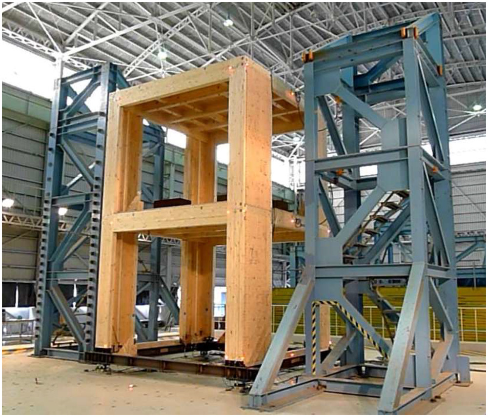
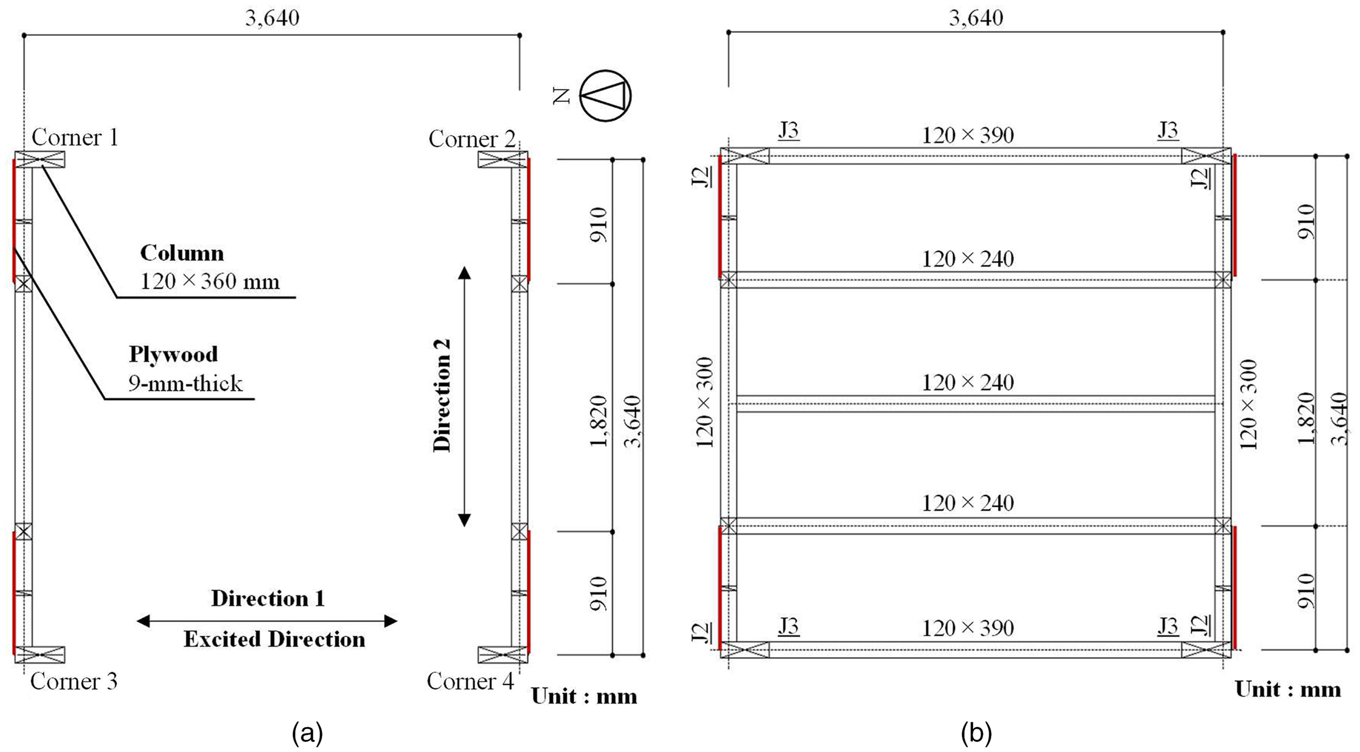
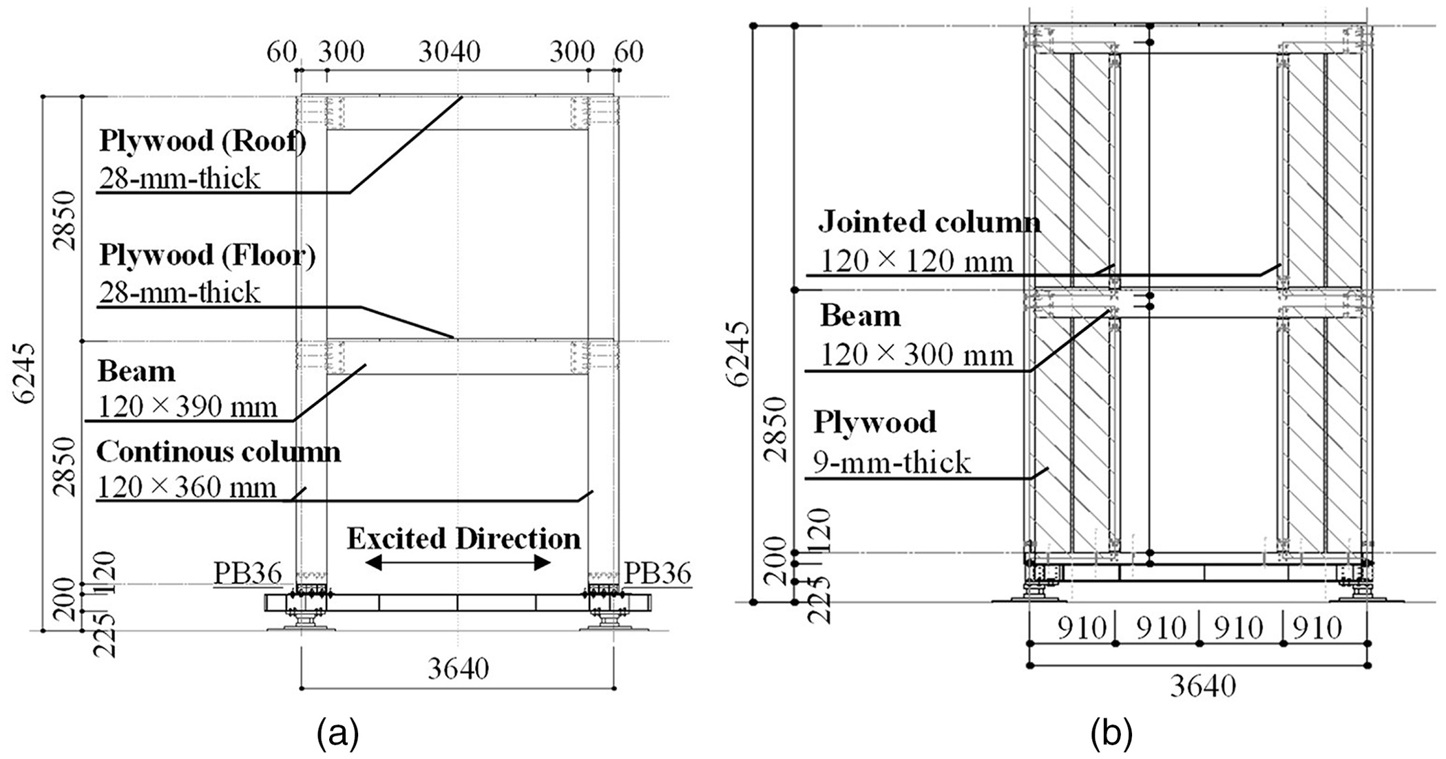
Figs. 1–3 show the photo, plan views, and elevations of the specimen, respectively. The specimen is 3.64 m long in both directions. The test specimen is a 2-story box-type timber construction with the joint’s rotational resistance as the main seismic element in the excited direction (direction 1). Shear walls were installed in the perpendicular (direction 2) to direction 1. The contribution of the shear walls is quite small, and we intended that the seismic performance of this specimen depends on the moment-resistance of joints in direction 1. Fig. 1 shows elevations of MRTF and shear walls. Figs. 2 and 3 also show the section size of each member. The section size of the continuous column in the corner was , and the material is Glued Laminated Timber (Glulam) composed of Scotch pine (Pinus sylvestris, E95-F315), compliant with Japanese Agricultural Standard [JAS, Notification 1152 of the Ministry of Agriculture, Forestry, and Fisheries (2013)]. Accordingly, the mean value of elastic modulus of all layers is greater than . The material of beams is Glulam composed Scotch pine (Pinus sylvestris, E105–F300), and the mean value of elastic modulus of all layers is greater than . JAS has no regulation for the upper limit in these values such as elastic modulus. However, if the timber has more large strength and elastic modulus, the grade will be ranked higher.
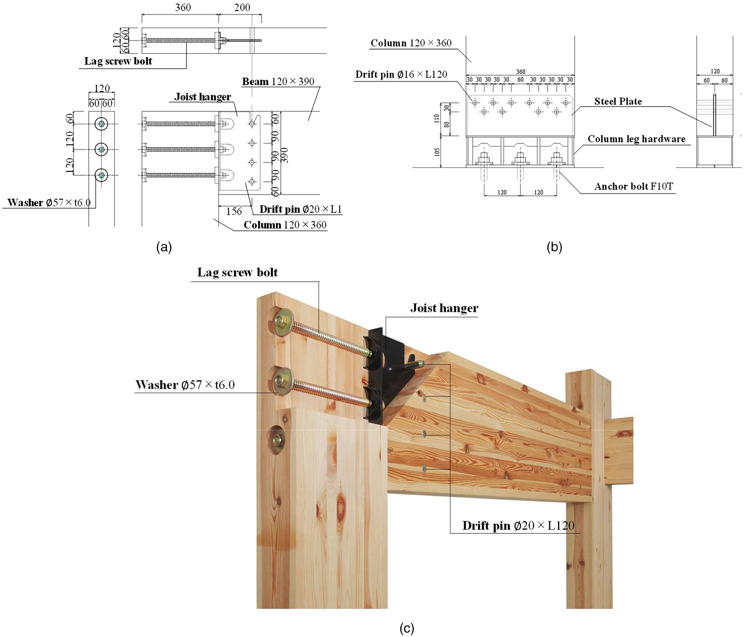
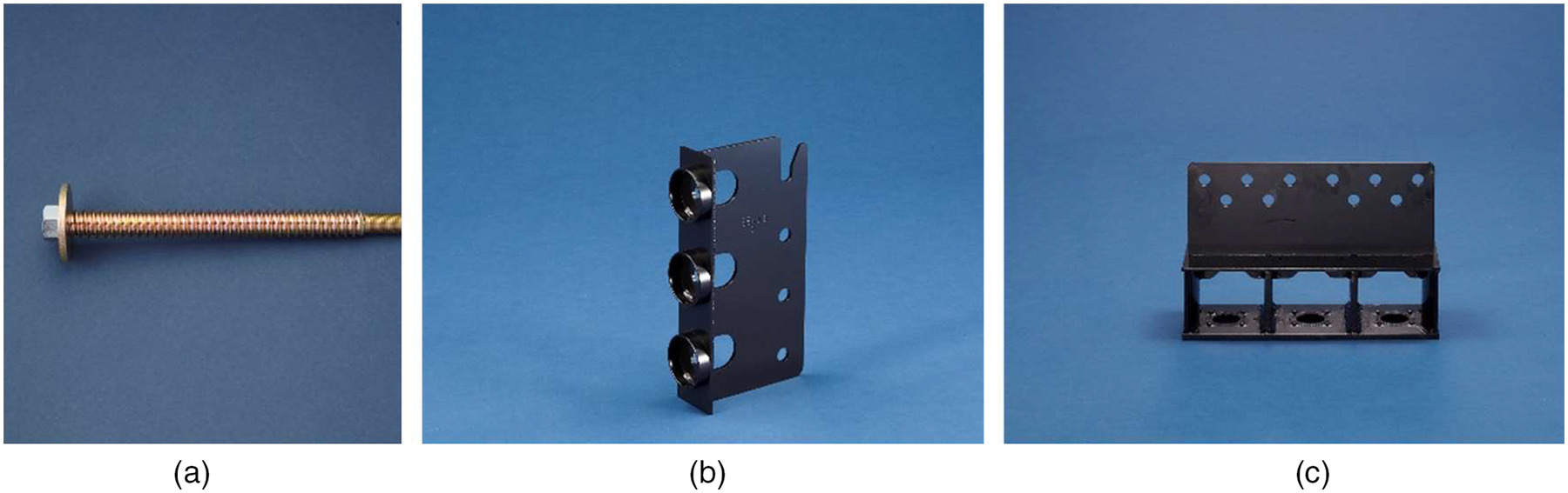
The details of connectors and joints are shown in Figs. 4 and 5, respectively. Beam–column joints had lag screw bolts and a joist hanger, and the column was fixed to the foundation by column leg hardware and anchor bolts. Lag screws, shown in Fig. 5, have benefits of minimal loosing and slippage during the initial application of loads and are increasingly used to join timber members. The tensile stiffness of a lag screw bolt is higher than the normal bolt due to the meshing between the bolt and timber. The joist hanger at the edge of the beam is fixed by the lag screw bolts to the column. This installation method is very easy on-site, which is one of advantages of this connection system. Joist hangers indicated in Fig. 5(b) were used to connect the beam and column and column leg hardware indicated in Fig. 5(c) was used to fix the column to the foundation. Photos in Fig. 6 show details of the joints in the stories and foundation.

The shear walls of 9 mm thick in the first and second layers were nailed with CN50 according to Japanese Industrial Standard (JIS) at nail spacing of 50 and 100 mm, respectively. The floor material was plywood with a thickness of 28 mm and nailed with CN75 according to JIS at a nail spacing of 150 mm. To simulate the mass condition corresponding to a 2-story structure, the design weight of each floor was calculated in consideration of the dead load and live load, and additional seismic masses of 30 kN and 20 kN were placed on the second floor and the roof floor, respectively.
The capacity of the moment-resisting joint (Ma) was defined by the results of the tensile and bending experiments. When the force 1.5 times as strong as the force generated by a moderate earthquake was considered, the ratios of the moment (M) and moment capacity of the joint (Ma) in the specimen was below 0.50 according to the calculation. Table 1 summarizes results of the linear analysis in ASD for the specimen. The shear tests for the walls were also conducted, and these results were used to construct the analysis model. The interstory drift of the first and second stories were 15.39 and 16.33 mm (0.05%), respectively. These results are discussed with experimental results in next section.
| Story | Required shear force (kN) | Interstory drift (mm) | Interstory deformation angle (rad) | OK or NG [ (rad)] | Ratio (result/law) | |
|---|---|---|---|---|---|---|
| 0.2 | 1 | 14.25 | 10.26 | OK | 0.54 | |
| 2 | 7.19 | 10.89 | OK | 0.57 | ||
| 0.3 | 1 | 21.38 | 15.39 | OK | 0.81 | |
| 2 | 10.78 | 16.33 | OK | 0.86 |
Testing Program
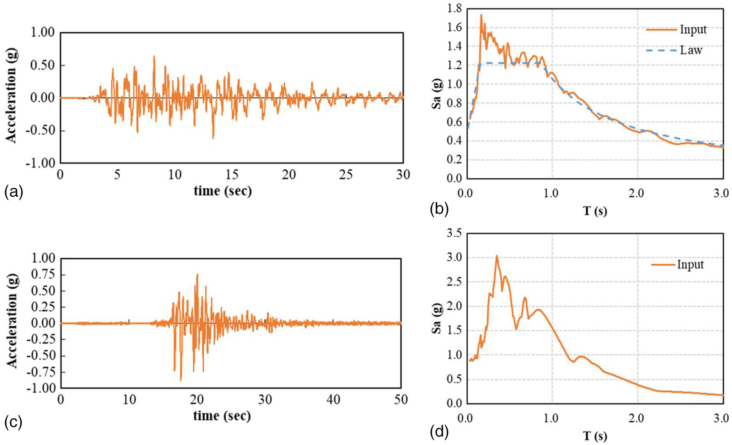
The excitation of the test is produced by a unidirectional full-scale shaking table using three ground motions conducted in the laboratories of the National Institute for Earth Science and Disaster Prevention (NIED) in Tsukuba, Japan. Fig. 7 summarizes the input ground motion. In the tests, two types of waves were utilized for input ground motions. The first was the wave defined in the Japanese BSL, 17% of the wave (BSL17%) is equivalent to a moderate earthquake and 85% of the wave (BSL85%) is equivalent to a severe earthquake for a 2-story building in BSL. The maximum accelerations of the waves for the cases BSL17% and BSL85% are and , respectively. In Japanese law, 100% of the wave shown in Fig. 8 was defined to design the mid- to high-rise building with more than 5 stories. When 100% of the wave was added in a 2-story building, shear force will be higher than those calculated using Eq. (1) in ASD. Reduction factor 17% and 85% are to make it equal to shear force in the ASD and seismic event. The second wave was the Japan Meteorological Agency (JMA) Kobe wave observed in the Osaka-Kobe Earthquake of 1995; this type of wave is often used to represent an extremely severe earthquake beyond the BSL for shaking table tests. The maximum acceleration of the 1995 JMA Kobe wave was . Before and after each shaking test, the specimen was subjected to white noise excitation to obtain natural frequency. We call test 1 “BSL17%,” test 2 “BSL85%,” and test 3 “JMAkobe100%.”

The accelerations and displacements of the specimen during the tests were measured. The accelerations of the floors and shake table were measured by eight accelerometers: two of them on the shake table, three at the second floor, and three on the roof floor.
Experimental Results
Frequency Response
The results from all white noise tests are provided in Table 2, where the natural frequency of the structure ranges from 2.78 to 1.27 Hz. The initial first natural frequency was 2.78 Hz. After BSL17% and BSL85%, the natural frequency decreased 2 and 35%, respectively. The reduction of after BSL17% is 2%, which means this specimen remained undamaged after the moderate earthquake but was slightly damaged after BSL 85%. After JMA Kobe, it decreased 54% and the reduction rate was the largest due the damage of the structure.
| Test | Natural frequency (Hz) | Difference (%) |
|---|---|---|
| Before BSL17% | 2.78 | — |
| After BSL17% (before BSL85%) | 2.72 | |
| After BSL85% (before JMAkobe100%) | 1.82 | |
| After JMAkobe100% | 1.27 |
Load-Deformation Properties
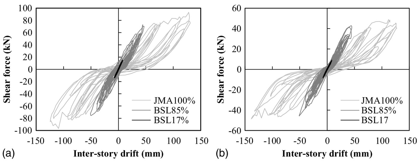
Fig. 8 represents the displacement profile of the specimen for each test, with the profile constructed using the average maximum displacement of the story relative to the shaking table. Fig. 9 shows the relationships of shear force and interstory drift of the first and second stories. Across all tests, primarily a first mode response was observed, with the peak interstory drift for each story occurring simultaneously to the peak displacement. After the first wave BSL17% was input to the specimen in test 1, the maximum interstory of the first and second stories were 7.92 and 8.62 mm, respectively. In other words, the maximum interstory drift was about 1/360 rad and within the damage limit deformation angle for wooden house in a moderate earthquake according to the BSL. In test 2 (BSL 85%), the maximum interstory drift of the first and second stories were 50.81 and 51.08 mm, respectively. In other words, the maximum interstory drift was about and within the safety limit deformation angle for a wooden house in a severe earthquake according to the BSL. From the figure, a clear yield point was not observed, and the behavior was not plasticized. After the third wave JMA Kobe of intensity 100% was inputted to the specimen, the maximum interstory drift of the first and second stories were 130.78 and 138.00 mm in the test, respectively. In other words, the maximum interstory drift was about . In addition, the residual drifts of the entire building were very small in all tests.
Damage Inspection
The specimen was inspected for damage after each test. Because the specimen was designed to achieve the seismic performance for a moderate earthquake in the design, no visible damage was confirmed after test 1. After tests 2 and 3, the damage mainly occurred at the joints (Fig. 10). After test 2, only a minor crack starting from the drift pin occurred at the column leg (PB36), and the beam sunk into the column at the beam–column joints slightly without major damage. After test 3, the crack at the column leg became larger than that in test 2, and embedment of the beam to column progressed as indicated in Fig. 10(c). Figs. 10(d–g) compare the crack of the column legs (PB36) in four corners after test 3. The cracks were different in all corners. In corner 1, the crack was relatively large. On the other hand, there was no crack in corner 2. This phenomenon was considered due to the variations in materials and construction.

Comparison of Linear Analysis in the Design and Experimental Results
Table 3 compares the linear pushover analysis in the design and experimental results. Because the ground motion in test 1 was equivalent to a moderate earthquake, we compared the experimental results in test 1 and the linear analysis for a design shear force when is set as 0.2. As analytical results, the interstory drifts of first and second stories were 10.26 and 10.89 within the damage limit deformation angle , respectively. The ratios of experimental results and the results of analysis were 1.29 and 1.26, respectively, and the experimental values were almost 30% smaller than the those obtained in analysis. This indicates that the design tends to have a large margin to simulate the actual behavior in the seismic event to produce the conservative design of the structure. The analysis in the design should be conservative to ensure the seismic performance. This finding shows that the design method can ensure the seismic performance when is set as 0.2, which is equivalent to a moderate earthquake at least.
| Story | Maximum interstory drift (mm) | Ratio | |
|---|---|---|---|
| Analytical result in ASD | Experimental result | ||
| 1 | 10.26 | 7.92 | 1.29 |
| 2 | 10.89 | 8.62 | 1.26 |
Time History Response Analysis
Analysis Model
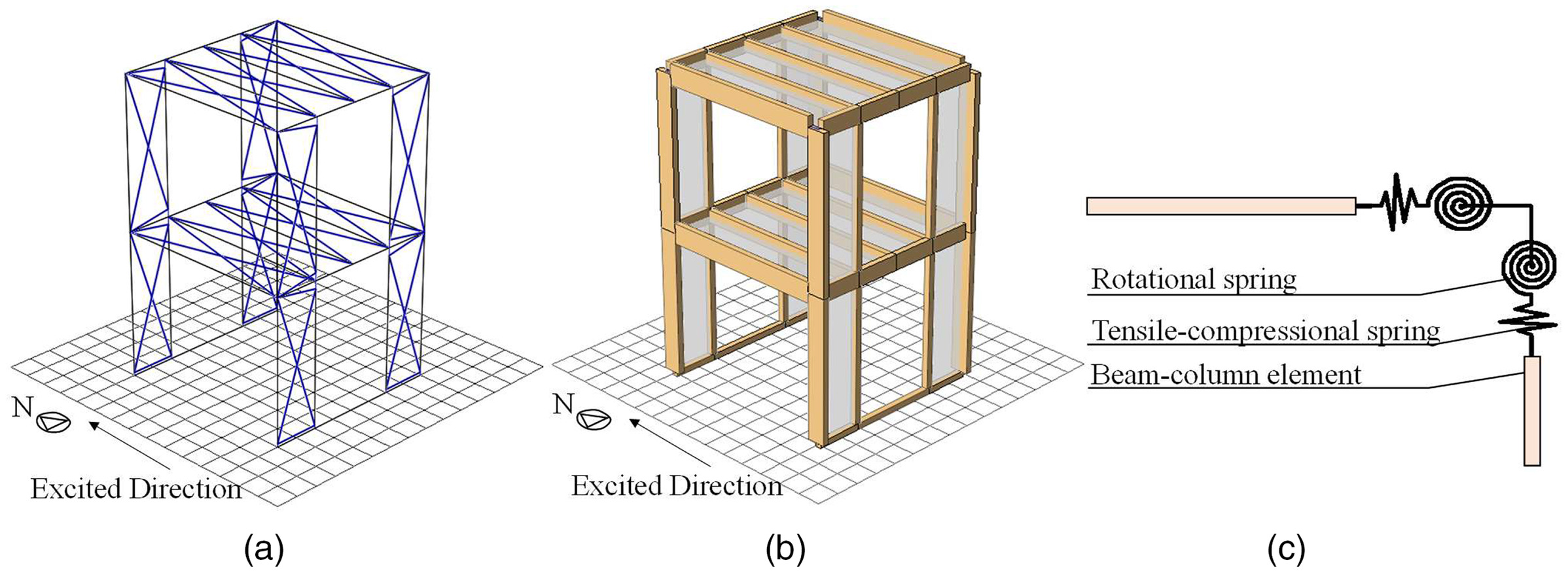
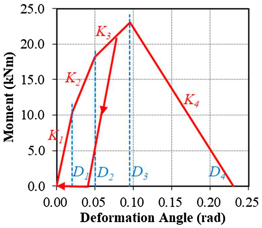
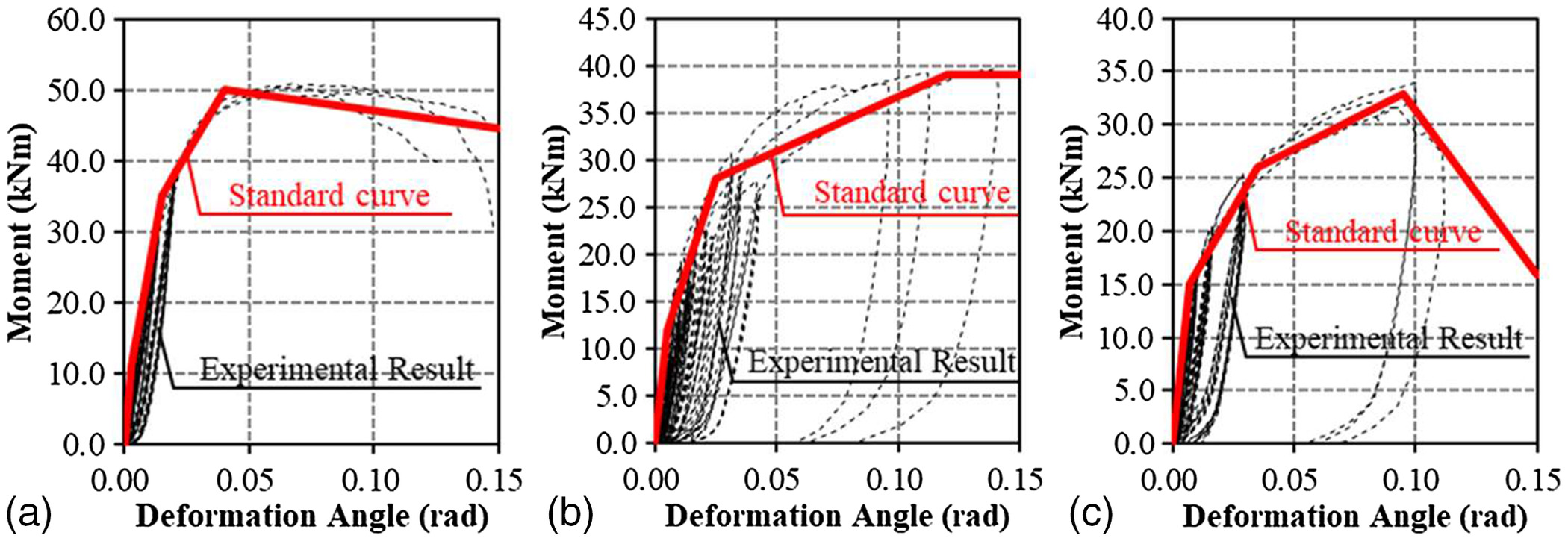
To analyze responses of the wooden structures, we developed and used the wallstat ver.4.3.11. The time-response analysis conducted in the wallstat was based on three-dimensional nonlinear time-history response analysis, as adopted from the extended distinct element method (EDEM) (Meguro and Hakuno 1991). This modeling approach is fundamentally based on a noncontinuum analysis method, the distinct-element method (Cundall 1971), which enables analyzing significant deformation of a fracture-developing process and simulating the three-dimensional seismic response, such as the collapse or rocking motion of a building (e.g., Nakagawa and Ohta 2003a, b; Nakagawa et al. 2013; Sumida et al. 2020). In the wallstat, the analysis model is composed of two primary components: beam–column elements and nonlinear lateral load–resisting shear wall elements. Fig. 11 shows the outline of the analytical model. The beams and columns were modeled as beam–column elements having an elastoplastic rotational spring at the end of the element. According to JAS, Young’s modulus was set to for the column, the other members were set to , and the bending strength was set to in consideration of actual performance. Each joint is modeled as an elastoplastic tensile compressional spring. Hysteretic characteristics of the tensile and compressional springs are set as one side elastic and one side slip types, respectively. In preparation for determining the mechanical properties of tensile, rotational springs, and shear walls, the tensile and bending experiments of the joints and shearing tests for walls were conducted. Each joint’s hysteretic behavior can be characterized using the experimental results and we derived skeleton curves of the moment and the deformation angle relationship for each joint. Fig. 12 shows the outline of the slip backbone curves of the rotational spring. Fig. 13 and Table 4 indicate the rotational hysteretic parameters for each joint (standard backbone curve). Five parameters describe the hysteretic characteristics. Using the shearing test result, brace-replaced springs with tensile compression springs are modeled for each shear wall.
| Name | Stiffness (kNm/rad) | Deformation angle (rad) | |||||
|---|---|---|---|---|---|---|---|
| PB36 (column–foundation) | 3,667 | 2,000 | 600 | 0.003 | 0.015 | 0.040 | |
| F2_2FL (beam–column) | 1,292 | 431 | 62 | 0.005 | 0.025 | 0.120 | |
| F2_RFL (beam–column) | 1,154 | 212 | 63 | 0.007 | 0.035 | 0.095 | |
| J3_2FL (beam–column) | 2,400 | 800 | 116 | 0.005 | 0.025 | 0.120 | |
| J3_RFL (beam–column) | 2,143 | 393 | 117 | 0.007 | 0.035 | 0.095 | |
Measured acceleration at the center of the shaking table was input as ground motions in the numerical analysis. Instantaneous stiffness-proportional damping was used with a coefficient of 2.0% for analytical convenience. When instantaneous stiffness became negative, the damping coefficient was assumed to be zero. All dynamic time-history results were produced using the wallstat program using a time-integration step of . The model weights are set to equal the actual weights of the specimen in the full-scale shaking table test, including the weights of members and the weights of the first and second floors were set to 42.7 and 30.2 kN, respectively.
Time-History Response Analysis
First, we conducted time-history analysis using the standard backbone based on the experimental results of the joints and walls. While the linear analysis in the design is a conservative method, to estimate the deformation in tests, we conducted the analysis based on experiments of the joints. In the design, capacities of the joints are set to be the 95% lower limit of capacity. In the analysis, we set average value as the capacity in the experiments of joints and backbone curves. Fig. 14 shows the results of the analysis of tests 1, 2, and 3. The stiffness was low compared with the experimental result in both the first and second stories in all tests. This problem was also seen in previous studies of MRTF structure [e.g., Nasu et al. (2007)]. To solve the problem, we conducted the data assimilation to get analytical parameters closer to the experimental results and analyze the mechanism.

The Outline of Data Assimilation
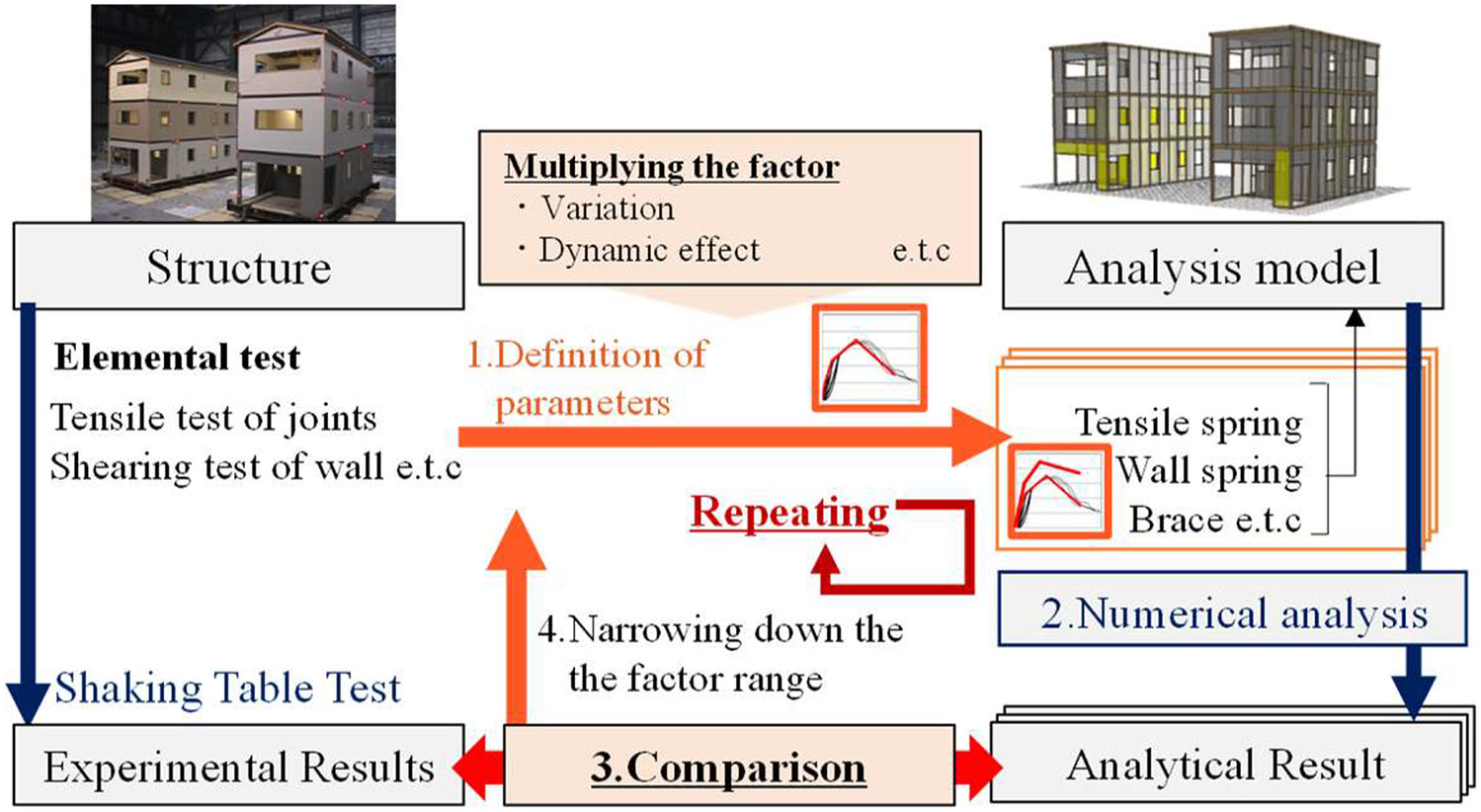
Fig. 15 provides an overview of the data assimilation using orthogonal arrays (OAs) suggested by Kado et al. (2021). We tried the data assimilation for all tests. First, various skeletal curves are created by multiplying the parameters that simulate elemental experiments by correction factors (1. Definition of the Parameters). These parameters are set as the backbone curves of the springs in the analysis model, and multiple analyses are conducted (2. Numerical Analysis). The results of the multiple analyses are compared with the experiments, and the correction factor range are analyzed (3. Comparison). Then, the factor ranges are narrowed down by reviewing the range (4. Narrowing Down the Factor Range). Data assimilation was attempted by repeating these cycles multiple times. In this study, we were able to obtain accurate results by repeating this process four times. The details of the flow are described as follows:
Definition of the Parameters
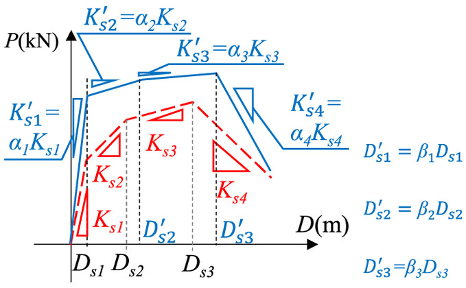
In the shaking table test, the moment stiffness of the joint has the greatest effect on the behavior. The results of Frenette et al. (1996) and Heiduschke et al. (2009) revealed that in general, most of the drift of the timber frames (85%–95%) arose from the joint rotations, while only a small part (10%–15%) was due to the bending of the columns. These results suggest the stiffness of the joints is the key factor for the drift in the MRTF. Therefore, mainly focusing on the rotational spring input parameters for the joints, correction factors were multiplied to set the skeleton curve of the rotational spring. In addition, Young’s modulus was also focused. The correction factor multiplied to the parameters are indicated in Fig. 16. In the shaking table test, interstory drift reached 0.04 rad and all joints did not experience the maximum capacity of each joint. Therefore, we changed the analytical parameters within 0–0.04 rad. The characteristic values were the 1st to 3rd stiffness ( to ) and the 1st to 2nd points ( to ). For the backbone curves, , where is defined as the initial stiffness of the skeletal curve tracing the element experiment multiplied by a correction factor from 0.5 to 2.0, and and are defined as the ratio of the stiffness to the previous stiffness, respectively, greater than 0 and less than 1, multiplied by their previous stiffness. There are three types of rotational springs (PB36, F2, and J3) used in this specimen, and the correction factors were multiplied to the rotational springs in the first and second layers, respectively.
Taguchi (1994) methods are statistical and based on the design of experiments (DOE), also called quality engineering, to improve the quality of manufactured goods. In the theory, the OA is a factorial-based approach combining statistical and engineering techniques (Mitra 1998). The Taguchi technique uses OAs to analyze numerous variables with fewer experiments (Pignatiello 1988). Moreover, inferences from the reduced number of experiments apply to the entire experimental region spanned by control factors and levels (Phadke 1989). Therefore, this method allows data assimilation of many parameters without too much numerical analysis. Therefore, OAs in the Taguchi method were applied to conduct the time-history response analysis. The OA is a type of general fractional factorial design. It is a highly fractional orthogonal design based on a design matrix proposed by Taguchi and allows one to consider a selected subset of combinations of multiple factors at multiple levels. OAs are balanced to ensure that all levels of all factors are considered equally. Therefore, the factors can be evaluated independently, despite the fractionality of the design. In this study, 12 eleven-level factors and the OA, which is to examine the effects of those factors and called L121, were adopted. In L121, to clarify all effects of 12 eleven-level factors, 121 combinations are planned. Table 5 shows two OAs (L121) that target the 11 significant analytical parameters of rotational springs and Young’s modulus, along with the factor levels of the coefficient. The correction factors were set as 11 levels, equally spaced from minimum to maximum. In the numerical analysis, we multiplied the coefficient and the property. If we try to conduct all combinations, () cases are simulated. Using combination of two OAs, 14,641 () cases are needed.
| Group | No. | Name of the factor | Factor levels (coefficient) 1–11 | |
|---|---|---|---|---|
| 1 | 1 | PB3 | K1 | 0.5–2.0 |
| 2 | K2 | 0.5–1.0 | ||
| 3 | K3 | 0.8–1.0 | ||
| 4 | D1 | 0.5–2.0 | ||
| 5 | D2 | 0.5–2.0 | ||
| 6 | J3_2FL | K1 | 0.5–2.0 | |
| 7 | K2 | 0.5–1.0 | ||
| 8 | K3 | 0.5–1.0 | ||
| 9 | D1 | 0.6–2.0 | ||
| 10 | D2 | 0.5–2.0 | ||
| 11 | Beam | E | 0.8–2.0 | |
| 12 | Column | E | 0.8–2.0 | |
| 2 | 1 | F2_2FL | K1 | 0.5–2.0 |
| 2 | K2 | 0.5–1.0 | ||
| 3 | K3 | 0.8–1.0 | ||
| 4 | D1 | 0.5–2.0 | ||
| 5 | F2_RFL | K1 | 0.5–2.0 | |
| 6 | K2 | 0.5–1.0 | ||
| 7 | K3 | 0.5–1.0 | ||
| 8 | D1 | 0.5–2.0 | ||
| 9 | J3_RFL | K1 | 0.6–2.0 | |
| 10 | K2 | 0.5–1.0 | ||
| 11 | K3 | 0.5–1.0 | ||
| 12 | D1 | 0.5–2.0 | ||
Numerical Analysis
The analyses planed in phase 1 were conducted using JAXA’s HPC . Using a common computer will take 300 days but using the supercomputer , it took 5 hours to complete 14,641 analysis cases.
Comparison
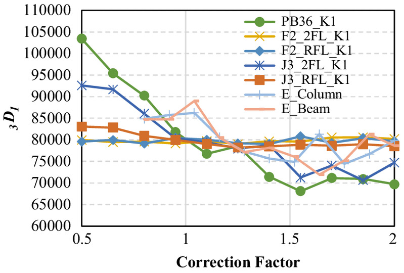
Focusing on the interstory drift measured in the full-scale shake table tests, the difference between the analytical and experimental results were estimated for each story. The factorial effect diagram of quality engineering was used to evaluate the analytical results. The diagram is used to identify input parameters that are sensitive to output parameters and to analyze the range of correction factors that reduce the difference between experimental and analytical results.
The distances between the plots of interstory drift in the analysis and those in the experiment were summed for every 0.01 sampling period according to Eq. (2)where is the interstory drift of story in the time-response analysis (mm); is the interstory drift of story in the test (mm); is the test number ( BSL17%, BSL85%, JMAkobe100%); is the story number; and is the time (s).
(2)
The results are analyzed in this phase to determine whether the analysis result was close to the experimental results or not. First, conducting 14,641 analysis cases, the relationship between these values and the factor of the joint characteristics was confirmed. Fig. 17 shows the effect of the analytical parameters of each rotational spring. The horizontal axis indicates the factor, and the vertical axis shows the estimation value. Some cases have the same factor of each property, so the value in the figure means the mean value. If a line has a high slope, it shows that the parameter significantly affects the analytical results in the variable range. From Fig. 18, especially for PB36_K1, J3_2FL_K1, E_Column, and E_Beam, the lines have a high slope and the elements are expected to have relatively high impact to the numerical analysis.
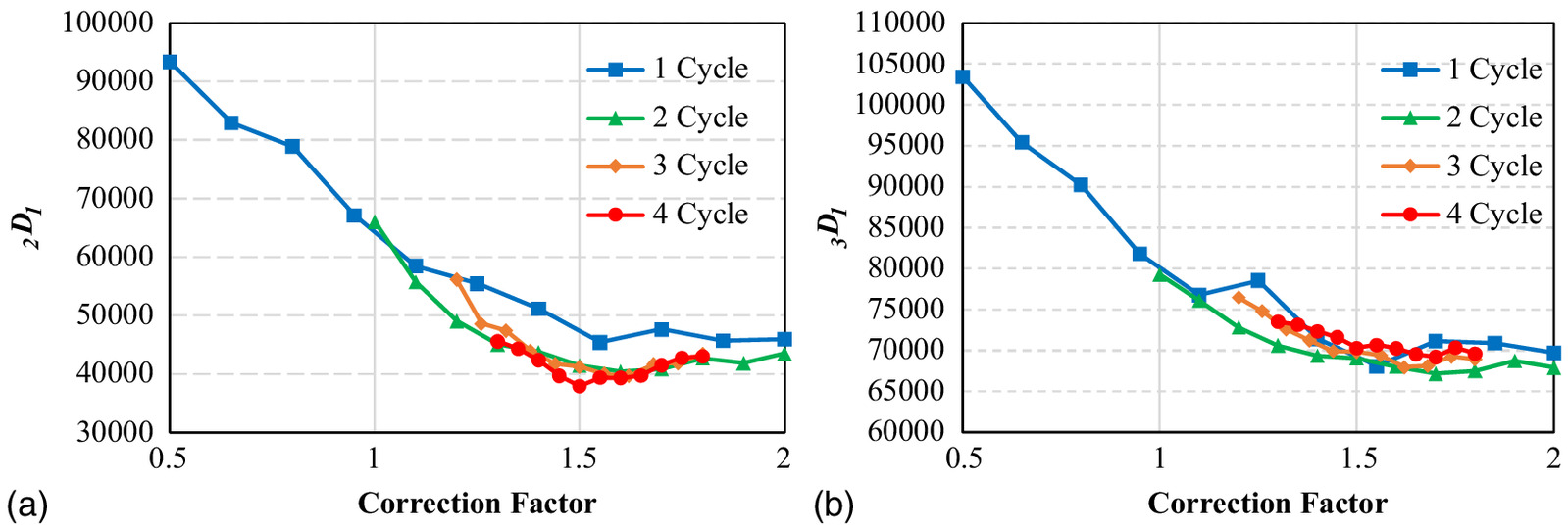
Narrowing Down the Factor Range
To minimize the difference between the analytical and experimental results, the next step is narrowing the factor range of each parameter. From the results in phase 3, we can narrow down the factor range to between 1.0 and 2.0 to obtain a numerical analysis closer to the experimental result. Similarly, we can narrow the ranges of other parameters to move to the second cycle. Next, the same procedure was conducted, and the ranges were narrowed down. For example, from Fig. 18 for PB36_K1, the value is small in the factor range between 1.0 and 2.0. Then we can narrow down the range between 1.0 and 2.0. The factor range of other parameters were narrowed down in similar way. Fig. 18 also shows the graphs of factorial effects after each cycle. After four cycles, for all parameters, the curve changed, and the values decreased when compared with after first and second cycles. As aforementioned, the value in graphs of factorial effect means the mean value of cases with the same factor, so other properties affect the value and the curve. We can say that the interaction effects of analytical parameters with each other decreased and the difference between the analytical and experimental results became small by narrowing the parameter ranges.
Results of Data Assimilation
Figs. 19 and 20 are comparisons of the analytical and experimental results of all tests. We extracted the closest combination of the analytical parameters from 14,641 analysis cases based on the values calculated by Eq. (2) for JMAkobe100%. The stiffness became closer after the data assimilation, the analytical results have a more accurate prediction of the experimental results, and the curve fits better. However, some points have to be revised to get more accurate prediction. For example, for JMAkobe100%, after about 23 s, the deformation is larger than the experimental result. Isoda et al. (2021) compared some hysteretic rules and clarified that there is much difference after the structure experienced maximum deformation to reproduce the experimental behavior. This indicated that a more accurate simulation is expected to occur by development of the hysteretic rule after 23 s in JMAkobe100% and revision of the damping. On the other hand, in BSL17%, the stiffness in the analysis is higher than those in the test. These analytical results occurred to reproduce the behavior at large deformation, so the accuracy of analysis at small deformation should be revised to simulate accurately. Fig. 21 shows the time-history curves of the deformation angle of joints in the north corner. The deformation angle is matched well with the experiment before 23 s. As aforementioned, this also depends on the hysteretic rule.
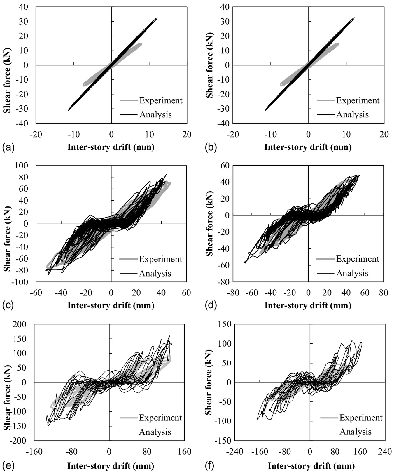
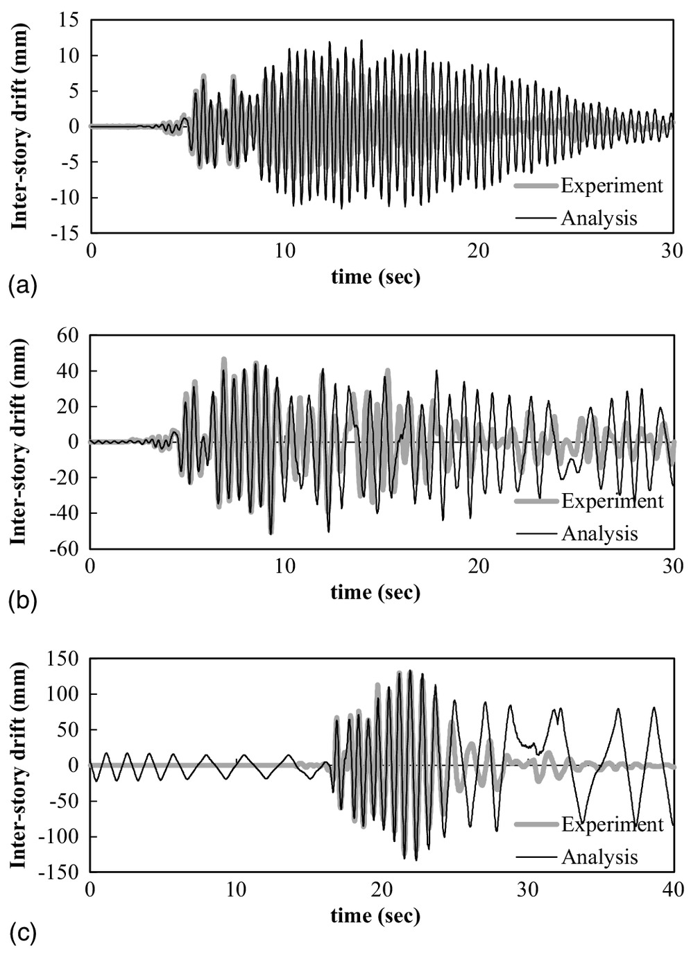
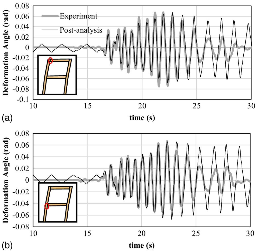
Fig. 22 shows analytical parameters ranked in the top five from 14,641 cases in the ascending order of , which targets the interstory drift of the first story in JMAkobe100%. For J2_2FL and PB36, both stiffness and capacity are higher than those in the standard backbone curve. The stiffness of some obtained data was 1.0–1.5 times higher than the properties of the standard skeletal curves obtained from the bending tests. The causes may include dynamic effect or influence of the floor. In the analysis model, the floor was modeled to brace-replaced springs, and the out-plane resistance of the floor was ignored. Furthermore, although the floor and placed weights might hold down the rotational behavior of the joint, it was ignored. Although other factors might not have been considered in the analysis model, we confirmed that the analysis results approach the experimental results by increasing the properties of the rotational spring in the analysis model. Therefore, the result indicates that the moment resistance of the floor and joint was higher than expected in analysis before data assimilation. Sakata et al. (2003) studied the stressed-skin effect on the moment-resisting joint and proved that the effect heightened the stiffness and capacity. We can say that one of the causes is stressed-skin effect of the floor. This phenomenon will be useful to estimate the seismic performance of MRTF, and future studies on the structure should include a follow-up study to verify the phenomenon.

As for the Young’s modulus of the member, the top five parameters were all 2.0, as large as those before data assimilation, indicating that the correction factor tended to be larger than that before data assimilation. The timber is manufactured according to JAS standards, which guarantees a minimum Young’s modulus value. However, we can say that the actual performance is considered to be much higher than the law value. Comparison of the actual performance and the law value is also an issue for future study.
The data assimilation allowed us to inductively infer what problems existed in the analysis. These causes, which may not have been taken into account in the analytical model, will be verified in the future through comparison of the behavior of each part and static joint and member tests, and will lead to the prediction of the response of the specimen without experimental results.
In this study, the wave defined in the Japanese BSL and the JMA Kobe wave observed in the Osaka-Kobe Earthquake of 1995 that destroyed many wooden houses were utilized for input ground motions and clarified the performance as a first step. Japan is located in the subduction zone, but waves that were observed in the Hokkaido and Tohoku earthquakes were not used, and various waves also should be considered to the structure in future studies to clarify the behavior in analysis and experiment.
Conclusions
In this study, full-scale shake table tests were conducted to confirm the seismic behavior of MRTFs designed for allowable stress. Because the allowable stress design was expected to result in large deformation of the MRTF, it was decided to confirm the performance required in the Earthquake Resistance Grade 3. This design method is to secure the performance to withstand the force generated by 1.5 times moderate earthquake without damage. The structure experienced a maximum deformation angle of against the damage-limiting criterion of for the moderate earthquake, and no visible damage was observed. The next large earthquake required a criteria as the safety limit, and the maximum interstory angle was only about . It was confirmed that there was no significant damage, and the deformation was limited to the same level as that of a shear wall structure. Next, the specimens did not collapse even after JMAkobe100%. The specimen was designed within the elastic range for moderate earthquakes, but it did not collapse against a PGA of .
Elemental tests of joints defined the parameters of the structural analysis model, and a time-history analysis was conducted. It is not possible to trace the full-scale experiment properly. Therefore, data assimilation was performed to redefine the parameters that could be reasonable. The stiffness of some redefined data was 1–1.5 times higher than the properties of the standard skeletal curves obtained from the bending tests, which may be due to dynamic effects and floor stress-skin effects. This phenomenon should be verified to estimate the seismic performance of the MRTF structure.
Data Availability Statement
Some or all data, models, or code that support the findings of this study are available from the corresponding author upon reasonable request.
Acknowledgments
This research was conducted as part of a collaborative research by Kyoto University, Osaka Institute of Technology, and JAXA, “Examination of data assimilation method for simulation of collapse analysis of wooden houses using quality engineering.” In the time-history response analysis, we used the Japan Aerospace Exploration Agency supercomputer system JSS3. In addition, NCN Co., Ltd. cooperated with the test specimen of the shaking table test.
References
AIJ (Architectural Institute of Japan). 2017. 2016 Kumamoto earthquake damage investigation Report. Tokyo: Architectural Institute of Japan.
Bouchaïr, A., P. Racher, and J. F. Bocquet. 2007. “Analysis of dowelled timber to timber moment-resisting joints.” Mater. Struct. 40 (10): 1127–1141. https://doi.org/10.1617/s11527-006-9210-0.
Cundall, P. A. 1971. “A computer model for simulating progressive, large-scale, movements, in blocky rock system.” In Proc., Int. Symp. on Rock Mechanics, 129–136. Salzburg, Austria: International Society for Rock Mechanics.
Frenette, C., R. O. Foschi, and H. G. Prion. 1996. “Dynamic behavior of timber frame with dowel type connections.” In Vol. 4 of Proc., Int. Wood Engineering Conf., 89–96. Madison, WI: Omnipress.
Guo, J., and Z. Shu. 2019. “Theoretical evaluation of moment resistance for bolted timber connections.” In Vol. 303 of Proc., MATEC Web of Conf. Lisbon, Portugese: NOVA Univ. of Lisbon.
Heiduschke, A., B. Kasal, and P. Haller. 2009. “Shake table test of small- and full-scale laminated timber frames with moment connections.” Bull. Earthquake Eng. 7 (1): 323–339. https://doi.org/10.1007/s10518-008-9075-4.
Hiyama, S., T. Ohira, Y. Yamazaki, H. Sakata, R. Odani, A. Fujishiro, and H. Itoh. 2014. “Study on failure mode and strength estimation of moment resisting timber joint. Part1 Experiment on joint.” In Proc., Summaries of Technical Papers of Annual Meeting, 143–144. Tokyo: Architectural Press Institute of Japan.
Housner, G. W., L. A. Bergman, T. K. Caughey, A. G. Chassiakos, R. O. Claus, S. F. Masri, R. E. Skelton, T. T. Soong, B. F. Spencer, and J. T. P. Yao. 1997. “Special issue; Structural control: Past, present, and future.” J. Eng. Mech. ASCE 123 (9): 897–971. https://doi.org/10.1061/(ASCE)0733-9399(1997)123:9(897).
Isoda, H., M. Matsuda, S. Tesfamariam, and S. Tamori. 2021. “Shake table test of full-size wooden houses versus wall test result: Comparison of load-deformation relationship.” J. Struct. Eng. 35 (5): 04021043. https://doi.org/10.1061/(ASCE)CF.1943-5509.0001609.
Kado, Y., C. Uematsu, A. Takino, T. Namba, and T. Nakagawa. 2021. “Study of data assimilation method using quality engineering and application to the seismic response analysis of wooden houses.” [In Japanese.] In Vol. 26 of Proc., Japan Conf. on Computational Engineering. Tokyo: Japan Society for Computational Engineering and Science.
Kalnay, E. 2003. Atmospheric modeling, data assimilation and predictability. Cambridge, MA: Cambridge University Press.
Kasal, B., P. Guindos, T. Polocoser, A. Heiduschke, S. Urushadze, and S. Pospisil. 2014. “Heavy laminated timber frames with rigid three-dimensional beam-to-column connections.” J. Perform. Constr. Facil. 28 (6): A4014014. https://doi.org/10.1061/(ASCE)CF.1943-5509.0000594.
Komatsu, K. 2016. Glued laminated timber—Architectural history of development. Kyoto, Japan: Kyoto University Academic Press.
Meguro, K., and M. Hakuno. 1991. “Simulation of structural collapse due to earthquakes using extended distinct element method.” In Proc., Summaries of Technical Papers of Annual Meeting, 763–764. Tokyo: Architectural Press Institute of Japan.
Ministry of Agriculture, Forestry, and Fishery. 2013. Japan agricultural standard. Tokyo: Japan Agricultural Standard Association.
Ministry of Construction. 2007. Japan agricultural standard. Tokyo: Japan Agricultural Standard Association.
Mitra, A. 1998. Fundamentals of quality control and improvement. Delhi, India: Pearson Educational Asia.
MLIT (Ministry of Land, Infrastructure, Infrastructure and Tourism). 2008. Allowable stress design method of conventional buildings. Tokyo: Japan Housing and Wood Technology Center.
Nakagawa, M., H. Isoda, and A. Okano. 2009. “Seismic performance evaluation and full-scale shaking table test of timber frame, conventional construction and composite structure.” J. Struct. Constr. Eng. AIJ 74 (636): 321–330. https://doi.org/10.3130/aijs.74.321.
Nakagawa, T., T. Hidaka, and M. Inayama. 2013. “Damage investigation and collapsing process analysis of Myokenji Hondo damaged from the Great East Japan EARTHQUAKE: Part 2 Collapsing process analysis using 3D space frame model.” J. Struct. Eng. B AIJ 59B: 573–578.
Nakagawa, T., and M. Ohta. 2003a. “Collapsing process simulations of timber structures under dynamic loading I: Simulations of two-story frame models.” J. Wood Sci. 49 (5): 392–397. https://doi.org/10.1007/s10086-002-0500-z.
Nakagawa, T., and M. Ohta. 2003b. “Collapsing process simulations of timber structures under dynamic loading II: Simplification and qualification of the calculating method.” J. Wood Sci. 49 (6): 499–504. https://doi.org/10.1007/s10086-002-0507-5.
Nasu, H., H. Ishiyama, N. Yamamoto, M. Takaoka, T. Miyake, and H. Noguchi. 2007. “Shaking table test of full scale 3-story timber frame.” J. Struct. Constr. Eng. AIJ 72: 129–135. https://doi.org/10.3130/aijs.72.129_2.
Noda, T., H. Isoda, T. Mori, K. Moritani, M. Shinohara, R. Hosomi, S. Kurumada, and T. Makita. 2019. “Development of original construction method with combination of CLT core wall and wood frame member (No. 5 analytical consideration of 3-story full scale shaking table test).” In Proc., Summaries of Technical Papers of Annual Meeting, 697–698. Tokyo: Architectural Press Institute of Japan.
Ohira, R., Y. Yamazaki, H. Sakata, R. Odani, A. Fujishiro, and H. Itoh. 2014. “Study on failure mode and strength estimation of moment resisting timber joint part 2 failure mode and strength estimation.” In Proc., Summaries of Technical Papers of Annual Meeting, 145–146. Tokyo: Architectural Press Institute of Japan.
Phadke, M. S. 1989. Quality engineering using robust design. Englewood Cliffs, NJ: Prentice-Hall.
Pignatiello, J. J., Jr. 1988. “An overview of the strategy and tactics of Taguchi.” IIE Trans. 20 (3): 247–254. https://doi.org/10.1080/07408178808966177.
Sakata, H., Y. Matsubara, and A. Wada. 2003. “Experimental study on moment resisting timber joint using stressed-skin effect.” J. Struct. Constr. Eng. AIJ 68 (Aug): 143–150. https://doi.org/10.3130/aijs.68.143_2.
Solario, F., L. Giresini, W.-S. Chang, and H. Huang. 2017. “Experimental tests on a dowel-type timber connection and validation of numerical models.” Buildings 7 (4): 116. https://doi.org/10.3390/buildings7040116.
Sumida, K., H. Isoda, T. Mori, R. Inoue, K. Tanaka, and T. Sato. 2019. “Survey of construction situation in Mashiki town two years after the 2016 Kumamoto earthquakes.” J. Jpn. Assoc. Earthquake Eng. 19 (1): 21–33. https://doi.org/10.5610/jaee.19.1_21.
Sumida, K., T. Nakagawa, and H. Isoda. 2020. “Seismic testing and analysis of rocking motions of Japanese post-and-beam construction.” J. Struct. Eng. 147 (2): 04020323. https://doi.org/10.1061/(ASCE)ST.1943-541X.0002901.
Taguchi, G. 1994. Quality engineering for technology development. Tokyo: Japanese Standards Association Group.
Information & Authors
Information
Published In

Journal of Structural Engineering
Volume 149 • Issue 7 • July 2023
Copyright
This work is made available under the terms of the Creative Commons Attribution 4.0 International license, https://creativecommons.org/licenses/by/4.0/.
History
Received: Oct 17, 2022
Accepted: Jan 18, 2023
Published online: Apr 25, 2023
Published in print: Jul 1, 2023
Discussion open until: Sep 25, 2023
ASCE Technical Topics:
- Allowable stress design
- Building design
- Building materials
- Design (by type)
- Earthquake engineering
- Engineering fundamentals
- Engineering materials (by type)
- Engineering mechanics
- Frames
- Geotechnical engineering
- Joints
- Materials engineering
- Moment (mechanics)
- Seismic design
- Seismic tests
- Statics (mechanics)
- Structural design
- Structural engineering
- Structural members
- Structural systems
- Tests (by type)
- Wood and wood products
Authors
Metrics & Citations
Metrics
Citations
Download citation
If you have the appropriate software installed, you can download article citation data to the citation manager of your choice. Simply select your manager software from the list below and click Download.