Investigating Sewer Parameters Leading to Manhole Corrosion: A Case Study from the City of Arlington, Texas
Publication: Journal of Environmental Engineering
Volume 150, Issue 5
Abstract
A sewer system is a principal element of infrastructure in modern cities, accounting for massive amounts of public investments. Corrosion of manholes in the sewer system is a global issue, and millions of dollars are being spent on the maintenance, restoration, and replacement of deteriorated sewer networks. Concrete manholes in the sewer system are deteriorating due to the attack of sulfuric acid produced by microorganisms in a process termed microbial induced concrete corrosion (MICC), which reduces the lifespan of concrete sewer elements. The objective of this paper is to investigate the correlation between the gas- and liquid-phase sewer environmental factors and hydrogen sulfide concentration in the gas phase. The production, emission, and build-up of hydrogen sulfide gas in manholes is identified as a major cause of MICC in manhole shafts. The field study was conducted in more than 200 manholes in the City of Arlington (Texas, US). The data was collected every minute for 48 h to understand the trends of liquid- and gas-phase parameters such as hydrogen sulfide ( concentration), liquid and gas temperature, pH, DO, and relative humidity. The study also examines how gas-phase concentrations vary with season; manhole design, including manholes’ depth, slope, and presence of drop; and sewer flow conditions such as velocity and turbulence. Although no strong linear correlation was found between liquid-/gas-phase parameters, the manhole categories were found to play a significant role in generation. The manholes with hydraulic jump generated the highest average concentrations, followed by manholes with drops. High turbulence zones were observed in manholes of both categories, leading to stripping from liquid to gas phase. The highest concentration was recorded in summer, suggesting that higher liquid temperature resulted in increased bacterial activity, which generated greater liquid-phase sulfide. Greater Henry’s law constants in summer, due to high temperatures, would have favored transfer of liquid-phase sulfide to the gas phase.
Introduction
A sewer system is a principal element of infrastructure in modern cities, accounting for massive public investments made over decades. Corrosion of manholes in the sewer system is a global issue with substantial economic relevance, environmental health, and safety issues, specifically in regions having warmer climates. There are around 550,000 km of concrete pipes in the US (Romanova et al. 2014), and the total asset value of the sewer networks is estimated to be about $1 trillion. Millions of dollars are being spent globally on maintenance, restoration, and replacement of deteriorated sewer networks. In the US alone, sewer asset loss around $14 billion per annum is expected due to the corrosion of sewer pipes (Koch et al. 2002).
The production, volatilization, and build-up of hydrogen sulfide gas in manholes is identified as a major cause of structural degradation. The deterioration occurs due to microbial induced concrete corrosion (MICC), where the concrete is corroded due to the sulfuric acid formed by the oxidation of hydrogen sulfide gas that volatilizes into the headspace of manholes. This can lead to infrastructure failures such as manhole lids dropping through the structure, sewers overflowing, and cracking of the sewer pipes and in adverse cases could result in street collapses, creating a safety hazard (Jiang et al. 2015; O’Connell et al. 2010; USEPA 1991).The expected design life of the concrete manhole can be reduced from 100 years to 30–50 years and, in extreme cases, even to 10 years (Jensen et al. 2009).
The physiochemical and biological processes leading to sewer pipe corrosion have been studied since 1940, and Parker was first to report the theory behind the MICC process (Parker 1945, 1947, 1951). The colonization of acid-producing autotrophic microbes on the concrete reduces sulfate to sulfide and further to hydrogen sulfide (USEPA 1992). Depending on pH of the wastewater, hydrogen sulfide dissociates to dissolved hydrogen sulfide gas (), hydrosulfide ion (), and sulfide ion () (Hao et al. 1996). The gas combines with the moisture on the nonsubmerged surfaces of pipe and is biologically oxidized to sulfuric acid (), which dissolves the cement (calcium carbonate binder), leading to concrete corrosion (Roberts et al. 2002; Wei et al. 2010). Literature manifests the theory behind the MICC process; rigorous research and development studies on MICC began in the 1980s, when corrosion rates were significantly rising, due to improved living conditions posing threats to decades old sewer systems. Surges in protein consumption, along with use of hot water and sulfur-containing detergents in households, have contributed to increased risk of corrosion (Romanova et al. 2014).
Much research has been conducted on MICC and is broadly classified into two categories. The first category includes studies based on the corrosion mechanism and factors that control the rate of MICC, while the second category includes research on innovative techniques and strategies for corrosion resistance. The former primarily consists of laboratory studies examining several individual facets of corrosion mechanisms related to MICC (Wells and Melchers 2014, 2015), and conclusions drawn based on experiments conducted in controlled environments (Li et al. 2019). Corrosion rates from accelerated or aggressive laboratory setups or simulation chambers often overestimate rates, as it is nearly impossible to replicate the natural field environmental conditions leading to MICC. These studies compare MICC on different concrete mixes or protective coatings but do not provide insights on the relevance of individual factors affecting MICC in the natural environment. Lack of reliable field data and thorough understanding of the interaction between key parameters were key concerns. An in situ study conducted by Romanova et al. (2014) explored the relation between various parameters; however, conclusions were made from studying only two manholes for a period of two months, which is comparatively a short period of time and data.
The second category of studies aimed to achieve longer service life for the MICC prone structures. These include chemical dosing of wastewater (Ganigue et al. 2011; Jiang et al. 2011, 2013; Jiang and Yuan 2013), concrete treatment methods including application of biocides (Li et al. 2020; Sun et al. 2015), antimicrobial coatings (Berndt 2011; Haile and Nakhla 2010; Kaushal et al. 2018; Lebrero et al. 2011; de Muynck et al. 2009) and inhibitors (Saraswathy and Song 2007), collection and treatment of hydrogen sulfide enriched sewer gas from sewer (Jiang et al. 2017; Parande et al. 2006; Wang et al. 2010), and the development of bio-concrete (Song et al. 2021; Zhu and Dittrich 2016). To date, there is a severe gap in studies that investigated the factors leading to manhole shaft MICC in actual sewer environments. Also, the previous studies were inadequate in providing insights about how a manhole’s design and flow conditions inside the sewer system affect the concentration in manholes.
This study aims to investigate gas- and liquid-phase sewer environmental factors leading to microbially induced concrete corrosion in manhole shafts and the correlation between these factors to better understand MICC in manhole shafts. The hourly trend of liquid- and gas-phase parameters such as concentrations, liquid and gas temperature, pH, DO, and relative humidity were evaluated. In addition, the study also examines the effect of seasonal variations; the impact of manhole designs, including manholes’ depth, slope, and presence of drop; and sewer flow conditions such as velocity and turbulence.
Methods
The study was conducted in the City of Arlington (Texas, US). Over the course of the year, the temperature typically varies from 37°F to 96°F and is rarely below 25°F or above 102°F. The data collection spanned from August 2017 to February 2019. More than 200 manholes with varying manhole configurations were studied (Table 1).
| Manhole category | Number of manholes |
|---|---|
| Drop | 18 |
| Drop between 2′ and 0.2′ | 27 |
| Standard drop 0.1′ | 68 |
| Pipe diameter: uniform | 64 |
| Pipe diameter: smaller to larger | 36 |
| Pipe diameter: larger to smaller | 11 |
| Supercritical flow | 68 |
| Subcritical flow | 36 |
| Hydraulic jump | 25 |
| Bends | 88 |
| Multiple inlets | 50 |
Note: A manhole might fall into multiple categories.
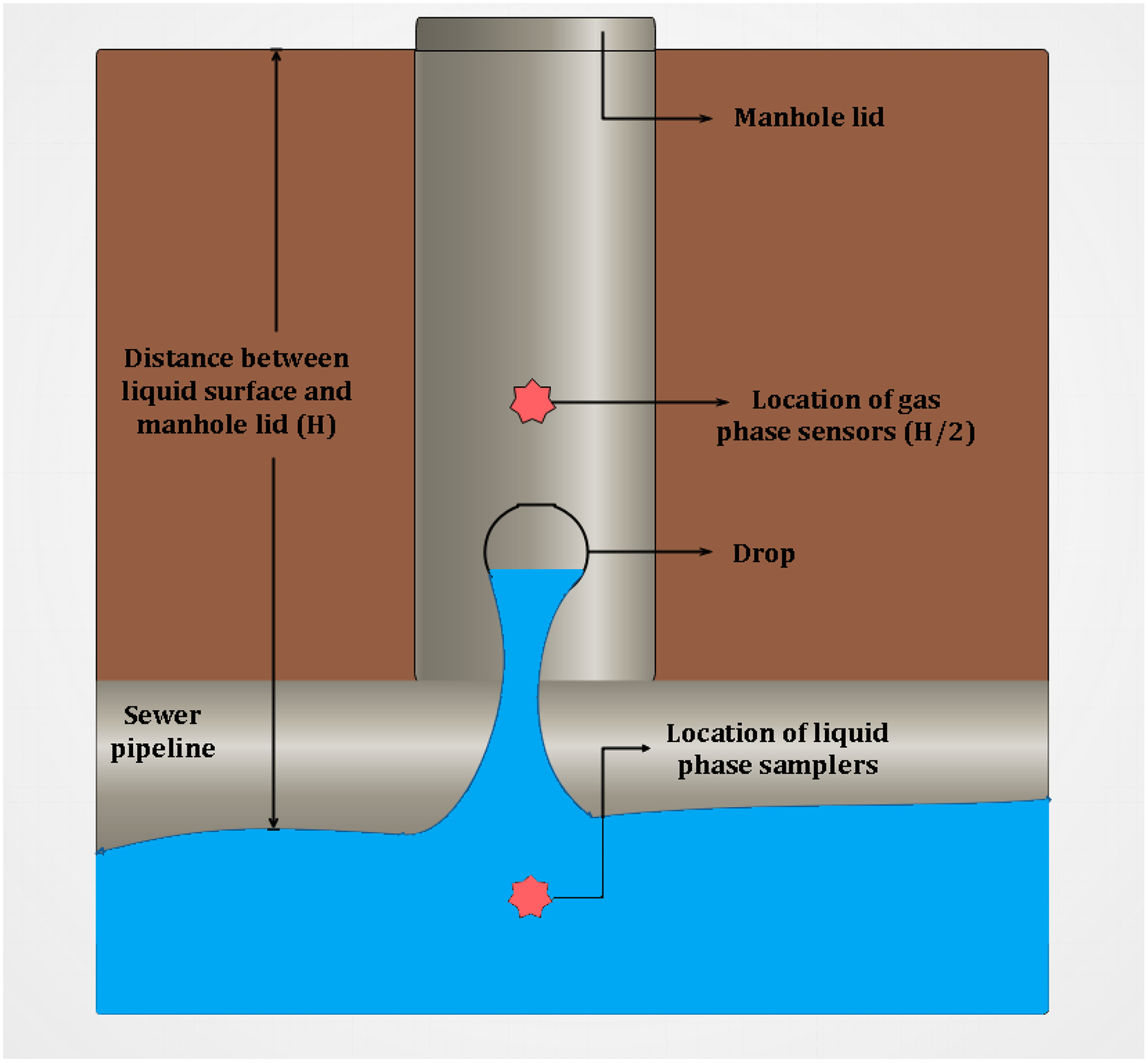
Liquid- and gas-phase samples were collected and analyzed to provide new insights into the relationship between the gas-phase concentrations and sewer environmental factors. The temperature, relative humidity, oxygen, and concentration of hydrogen sulfide in the gas phase were measured in situ along with the liquid-phase parameters such as dissolved oxygen (DO), temperature, and pH. Fig. 1 illustrates the location of instruments and sensors installed in the manhole to collect the liquid-phase samples and gas-phase data.
Monitoring equipment was deployed at a location for 48 h. For most parameters, the data were collected every minute for 48 h to understand its variation over time. The liquid samples were collected using an ISCO 6712 every hour. The changes in the liquid sample were measured on an hourly basis as the variation in liquid phase was relatively slower compared to the gas phase. The gas-phase oxygen concentration was initially measured every minute for 48 h, but the oxygen meters were extremely sensitive and could not tolerate the harsh environment inside the manhole. There were several instances where the instrument stopped working after a few hours due to the toxic environment. The trends obtained from manholes that were measured for 48 h showed that the oxygen concentration remained constant throughout the sampling period. Hence, the measurement period was reduced to 20 min. Laboratory analysis of water samples included biochemical oxygen demand () (EPA Standard Method 5210B) (Rice et al. 2012), sulfate (Method 9038 1996), and soluble and insoluble sulfide (Method 9034 1996). Slopes of the sewer system segments, velocity, and turbulence values were provided by the city. Several manholes were resampled in each season to study the seasonal variation of the liquid- and gas-phase parameters. Table 2 lists the instruments used to measure each parameter along with the frequency of measurement.
| Category | Specific parameters | Measuring instruments/method/accuracy | Frequency of measurement |
|---|---|---|---|
| Gas phase | Hydrogen sulfide () (midway between the liquid surface and the top of the manhole shaft) | OdaLog SL 1000 or Odalog SL 50 (App-Tek International) | Every minute for 48 h |
| (0–50 ppm) | |||
| Relative humidity | Kestrel DROP D2 | Every minute for 48 h | |
| 2% | |||
| Temperature | Odalog SL 50, (N/A) | Every minute for 48 h | |
| Kestrel DROP D2 | |||
| 0.9 °F | |||
| Oxygen | ToxiRAE Pro | First 20 min only | |
| (N/A) | |||
| Liquid phase | Temperature | Aqua TROLL 600 Sonde () | Every minute for 48 h |
| pH | Hanna Probe HI7698194 () | ||
| Dissolved oxygen (DO) | |||
| Biochemical oxygen demand (), dissolved | ISCO 6712 Sampler to collect sample/lab analysis using standard method 5210 B | Every hour for 48 h | |
| Sulfide, total and dissolved | ISCO 6712 sampler to collect sample/lab analysis | Every hour for 48 h | |
| EPA method 9034: titrimetric procedure | |||
| Sulfate | ISCO 6712 sampler to collect sample/lab analysis using 10227 spectrophotometer | Every hour for 48 h | |
| Velocity | Obtained from city—most values were modeled | Every 5 min for 24 h |
Results and Discussion
Hourly Variation of Liquid- and Gas-Phase Parameters
Sewage generated in a residential area is largely influenced by the lifestyle of its residents. For instance, an area where residents cook food at home tends to have more food scraps entering the sewage stream. Similarly, areas where residents prefer hair washing during the night will have sulfide-containing shampoo and other toiletry products entering the stream during the night (Matus et al. 2019). The following section will explain the general trends and the most likely reason for hourly variation of factors such as flow velocity, concentration, liquid- and gas-phase temperatures, liquid phase pH, dissolved oxygen, and relative humidity in a manhole.
Volumetric Flow
The City of Arlington provided the modeled volumetric flow rate at 5-min intervals over a 24-h period inside all monitored manholes. Fig. 2 shows examples of the hourly flow volume trend for three different manholes.
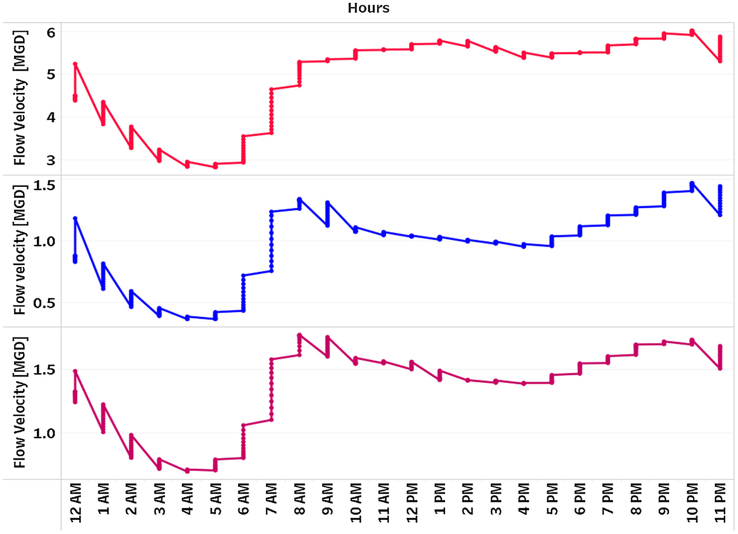
As observed in previous studies, the sewage flows were low overnight (10 p.m. to 8 a.m., with a minimum from 3 to 5 a.m.) and had peaks prior to and after normal working hours. The wastewater generated contains urine, feces, toilet paper from toilet flushing, and soap residues from the morning showers, which are generally high in sulfate and organic content. A previous study suggests that around 38% of the sulfate in sewage originates from human or industrial waste discharge (Pikaar et al. 2014). During the daytime (10 a.m. to 5 p.m.), when people are mostly away from home, the flow volume in the sewer pipes is found to be moderate. The sulfate and proteins in the sewage probably begin to break down and produce hydrogen sulfide in the wastewater, leading to build-up of the sulfide ions, hydrosulfide, and hydrogen sulfide gas while the flow velocity is lower than morning hours. In the evening when most people are back home, it is assumed that household activities such as cooking, using washing machines and dish washers, showers, baths, and hand washing are resumed, resulting in increased flow velocity from 5 p.m. to 10 p.m. After 10 p.m. the flow volume is found to decrease due to reduced human activities. A similar trend is observed for all the manholes studied, although the value of flow velocity might vary depending on the location of the sewer line.
Fig. 3 shows an example for a representative manhole and the hourly variation of factors that were measured continuously for at least 48 h. While concentration and liquid- and gas-phase temperatures follow a similar trend, liquid-phase pH follows an inverse trend. While relative humidity stayed constant throughout the period, the dissolved oxygen concentration showed a slight increase during the morning hours, when the flow velocity first peaked.
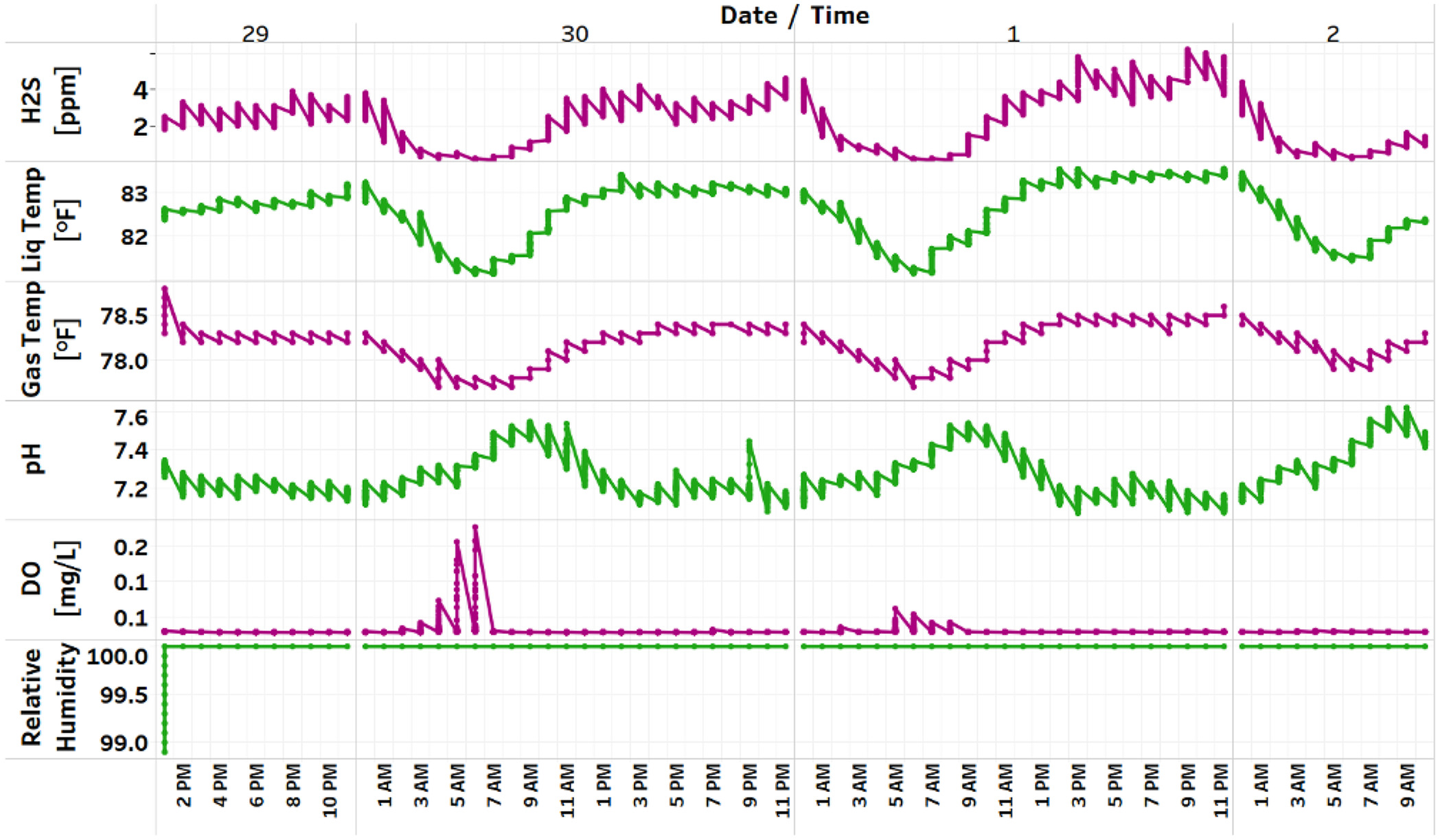
Concentration
The gas-phase concentration inside manhole follows a trend similar to the flow velocity, but with hourly offsets. In Fig. 3, while the concentration shows a declining trend in early hours of the day, the concentration steadily increases after 7 a.m. and peaks around 3 p.m. The concentration shows a slight decline after 3 p.m., and then increases to reach the maximum concentration by midnight.
The concentration of gas in the sewer system declines when the rate of volatilization of from the liquid phase is reduced. Lower flow velocity during 2–5 a.m. resulting from reduced household activities leads to lower turbulence in the sewer pipes, which increases the organic solid deposition in the pipelines, depleting oxygen and thus enhancing the growth of sulfate-reducing bacteria. However, in the early hours of the day, the available organic and sulfate content in the liquid phase is extremely low, which reduces the probability of sulfide generation in the liquid phase. This is evident from the hourly trend of gas in the manhole’s headspace from 2 a.m. to 5 a.m., where the concentration measured shows a declining trend. The trend is repeated for each consecutive day, during which the measurements were taken. The gas-phase concentration remains low even after 5 a.m., when the household activities begin and sulfate, which is naturally present in domestic water, enters the sanitary sewer system, along with human excreta and sulfur-containing soap or toiletry products. Anaerobic conditions are essential to prompt the bacteria to reduce sulfate to sulfide (Hao et al. 1996). However, increased flow velocity enhances the turbulence, causing reaeration of the wastewater, thus reducing the sulfide generation rate. Lower sulfide concentrations in the wastewater will reduce the amount of volatilized to the manhole’s headspace. Although a slight increase in gas concentration is observed, the hourly values obtained during consecutive days of sampling were lower during 5–10 a.m. Volatilization of is also temperature dependent; low liquid- and gas-phase temperature during 2–10 a.m. is also likely to be a factor, causing the low concentrations of gas in the gas phase of the manhole’s headspace.
The retention time of grit and organic solid waste that entered the sewer during early hours of the day is increased due to the reduction in the flow velocity during the daytime (10 a.m. to 6 p.m.). Reduced flow velocity limits the DO in sewer system and allows the growth of a thick slime layer, where the anaerobic bacteria reside (Grengg et al. 2015). The microbial reduction of sulfate occurs mainly in the biofilm inside sewer pipe (Nielsen and Hvitved-Jacobsen 1988). High ambient temperatures and low DO in sewage simulate the anaerobic bacteria to reduce sulfate and oxidize the organic matter, thereby increasing the concentration in the liquid phase. The acid byproducts of oxidation will reduce the wastewater pH, which significantly contributes to the dissociation of hydrogen sulfide in liquid phase to hydrogen sulfide gas (), hydrosulfide ion (), and sulfide ion (). When the pH falls from neutral (7) to slightly acidic (6), hydrogen sulfide dissociates to 90% dissolved hydrogen sulfide gas and 10% hydrosulfide ion (USEPA 1992). Volatilization of increases with the decrease in the pH (ASCE 1995), and this explains the cause of recording high concentrations in the manhole from 10 a.m. to 6 p.m. However, due to calmer flow, the rate of volatilization is reduced, and most of the generated is still present in the wastewater and is available for volatilization. After 6 p.m. the flow velocity increases, and volatilization induced by the turbulence strips the in wastewater to the headspace of the manhole. This explains the high concentration measured in the sewer atmosphere after 8 p.m., and the peaking observed around midnight. This general trend is observed in all the manholes during the consecutive days in which the study was conducted.
Liquid and Gas Temperature
The liquid- and gas-phase temperatures in Fig. 3 show a declining trend in the early hours of the day and record minimum values during 5–7 a.m. Temperature inside the manhole increases after 7 a.m. and peaks around 1 p.m. The temperature remains almost stagnant until midnight and then begins to drop, reaching the lowest temperature around 5 a.m. on the following day. In all the manholes studied, the gas-phase temperature inside the manhole was found to be lower than the liquid-phase temperature. Although the range of temperatures might vary in different seasons, the general hourly trend was observed to be similar in both liquid- and gas-phase temperatures. The seasonal variations of the liquid and gas temperature is discussed in detail in the section titled ‘Relationship between liquid-phase temperature and gas-phase temperature’.
The low ambient temperature and reduced hot water usage during the early hours (12–5 a.m.) of the day results in low liquid- and gas-phase temperatures inside a manhole. After 6 a.m., increased use of warm water for daily cleansing increases the liquid-phase temperature, and the rise in ambient temperature increases the gas-phase temperature in manholes. Although the hot water usage reduces after 10 a.m., the increase in external temperature and the exothermic reactions due to increased microbial activity in the anaerobic sewer conditions results in elevated liquid and gas temperature from 11 a.m. to 7 p.m. Both the temperatures were found to peak around 1 p.m., when ambient temperature was highest, implying that the temperature inside a manhole is influenced by changes in wastewater temperature and ambient weather conditions. After 7 p.m., though the temperature outside the manhole begins to fall, the increased warm water usage in households results in elevated liquid-phase temperatures. The exothermic reaction, which results in the generation of gas after 8 p.m., also results in increased liquid temperature, which also increases gas-phase temperature at night.
Liquid-Phase pH
From Fig. 3 the hourly variation of pH follows an inverse trend compared to that of concentration, liquid-phase temperature, and gas-phase temperature recorded inside a manhole. The pH shows an increasing trend post 2 a.m. and reaches a peak between 7 and 10 a.m. The pH starts to fall after 10 a.m., and the minimum reading is observed around 3 p.m., which then continues to remain at the same level until 1 a.m. the following day. We observed sewage pH values within the normal range of 5.5 to 8.0 (Sharma et al. 2013) the maximums observed between 5 and 10 a.m. Toiletry products are generally alkaline, varying from pH 8 to 13. The pH is found to follow a decreasing trend after 10 a.m. and reaches a minimum value around 3 p.m., which is continued until 1 a.m. the following day. This could be influenced by the anaerobic decomposition of organic matter in the sewer system, which generates acid byproducts that reduce pH.
Dissolved Oxygen and Relative Humidity
The hourly variation of dissolved oxygen and relative humidity inside a manhole is plotted in Fig. 3, continuously for more than 48 h. The hourly variation of the DO in wastewater follows an inverse trend in comparison with the concentration. The DO concentration slightly increases to when higher flow velocity causes turbulence and adds oxygen to the sewage. This is evident from the hourly trend of DO in Fig. 3, where the concentration slightly increases during 5–10 a.m., with the peak around 6–7 a.m. According to Henry’s law, the solubility of gas decreases with an increase in temperature, leading to lower DO concentration during the daytime. The presence of electrolytes is found to reduce the solubility of oxygen (Xing et al. 2014), and in sanitary sewage high concentrations of chloride and sodium due to the human diet and composition of cleaning products could decrease DO (de Almeida et al. 2015). During the study several manholes recorded the DO concentration to be zero during the day, and in some manholes DO measurements were not recorded. This could be because the DO level was below the instrument’s ability to detect.
Low relative humidity values were recorded inside the manholes for the initial hours post installation of instruments. This was due to the interaction of air inside and outside of the manhole as the manhole lid was opened for equipment installation. After an initial decrease, the relative humidity remained at 100% most of the time. The concentration of relative humidity increased in a few cases with gas temperature and decreased in other cases. This unexplained variability in the relative humidity data could possibly be due to various design characteristics and flow conditions in a manhole. Manhole depth or presence of multiple inlets in a manhole changes the moisture content in the manhole, thus causing relative humidity to vary. Further analysis is required to draw any conclusions.
Impact of Gas- and Liquid-Phase Parameters on Liquid-Phase Hydrogen Sulfide Generation and Volatilization to Gas Phase
The factors contributing to generation and volatilization of and their levels leading to these processes are listed in Table 3. Although the relation between all the parameters in Table 2 were explored, only the factors listed in Table 4 showed weak linear correlation with the measured variables. Other parameters explored exhibited very weak correlation, probably be due to the interdependence of multiple factors such as wastewater characteristics, manhole design, and flow conditions. Weather conditions, especially temperature, could also have affected these variables, as some decent correlations were observed for variables of manholes sampled during the summer season.
| Process examined | Parameter | Level leading to formation | Reference |
|---|---|---|---|
| Level leading to formation | DO | ASCE (1989) | |
| BOD | ASCE (2007) | ||
| Sulfate | Higher the sulfate level, the greater the formation | ASCE (1995) | |
| Temperature | Generally | ASCE (2009) | |
| Flow velocity | Rule of thumb: for pipe flowing fulla | ASCE (1989) | |
| Slope | Low | USEPA (1992) | |
| Turbulence | Low | ASCE (1989) | |
| Level leading to volatilization | Liquid-phase concentration | or lower (dissolved) | USEPA (1992) |
| Turbulence | High | ASCE (1989) | |
| Slope | High | ASCE (1989) | |
| Flow velocity | High | ASCE (1989) | |
| Temperature | High | ASCE (1989) | |
| pH | (around 90% of sulfide is in the form of at ) | USEPA (1992) |
a
Actually, it depends on BOD and flow geometry (cross-sectional area and surface width of flow).
| Process | Variables explored | Correlation | Probable reason |
|---|---|---|---|
| Generation of in wastewater | Dissolved oxygen | Inverse | At low DO levels (), the anaerobic bacteria oxidize organic matter and form sulfide. This sulfide further reacts with hydrogen in water to form hydrogen sulfide. |
| Sulfate | Direct | High concentrations of sulfate released by the hydrolysis of sulfur-bearing proteins in sewage serves as the food for sulfate reducing-bacteria, leading to higher concentrations. | |
| Temperature | Direct | As temperature increases, the bacterial activity will increase, resulting in a rise in concentrations. | |
| Volatilization of | pH | Inverse | As the pH increases, in liquid phase dissociates to hydrosulfide ion () and sulfide ion (). |
| Temperature | Direct | As temperature increases, volatilization of the dissolved gas increases in accordance with Henry’s law. | |
| Sulfide | Inverse | Dissolved hydrogen sulfide is the only form of sulfide that can be released from wastewater to the atmosphere as gas. The higher the concentration of in the liquid phase, the higher the rate of volatilization. |
Impact of Manhole Category on Gas-Phase Hydrogen Sulfide Concentration
Manholes can be categorized based on their physical designs such as the presence or absence of drop, height of drop, type of flow, number of inlets flowing into the manhole, diameter of upstream and downstream pipes, and presence or absence of bends. These physical designs will dictate the amount of hydrogen sulfide that will be volatilized to the manhole’s headspace. Fig. 4 shows the average concentration observed in manholes with different design categories. Manholes with hydraulic jump recorded the highest average reading, followed by the ones with bends and drop . The lowest concentration of was observed in manholes with a standard drop of , followed by manholes with uniform pipe diameter upstream and downstream.

Drop
A drop is a structural element inside a manhole that guides the flow and allows free fall of sewage from a shallow upstream pipe to a deeper downstream pipe in a sanitary sewer line. The sudden drop during the flow creates turbulence, causing the stripping of from the liquid to gas phase. Drops can be classified in to three categories depending on the depth or height of drops: drop height , drop height between and , and standard drop height of . As observed in Fig. 4, the highest average concentration was observed in manholes with drops greater than . Higher drops induce a higher rate of volatilization of from liquid to gas phase due to enhanced turbulence. The average concentration demonstrates a declining trend as the height of drop decreases.
Pipe Diameter
The sewer pipeline diameter is chosen, considering factors such as flow volume and slope, to attain a flow velocity that minimizes the settling of grit and organic solids. Depending on the diameter of the upstream and downstream pipes of a manhole, three distinct categories can be found in the sanitary sewer system: uniform diameter, diameter changing from smaller to larger, and diameter changing from larger to smaller size. Fig. 4 shows that manholes with pipelines having uniform diameter both upstream and downstream exhibited the lowest concentration due to least disturbance generated during the transition from upstream to downstream sewer line. The highest gas concentration was observed when the flow entered a smaller pipeline from a larger one. The sudden reduction in the diameter and surface area enhances the flow velocity and turbulence, thereby increasing the rate of volatilization. When the flow enters a larger pipe from a smaller pipe, the change in diameter causes turbulence. As a result, the concentration here is higher than the pipes with uniform diameter but lower than the pipes with larger pipe upstream and smaller pipe downstream. As a result, the concentration here is higher than the pipes with uniform diameter but lower than the pipes with larger pipe upstream and smaller pipe downstream.
Flow Category
The sewer system takes advantage of gravity flow by placing the pipes in a slight gradient to transport wastewater from the point of generation to the sewage treatment facilities. Gravity sewers are generally designed to maintain subcritical flow conditions (low velocity, high depth of flow, and small bottom slope) in the pipeline to reduce turbulence, which causes volatilization. However, due to natural topography and ground conditions, supercritical flow (high velocity, low depth of flow, and steep bottom slope) might be inevitable. In this study, manholes with three distinct flow categories were considered in the sanitary sewer system: supercritical flow both upstream and downstream, subcritical flow both upstream and downstream, and supercritical flow upstream/subcritical flow downstream, which is also called a hydraulic jump. As shown in Fig. 4, the highest concentration of was observed for hydraulic jumps. The hydraulic jump creates zones of high turbulence due to the sudden change in flow, leading to stripping from liquid to gas phase.
Due to the high velocity and steeper bottom slope, manholes with supercritical flow are expected to record higher concentration of in the gas phase. However, manholes with subcritical flow upstream and downstream recorded higher values compared to ones with supercritical flow both upstream and downstream. The disparity in the number of manholes with subcritical and supercritical flows both upstream and downstream could have affected the average value of concentration, thereby causing the variation. Additionally, several manholes in the subcritical flow category recorded very high concentration of , probably due to other nonstructural factors such as wastewater characteristics and seasonal variation. Further investigation is required to draw a clear conclusion.
Bends and Multiple Inlets
Manholes with bends produce high concentration in the headspace, as can be clearly inferred from Fig. 4, as this category is preceded only by one category. Bends are used in sewer pipelines to guide the flow when a change in the flow direction is essential. Depending on the angles at which the upstream and downstream pipes are laid, bends can have different angles. Manholes with a wide range of bends, varying from 90° to 170°, were observed during our investigation. Sharp bends are sources of turbulence leading to stripping of from liquid to gas phase in the sewer system.
Similarly, multiple inlets in a manhole lead to collision of wastewater from different inlets, generating higher turbulence and volatilization at the point of contact. The average concentration for manholes with multiple inlets is less than bends but remarkably high compared to the control manhole. Control manholes have uniform diameter and a single inlet with no drops or bends. The average concentration in control manholes was 0.97 ppm, which was slightly higher than manholes with uniform pipe diameter. This could be because the control manholes had subcritical flow, which recorded higher than supercritical flow.
Impact of Season on Hydrogen Sulfide Concentration
To study the seasonal variation of concentration in the manholes, a set of 10 manholes was selected, and the liquid- and gas-phase parameters were measured in three time periods: winter/spring (January–May), summer (June–August), and fall/winter (September–December). Fig. 5 shows the variation in liquid temperature and concentration for the same manhole during three seasons. The parameters were measured for more than 60 h during each season.

Ambient temperature was the main external parameter that varied during each season. In the manholes studied for seasonal variation, concentration inside manholes increased as the temperature rose. Summer recorded the highest temperature among the seasons, followed by fall and spring. The highest concentration was also recorded in summer for all the manholes studied, suggesting that higher liquid temperature resulted in increased bacterial activity and generated higher concentrations of in manholes.
Table 5 shows the variation of average sulfate and sulfide in the liquid phase, BOD, temperature, and average hydrogen sulfide concentration for the representative manhole presented in Fig. 5, during different seasons. For domestic wastewater, the main source of sulfur is sulfate () in a concentration range of (Zhang et al. 2008). At higher temperature the sulfate is reduced to sulfide by the sulfate-reducing bacteria while anaerobic conditions prevail, and then the is emitted as hydrogen sulfide to sewer atmosphere depending on temperature, pH, and hydraulic conditions. From the data in Table 5, the average readings in summer clearly show that most of the sulfate is converted to sulfide and volatilized to , exhibiting a higher average concentration in the manhole headspace. However, in fall, even with temperature higher, the average sulfate and sulfide content in liquid phase remained higher than spring. The change in waste composition, which is evident from the average BOD measurements, could be the probable reason for this. A previous study reported that the oxidation rate of sulfide doubled when the temperature increased by 7–9°C (Jiang et al. 2014). The high concentration of hydrogen sulfide observed in manhole headspace for all the manholes studied for seasonal variation during summer aligns with this result.
| Season | Sulfate, | Sulfide, | , ppm | Temperature, °F | BOD | |||||
|---|---|---|---|---|---|---|---|---|---|---|
| Mean | Standard deviation | Mean | Standard deviation | Mean | Standard deviation | Mean | Standard deviation | Mean | Standard deviation | |
| Winter/spring (January–May) | 66.395 | 15.103 | 26.038 | 12.934 | 0.595 | 0.248 | 63.503 | 2.042 | 303.902 | 375.549 |
| Summer (June–August) | 51.469 | 32.316 | 39.604 | 18.500 | 2.059 | 1.846 | 80.176 | 5.305 | 145.046 | 115.533 |
| Fall/winter (September–December) | 59.558 | 26.936 | 38.926 | 18.798 | 0.600 | 0.839 | 72.050 | 7.788 | 221.938 | 110.170 |
Relationship between Liquid-Phase Temperature and Gas-Phase Temperature
While studying the seasonal variation of liquid- and gas-phase parameters, the average liquid- and gas-phase temperatures in the manhole were found follow a similar pattern during the three seasons. The average temperature in liquid and gas phase inside manhole and their difference for the three seasons are tabulated in Table 6.
| Season | Average liquid-phase temperature (°F) | Average gas-phase temperature (°F) | Variation between average liquid-phase and average gas-phase temperature |
|---|---|---|---|
| Fall/winter 2017 | 78.130 | 76.052 | 2.078 |
| Winter/spring 2018 | 68.148 | 61.897 | 6.251 |
| Summer 2018 | 81.535 | 80.897 | 0.638 |
| Fall/winter 2018 | 78.832 | 76.978 | 1.854 |
The spring season recorded the lowest temperature, and summer recorded the highest temperature in both liquid and gas phase. The temperature difference in the gas and liquid phase also followed the same trend. The average liquid-phase temperature always exceeded the gas-phase temperature inside a manhole. On average, the liquid- and gas-phase temperature inside the manhole varied by 3° in all three seasons studied. The result of the study was in line with a previous study by Romanova et al. (2014), where the average liquid-phase temperature was found to be higher by 3.5°F when two manholes were studied for a period of two months. In the current study, the maximum difference was 6°F in spring due to the colder atmospheric temperature outside the manhole, and the minimum average difference was 0.6°F in summer because of higher atmospheric temperature outside the manhole. The fall of 2018 had fewer data points compared to the fall of 2017, which could potentially be a reason for the slight reduction in the temperature variance in liquid and gas phases.
Conclusions and Future Recommendations
The corrosion of manholes is one of the most challenging problems regarding sewer operation and maintenance for many cities. Multiple factors are involved in generation and volatilization of hydrogen sulfide, causing corrosion of manholes. This study aimed to investigate the linear relation between various factors affecting generation and volatilization from liquid to gas phase.
1.
concentration, liquid-phase temperature, and liquid-phase pH in some cases showed similar hourly trends in consecutive days of sampling. The trend in rise and fall of concentration of these parameters over time showed slight variations depending on the manhole’s location and category.
2.
No strong linear relation was found between liquid-/gas-phase parameters and hydrogen sulfide generation and volatilization to gas phase. This could be due to the involvement of multiple parameters simultaneously for the generation and volatilization of .
3.
The manhole categories play a significant role in generation. The manholes with hydraulic jump generated the highest average concentration, followed by manholes with drops. The lowest concentration of was observed in manholes with subcritical flow upstream and downstream. This was followed by manholes with uniform pipe diameter upstream and downstream.
4.
In all the manholes studied for seasonal variation, the concentration of hydrogen sulfide was found to be maximum during the summer, when the temperature was highest among the three seasons.
5.
The average liquid-phase temperature is always greater than the ambient temperature inside a manhole. In the three seasons considered (spring, summer, and fall), the liquid-phase temperature and ambient temperature inside manhole varies by 3°F on an average.
Recommendations for future research include the following:
1.
Further research is necessary to determine the effects of seasonal variations on the gas- and liquid-phase parameters in a manhole. Instead of combining fall–winter and winter–spring, sampling in these seasons separately might help to give us a better understanding of seasonal variations.
2.
To better understand the correlations and contribution of each predictor variable, multiple linear regression (MLR) or advanced machine learning techniques could be employed.
3.
In future studies measuring the redox potential could explain the oxidizing capacity of sewage.
Data Availability Statement
The data collected from the site ( concentration, relative humidity, temperature, pH, dissolved oxygen, manhole features and categories) and data obtained from laboratory analysis (BOD, sulfide—total and dissolved, sulfate) that support the findings of this study will be available from the corresponding author upon reasonable request. Volumetric flow data were provided by the City of Arlington, and direct requests for these materials may be made to the provider.
Acknowledgments
The authors acknowledge the City of Arlington for funding the project (Award No. 1268202901) and training the research team to access the manholes. The authors also acknowledge the following graduate and undergraduate members of SEER laboratory: Sunita Baniya, Mithila Chakraborty, Mateo Galvez, Gomathy Radhakrishna Iyer, Jacob Kim, Rafatuzzama Mohammad, Samir Nathu, Niloofar Parsaeifard, Hoda Rahimi, Ketan Shah, Ankita Sinha, Tyler Terashima, and Natasha Wooten.
References
ASCE. 1989. Sulfide in wastewater collection and treatment systems. Reston, VA: ASCE.
ASCE. 1995. Odor control in wastewater treatment plants. Reston, VA: ASCE.
ASCE. 2007. Gravity sanitary sewer design and construction, second edition. Reston, VA: ASCE.
ASCE. 2009. Manhole inspection and rehabilitation. 2nd ed. Reston, VA: ASCE.
Berndt, M. L. 2011. “Evaluation of coatings, mortars and mix design for protection of concrete against sulphur oxidising bacteria.” Constr. Build. Mater. 25 (10): 3893–3902. https://doi.org/10.1016/j.conbuildmat.2011.04.014.
de Almeida, M., F. Vargas-Zerwes, L. Ferreira-Bastos, A. Ben da Costa, R. de Souza-Schneider, Ê. L. Machado, and A. Kohler. 2015. “Cation and anion monitoring in a wastewater treatment pilot project.” Rev. Facultad de Ing. Universidad de Antioquia 2015 (76): 82–89. https://doi.org/10.17533/UDEA.REDIN.N76A10.
de Muynck, W., N. de Belie, and W. Verstraete. 2009. “Effectiveness of admixtures, surface treatments and antimicrobial compounds against biogenic sulfuric acid corrosion of concrete.” Cem. Concr. Compos. 31 (3): 163–170. https://doi.org/10.1016/j.cemconcomp.2008.12.004.
Ganigue, R., O. Gutierrez, R. Rootsey, and Z. Yuan. 2011. “Chemical dosing for sulfide control in Australia: An industry survey.” Water Res. 45 (19): 6564–6574. https://doi.org/10.1016/j.watres.2011.09.054.
Grengg, C., F. Mittermayr, A. Baldermann, M. E. Böttcher, A. Leis, G. Koraimann, P. Grunert, and M. Dietzel. 2015. “Microbiologically induced concrete corrosion: A case study from a combined sewer network.” Cem. Concr. Res. 77 (Nov): 16–25. https://doi.org/10.1016/j.cemconres.2015.06.011.
Haile, T., and G. Nakhla. 2010. “The inhibitory effect of antimicrobial zeolite on the biofilm of Acidithiobacillus thiooxidans.” Biodegradation 21 (1): 123–134. https://doi.org/10.1007/s10532-009-9287-6.
Hao, O. J., J. M. Chen, L. Huang, and R. L. Buglass. 1996. “Sulfate-reducing bacteria.” Crit. Rev. Environ. Sci. Technol. 26 (2): 155–187. https://doi.org/10.1080/10643389609388489.
Jensen, H. S., A. H. Nielsen, P. N. L. Lens, T. Hvitved-Jacobsen, and J. Vollertsen. 2009. “Hydrogen sulphide removal from corroding concrete: Comparison between surface removal rates and biomass activity.” Environ. Technol. 30 (12): 1291–1296. https://doi.org/10.1080/09593330902894356.
Jiang, G., O. Gutierrez, K. R. Sharma, J. Keller, and Z. Yuan. 2011. “Optimization of intermittent, simultaneous dosage of nitrite and hydrochloric acid to control sulfide and methane productions in sewers.” Water Res. 45 (18): 6163–6172. https://doi.org/10.1016/j.watres.2011.09.009.
Jiang, G., D. Melder, J. Keller, and Z. Yuan. 2017. “Odor emissions from domestic wastewater: A review.” Rev. Environ. Sci. Technol. 47 (17): 1581–1611. https://doi.org/10.1080/10643389.2017.1386952.
Jiang, G., K. R. Sharma, and Z. Yuan. 2013. “Effects of nitrate dosing on methanogenic activity in a sulfide-producing sewer biofilm reactor.” Water Res. 47 (5): 1783–1792. https://doi.org/10.1016/j.watres.2012.12.036.
Jiang, G., J. Sun, K. R. Sharma, and Z. Yuan. 2015. “Corrosion and odor management in sewer systems.” Curr. Opin. Biotechnol. 33 (Jun): 192–197. https://doi.org/10.1016/j.copbio.2015.03.007.
Jiang, G., E. Wightman, B. C. Donose, Z. Yuan, P. L. Bond, and J. Keller. 2014. “The role of iron in sulfide induced corrosion of sewer concrete.” Water Res. 49 (Feb): 166–174. https://doi.org/10.1016/j.watres.2013.11.007.
Jiang, G., and Z. Yuan. 2013. “Synergistic inactivation of anaerobic wastewater biofilm by free nitrous acid and hydrogen peroxide.” J. Hazard. Mater. 250 (Apr): 91–98. https://doi.org/10.1016/J.JHAZMAT.2013.01.047.
Kaushal, V., M. Najafi, and J. Love. 2018. “Qualitative investigation of microbially induced corrosion of concrete in sanitary sewer pipe and manholes.” Pipelines 2018 (Jul): 768–775. https://doi.org/10.1061/9780784481653.086.
Koch, G. H., M. P. H. Brongers, N. G. Thompson, Y. P. Virmani, and J. H. Payer. 2002. Corrosion cost and preventive strategies in the United States. Washington, DC: Federal Highway Administration.
Lebrero, R., L. Bouchy, R. Stuetz, and R. Muñoz. 2011. “Odor assessment and management in wastewater treatment plants: A review.” Crit. Rev. Environ. Sci. Technol. 41 (10): 915–950. https://doi.org/10.1080/10643380903300000.
Li, X., P. L. Bond, L. O’moore, S. Wilkie, L. Hanzic, I. Johnson, K. Mueller, Z. Yuan, and G. Jiang. 2020. “Increased resistance of nitrite-admixed concrete to microbially induced corrosion in real sewers.” Environ. Sci. Technol. 54 (4): 2323–2333. https://doi.org/10.1021/acs.est.9b06680.
Li, X., L. O’Moore, Y. Song, P. L. Bond, Z. Yuan, S. Wilkie, L. Hanzic, and G. Jiang. 2019. “The rapid chemically induced corrosion of concrete sewers at high H2S concentration.” Water Res. 162 (Oct): 95–104. https://doi.org/10.1016/j.watres.2019.06.062.
Matus, M., C. Duvallet, M. Soule, S. Kearney, N. Endo, N. Ghaeli, I. Brito, C. Ratti, E. Kujawinski, and E. Alm. 2019. “24-hour multi-omics analysis of residential sewage reflects human activity and informs public health.” bioRxiv 728022. https://doi.org/10.1101/728022.
Method 9034. 1996. Titrimetric procedure for acid-soluble and acid-insoluble sulfides. Washington, DC: USEPA.
Method 9038. 1996. Acid-soluble and acid-insoluble sulfides: Distillation. Washington, DC: USEPA.
Nielsen, P. H., and T. Hvitved-Jacobsen. 1988. “Effect of sulfate and organic matter on the hydrogen sulfide formation in biofilms of filled sanitary sewers.” Journal (Water Pollution Control Federation) 60 (5): 627–634.
O’Connell, M., C. McNally, and M. G. Richardson. 2010. “Biochemical attack on concrete in wastewater applications: A state of the art review.” Cem. Concr. Compos. 32 (7): 479–485. https://doi.org/10.1016/j.cemconcomp.2010.05.001.
Parande, A. K., P. L. Ramsamy, S. Ethirajan, C. R. K. Rao, and N. Palanisamy. 2006. “Deterioration of reinforced concrete in sewer environments.” Proc. Inst. Civ. Eng. Munic. Eng. 159 (Mar): 11–20. https://doi.org/10.1680/muen.2006.159.1.11.
Parker, C. D. 1945. “The corrosion of concrete: 1. The isolation of a species of bacterium associated with the corrosion of concrete exposed to atmospheres containing hydrogen sulphide.” Aust. J. Exp. Biol. Med. Sci. 23 (2): 81–90. https://doi.org/10.1038/icb.1945.13.
Parker, C. D. 1947. “Species of sulphur bacteria associated with the corrosion of concrete.” Nature 159 (4039): 439–440. https://doi.org/10.1038/159439b0.
Parker, C. D. 1951. “Mechanics of corrosion of concrete sewers by hydrogen sulfide.” Sewage Ind. Wastes 23 (12): 1477–1485.
Pikaar, I., K. R. Sharma, S. Hu, W. Gernjak, J. Keller, and Z. Yuan. 2014. “Reducing sewer corrosion through integrated urban water management.” Science 345 (6198): 812–814. https://doi.org/10.1126/science.1251418.
Rice, E. W., R. B. Baird, A. D. Eaton, and L. S. Clesceri. 2012. Standard methods for the examination of water and wastewater. Washington, DC: American Public Health Association.
Roberts, D. J., D. Nica, G. Zuo, and J. L. Davis. 2002. “Quantifying microbially induced deterioration of concrete: Initial Studies.” Int. Biodeterior. Biodegrad. 49 (4): 227–234. https://doi.org/10.1016/S0964-8305(02)00049-5.
Romanova, A., M. Mahmoodian, and A. Alani. 2014. “Influence and interaction of temperature, H2S and pH on concrete sewer pipe corrosion.” Int. J. Civ. Environ. Struct. Constr. Archit. Eng. 8 (6): 621–624.
Saraswathy, V., and H. W. Song. 2007. “Corrosion performance of rice husk ash blended concrete.” Constr. Build. Mater. 21 (8): 1779–1784. https://doi.org/10.1016/j.conbuildmat.2006.05.037.
Sharma, K., R. Ganigue, and Z. Yuan. 2013. “pH dynamics in sewers and its modeling.” Water Res. 47 (16): 6086–6096. https://doi.org/10.1016/j.watres.2013.07.027.
Song, Y., et al. 2021. “A novel granular sludge-based and highly corrosion-resistant bio-concrete in sewers.” Sci. Total Environ. 791 (Oct): 148270. https://doi.org/10.1016/j.scitotenv.2021.148270.
Sun, X., G. Jiang, P. L. Bond, J. Keller, and Z. Yuan. 2015. “A novel and simple treatment for control of sulfide induced sewer concrete corrosion using free nitrous acid.” Water Res. 70 (Mar): 279–287. https://doi.org/10.1016/j.watres.2014.12.020.
USEPA. 1991. Hydrogen sulfide corrosion in wastewater collection and treatment systems. Washington, DC: USEPA.
USEPA. 1992. Detection, control, and correction of hydrogen sulfide corrosion in existing wastewater systems. EPA 832-R-92-001. Washington, DC: USEPA.
Wang, X., G. Parcsi, J. Cesca, E. Sivret, and R. Stuetz. 2010. “Olfactory characterisation of NMVOC emissions from WWTP inlet works.” Water 37 (Mar): 82–86.
Wei, S., M. Sanchez, D. Trejo, and C. Gillis. 2010. “Microbial mediated deterioration of reinforced concrete structures.” Int. Biodeterior. Biodegrad. 64 (8): 748–754. https://doi.org/10.1016/j.ibiod.2010.09.001.
Wells, T., and R. E. Melchers. 2014. “An observation-based model for corrosion of concrete sewers under aggressive conditions.” Cem. Concr. Res. 61 (Jul): 1–10. https://doi.org/10.1016/j.cemconres.2014.03.013.
Wells, T., and R. E. Melchers. 2015. “Modelling concrete deterioration in sewers using theory and field observations.” Cem. Concr. Res. 77 (Nov): 82–96. https://doi.org/10.1016/j.cemconres.2015.07.003.
Xing, W., M. Yin, Q. Lv, Y. Hu, C. Liu, and J. Zhang. 2014. “Oxygen solubility, diffusion coefficient, and solution viscosity.” In Rotating electrode methods and oxygen reduction electrocatalysts, 1–31. Amsterdam, Netherlands: Elsevier. https://doi.org/10.1016/B978-0-444-63278-4.00001-X.
Zhang, L., P. De Schryver, B. De Gusseme, W. De Muynck, N. Boon, and W. Verstraete. 2008. “Chemical and biological technologies for hydrogen sulfide emission control in sewer systems: A review.” Water Res. 42 (1–2): 1–12. https://doi.org/10.1016/j.watres.2007.07.013.
Zhu, T., and M. Dittrich. 2016. “Carbonate precipitation through microbial activities in natural environment, and their potential in biotechnology: A review.” Front. Bioeng. Biotechnol. 4 (Jan): 4. https://doi.org/10.3389/FBIOE.2016.00004/BIBTEX.
Information & Authors
Information
Published In

Journal of Environmental Engineering
Volume 150 • Issue 5 • May 2024
Copyright
This work is made available under the terms of the Creative Commons Attribution 4.0 International license, https://creativecommons.org/licenses/by/4.0/.
History
Received: Apr 13, 2023
Accepted: Dec 14, 2023
Published online: Feb 24, 2024
Published in print: May 1, 2024
Discussion open until: Jul 24, 2024
ASCE Technical Topics:
- Chemical compounds
- Chemicals
- Chemistry
- Concrete
- Corrosion
- Deterioration
- Energy engineering
- Energy sources (by type)
- Engineering fundamentals
- Engineering materials (by type)
- Environmental engineering
- Fuels
- Infrastructure
- Lifeline systems
- Manholes
- Materials characterization
- Materials engineering
- Mathematics
- Microbes
- Natural gas
- Non-renewable energy
- Organisms
- Parameters (statistics)
- Petroleum
- Salts
- Sewers
- Statistics
- Sulfides
Authors
Metrics & Citations
Metrics
Citations
Download citation
If you have the appropriate software installed, you can download article citation data to the citation manager of your choice. Simply select your manager software from the list below and click Download.