Quantifying the Impact of Climate Change on Peak Stream Discharge for Watersheds of Varying Sizes in the Coastal Plain of Virginia
Publication: Journal of Hydrologic Engineering
Volume 29, Issue 3
Abstract
Civil infrastructure systems have traditionally been designed assuming stationarity in precipitation. However, climate change is making this assumption invalid, affecting both existing infrastructure designed assuming stationarity and the design of new infrastructure. Although many studies have analyzed potential increases in precipitation due to climate change, fewer have attempted to translate these changes into the impact of stream discharge in a way that could be incorporated into infrastructure design. Therefore, this study aimed to assess the potential impact of climate change on both rainfall and peak discharge to aid in bridge and road infrastructure design. Results showed that the median increase in model-derived rainfall intensity across the selected rainfall stations in Virginia was 10%–30% for the midcentury (centered on 2045) and 10%–40% for the end of the century (centered on 2085), with the higher increase for the Representative Concentration Pathway 8.5 (RCP8.5) scenario compared with the RCP4.5 scenario. A regression analysis was performed to relate peak discharge to watershed size for midcentury and end-of-century periods for the study area. In terms of peak discharge, smaller watersheds () had a percent increase for a given return period that was independent of the watershed size. Considering both RCP4.5 and RCP8.5 scenarios, for a 100-year return period, the increase was 39% and 49%, respectively, for the midcentury periods and 36% and 52%, respectively, for the end-of-century periods. For larger watersheds (), the increase in peak discharge decreased as the watershed size increased, suggesting a dampening effect for larger watersheds in this coastal plain region of Virginia. For a watershed size of , the largest watershed included in the analysis, the percent increase in peak discharge for a 100-year return period was 14% and 39% during the midcentury, and 16% and 40% at the end of the century, for the two emission scenarios. These findings and the general methodology used in the study can aid transportation and water resources engineers in incorporating changing rainfall impacts into assessing current infrastructure and designing future infrastructure. They can also help to prioritize resources for more costly hydraulic analyses of potentially vulnerable infrastructure.
Practical Applications
The study aims to understand better how climate change will impact future precipitation and how this change in precipitation will impact peak discharge for watersheds of various sizes. Using Virginia as a study region, the median increase in precipitation intensity was found to be between 10% and 30% for the midcentury and 10%–40% for the end of the century across the state. Smaller watersheds () had an increase in peak discharge for a given return period that was independent of the watershed size. In comparison, larger watersheds () had an increase in peak discharge, but the percent increase in peak discharge decreased as the size of the watershed increased, especially for the RCP8.5 emission scenario. Regression equations were developed to provide a first approximation of peak discharge based on the watershed area, the emission scenario, and the return period to aid decision-makers in the region when including climate change impacts when assessing existing or designing new hydraulic structures.
Introduction
Civil infrastructure systems have traditionally been designed assuming stationarity in precipitation records, meaning there will be no significant long-term trends in precipitation patterns, intensities, and frequencies over time (Bhatkoti et al. 2016). However, growing evidence suggests that climate change makes this nonstationarity assumption inappropriate (Milly et al. 2008). The Third National Climate Assessment (NCA) showed that heavy precipitation (i.e., downpours, the heaviest 1% of all daily events) has been increasing across the US, with particularly strong changes observed in the northeast, southeast, and Upper Mississippi River valley regions (Walsh et al. 2014). Unfortunately, most current hydraulic infrastructure (e.g., bridges and culverts), flood control infrastructure (e.g., dams, spillways, and reservoirs), and stormwater infrastructure (e.g., sewer pipes and detention basins) have been and are continuing to be designed assuming stationary climate conditions (Martel et al. 2021; Lopez-Cantu and Samaras 2018). An assumption of stationarity could cause a substantial under- or overestimation of design storms (Cheng and AghaKouchak 2014). In the case of underestimation, this could result in the insufficient design of hydraulic structures, and even loss of life and properties in the case of flooding. In the case of overestimation, structures could be overdesigned, resulting in inefficient use of limited infrastructure funding.
How nonstationary climate change should be used to design local-scale infrastructure systems remains an open research question. General circulation models (GCMs) can be used to estimate future changes in precipitation due to climate change. Although the spatial resolution of GCMs has dramatically improved in recent years, GCMs are still coarse (50 to 500 km) for use in local-scale infrastructure design, creating a challenge for engineers to adjust design practices under climate change (Pryor et al. 2014). Regional climate models (RCMs) driven from the GCMs with dynamic downscaling provide better resolution (typically ).
One approach to account for nonstationarity in infrastructure design is to adjust precipitation intensity-duration-frequency (IDF) curves derived from in situ weather station observations using downscaled RCM information (Cheng and AghaKouchak 2014). An IDF curve is a standard tool for infrastructure design that describes the relationship between precipitation intensity, duration, and frequency (i.e., the probability of exceedance for a given return period). Using model-derived IDFs rather than observation-derived IDFs in infrastructure has been put forward as a means for reducing the flood risk and, therefore, the total cost over the life span of a structure (Martel et al. 2021).
Prior research has shown that the impact of climate change on extreme hydrologic events is highly regional (Zhu et al. 2012; Kundzewicz et al. 2014). Thus, assessments for updating IDF curves for use in designing hydraulic structures should be relevant to the specific project location. For example, Ganguli and Coulibaly (2019) studied the future changes in IDF curves for southern Ontario, Canada, using North American Coordinated Regional Climate Downscaling Experiment (CORDEX) models and suggested updating the observation-derived IDFs by 2%–30%. Sen and Kahya (2021) investigated the impact of climate change on IDF curves for the city of Rize in Turkey, revealing a decrease in precipitation intensities at the beginning of the century and an increase in precipitation intensities at the end of the century under the Representative Concentration Pathway (RCP) 8.5 scenario. In other relevant studies, an increase in precipitation intensities was noted for some regions in India (Singh et al. 2016), Vietnam (Vu et al. 2018), Thailand (Shrestha et al. 2017), and Malaysia (Noor et al. 2018), whereas a decrease in precipitation intensities was suggested for Africa (De Paola et al. 2014) and Australia (Herath et al. 2016).
Within the US, Zhu et al. (2012) first developed model-derived IDF relationships for six regions (Seattle, Washington; Las Vegas, Nevada; Omaha, Nebraska; Dallas, Texas; New Jersey; and Miami, Florida). Later, Mirhosseini et al. (2013) studied the climate change impact on IDF curves in Alabama and suggested either a decrease or increase in precipitation intensity, depending on the return period. The study reported less intense precipitation for short-duration events (i.e., less than 4 h) and varying results (i.e., both increasing and decreasing intensity) across the models for long-duration events.
On the other hand, Cheng and AghaKouchak (2014) compared observation- and model-derived IDFs for specific precipitation stations in New Mexico, Nevada, California, and North Carolina and found a substantial increase in precipitation intensities for a given duration and frequency, especially at subdaily durations. Later, DeGaetano and Castellano (2017) projected the future extreme precipitation IDF curves for New York State and found a median increase of between 20% and 30% in intensity for the RCP8.5 scenario. Cook et al. (2020) and Butcher et al. (2021) estimated model-derived future IDF curves for cities and locations throughout the US and found increasing precipitation intensity patterns in most cases.
Although it is important to understand the changing pattern of precipitation intensity under a changing climate, it is also important to investigate the associated change in peak discharge critical to infrastructure design. It is evident that climate change is already impacting streamflows across the world. Very recently, the Desert Research Institute (DRI) has examined more than 500 watersheds across the US and found extreme fluctuations in streamflow due to increased winter temperature (Gupta et al. 2023; DRI 2023). There are studies that investigated the impact of climate change on streamflow with and without considering model-derived IDFs. For example, the impact of climate change on the streamflow has been investigated directly using different hydrologic models, such as Hydrologic Engineering Center-Hydrologic Modeling System (HEC-HMS) and Soil and Water Assessment Tool (SWAT), among others, for different basins across the world (Tibangayuka et al. 2022; Bekele et al. 2021; Zhang et al. 2023).
Other studies have created model-derived IDF curves and used analytical rational methods or numerical hydrodynamic models, such as the Storm Water Management Model (SWMM), to account for climate change impacts on streamflow. For example, Cook et al. (2017) translated model-derived IDF curves to peak discharge, but used the rational method to evaluate the probable increase in stormwater sewer pipe size in the near future. Tousi et al. (2021) assessed the nonstationary climate change impact on stormwater culvert design for a small hypothetical watershed in Tucson, Arizona, also using the rational method. Butcher et al. (2021) linked model-derived IDF curves with the SWMM to evaluate the performances of different best management practices (BMPs) under a changing climate. These studies identified significant changes in peak discharge when model-derived IDFs are used.
All of these studies concluded that climate change will have an impact on the streamflow, but how climate change will impact streamflow as a function of watershed size has not yet been explored. Moreover, none of the studies looked at large rural watersheds to determine a relationship using a detailed two-dimensional (2D) hydrodynamic model between watershed area and changes in peak discharge. However, understanding the relationship between the increases in peak streamflow and watershed size can be valuable for designing hydraulic infrastructure like bridges and culverts.
The study area for this research is the Commonwealth of Virginia in the US for the precipitation analysis and a large watershed in the coastal plain of Virginia for the discharge analysis. Like most states in the US (Underwood et al. 2020; Zhu et al. 2012; Tousi et al. 2021), Virginia employs observation-derived IDF curves from National Oceanic and Atmospheric Administration (NOAA) Atlas 14 (Bonnin et al. 2006) when designing infrastructure. However, the NOAA Atlas 14 does not consider climate change, leading to an underestimation of physical flood risk at a local scale (Kim et al. 2023). Within Virginia, Smirnov et al. (2018) recently found significant changes between observation-derived IDF curves and model-derived IDF curves for the Norfolk International Airport station located in coastal Virginia. Based on these changes, those authors recommended increasing the precipitation intensities used in the design by 20% to account for changing rainfall.
Although Smirnov et al. (2018) provided important insights into future IDF curves, they only focused on coastal Virginia, specifically at the Norfolk Airport precipitation station. In this study, we have investigated 29 stations across Virginia to understand how rainfall will change in the future across the state. We built open-source libraries in Python version V2.7 and R version V4.1.3 to generate the IDF values validated against the results from Smirnov et al. (2018). We expanded the number of climate models compared with Smirnov et al. (2018) to account for the uncertainty in projections across climate models. This was done for the primary objective of the study: to use model-derived IDFs to establish a relationship between streamflow and watershed size.
Given this motivation, the key contributions/objectives of this study are (1) quantifying the changes in IDF curves at the NOAA weather stations across Virginia due to climate change, and most importantly, (2) translating those changes of IDF curves to peak discharge using a hydrodynamic model to quantify the climate change (CC) impact on streamflow of different watershed sizes. As a result, this study fills a gap in understanding how future climate projections for both moderate- and high-emission scenarios might result in peak discharge changes of varying watershed sizes, using Virginia as a case study.
Materials and Methods
The methodology is divided into two major parts (Fig. 1). The goal of the first part is to generate IDF curves for weather stations across Virginia [Fig. 1(a)]. This was first done for observed historical precipitation data at the Norfolk International Airport station in Virginia. The method was validated against Atlas 14 and the IDF curves reported by Smirnov et al. (2018). These represent observation-derived IDF curves because they only use historical observational rainfall data.
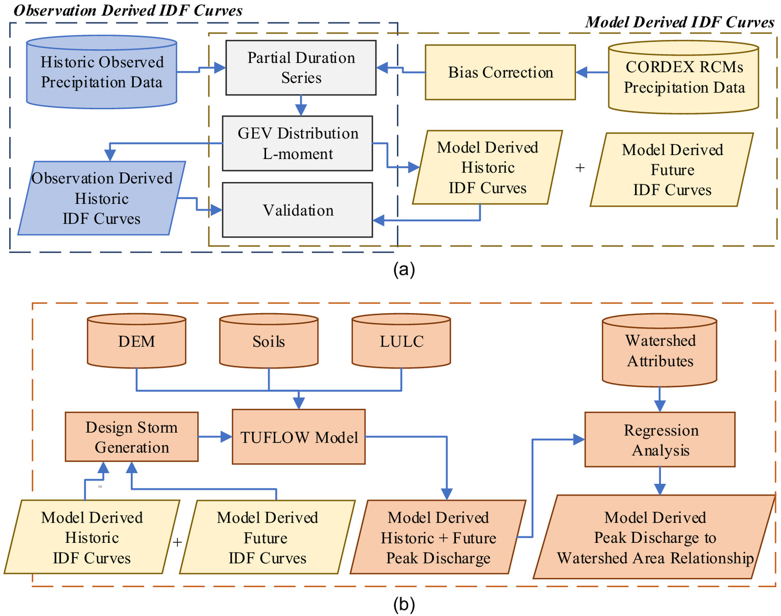
Then, the model-derived IDF curves were created for the same station. This was done by first processing CORDEX RCMs data for a historical period to compare with the Atlas 14 and Smirnov et al. (2018) results, but using modeled data of a historical period instead of historical observed data. Next, the same procedure was repeated for future periods and compared with Smirnov et al. (2018) but not with Altas 14 because Altas 14 is only historical. Model-derived IDF curves were then developed for the other 28 weather stations across Virginia to better understand the spatial variability in future precipitation changes for the region.
The second part of the workflow covers peak discharge estimation using the model-derived IDF curves developed in the first part [Fig. 1(b)]. This part involved, first, numerical modeling by developing a 2D hydrodynamic model using the Two-Dimensional Unsteady Flow (TUFLOW) model for the study watershed located in the coastal plain of Virginia. The model-derived IDF curves were then used to estimate future peak discharge for storms with different return periods and emission scenarios. Finally, regression analysis was used to relate the increase in peak discharge to watershed size for different return periods under different climate scenarios. The following subsections explain each of these steps in further detail.
IDF Curve Development
Observation-Derived IDF Curves
Historical Observed Precipitation Data
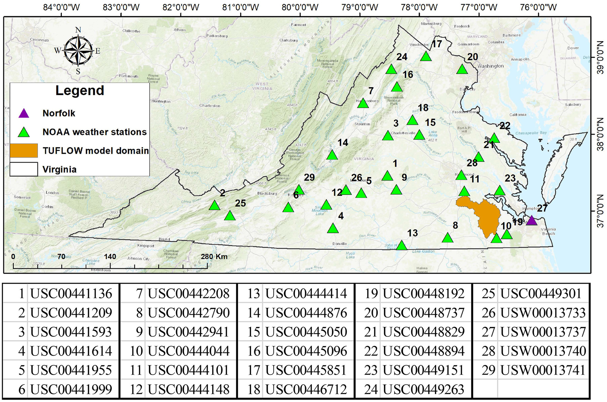
The IDF curves were developed for 29 NOAA weather stations covering Virginia (Fig. 2 and Table S1 ). These stations were selected because they have a precipitation record of a minimum of 50 years without missing data for more than 2 years. The Norfolk International Airport station (USW00013737) was used to develop the methodology for updating IDF curves because it has one of the longest precipitation records (1945 to present) in Virginia (Sadler et al. 2018). Doing so also provides an opportunity to compare our results with a prior study in the region (Smirnov et al. 2018).
The historical daily precipitation data for the 29 selected weather stations were collected from the National Climatic Data Center (NCDC), now the National Centers for Environmental Information (NCEI) (NCEI 2019). Observation-derived IDFs were calculated with 24-h precipitation data for the period 1950 to 2005 for return periods of 1, 2, 5, 10, 25, 50, and 100 years.
Partial Duration Series and Generalized Extreme Value Distribution L-Moment
For the IDF curve development, the Partial Duration Series (PDS) was estimated to be consistent with NOAA Atlas 14 IDF curves (NOAA 2019). The PDS counts every precipitation value above a defined threshold regardless of when it occurred during the period of analysis, whereas the Annual Maximum Series (AMS) uses the highest value per year. The PDS has been shown to provide higher values for return periods shorter than 10 years (Armstrong et al. 2012; Roy et al. 2019). Therefore, PDS is a more conservative approach for the infrastructure design. Smirnov et al. (2018) also developed IDFs using PDS for RCP8.5 and recommended them for future studies. Hence, PDS was used in this study.
Several PDS thresholds were tested to match the generated IDF values to the NOAA Atlas 14 IDF values for the current scenarios at a station. The threshold that minimized the differences between our values and NOAA ATLAS 14 values was selected. Subsequently, the threshold was used to generate the IDF values for future scenarios as well. This analysis was repeated for each of the stations.
Consistent with Atlas 14, the PDS was multiplied by a factor (1.13) to convert daily precipitation to 24-h precipitation as also done in Atlas 14. Work through Atlas 14 found that Generalized Extreme Value (GEV) is the most suitable statistical distribution for the stations of Virginia (Bonnin et al. 2006). Therefore, the PDS was fit to the GEV with L-moments to calculate distribution parameters.
Method Validation
The Norfolk International Airport station was used as the initial case to prepare and validate the code for generating the IDF curves because this is the station used by Smirnov et al. (2018). The calculated observation-derived historical IDF curves for the Norfolk International Airport station were then compared with Atlas 14 and Smirnov et al. (2018). The workflow for producing observation-derived IDFs from historical data using open-source tools and libraries in R and Python is shown in Fig. S1 , and the code is available as described in the “Data Availability Statement.”
Model-Derived IDF Curves
Daily Precipitation from CORDEX RCMs
GCMs from the Coupled Model Intercomparison Project Phase 5 (CMIP5) (ESGF@DOE/LLNL 2019) were used to create future model-derived IDF curves. Because the GCM outputs are spatially coarse, downscaled RCM outputs were obtained from CORDEX (2019). In this study, we used dynamic downscaled models from GCMs provided by CORDEX. Table 1 lists the GCM-RCM information, including spatial and temporal resolution of the five climate models used for the RCP4.5 scenario and the 10 climate models used for the RCP8.5 scenario. Daily RCM precipitation time series were obtained from 1950 to 2100, with 1950–2005 considered as the historical period and 2006–2100 considered as the future period.
| Scenario | Modeling institute | GCM | RCM | Resolution (km) | Frequency |
|---|---|---|---|---|---|
| RCP4.5 | Canadian Centre for Climate Modeling and Analysis | CanESM2 | CanRCM4 | 22 | Daily |
| Canadian Centre for Climate Modeling and Analysis | CanESM2 | CRCM5-UQAM | 44 | Daily | |
| Canadian Centre for Climate Modeling and Analysis | CanESM2 | RCA4 | 44 | Daily | |
| European Centre for Medium-Range Weather Forecasts | EC-EARTH | HIRHAM5 | 44 | Daily | |
| European Centre for Medium-Range Weather Forecasts | EC-EARTH | RCA4 | 44 | Daily | |
| RCP8.5 | Canadian Centre for Climate Modeling and Analysis | CanESM2 | CanRCM4 | 22 | Daily |
| Canadian Centre for Climate Modeling and Analysis | CanESM2 | CRCM5-OUR | 22 | Daily | |
| Canadian Centre for Climate Modeling and Analysis | CanESM2 | CRCM5-UQAM | 22 | Daily | |
| Canadian Centre for Climate Modeling and Analysis | CanESM2 | RCA4 | 44 | Daily | |
| European Centre for Medium-Range Weather Forecasts | EC-EARTH | RCA4 | 44 | Daily | |
| Geophysical Fluid Dynamics Lab | GFDL-ESM2M | CRCM5-OUR | 22 | Daily | |
| Geophysical Fluid Dynamics Lab | GFDL-ESM2M | WRF | 44 | Daily | |
| Max Planck Institute for Meteorology | MPI-ESM-LR | WRF | 22 | Daily | |
| Max Planck Institute for Meteorology | MPI-ESM-LR | RegCM4 | 22 | Daily | |
| Met Office Hadley Centre | HadGEM2-ES | WRF | 22 | Daily |
Precipitation at each station was extracted from the RCM grids using the nearest neighbor method. The modeled precipitation data were collected for two emission scenarios: RCP4.5 and RCP8.5. These are two of the four RCPs with RCP4.5 considered as the intermediate (mitigation) greenhouse gas emission scenario and RCP8.5 considered as the very high greenhouse gas emission scenario, as defined in the Fifth Assessment Report (AR5) of the Intergovernmental Panel on Climate Change (IPCC) (IPCC 2014). The historical NCEI data and downscaled RCM CORDEX data for the 29 stations were processed using Python and R, and this code is available as described in the “Data Availability Statement.”
Bias Correction
The historical precipitation data (1950–2005) from RCMs for both RCP scenarios were compared with historical observations at NOAA weather stations, followed by bias correction. The empirical quantile mapping (EQM)/quantile-quantile () plot was used for bias correction. The EQM corrects the distribution function of climate-simulated values according to the observed distribution function by applying a transfer function (TF). Quantile mapping–based statistical downscaling models assume stationarity, i.e., the relationship between the RCM and the observed data remains the same for the projected period. However, this approach has been successfully used in many studies for developing nonstationary extreme precipitation from RCMs due to its accuracy and simplicity, and it was found to be the most appropriate among different statistical bias-correction methods (Kuo et al. 2015; Teutschbein and Seibert 2012). This method was performed for all climate models mentioned in Table 1 using R’s “downscaleR” package (Iturbide et al. 2019; Bedia et al. 2020). Figs. S2(a and b) show the Q-Q plot for two models Canadian Earth System model (CanESM2_) Canadian regional climate model (CanRCM4), and CanESM2_CRCM5-Université du Québec à Montréal (UQAM), respectively. The modeled data were slightly biased for CanESM2_CanRCM4, whereas the modeled data were highly biased for CanESM2_CRCM5-UQAM.
Partial Duration Series and GEV Distribution L-Moment
As described for the observation-derived IDF curve development, a PDS was also used for the model-derived IDF curve development. However, instead of using historical observed time series records from weather stations, we used the downscaled GCM model output after it was bias corrected using a Q-Q plot procedure, as described in the prior section. We again used the GEV distribution L-moment to generate the historical and future IDF curves.
Model-Derived Historical and Future IDF Curves
To produce updated historical and future IDF curves from RCMs for a given station, the time-series precipitation projections from RCMs within the region of that station were extracted for the period 1950 to 2100. The bias-corrected PDS was fit to the GEV with L-moments, as described previously. After developing the IDF curves from models for the historical scenario (1950–2006), the future IDF curves were calculated for the midcentury (2045) and end-century (2085) periods for both the RCP4.5 and RCP8.5 scenarios. A 30-year time window was used to calculate future precipitation IDF curves, i.e., 2045 represents the period 2030–2060 and 2085 represents the period 2070–2100. The workflow for producing the model-derived historical and future IDF values from RCMs data is shown in Fig. S3 . The code is available as described in the “Data Availability Statement.”
A similar IDF analysis as described previously was performed for the other 28 NOAA weather stations across the state to explore spatial trends across Virginia. Later, the model-derived historical IDF depths were compared with the model-derived future IDF depths to better understand the projected changes in precipitation intensities across Virginia.
Peak Discharge Estimation
Design Storm Generation
The first step in estimating peak discharge was the generation of design storms for different return periods under different climate scenarios. For this purpose, the 24-h design storm hyetographs for seven different return periods (1, 2, 5, 10, 25, 50, and 100 years) were generated using a NOAA Type B unit hyetograph for both the model-derived historical and future periods under both the RCP4.5 and RCP8.5 scenarios. The 24-h rainfall duration is often used in the design of the hydraulics structures (VDOT 2021). Moreover, it was used by Smirnov et al. (2018), which was used to validate our software. These design storm inputs were later used in a 2D hydrodynamic model to estimate the peak discharge resulting under the different climate scenarios for the midcentury (2045) and end-of-century (2085) periods.
TUFLOW Model
For estimating peak discharge, a 2D hydrodynamic model was developed for a basin in the coastal plain of Virginia. The TUFLOW model was used due to its ability to solve the shallow water equations (SWE) over complex terrains, making it valuable given the flat topography of the coastal plain. The model domain is located in the southeastern part of Virginia (Fig. 3) and is designated as 03010202 in the hydrologic unit maps (DCR 2021). It consists of portions of Prince George, Sussex, Slurry, Southampton, and Isle of Wright counties, covering a total area of approximately (665 sq mi).
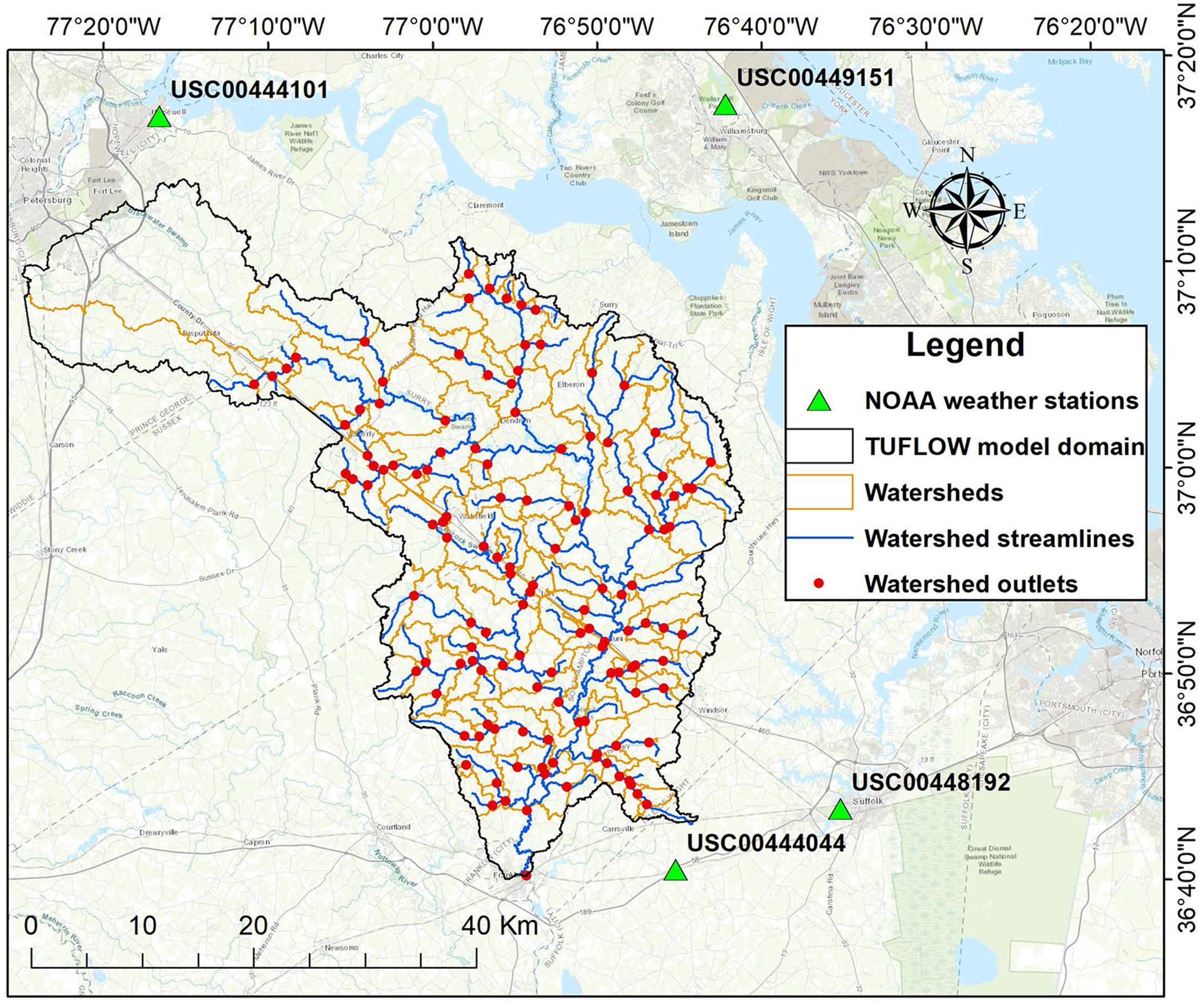
Four surrounding NOAA weather stations [USC00444101 (Hopewell), USC00444044 (Holland 1 E), USC00448192 (Suffolk Lake Kilby), and USC00449151 (Williamsburg 2 N)] were used to create the precipitation inputs for the TUFLOW model using a 24-h design storm generated with the methods described previously. The spatial interpolation of precipitation was done using the inverse distance weighted (IDW) method with an exponent value of 2 (integrated within the TUFLOW model) to uniformly distribute the storms over the study area.
The TUFLOW model used in this study region was previously developed and calibrated by Morsy et al. (2018, 2021). A summary table of the parameters considered for the TUFLOW model development is given in Table 2. The model bathymetry was primarily developed with a 10-m digital elevation model (DEM), including a 1-m DEM for low-relief terrain, where available. The river bathymetry at bridge cross sections was obtained through site visits. The mesh size of the model was 30 m. The roughness coefficient (i.e., Manning’s ) was the calibration parameter. Different Manning’s values were assigned to different surface materials. The outlet of the watershed was located at a USGS station that measured stage depth. The model was calibrated against observed stage depth (i.e., water level) at nine USGS stations for Hurricane Matthew. The average relative error (RE) and Nash-Sutcliffe efficiency (NSE) were found to be 5.15% and 0.67, respectively. The TUFLOW model domain included 131 georeferenced Virginia Department of Transportation (VDOT) bridges and culverts, shown as watershed outlets in Fig. 3. The regression analysis was applied to all 131 of these watersheds that have varying sizes to investigate the relationship between the future peak discharge and watershed size.
| Parameters | Description | USGS stage Observation Station ID |
|---|---|---|
| Mesh size/cell resolution | 30-m Cartesian grid resolution | — |
| DEM | 10- and 1-m DEM (where available) | — |
| River bathymetric data | Conducted site visit surveys | — |
| LULC | 30-m LULC with 3-m resolution near channels and in floodplain | — |
| Soil | County-scale soil data from SSURGO (2018) | — |
| Manning’s | Deciduous , evergreen , mixed , , , , , and emergent herbaceous | — |
| Model calibration | Hurricane Matthew (October 10–24, 2016) | 02045500, 02047000, 02052000, 02052090, 02047500, 02047783, 02049500, 02050000, 02047370 |
| Model evaluation | Unnamed storm (October 10–24, 2018) |
Note: LULC = land use and land cover.
Model-Derived Future Peak Discharge
Historical discharges were obtained by simulating the TUFLOW model using the historical model-derived IDF curves from the RCMs analysis under both the RCP4.5 and RCP8.5 scenarios. Next, the future scenarios were simulated by TUFLOW using model-derived future IDF curves for the two emission scenarios, each with two time spans centered on 2045 and 2085. A total of 28 increase results (seven return periods under two emission scenarios and on 2 target years) were obtained (Table S2 ), comparing the of the future simulation with that of the historical. For each watershed outlet, the computed percent increase was calculated as follows:where and = future and historical peak discharge, respectively.
(1)
Regression Analysis
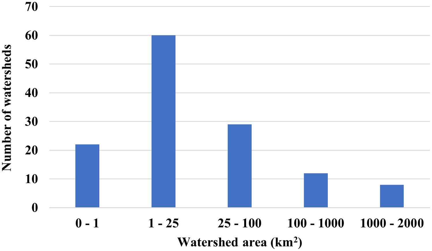
A regression analysis was conducted to investigate the relationship between peak discharge and watershed area. The size of the watersheds ranged from 0.003 (0.001) to (655 sq mi). The distribution of the watershed areas is shown in Fig. 4.
Results
IDF Curve Development
Validation of IDF Curve at Norfolk, Virginia
The open-source libraries and tools used in this study need validation before being used across the gauging stations. This validation was done at the Norfolk International Airport station, as mentioned previously. The observation-derived IDF curves for the Norfolk International Airport station for the historical periods were replicated from the historical data and compared with both Atlas 14 and Smirnov et al. (2018). The result of this comparison confirmed that the tool produces very similar IDF curves as those available in NOAA Atlas 14 and from Smirnov et al. (2018).
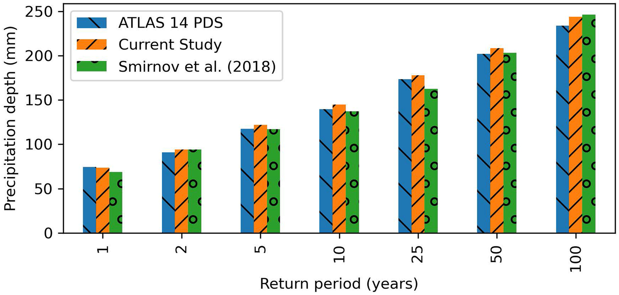
Fig. 5 shows the model-derived historical IDF depths from the current study compared with those from Atlas 14 and Smirnov et al. (2018). The bar chart shows that the model-derived historical IDF depths were very similar to the Atlas 14 values. The largest difference in the model-derived IDF depths between this study and Atlas 14 was for the 100-year storm, which was 4% higher than the Atlas 14. The model-derived IDF depths generated in this analysis were similar to those reported by Smirnov et al. (2018).
The methods were next used to estimate the model-derived IDF curves for future periods using the projected climate data from the RCMs at the same station. Table 3 presents the IDF depths using the RCM data for periods 2045 and 2085 and the percent increases compared with the historical periods under the RCP4.5 scenario. It is important to note that the model-derived historical IDF depths for the current study were not the same as those in Fig. 5 because the RCMs used in the RCP4.5 were different from those used in the RCP8.5.
| Return period (years) | Historical period | 2045 | 2085 | |||
|---|---|---|---|---|---|---|
| Atlas 14 PDS | Current study (mm) | Current study (mm) | Increase (%) | Current study (mm) | Increase (%) | |
| 1 | 73.7 | 71.1 | 71.1 | 0 | 78.7 | 11 |
| 2 | 91.4 | 91.4 | 88.9 | 99.1 | 8 | |
| 5 | 116.8 | 116.8 | 114.3 | 127.0 | 9 | |
| 10 | 139.7 | 134.6 | 137.2 | 2 | 152.4 | 13 |
| 25 | 172.7 | 167.6 | 172.7 | 3 | 190.5 | 14 |
| 50 | 203.2 | 193.0 | 205.7 | 7 | 228.6 | 18 |
| 100 | 233.7 | 226.1 | 246.4 | 9 | 271.8 | 20 |
Table 3 indicates that the percent increase in the model-derived IDF depth under the RCP4.5 scenario was less than 10% in the 2045 period. Generally, the percent increase was smaller with smaller design storms and even decreased or remained the same for the 5-, 2-, and 1-year return periods. In the year 2085, however, the percent increase was significantly larger, ranging from 8% to 20%, and was again generally smaller for lower-return-period design storms. Comparison with Smirnov et al. (2018) was not possible for these specific results because Smirnov et al. (2018) developed the model-derived IDF curves for the RCP4.5 scenario based on AMS instead of PDS.
Table 4 presents the model-derived future IDF depths for periods centered on 2045, 2075, and 2085 and the percent increase compared with the historical periods and Smirnov et al. (2018) under the RCP8.5 scenario. The model-derived historical IDF values for RCP4.5 and RCP8.5 are different in Tables 3 and 4 because they were created using different RCMs and spatial resolutions. The model-derived future IDF curves for the 2075 period using RCP8.5 were included to compare with the available IDF curves of Smirnov et al. (2018) for the same year.
| Return period (years) | Historical period | 2045 | 2075 | 2085 | |||||||||
|---|---|---|---|---|---|---|---|---|---|---|---|---|---|
| Atlas 14 PDS (mm) | Current study (mm) | Smirnov et al. (2018) (mm) | Current study (mm) | Increase (%) | Smirnov et al. (2018) (mm) | Increase (%) | Current study (mm) | Increase (%) | Smirnov et al. (2018) (mm) | Increase (%) | Current study (mm) | Increase (%) | |
| 1 | 73.7 | 73.7 | 68.6 | 78.7 | 7 | 76.2 | 11 | 83.8 | 14 | 81.3 | 19 | 83.8 | 14 |
| 2 | 91.4 | 94.0 | 94.0 | 109.2 | 16 | 111.8 | 19 | 116.8 | 24 | 116.8 | 24 | 119.4 | 27 |
| 5 | 116.8 | 121.9 | 116.8 | 147.3 | 21 | 139.7 | 20 | 157.5 | 29 | 149.9 | 28 | 162.6 | 33 |
| 10 | 139.7 | 144.8 | 137.2 | 177.8 | 23 | 165.1 | 20 | 188.0 | 30 | 180.3 | 31 | 193.0 | 33 |
| 25 | 172.7 | 177.8 | 162.6 | 223.5 | 26 | 198.1 | 22 | 238.8 | 34 | 215.9 | 33 | 241.3 | 36 |
| 50 | 203.2 | 208.3 | 203.2 | 264.2 | 27 | 251.5 | 24 | 284.5 | 37 | 276.9 | 36 | 284.5 | 37 |
| 100 | 233.7 | 243.8 | 246.4 | 312.4 | 28 | 302.3 | 23 | 335.3 | 38 | 335.3 | 36 | 335.3 | 38 |
The increases were much higher for the RCP8.5 than for the RCP4.5 scenario, as expected. In the 2045 period, the five largest of the seven design storms had increases of between 20% and 30%. In the 2085 period, these increases were all between 30% and 40%. When comparing the periods 2075 and 2085, the values did not increase for the highest (100-year) and lowest (1-year) storms; however, there was a slight increase for the other return periods. In general, the IDF depths estimated in this study were comparable to Smirnov et al. (2018) as well. The estimates for the 2075 period were nearly identical. For example, the 100-year event had 2% higher precipitation compared with Smirnov et al. (2018). However, the estimates for the 2045 period showed larger differences. The larger return period storms especially had larger increases in this study compared with Smirnov et al. (2018). For example, the 100-year event had a 5% higher precipitation increase compared with Smirnov et al. (2018).
Results in Table 4 further suggest that the recommendation made by Smirnov et al. (2018) to increase precipitation intensity by 20% is appropriate and may even underestimate the climate change impact on IDFs for higher return periods. The estimates from the current study for the higher return period storms centered around 2045 were closer to 30% in this study. Additionally, for infrastructure with a longer design life (e.g., 50 years), the results suggested a larger percent increase of more than 30% could be more appropriate for design storms larger than the 2-year event centered on 2075. The difference between these results may be explained by differences in the exact RCMs used in the two studies and the application of slightly different methods and tools.
The results also show how future emissions will impact future design storms. For example, the differences between the model-derived IDF estimates under the RCP8.5 scenario were nearly double those under the RCP4.5 scenario. This impact of different scenarios was much larger than the impact of the time frame. In fact, the estimates centered on 2045 for the RCP8.5 scenario were greater than those centered on 2085 for the RCP4.5 scenario.
Model-Derived Future IDF Curves across Virginia
The model-derived IDF curves were developed at 29 NOAA weather stations across Virginia for 28 combinations, as summarized in Table S2 . We found an increase in the precipitation intensity in almost all stations, but the amount of increase was variable across the stations. The spatial variation of precipitation increases across the state, both in magnitude and percentage, is shown in Fig. 6, along with the five geologic regions (Coastal, Piedmont, Blue Ridge, Valley and Ridge, and Appalachian) of Virginia as background. The percent increase provides additional information that better represents the degree to which the increases in precipitation vary across the state. These results were based on the median of RCM outputs for the 100-year event in the 2085 period using the RCP4.5 [Figs. 6(a and b)] and RCP8.5 [Figs. 6(c and d)] scenarios.
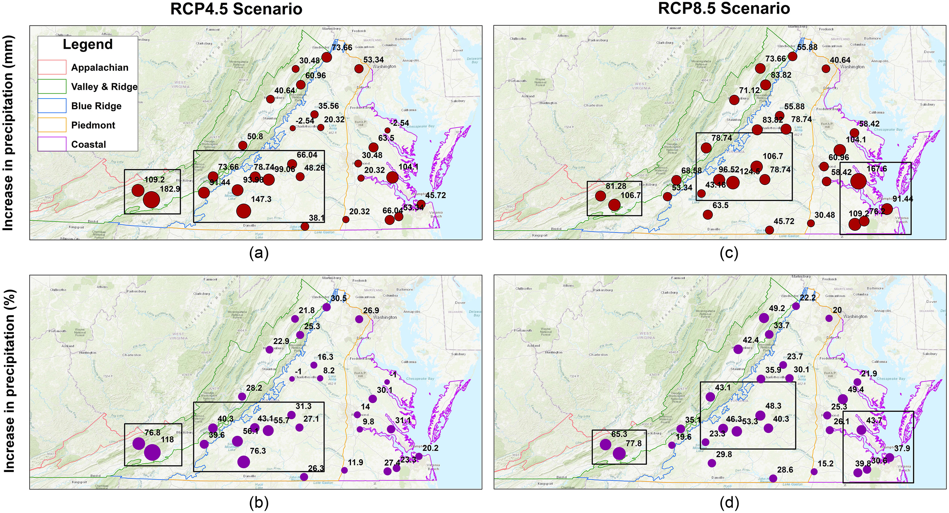
For RCP4.5, the change in IDF depths ranged between and 182.9 mm, and the percent change ranged between and 118 % [Figs. 6(a and b)]. An increase was found in all the stations except two: Charlottesville and Warsaw. The negative percent increase at the end of the century (2085) might reflect the mitigation scenario of RCP4.5. The southern piedmont and southern mountainous (Blue Ridge and Valley and Ridge) regions had stations with the largest absolute increase and percent increase (highlighted with a box). The largest increase was in the Wytheville and Tazewell, with 182.9 mm (118%) and 109.2 mm (77%), respectively, near New River in Blacksburg.
For RCP8.5, the change in IDF depths ranged from 30.5 to 167.6 mm [Fig. 6(c)], and the percent change ranged from 15.2% to 77.8% [Fig. 6(d)]. The southern side of the coastal plain, piedmont, and mountainous (Blue Ridge and Valley and Ridge) regions had stations with larger increases (highlighted with a box), with no obvious spatial pattern. The largest increase was 167.6 mm and was located in the Middle Peninsula of the Hampton Roads region. However, the station closest to it had an increase of only 58.42 mm. Similarly, in the Piedmont region, stations near Lynchburg had increases of 96.5 and 124.5 mm, whereas a nearby station only had an increase of 43.2 mm. The percent increase better informs the extent to which the rain has increased from its historical values.
For example, although the precipitation increase at the two most southwesterly stations (81.3 and 106.7 mm) was much smaller than that of the Hampton Roads region (167.6 mm), these two southwest stations had the largest percent increase (65.3% and 77.8%). Therefore, even though the absolute increase in precipitation was similar to many other stations in the state, the increase may be felt more substantially in these two stations where there has historically been less rainfall.
Overall, although there was substantial variability in the projected increases of precipitation across individual stations, there was no clear spatial trend in the variation of increases across the state for RCP4.5 and RCP8.5 scenarios. However, the southern part of Virginia seemed more prone to increased precipitation in both scenarios. Among the largest cities, Richmond will experience an increase of 30.5 mm (14%) and 61 mm (25.3%) by the end of this century under RCP4.5 and RCP8.5, respectively, for a 100-year storm event. Norfolk, which is also flood vulnerable, showed an increase of 45.7 mm (20.2%) and 91.4 mm (37.9%) for a 100-year storm event under RCP4.5 and RCP8.5, respectively, by the end of this century.
The comparison between RCP4.5 and RCP8.5 further indicated that, in general, the mitigation scenario RCP4.5 has lower precipitation increases than the high-emission scenario RCP8.5. However, this pattern differed for eight stations, where the precipitation (mm) is higher in RCP4.5, and for nine stations, where the precipitation (%) is higher in RCP4.5. These stations are clustered into two groups, as depicted in Figs. S4(a and b) . One of the clusters includes the stations in the southwest of Virginia. Another cluster covers two stations in northern Virginia: Washington and Winchester.
The climate models used for RCP4.5 and RCP8.5 were of different RCMs and spatial resolutions (Table 2). Hence, the two scenarios’ historical values also differed (Tables 3 and 4). This might be one of the reasons behind this unexpected difference in the comparison. If we had the same models with similar resolution for both scenarios, we might be better able to compare the RCP scenarios. Because the clusters’ stations are in close proximity, it was assumed that the anomalies came from the uncertainty associated with the climate models, which ultimately translated into future precipitation magnitudes and caused inconsistent values at some stations in the study area.
The statistical distribution of increases in precipitation across the 29 observation stations for the seven return periods analyzed are shown in Fig. 7. This boxplot indicates that the median increase in precipitation depth was well above 20% among all stations by midcentury in the RCP8.5 scenario. This reinforced the results found for the Norfolk International Airport station. The median increase for most design storms was close to or above 40% by the end of the century. Fig. 7 also highlights the variation across the stations for the different scenarios. Overall, the median increase of projected precipitation in Virginia was between 10% and 30% for midcentury and 10% and 40% for the end of the century for the RCP4.5 and RCP8.5 scenarios, respectively.
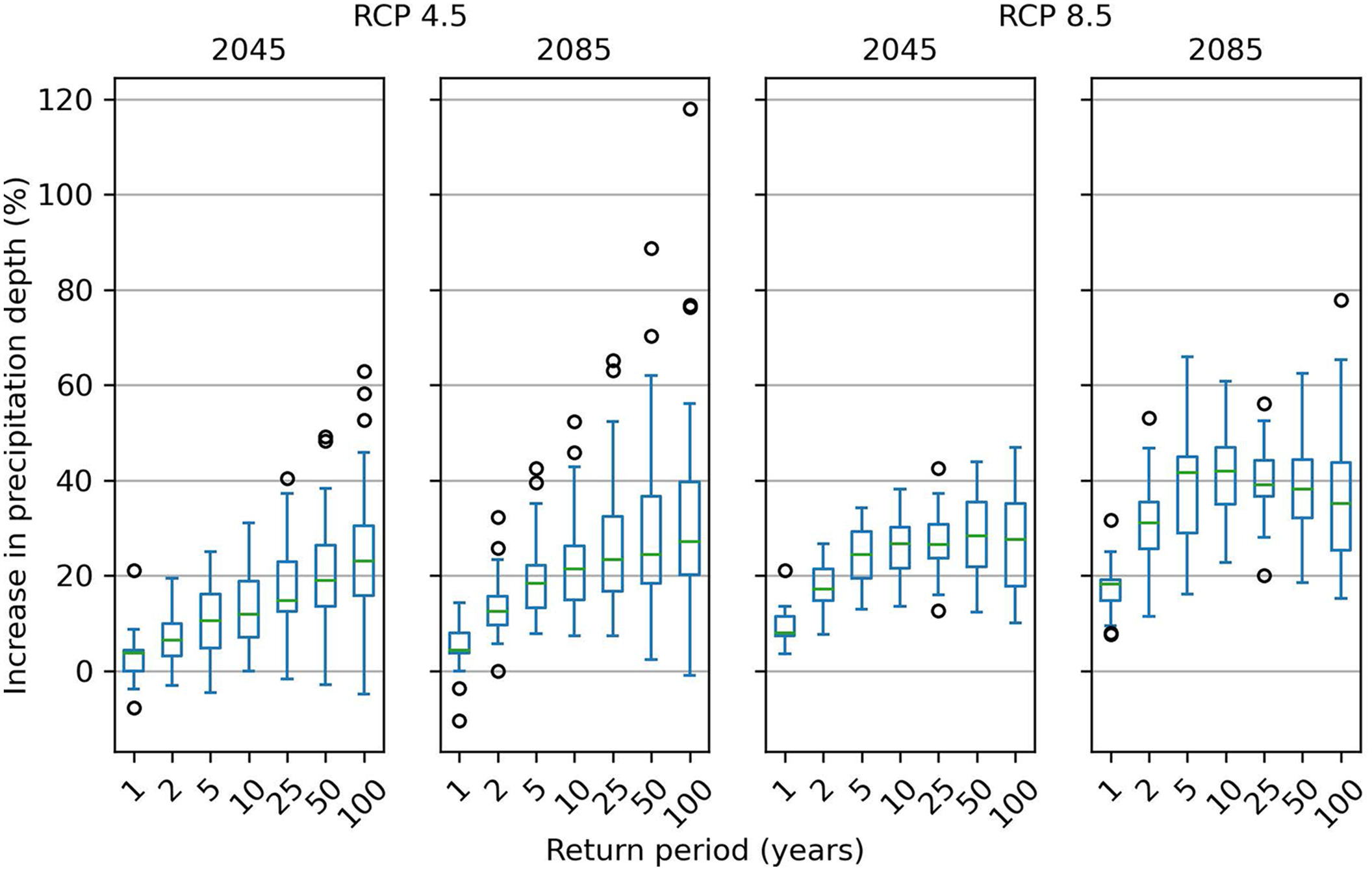
The boxplots further reveal that the median of the percent increase for the RCP8.5 scenario was greater than those of the RCP4.5 scenario, as expected (IPCC 2014). However, the variability in the RCP4.5 scenario was much greater than in the RCP8.5 scenario. There was far more range in the RCP4.5, and many values were on the upper end of the distribution. Hence, the increases of RCP4.5 were greater than those of RCP8.5 in the higher return period storms. This may be an artifact of the differences in models available for use in the RCP4.5 scenario versus in the RCP8.5 scenario. To the best of our knowledge, these were all the high-resolution RCMs available at the time this study was completed. However, these issues can be further investigated in the future using the same RCMs models of the same resolution.
Peak Discharge Estimation
Model-Derived Future Peak Discharge
The design storms developed from model-derived IDF curves were translated to peak discharge using the TUFLOW hydrodynamic model at 131 bridge locations with varying watershed sizes, and the percent increase was calculated for each location. There was a percent increase in peak discharge in all locations for all return periods under both emission scenarios. The response of peak discharge for different watershed sizes was divided into two categories: the watersheds with an area were categorized as smaller” watersheds, whereas those with an area were categorized as larger watersheds. The percent increase of peak discharge from the 100-year storm event for the 2045 and 2085 periods under RCP4.5 and RCP8.5 are shown in Fig. 8 for all watersheds (trendline was fit for all watersheds with area ), and only smaller watersheds (trendline was fit for all watersheds with area ).
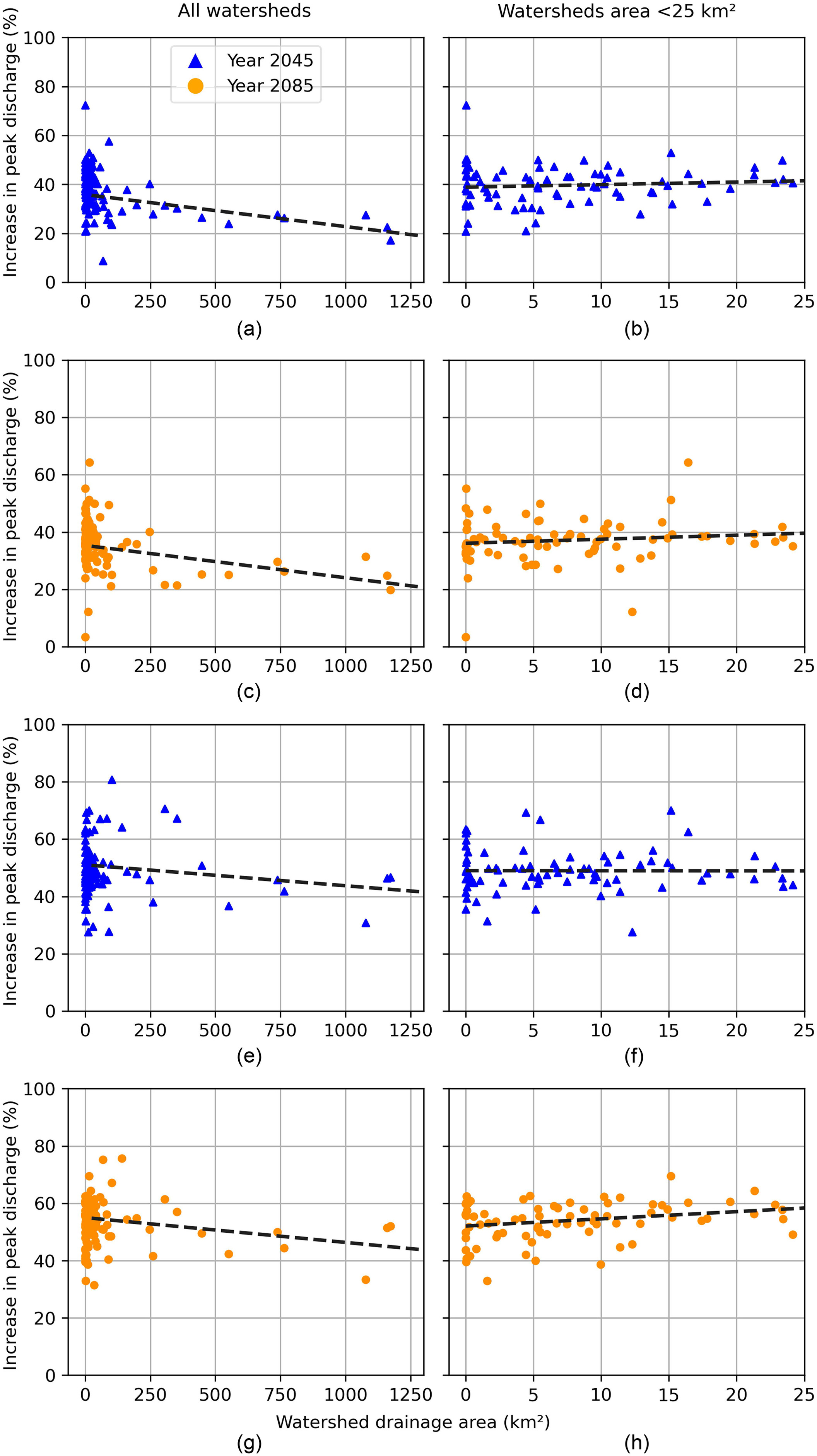
The figure shows that the change in peak discharge was more scattered in the watersheds with smaller drainage areas. When looking only at the smaller watersheds (area ), no clear trend with drainage areas was found [Figs. 8(a, c, e, and g)]. Overall, however, larger watersheds (area ) had a smaller percent increase [Figs. 8(b, d, f, and h)]. One possible reason is that the runoff has more space (longer reach lengths, wider floodplains, and larger storage) and time (longer time of concentration, lag time, and response time) in larger watersheds. In general, this would allow the water to spread out more across the watershed, reducing the percent increase of peak discharge, although it might not reduce the total runoff volumes of the watershed.
Model-Derived Future Peak Discharge to Watershed Area Relationship
Fig. 9 shows the percent increase in peak discharge for 1-, 10-, and 100-year design storms against the watershed area for the 2045 and 2085 periods under the RCP4.5 scenario. The same plot, but for all seven design storms, is given in Fig. S5 . These plots show a linear trend line that fits the points with drainage areas greater than . In the 1-year event, the trend line was essentially flat with a higher magnitude slope in the discharge response to the 100-year event.
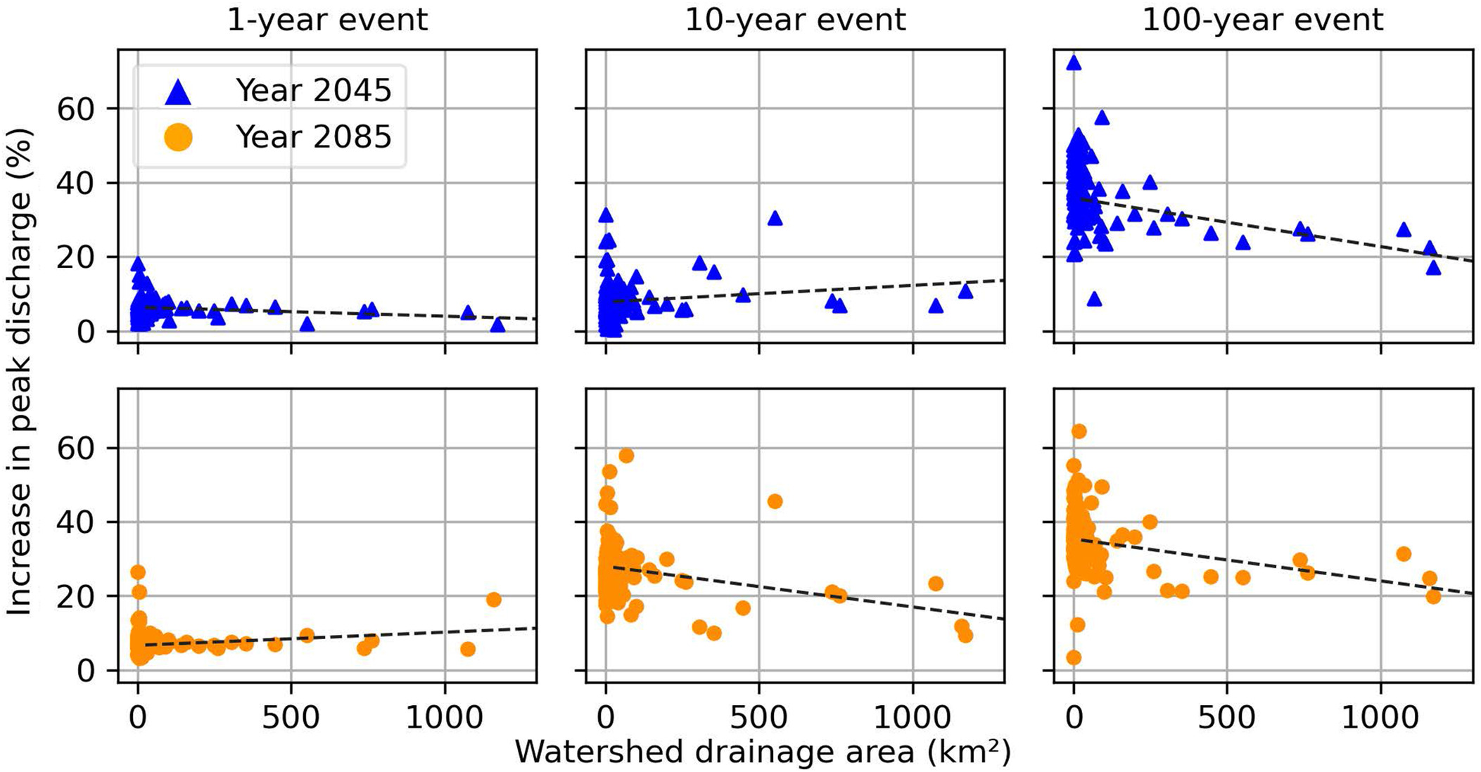
The regression equations for the trend lines of percent increase in peak discharge versus watershed area across the different returns periods for RCP4.5 are given in Table 5. Watersheds with a drainage area of less than had a constant percent increase in peak discharge for a given return period, regardless of watershed size. For smaller watersheds, the percent increase in peak discharge across the different return periods was between 5% and 39% in the midcentury and between 8% and 36% at the end of the century under RCP4.5, depending on watershed size.
| Time period | Return period (years) | Increase in peak discharge (%) | Difference between smaller watersheds and largest watershed (%) | ||||
|---|---|---|---|---|---|---|---|
| Watershed area | Watershed area | ||||||
| Regression equation | Correlation coefficient, | Watershed | Watershed | ||||
| 2045 | 1 | 7 | 6 | 2 | 5 | ||
| 2 | 5 | 0.31 | 3 | 6 | |||
| 5 | 6 | 0.01 | 5 | 5 | 1 | ||
| 10 | 9 | 0.26 | 8 | 15 | |||
| 25 | 17 | 16 | 10 | 7 | |||
| 50 | 28 | 25 | 4 | 24 | |||
| 100 | 39 | 34 | 14 | 25 | |||
| 2085 | 1 | 8 | 0.46 | 7 | 13 | ||
| 2 | 18 | 18 | 14 | 4 | |||
| 5 | 31 | 33 | 17 | 14 | |||
| 10 | 27 | 27 | 9 | 18 | |||
| 25 | 35 | 33 | 15 | 20 | |||
| 50 | 36 | 35 | 14 | 22 | |||
| 100 | 36 | 34 | 16 | 20 | |||
For comparison within larger watersheds, we computed the percent increase for two watersheds with a size of (a random watershed with an area ) and (approximately the largest watershed considered in this study). For a 100-year event, the percent increase for the 100- and watersheds was 34% and 14%, respectively, at the midcentury. By the end of the century, the percent increase was still 34% for the watershed and 16% for the watershed. So, the larger watershed had a smaller percent increase than the smaller ones, and the percent increase decreased as the watershed area increased. Across different return periods, the percent increase in peak discharge was found between 2% and 15% in the midcentury and between 9% and 17% at the end of the century for the watershed. The equations across different return periods further show that the slopes for all but four of the 14 equations were negative. Additionally, the magnitude of the negative slopes generally increased with larger storm events, indicating that the percent increase decreased with larger storm events in larger watersheds. This suggests that the smaller watersheds will be affected more significantly than larger ones for larger storm events under the RCP4.5 scenario.
The response of peak discharge for midcentury (2045) and end of the century (2085) of RCP4.5 was also further explored. The largest percent increase between the two time periods, 2045 and 2085, occurred in the midrange of the design storms for RCP4.5 (Fig. 9). When comparing the increase in peak discharge between the 2045 and 2085 periods, there was only a small change in the 1-year event and the 100-year event compared with the 10-year event, where there was a greater percent increase from the 2045 to 2085 periods for many of the watersheds. This suggests that climate change may most impact midrange storms in this region under the RCP4.5 scenario.
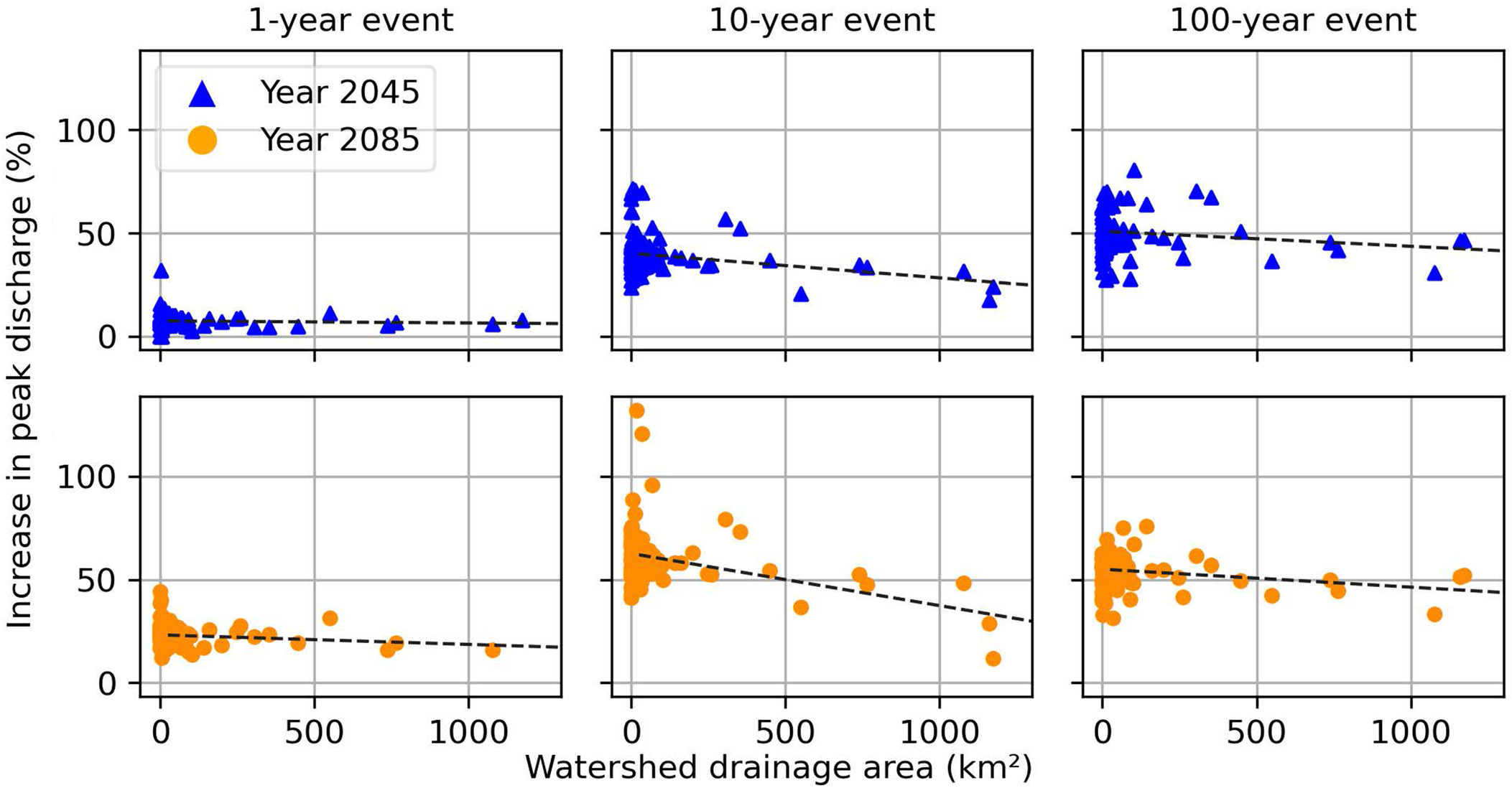
A similar analysis was conducted for the RCP8.5 scenario. Fig. 10 shows the percent increase in peak discharge for the 1-, 10-, and 100-year events over the watershed areas for RCP8.5. Here, it should be noted the range of the -axis in Fig. 10 was considerably larger than that of Fig. 9. Table 6 presents the equations corresponding to the linear trend lines for different return periods.
| Time period | Return period (years) | Increase in peak discharge (%) | Difference between smaller watersheds and largest watershed (%) | ||||
|---|---|---|---|---|---|---|---|
| Watershed area | Watershed area | ||||||
| Regression equation | Correlation coefficient, | Watershed | Watershed | ||||
| 2045 | 1 | 8 | 8 | 6 | 2 | ||
| 2 | 21 | 0.03 | 21 | 22 | |||
| 5 | 32 | 33 | 20 | 12 | |||
| 10 | 41 | 39 | 20 | 21 | |||
| 25 | 46 | 46 | 15 | 31 | |||
| 50 | 48 | 50 | 17 | 31 | |||
| 100 | 49 | 50 | 39 | 10 | |||
| 2085 | 1 | 25 | 23 | 15 | 10 | ||
| 2 | 47 | 46 | 25 | 22 | |||
| 5 | 54 | 56 | 27 | 27 | |||
| 10 | 58 | 60 | 20 | 38 | |||
| 25 | 62 | 61 | 18 | 44 | |||
| 50 | 57 | 63 | 17 | 40 | |||
| 100 | 52 | 54 | 40 | 12 | |||
Keeping consistent with RCP4.5, RCP8.5 also suggested that smaller watersheds will be more sensitive to increased precipitation than larger ones. The percent increases in the RCP8.5 were much greater than the RCP4.5, reaching past 100% for some watersheds and design storms (Fig. S6 ). For the smaller watersheds, the average percent increase in peak discharge was 52% in RCP8.5 (Table 6) compared with 36% in RCP4.5 (Table 5) for the 100-year storm event. Overall, the percent increase in peak discharge was found to be between 8% and 49% in the 2045 period and between 25% and 62% in the 2085 period across different return periods under RCP8.5.
For larger watersheds, the percent increase for a 100- and watershed was 50% and 39%, respectively, for a 100-year storm event in the midcentury. The percent increase was 54% and 40%, respectively in the 2085 period. Like RCP4.5, RCP8.5 also resulted in a smaller percent increase in peak discharge for larger watersheds compared with smaller ones, and the percent increase decreased as the watershed area increased. Across different return periods, the percent increase range for the watershed was between 6% and 39% for the 2045 period and between 15% and 40% for the 2085 period, depending on the return periods.
In summary, considering both RCP4.5 and RCP8.5 scenarios, for the smaller watersheds, the percent increase was 7% and 8% for the 1-year, 9% and 41% for the 10-year, and 39% and 49% for the 100-year return periods of the 2045 time period. For the same return periods, the percent increase was 8% and 25%, 27% and 58%, and 36% and 52%, respectively, for the 2085 time period. For the largest watershed of , the percent increase in peak discharge was 2% and 6% for the 1-year, 15% and 20% for the 10-year, and 14% and 39% for the 100-year return periods for the 2045 time period. For the same return periods, the percent increase was 13% and 15%, 9% and 20%, and 16% and 40%, respectively, for the 2085 time period.
For larger watersheds, the magnitude of the slope of the trend lines was also greater in the RCP8.5 scenario compared with RCP4.5. This indicates that the difference in impact between smaller watersheds and larger watersheds will be more pronounced in the RCP8.5 scenario. The differences in percent increase in peak discharge between small watersheds () and larger watersheds were much higher for RCP8.5 (Table 6) compared with RCP4.5 (Table 5). For example, the maximum difference for the 2045 and 2085 periods was 25% and 22%, respectively, under RCP4.5, whereas it was 31% and 44% for the 2045 and 2085 periods, respectively, under RCP8.5. This suggests that the difference between smaller and larger watersheds will be more significant under the RCP8.5 scenario.
Overall, the regression equations of percent increase in peak discharge for different return periods are easily interpretable and provide the transportation or water resources engineers of VDOT an initial idea about the percent increase in design peak discharge based on the watershed area without creating a complicated, time-consuming hydrologic or hydrodynamic model. Later, further in-depth assessment or hydraulic model simulations can be conducted for the watersheds that are found to be highly sensitive to peak increase.
Discussion
Comparison with Relevant Studies
By the end of this century (2020–2099), Cook et al. (2020) noticed a percent increase in between 5% and 15% (approximately 15%), 15% and 25% (approximately 20%), and 25% and 60% (approximately 30%) for 24-h 25-year storm events in Baltimore, Maryland; Charlotte, North Carolina; and Pittsburg, Pennsylvania, with respect to a baseline of 1953–2013 and for the RCP8.5 scenario. Butcher et al. (2021) also found a significant increase in the 24-h 10-year (15%) and 100-year (10%) return period storms in the future (2050–2080) relative to the baseline (1950–2005) in Durham, North Carolina. In our study, we found that median projected precipitation in Virginia is expected to increase between 10% and 30% by midcentury (2045) and between 10% and 40% by the end of the century (2085) from the baseline (1950–2005). These findings were for both RCP4.5 and RCP8.5 scenarios and across various return periods of 24 h. So, the nearby states also experienced an increasing rainfall depth like Virginia, implying that the current study findings qualitatively matched the existing studies conducted in the region.
We found an increase in peak discharge for all watersheds, but for smaller watersheds, the percent increase in peak discharge was independent of the watershed size, whereas for larger watersheds, the percent increase in peak discharge decreased as the size of the watershed increased. Relevant studies, including those by Ganguli and Coulibaly (2017), Ivancic and Shaw (2015), and Do et al. (2017), among others, reinforced the finding of the current study that larger watersheds had a decrease in the percentage increase of peak streamflow. None of these studies translated model-derived future IDF curves to peak discharge to investigate the relationship of peak discharge with watershed size in detail as we did; instead, they used observed or modeled precipitation to understand the trend of streamflow with respect to the watershed parameters. Still, these studies support the finding of the current study that the percentage increases in peak discharge would be more significant in the smaller watersheds compared with the larger watersheds in the future emission scenarios.
According to Ganguli and Coulibaly (2017), smaller watersheds might have increased flood peaks. On the contrary, the larger watersheds might experience decreased runoff due to lower soil moisture. Ivancic and Shaw (2015) found a similar result for the contiguous US, revealing that the probability of very heavy precipitation events resulting in very high discharge [denoted as was significantly lower in larger watersheds than in smaller ones. The study mentioned that larger basins were more likely to have natural features/storages (e.g., wetlands, valley bottoms, and so on) that attenuated runoff in the watersheds, and consequently reduced the peak discharge in the stream. That study further mentioned that the large basins were more likely to have a long lag time than small ones. So, the longer lag time can result in lower peak discharge in larger watersheds compared with smaller ones.
The annual maximum observed streamflow trends were analyzed by Do et al. (2017) on a global scale, concluding that the smaller watersheds experienced increasing streamflow trends whereas the larger ones experienced decreasing trends. They explained that larger watersheds generally experienced long-duration rainfall events; thus, the climatic forcings might act differently on these larger watersheds compared with smaller ones.
Study Limitations and Opportunities for Future Research
One of the limitations of this study is the uncertainties inherited from different numerical models. In this study, the IDF curves were derived from an ensemble of RCMs. Later, these IDF curves were also used as input for the 2D hydrodynamic model. Each RCM has its parameterizations and simplification methods that introduce uncertainty in the outputs. Although the ability of the RCMs to model future conditions with accuracy is uncertain, the models were bias-corrected and have been shown to replicate historical climatic patterns adequately, lending confidence in their use. Moreover, several RCMs (five RCMs for RCP4.5 and 10 RCMs for RCP8.5) were used as an ensemble to capture uncertainty across the RCMs.
Furthermore, the TUFLOW model was used for calculating discharge over the study area. As with the RCMs, the TUFLOW model has also been calibrated and demonstrated to adequately represent the physical behavior of the discharge (Morsy et al. 2018, 2021). However, similar to RCMs, the accuracy of the TUFLOW model in representing the behavior of discharge in such a large basin is uncertain, and thereby, the results must be interpreted prudently with proper judgment. Additionally, the regression equations are based on a model of only one geographic region in Virginia. Generalizing the regression equations between discharge and watershed area from one region to another would require further analysis and exploration of the watershed geomorphology, retardation, diffusive effects, and so on (Huang and Willgoose 1993). Therefore, these should be investigated case by case, as suggested by DeGaetano and Castellano (2017), because watersheds with different physical characteristics may respond differently to increases in design storm volumes. In the future, similar regression equations can be developed over other watersheds of Virginia as well to better understand the regional variability in the impact of future climate change on peak discharge for watersheds if varying sizes.
Another potential opportunity for future research is to compare the model-derived IDF curves with the next-generation precipitation frequency standard, NOAA Atlas 15, currently in progress (Kim et al. 2023; NOAA 2023). NOAA Atlas 15 will account for temporal trends in historical observations and use future climate model projections to generate adjustment factors. It will be developed based on historical data and nonstationarity assumptions using the latest precipitation observations and future climate model projections. Although the incorporation of the snowmelt-driven flood is still under consideration, it is expected that regional climate characteristics, such as cold or warm climates and snow-dominated or rain-dominated areas, would be considered (Kim et al. 2023). With the current timeline, the Atlas 15 is expected to be available for contiguous United States (CONUS) by 2026 and outside of CONUS by 2027 (NOAA 2023).
Conclusion
The observation-derived IDF curves developed by the NOAA Atlas 14 using historical precipitation are still the primary data source for civil infrastructure design. Considering the observed and climate model projected intensification of extreme precipitation, the design guidelines should ideally incorporate nonstationary climate conditions. This study outlined an approach for estimating model-derived IDF curves from RCM outputs under nonstationary conditions using open-source software packages that are relatively simple and easily reproducible for any station with long-term historical precipitation records. This approach was based on the statistical EQM bias correction and GEV distribution methods, consistent with NOAA Atlas 14, and it provided reliable/trustworthy historical results when compared with Atlas 14 and Smirnov et al. (2018).
The model-derived IDF framework was applied at 29 stations across Virginia to estimate IDF curves for midcentury and end-of-the-century periods under RCP4.5 and RCP8.5 scenarios. The model-derived IDF curves considering nonstationarity were found to be significantly higher than observation-derived IDF curves assuming stationarity. Results suggest a consistent increase in precipitation intensity for model-derived future IDF curves within all weather stations across Virginia. There was large spatial variability in increases across these stations; however, no obvious spatial patterns were found. The median precipitation increase across all stations in the state was generally between 10% and 30% for the midcentury (2045) period for both emission scenarios. The increase was most pronounced for storms with larger return periods. Median increases were more sensitive to emission scenarios for the end-of-the century period (2085) and generally found to be between 10% and 40%, with a higher percent increase for the RCP8.5 scenario.
The model-derived IDF curves were then applied to the 2D hydrodynamic model TUFLOW to investigate the potential impact of precipitation on peak discharge for watersheds of varying sizes. The estimated increases in 24-h design storm rainfall intensity were predicted to increase peak discharge for watersheds as a function of the watershed’s drainage area for watersheds larger than . For smaller watersheds, a constant percent increase in peak discharge was observed for a given return period, regardless of the watershed size, with a higher percent increase for the RCP8.5 compared with the RCP4.5.
For the 100-year return period, the increase was 39% and 49% for the midcentury (2045), and 36% and 52% for the end of the century (2085) under RCP4.5 and RCP8.5, respectively. Larger watersheds had less increase in peak discharge as the size of the watershed increased, especially for the RCP8.5. In the case of the largest watershed with a drainage area of , the percent increase in peak discharge for the 100-year return period was 14% and 39% for the midcentury (2045) and 16% and 40% for the end of the century (2085), considering the emission scenarios. Overall, the percent increase in peak discharge was more significant for the smaller watersheds than for larger watersheds. Finally, as expected, the study revealed that the difference between smaller and larger watersheds for a percent increase in peak discharge was more pronounced in the RCP8.5 scenario.
The findings can aid transportation and water resources engineers in incorporating climate change impacts when designing future infrastructure or when assessing current infrastructure. For example, the regression relationships developed between watershed area and percent increase in peak discharge can help decision-makers in the study region to identify vulnerable infrastructure and thereby prioritize resources to provide more detailed hydraulic analysis for future bridge/culvert design. Although this study was conducted for a region in Virginia, it provides a methodology that can be reproduced for other regions using the open-source software tools/libraries and data analysis scripts developed through this study.
Supplemental Materials
File (supplemental materials_jhyeff.heeng-6114_morsy.pdf)
- Download
- 2.57 MB
Data Availability Statement
The code used in this study is available on GitHub (https://github.com/uva-hydroinformatics/vtrc-climate). The observed and climate model data used in the study are available from the websites cited in the paper.
Acknowledgments
We acknowledge funding from the Virginia Transportation Research Institute. We also acknowledge valuable feedback from John Matthews of VDOT on prior drafts of this paper.
References
Armstrong, W. H., M. J. Collins, and N. P. Snyder. 2012. “Increased frequency of low-magnitude floods in New England.” J. Am. Water Resour. Assoc. 48 (2): 306–320. https://doi.org/10.1111/j.1752-1688.2011.00613.x.
Bedia, J., J. Baño-medina, M. N. Legasa, M. Iturbide, R. Manzanas, and S. Herrera. 2020. “Contribution to the VALUE intercomparison experiment.” Geosci. Model Dev. 16 (Sep): 1711–1735. https://doi.org/10.5194/gmd-2019-224.
Bekele, W. T., A. T. Haile, and T. Rientjes. 2021. “Impact of climate change on the streamflow of the Arjo-Didessa catchment under RCP scenarios.” J. Water Clim. Change 12 (6): 2325. https://doi.org/10.2166/wcc.2021.307.
Bhatkoti, R., G. E. Moglen, P. M. Murray-Tuite, and K. P. Triantis. 2016. “Changes to bridge flood risk under climate change.” J. Hydrol. Eng. 21 (12): 1–9. https://doi.org/10.1061/(ASCE)HE.1943-5584.0001448.
Bonnin, G. M., D. Martin, B. Lin, T. Parzybok, M. Yekta, and D. Riley. 2006. “NOAA Atlas 14 precipitation-frequency atlas of the United States Volume 2 Version 3.0: Delaware, District of Columbia, Illinois, Indiana, Kentucky, Maryland, New Jersey, North Carolina, Ohio, Pennsylvania, South Carolina, Tennessee, Virginia, West Virginia.” Accessed July 1, 2021. https://repository.library.noaa.gov/view/noaa/22610.
Butcher, J. B., T. Zi, B. R. Pickard, S. C. Job, T. E. Johnson, and B. A. Groza. 2021. “Efficient statistical approach to develop intensity-duration-frequency curves for precipitation and runoff under future climate.” Clim. Change 164 (1–2): 3. https://doi.org/10.1007/s10584-021-02963-y.
Cheng, L., and A. AghaKouchak. 2014. “Nonstationary precipitation intensity-duration-frequency curves for infrastructure design in a changing climate.” Sci. Rep. 4 (1): 7093. https://doi.org/10.1038/srep07093.
Cook, L. M., C. J. Anderson, and C. Samaras. 2017. “Framework for incorporating downscaled climate output into existing engineering methods: Application to precipitation frequency curves.” J. Infrastruct. Syst. 23 (4): 04017027. https://doi.org/10.1061/(asce)is.1943-555x.0000382.
Cook, L. M., S. McGinnis, and C. Samaras. 2020. “The effect of modeling choices on updating intensity-duration-frequency curves and stormwater infrastructure designs for climate change.” Clim. Change 159 (2): 289–308. https://doi.org/10.1007/s10584-019-02649-6.
CORDEX (Coordinated Regional Climate Downscaling Experiment). 2019. World climate research programme. Norrköping, Sweden: CORDEX.
DCR (Virginia Department of Conservation and Recreation). 2021. Hydrologic unit geography. Washington, DC: DCR.
DeGaetano, A. T., and C. M. Castellano. 2017. “Future projections of extreme precipitation intensity-duration-frequency curves for climate adaptation planning in New York State.” Clim. Serv. 5 (7): 23–35. https://doi.org/10.1016/j.cliser.2017.03.003.
De Paola, F., M. Giugni, M. E. Topa, and E. Bucchignani. 2014. “Intensity-duration-frequency (IDF) rainfall curves, for data series and climate projection in African cities.” SpringerPlus 3 (1): 1–18. https://doi.org/10.1186/2193-1801-3-133.
Do, H. X., S. Westra, and M. Leonard. 2017. “A global-scale investigation of trends in annual maximum streamflow.” J. Hydrol. 552 (8): 28–43. https://doi.org/10.1016/j.jhydrol.2017.06.015.
DRI (Desert Research Institute). 2023. “Climate change is already impacting stream flows across the U.S.” Accessed October 10, 2023. https://www.dri.edu/streamflow_climate_change/.
ESGF@DOE/LLNL. 2019. Lawrence Livermore National Laboratory. Livermore, CA: LLNL.
Ganguli, P., and P. Coulibaly. 2017. “Does nonstationarity in rainfall requires nonstationary intensity-duration-frequency curves?” Hydrol. Earth Syst. Sci. 21 (12): 6461–6483. https://doi.org/10.5194/hess-21-6461-2017.
Ganguli, P., and P. Coulibaly. 2019. “Assessment of future changes in intensity-duration-frequency curves for southern Ontario using North American (NA)-CORDEX models with nonstationary methods.” J. Hydrol.: Reg. Stud. 22 (Jul): 100587. https://doi.org/10.1016/j.ejrh.2018.12.007.
Gupta, A., R. W. H. Carroll, and S. A. McKenna. 2023. “Changes in streamflow statistical structure across the United States due to recent climate change.” J. Hydrol. 620 (Feb): 129474. https://doi.org/10.1016/j.jhydrol.2023.129474.
Herath, S. M., P. R. Sarukkalige, and V. T. Nguyen. 2016. “A spatial temporal downscaling approach to development of IDF relations for Perth airport region in the context of climate change.” Hydrol. Sci. J. 61 (11): 2061–2070. https://doi.org/10.1080/02626667.2015.1083103.
Huang, H. Q., and G. Willgoose. 1993. “Flood frequency relationships dependent on catchment area: An investigation of causal relationships.” In Proc., National Conf. Publication-Institution of Engineers Australia NCP, 287. Perth, WA: Institution of Engineers.
IPCC (Intergovernmental Panel on Climate Change). 2014. Climate change 2014: Synthesis report. Contribution of Working Groups I, II and III to the fifth assessment report of the Intergovernmental Panel on Climate Change. Geneva: IPCC.
Iturbide, M., et al. 2019. “The R-based Climate4R open framework for reproducible climate data access and post-processing.” Environ. Modell. Software 111 (Mar): 42–54. https://doi.org/10.1016/j.envsoft.2018.09.009.
Ivancic, T. J., and S. B. Shaw. 2015. “Examining why trends in very heavy precipitation should not be mistaken for trends in very high river discharge.” Clim. Change 133 (4): 681–693. https://doi.org/10.1007/s10584-015-1476-1.
Kim, J., M. Amodeo, and E. J. Kearns. 2023. “Atlas of probabilistic extreme precipitation based on the early 21st century records in the United States.” J. Hydrol.: Reg. Stud. 48 (Feb): 101480. https://doi.org/10.1016/j.ejrh.2023.101480.
Kundzewicz, Z. W., S. Kanae, S. I. Seneviratne, J. Handmer, N. Nicholls, P. Peduzzi, and R. Mechler. 2014. “Flood risk and climate change: Global and regional perspectives.” Hydrol. Sci. J. 59 (1): 1–28. https://doi.org/10.1080/02626667.2013.857411.
Kuo, C. C., T. Y. Gan, and M. Gizaw. 2015. “Potential impact of climate change on intensity duration frequency curves of central Alberta.” Clim. Change 130 (2): 115–129. https://doi.org/10.1007/s10584-015-1347-9.
Lopez-Cantu, T., and C. Samaras. 2018. “Temporal and spatial evaluation of stormwater engineering standards reveals risks and priorities across the United States.” Environ. Res. Lett. 13 (7): 074006. https://doi.org/10.1088/1748-9326/aac696.
Martel, J.-L., F. P. Brissette, P. Lucas-Picher, M. Troin, and R. Arsenault. 2021. “Climate change and rainfall intensity–Duration–Frequency curves: Overview of science and guidelines for adaptation.” J. Hydrol. Eng. 26 (10): 03121001. https://doi.org/10.1061/(ASCE)HE.1943-5584.0002122.
Milly, P. C. D., J. Betancourt, M. Falkenmark, R. M. Hirsch, Z. W. Kundzewicz, D. P. Lettenmaier, and R. J. Stouffer. 2008. “Climate change: Stationarity is dead: Whither water management?” Science 319 (5863): 573–574. https://doi.org/10.1126/science.1151915.
Mirhosseini, G., P. Srivastava, and L. Stefanova. 2013. “The impact of climate change on rainfall intensity-duration-frequency (IDF) curves in Alabama.” Reg. Environ. Change 13 (1): 25–33. https://doi.org/10.1007/s10113-012-0375-5.
Morsy, M. M., J. L. Goodall, G. L. O’Neil, J. M. Sadler, D. Voce, G. Hassan, and C. Huxley. 2018. “A cloud-based flood warning system for forecasting impacts to transportation infrastructure systems.” Environ. Modell. Software 107 (Sep): 231–244. https://doi.org/10.1016/j.envsoft.2018.05.007.
Morsy, M. M., N. R. Lerma, Y. Shen, J. L. Goodall, C. Huxley, J. M. Sadler, D. Voce, G. L. O’Neil, I. Maghami, and F. T. Zahura. 2021. “Impact of geospatial data enhancements for regional-scale 2D hydrodynamic flood modeling: Case study for the coastal plain of Virginia.” J. Hydrol. Eng. 26 (4): 05021002. https://doi.org/10.1061/(ASCE)HE.1943-5584.0002065.
NCEI (National Centers for Environmental Information). 2019. National centers for environmental information. Asheville, NC: NCEI.
NOAA (National Oceanic and Atmospheric Administration). 2019. NOAA Atlas 14 point precipitation frequency estimates. Washington, DC: NOAA.
NOAA (National Oceanic and Atmospheric Administration). 2023. “NOAA ATLAS 15: Update to the national precipitation frequency standard.” Accessed October 10, 2023. https://www.weather.gov/media/owp/hdsc_documents/NOAA_Atlas_15_Flyer.pdf.
Noor, M., T. Ismail, E. S. Chung, S. Shahid, and J. H. Sung. 2018. “Uncertainty in rainfall intensity duration frequency curves of Peninsular Malaysia under changing climate scenarios.” Water (Switzerland) 10 (12): 1750. https://doi.org/10.3390/w10121750.
Pryor, S. C., D. Scavia, C. Downer, L. Gaden, L. Iverson, R. Nordstrom, J. Patz, and G. P. Robertson. 2014. “Midwest. Climate change impacts in the United States: The third national assessment.” In Climate change impacts in the United States, edited by J. M. Melillo, T. C. Richmond, and G. W. Yohe, 418–440. Washington, DC: National Climate Assessment US Global Change Research Program. https://doi.org/10.7930/J0J1012N.
Roy, B., A. K. M. S. Islam, G. M. T. Islam, M. J. U. Khan, B. Bhattacharya, M. H. Ali, A. S. Khan, M. S. Hossain, G. C. Sarker, and N. M. Pieu. 2019. “Frequency analysis of flash floods for establishing new danger levels for the rivers in the northeast Haor Region of Bangladesh.” J. Hydrol. Eng. 24 (4): 05019004. https://doi.org/10.1061/(ASCE)HE.1943-5584.0001760.
Sadler, J. M., J. L. Goodall, M. M. Morsy, and K. Spencer. 2018. “Modeling urban coastal flood severity from crowd-sourced flood reports using Poisson regression and random forest.” J. Hydrol. 559 (Apr): 43–55. https://doi.org/10.1016/j.jhydrol.2018.01.044.
Sen, O., and E. Kahya. 2021. “Impacts of climate change on intensity–duration–frequency curves in the rainiest city (Rize) of Turkey.” Theor. Appl. Climatol. 144 (May): 1017–1030. https://doi.org/10.1007/s00704-021-03592-2.
Shrestha, A., M. S. Babel, S. Weesakul, and Z. Vojinovic. 2017. “Developing intensity-duration-frequency (IDF) curves under climate change uncertainty: The case of Bangkok, Thailand.” Water 9 (2): 145. https://doi.org/10.3390/w9020145.
Singh, R., D. S. Arya, A. K. Taxak, and Z. Vojinovic. 2016. “Potential impact of climate change on rainfall intensity-duration-frequency curves in Roorkee, India.” Water Resour. Manage. 30 (13): 4603–4616. https://doi.org/10.1007/s11269-016-1441-4.
Smirnov, D., J. Giovannettone, S. Lawler, M. Sreetharan, J. Plummer, and B. Workman. 2018. Analysis of historical and future heavy precipitation: City of Virginia Beach, Virginia. Asheville, NC: National Regional Climate Center.
SSURGO (Soil Survey Geographic). 2018. Soil survey geographic (SSURGO) database for [Virginia]. Washington, DC: Natural Resources Conservation Service—USDA.
Teutschbein, C., and J. Seibert. 2012. “Bias correction of regional climate model simulations for hydrological climate-change impact studies: Review and evaluation of different methods.” J. Hydrol. 456–457 (Jun): 12–29. https://doi.org/10.1016/j.jhydrol.2012.05.052.
Tibangayuka, N., D. M. M. Mulungu, and F. Izdori. 2022. “Assessing the potential impacts of climate change on streamflow in the data-scarce Upper Ruvu River watershed, Tanzania.” J. Water Clim. Change 13 (9): 3496–3513. https://doi.org/10.2166/wcc.2022.208.
Tousi, E. G., W. O’Brien, S. Doulabian, and A. S. Toosi. 2021. “Climate changes impact on stormwater infrastructure design in Tucson Arizona.” Sustainable Cities Soc. 72 (Jan): 103014. https://doi.org/10.1016/j.scs.2021.103014.
Underwood, B. S., G. Mascaro, M. V. Chester, A. Fraser, T. Lopez-Cantu, and C. Samaras. 2020. “Past and present design practices and uncertainty in climate projections are challenges for designing infrastructure to future conditions.” J. Infrastruct. Syst. 26 (3): 04020026. https://doi.org/10.1061/(ASCE)IS.1943-555X.0000567.
VDOT (Virginia DOT). 2021. “Virginia department of transportation drainage manual.” Accessed November 2, 2023. https://www.virginiadot.org/business/locdes/hydra-drainage-manual.asp.
Vu, M. T., S. V. Raghavan, J. Liu, and S. Y. Liong. 2018. “Constructing short-duration IDF curves using coupled dynamical–Statistical approach to assess climate change impacts.” Int. J. Climatol. 38 (6): 2662–2671. https://doi.org/10.1002/joc.5451.
Walsh, J., D. Wuebbles, K. Hayhoe, J. Kossin, K. Kunkel, G. Stephens, and P. Thorne. 2014. “Ch. 2: Our changing climate.” In Climate change impacts in the United States: The third national climate assessment, 19–67. Washington, NC: US Global Change Research Program. https://doi.org/10.7930/J0KW5CXT.
Zhang, Y., J. Hou, Y. Tong, J. Gong, N. Zhou, Z. Zhang, T. Wang, and Q. Ju. 2023. “Impact of climate change on streamflow in the middle–upper reaches of the Weihe River Basin, China.” J. Hydrol. Eng. 28 (6): 1–19. https://doi.org/10.1061/JHYEFF.HEENG-5825.
Zhu, J., M. C. Stone, and W. Forsee. 2012. “Analysis of potential impacts of climate change on intensity-duration-frequency (IDF) relationships for six regions in the United States.” J. Water Clim. Change 3 (3): 185–196. https://doi.org/10.2166/wcc.2012.045.
Information & Authors
Information
Published In

Journal of Hydrologic Engineering
Volume 29 • Issue 3 • June 2024
Copyright
This work is made available under the terms of the Creative Commons Attribution 4.0 International license, https://creativecommons.org/licenses/by/4.0/.
History
Received: Jun 27, 2023
Accepted: Jan 16, 2024
Published online: Mar 30, 2024
Published in print: Jun 1, 2024
Discussion open until: Aug 30, 2024
Authors
Metrics & Citations
Metrics
Citations
Download citation
If you have the appropriate software installed, you can download article citation data to the citation manager of your choice. Simply select your manager software from the list below and click Download.