Strongly Coupled 2D and 3D Shallow Water Models: Theory and Verification

Choudhary, Gajanan K.; Trahan, Corey J.; Pettey, Lucas; Farthing, Matthew; Berger, Charlie; Savant, Gaurav; Inanc, Ece; Dawson, Clint; Loveland, Mark

doi:10.1061/JHEND8.HYENG-13631

Open access

Technical Papers

Sep 20, 2024

Strongly Coupled 2D and 3D Shallow Water Models: Theory and Verification

Publication: Journal of Hydraulic Engineering

Volume 151, Issue 1

https://doi.org/10.1061/JHEND8.HYENG-13631

PDF

Abstract

We introduce a monolithic/strong, interfacial coupling formulation between two-dimensional (2D) and three-dimensional (3D) shallow water (SW) and transport models. This coupling becomes necessary in regions such as estuaries leading into inundation areas or wetlands where wetting and drying has an effect on baroclinic regions. We present the formulation and verification of a novel method for monolithically coupling 2D and 3D SW and transport equations in an implicit-in-time, streamline upwind Petrov Galerkin (SUPG)-stabilized continuous Galerkin finite-element method (CG-FEM) setting, with a key requirement of mass and momentum conservation across the 2D–3D interface. Solutions of the method are verified against full-2D and full-3D/3D-only models. It is concluded that the formulation is conservative, stable, accurate, convergent, computationally cheaper than full-3D models when noncritical 3D regions are replaced with 2D subdomains, and capable of simulating physics that solely 2D or 3D production models are generally incapable of.

Introduction

Various finite-difference models (Casulli 1990; Casulli and Cheng 1992; Jha et al. 1995; Blumberg and Mellor 2013), finite-volume models (Bermudez et al. 1998; Anastasiou and Chan 1997; Chen et al. 2003; Ming and Chu 2000), continuous Galerkin finite-element models (Utnes 1990; Knock and Ryrie 1994; Iskandarani et al. 2003; Navon 1979; Trahan et al. 2018), and discontinuous Galerkin finite-element models (Dawson and Proft 2002; Dawson and Aizinger 2005; Remacle et al. 2006) have been utilized over the last few decades to solve the shallow water (SW) equations, a set of nonlinear partial differential equations that govern flows in lakes, estuaries, and oceans. For simulations with depth-dependence and/or baroclincity, i.e., water density dependent on salinity and/or temperature, three-dimensional (3D) SW equations are solved together with 3D transport equations. This is typical of flows in estuaries, for example, where mixing of fresh river water and saline sea water takes place, resulting in dynamic salinity fronts (Gaddis and Mouginis-Mark 1985). For large scale simulations, the 3D SW domains must include inundation areas such as tidal flats that may have a first-order affect the salinity of an estuary. However, most 3D shallow water production models lack wetting–drying capabilities required in these regions, and the ones that do often utilize a

σ

-coordinate based model (Phillips 1957; Zheng et al. 2003; Jiang and Wai 2005).

Although it is possible, in principle, to implement wetting–drying in 3D SW models, it is generally avoided due to higher computational cost, numerical instabilities and complexity in theory and implementation. Robust wetting–drying in 3D SW models therefore remains an ongoing challenge for the shallow water community, although some models capable of that are being developed (Breugem 2022). On the other hand, two-dimensional (2D) SW models offer an advantage over 3D ones for non-depth-dependent problems because they are computationally cheaper and capable of handling wetting–drying in a stable and robust way (Balzano 1998; Horritt 2002; Heniche et al. 2000). Thus, with respect to wetting–drying and baroclinicity, 2D models appear to excel where 3D models have limitations, and vice versa.

When depth-dependence and wetting–drying are required, coupled 2D-3D shallow water models can be used. The theory and verification of nonoverlapping, conforming, strongly coupled 2D and 3D shallow water and transport finite-element models are the focus of this work. Related past coupling efforts involved weak coupling of 1D and 2D shallow water models (Chen et al. 2012) and weak coupling between 2D shallow water and 3D Navier-Stokes models (Mintgen and Manhart 2018). Both works focused on the finite-volume method, whereas this work uses a stabilized, implicit, continuous Galerkin (CG) FEM. The CG-FEM is built upon a Galerkin solution expansion with continuity enforcement across local finite-element interfaces. In the past, CG FEM has been successfully applied to study hurricanes (Sebastian et al. 2014), oil spills (Dietrich et al. 2012), and tsunamis (Kawahara et al. 1988) over domains with complex boundaries and bathymetry.

Multiple models are usually coupled in two ways: (1) over shared boundaries between nonoverlapping regions (e.g., domain decompositions) or (2) through shared elements over overlapping regions. For either case, there are two general mathematical frameworks for performing this coupling, algebraic/strong coupling (Choudhary 2017), or flux/weak coupling motivated by the additive Schwarz method (Schwarz 1870). A general discussion of these strong and weak coupling methods in multi-physics models has been given by Zhang and Cen (2016).

In weak coupling, the component models are solved iteratively at each time step by exchanging information until some user-supplied condition, usually convergence of the interface solutions and fluxes, is satisfied. This can be practically advantageous if the subsystems involved are solved in parallel, for example. Weak coupling methods may also offer greater efficiency over strong coupling if the models have disparate timescales and only need to exchange information periodically. Although these advantages can greatly increase the computational efficiency of multiphysics applications, weak coupling methods may lead to truncation errors that cause significant solution errors and/or discontinuities in either the solution or the fluxes at the interface. Stability can also be a concern in weak coupling.

Strong coupling methods, on the other hand, result in one monolithic system of equations which do not require an iterative solution procedure. In the case of shallow water and transport models, strong coupling in a conforming CG FE setting mathematically guarantees that the solution variables and fluxes are continuous at all times, and hence mass and momentum are conserved across the coupling interface at each instant in time (Choudhary 2017, 2019).

In this paper, we introduce a novel streamline upwind Petrov Galerkin (SUPG) stabilized and discrete strong coupling formulation with a rigorous mass-conserving framework in order to enable models that are able to simulate both baroclinicity and wetting–drying in their 3D and 2D subdomains, respectively, and are computationally cheaper compared with their fully-3D counterparts. The formulation is verified using 2D-3D coupled applications, and the solutions are compared against those of stand-alone 2D and 3D models. Temporal and spatial convergence analyses are given for all the models for one of the test cases.

Two-Dimensional and Three-Dimensional Shallow Water and Transport Models

A detailed derivation of 2D and 3D shallow water equations from the Navier-Stokes equations has been given by Vreugdenhil (2013). Herein, we consider a body of water with a freely moving surface contained in a connected domain

Ω

. The boundary,

\partial Ω

, of the domain has three parts: the top, bottom, and vertical sides. The top boundary,

\partial Ω_{s}

, corresponds to the freely moving water surface, the bottom part,

\partial Ω_{b}

, is called the bed or bathymetry, and the sides,

\partial Ω_{v}

, are boundaries aligned vertically, connecting the surface and the bed in 3D. In 2D, the side boundaries are nodes along the domain edge.

Three-Dimensional Shallow Water Equations

The solution variables for the 3D shallow water equations are water depth,

h

, and velocity,

u = {u, v, w}

. The strong form equations are comprised of conservation of mass, horizontal momentum in

x

- and

y

-directions, and a reduced vertical momentum equation in the

z

direction, respectively, given by

\nabla \cdot u = 0

(1)

\frac{\partial u}{\partial t} + u \cdot \nabla u - f v = \frac{\partial}{\partial y} (ν_{h} \frac{\partial u}{\partial y}) + \frac{\partial}{\partial z} (ν_{v} \frac{\partial u}{\partial z}) - \frac{1}{ρ_{0}} \frac{\partial p}{\partial x}

(2)

\frac{\partial v}{\partial t} + u \cdot \nabla v + f u = \frac{\partial}{\partial x} (ν_{h} \frac{\partial v}{\partial x}) + \frac{\partial}{\partial z} (ν_{v} \frac{\partial v}{\partial z}) - \frac{1}{ρ_{0}} \frac{\partial p}{\partial y}

(3)

p = p_{a} + \int_{z}^{η} g ρ (x, y, z) d z

(4)

where

{x, y, z}

= positional coordinates;

\nabla = {\partial / \partial x, \partial / \partial y, \partial / \partial z}

is the gradient operator;

ν_{h}

and

ν_{v}

= horizontal and vertical eddy viscosities;

p

= density-dependent pressure;

p_{a}

= atmospheric pressure;

f

= Coriolis force;

ρ

and

ρ_{0}

= water density and water reference density; and

g

= gravity. In this study, an eddy viscosity model was used for turbulence closure, and the Manning equation was used for the bed stress, which is a boundary condition (BC). Kinematic BCs are assigned on the free surface and the bed, given by

\frac{\partial η}{\partial t} + u (x, y, η, t) \frac{\partial η}{\partial x} + v (x, y, η, t) \frac{\partial η}{\partial y} - w (x, y, η, t) = 0

(5a)

\frac{\partial b}{\partial t} + u (x, y, b, t) \frac{\partial b}{\partial x} + v (x, y, b, t) \frac{\partial b}{\partial y} - w (x, y, b, t) = 0

(5b)

which state that water cannot cross the surface and bed boundaries,

\partial Ω_{s}

and

\partial Ω_{b}

. Here,

η

and

b

= water surface elevation and bed elevation, respectively. The vertical side boundaries

\partial Ω_{v}

can have Dirichlet/Neumann elevation or normal flow boundary conditions specified. Bottom friction,

τ^{b}

, and surface wind stress,

τ^{s}

, enter the weak formulation as BCs.

In order to solve these equations, an additional equation for tracking the free surface is needed. This equation is usually obtained by depth-integrating Eq. (1), and along with the horizontal momentum equations, it forms a complete set for calculating

{h, u, v}

. After solving these, the continuity equation Eq. (1) is then used to calculate

w

. These two stages for the 3D shallow water solution are, respectively, referred to as HVEL and WVEL stages herein.

Two-Dimensional Shallow Water Equations

Depth-integrating Eqs. (1)–(3) leads to the 2D shallow water equations. The solution variables for these equations are the depth,

h

, and the depth-averaged velocity,

\bar{u} = {\bar{u}, \bar{v}}

. The conservation equations are comprised of a depth-integrated continuity equation, hereafter referred to as the water surface equation, and depth-integrated horizontal momentum equations, respectively, given by

\frac{\partial h}{\partial t} + \frac{\partial h \bar{u}}{\partial x} + \frac{\partial h \bar{v}}{\partial y} = 0

(6)

\frac{\partial h \bar{u}}{\partial t} + \frac{\partial h \bar{u} \bar{u}}{\partial x} + \frac{\partial h \bar{v} \bar{u}}{\partial y} + \frac{\partial}{\partial x} (\frac{1}{2} g h^{2}) + \frac{h}{ρ_{0}} \frac{\partial p_{a}}{\partial x} + g h \frac{\partial b}{\partial x} - f h \bar{v} - ν_{h} [\frac{\partial}{\partial x} (h \frac{\partial \bar{u}}{\partial x}) + \frac{\partial}{\partial y} (h \frac{\partial \bar{u}}{\partial y})] - \frac{1}{ρ_{0}} (τ_{x}^{b} + τ_{x}^{s}) = 0

(7)

\frac{\partial h \bar{v}}{\partial t} + \frac{\partial h \bar{v} \bar{u}}{\partial x} + \frac{\partial h \bar{v} \bar{v}}{\partial y} + \frac{\partial}{\partial y} (\frac{1}{2} g h^{2}) + \frac{h}{ρ_{0}} \frac{\partial p_{a}}{\partial y} + g h \frac{\partial b}{\partial y} + f h \bar{u} - ν_{h} [\frac{\partial}{\partial x} (h \frac{\partial \bar{v}}{\partial x}) + \frac{\partial}{\partial y} (h \frac{\partial \bar{v}}{\partial y})] - \frac{1}{ρ_{0}} (τ_{y}^{b} + τ_{y}^{s}) = 0

(8)

where

b

= bathymetry; and

ν_{h}

= eddy viscosity and is given as an Adaptive Hydraulics (AdH version v5) software user parameter.

In the 2D SW equations, the boundary conditions for the surface and bottom Eq. (5) are already built into the water surface equation. For all applications herein, the Manning equation was used for the bed stress. Unlike 3D models, 2D SW models generally just have a single HVEL stage and no WVEL stage. Coupled 2D-3D models, however, need a WVEL stage for 2D models, explained subsequently.

Transport Equations

The 3D conservation statement for constituents leads to an advection-diffusion equation (assuming nonreactive constituents) given by

\frac{\partial c}{\partial t} + \nabla \cdot (u c) - \nabla \cdot ({\bar{\bar{D}}}^{3 D} \cdot \nabla c) = 0

(9)

For 2D models, depth-integration of the preceding equation leads to

\frac{\partial h \bar{c}}{\partial t} + \nabla^{2 D} \cdot (h \bar{u} \bar{c}) - \nabla^{2 D} \cdot ({\bar{\bar{D}}}^{2 D} \cdot \nabla^{2 D} (h \bar{c})) = 0

(10)

where

{c, \bar{c}} = 3 D

and depth-averaged constituent concentrations, respectively;

{u, \bar{u}} = 3 D

and depth-averaged 2D water velocities;

{\nabla = {\partial / \partial x, \partial / \partial y, \partial / \partial z}, \nabla^{2 D} = {\partial / \partial x, \partial / \partial y}} = 3 D

and 2D gradient operators; and

{{\bar{\bar{D}}}^{3 D}, {\bar{\bar{D}}}^{2 D}}

are the 3D and 2D constituent eddy diffusivity tensors given by the user as an AdH model parameter. In case of baroclinic transport, an equation of state must be included to calculate water density from the salinity concentrations.

Numerical Solution

The coupling formulation described in this paper below was implemented in the AdH software suite based on the SUPG finite-element method (Brooks and Hughes 1982). The software’s weak formulation and other theoretical details of its 2D and 3D SW and transport models have been given by Berger (1992), Berger and Stockstill (1995), Berger (1993), and Trahan et al. (2018). As mentioned in the previous sections, the shallow water equations are solved in two stages for 3D models, HVEL and WVEL, and a single HVEL stage for 2D models. In the HVEL stage, solutions for the water depth and horizontal velocities are obtained. In the 3D WVEL stage, the vertical velocity is calculated using the HVEL solutions and the 3D continuity equation. The transport equations are then solved for each constituent. Lastly if baroclinicity due to salinity or temperature transport is involved, an equation of state is used for calculating the density of water. The equations in these steps/stages are solved one after the other in a split-operator fashion by holding the solutions to the remaining set of equations constant.

Time Discretization

AdH utilizes backward difference formulas (Iserles 2008) for approximating temporal derivatives, given by

\frac{d s}{d t} = (1 - θ) (\frac{s^{k + 1} - s^{k}}{Δ t}) + θ (\frac{3 s^{k + 1} - 4 s^{k} + s^{k - 1}}{2 Δ t})

(11)

where

θ

= user-specified parameter for choosing the time-stepping order;

Δ t

= time step size; and

s^{k}

is the general solution vector at time

t = t^{k}

. Here,

θ = 0

and

θ = 1

correspond to first-order backward Euler and second-order time-stepping methods, respectively. The AdH suite has time-adaption capabilities. It tracks the number of nonlinear iterations required for the solution to converge to a user-defined tolerance. If the number of nonlinear iterations exceeds the maximum allowed by the user, or if, for some reason, the linear solve fails, then the time step is reduced to 25% of its current value. Once the iteration counts stabilize, the time step is doubled from its current value, up to the original user-defined value.

Discrete Consistency and Mesh Generation

The 3D meshes used in this work are extruded from 2D unstructured meshes, resulting in meshes that are unstructured horizontally but have nodes aligned vertically into what are referred to hereafter as node columns. An important feature of such 3D meshes is depth-summability of the local basis functions,

ϕ_{i}

, of the trial space. This property is used not only in deriving a numerical water surface equation for 3D models, but also for proving discrete mass and momentum conservation node-columnwise across a 2D–3D interface in case of 2D-3D strongly coupled models.

Consider a 2D mesh in the

x - y

plane, denoted as

Ω^{2 D}

, and a 3D mesh

Ω^{3 D}

obtained from extrusion of

Ω^{2 D}

. Continuous piecewise linear polynomial trial spaces

U_{2 D}^{h}

and

U_{3 D}^{h}

are defined on the domains, with basis functions

ϕ_{I} \in U_{2 D}^{h}

and

ϕ_{i} \in U_{3 D}^{h}

defined classically such that they have a value of one at the location of nodes

I

and

i

, respectively, and zero at all other nodes in the meshes. Each node

I

in the 2D mesh generates a corresponding column of nodes in the 3D mesh, denoted as the set

C (I)

. It can be proven that

\sum_{i \in C (I)} ϕ_{i} (x, y, z) = ϕ_{I} (x, y)

(12)

This states that for the column of nodes

i \in C (I)

of the extruded 3D mesh, the result of summing the corresponding 3D basis functions

ϕ_{i}

, referred to as depth-summing herein, is a function independent of

z

and is equal to

ϕ_{I} \in U_{2 D}^{h}

formally (because technically, these are defined on two different domains). This also applies to the respective gradients. Therefore, if two interrelated sets of operators are defined,

O^{3 D} = {i d, \partial / \partial x, \partial / \partial y, \partial / \partial z, \nabla}^{⊤}

and

O^{2 D} = {i d, \partial / \partial x, \partial / \partial y, 0, \nabla}^{⊤}

, acting on basis functions in the respective spaces, where

i d

is the identity operator and

\nabla

is the 3D gradient operator, then the depth-summing property of the operators can be formally stated as follows:

\sum_{i \in C (I)} O^{3 D} ϕ_{i} = O^{2 D} ϕ_{I}

(13)

Now, consider any continuous function,

f (x, y, z)

, over

Ω^{3 D}

, with its depth-averaged value

\bar{f} (x, y)

over the

Ω^{2 D}

defined as follows:

\bar{f} (x, y) = \frac{1}{h} \int_{z = b}^{z = η} f (x, y, z) d z

(14)

It is seen that

\sum_{i \in C (I)} \int_{Ω^{3 D}} f O^{3 D} ϕ_{i} d Ω^{3 D} = \int_{Ω^{2 D}} \int_{z = b}^{z = η} f \sum_{i \in C (I)} (O^{3 D} ϕ_{i}) d z d Ω^{2 D}

(15a)

= \int_{Ω^{2 D}} O^{2 D} ϕ_{I} (\int_{b}^{η} f d z) d Ω^{2 D}

(15b)

= \int_{Ω^{2 D}} h \bar{f} O^{2 D} ϕ_{I} d Ω^{2 D}

(15c)

where the

i

-independence of

f

is used to obtain Eq. (15a), followed by depth-summing property Eq. (13) and

z

-independence to get Eq. (15b), and lastly, the definition of depth-averaged value Eq. (14) to get Eq. (15c).

An analogous result involving the exact same steps is also available for depth-summing integrals over the vertical boundaries

\partial Ω_{v}^{3 D}

of the 3D domain (comprising 2D element faces), which correspond to the boundary

\partial Ω^{2 D}

of the 2D domain [comprising one-dimensional (1D) edges] because the 3D mesh is extruded from it. The two results hold importance in proving (1) the discrete consistency in the HVEL and WVEL stages, and (2) mass and momentum conservation across the 2D–3D interface in 2D-3D strong coupling. The two results are summarized subsequently

\sum_{i \in C (I)} \int_{Ω^{3 D}} f O^{3 D} ϕ_{i} d Ω^{3 D} = \int_{Ω^{2 D}} h \bar{f} O^{2 D} ϕ_{I} d Ω^{2 D}

(16a)

\sum_{i \in C (I)} \int_{\partial Ω_{v}^{3 D}} f O^{3 D} ϕ_{i} d \partial Ω_{v}^{3 D} = \int_{\partial Ω^{2 D}} h \bar{f} O^{2 D} ϕ_{I} d \partial Ω^{2 D}

(16b)

WVEL Stage of 2D Shallow Water Models

In previous work (Trahan et al. 2018; Choudhary 2017; Berger 1992), 2D shallow water models only had the HVEL stage and did not solve for vertical velocities. As a result, in case of 2D-3D coupled models, there was ambiguity at the 2D–3D interface in the coupled WVEL stage, which involved a nonunique way of distributing the 2D-side HVEL residuals among the 3D-side nodes in order to maintain discrete consistency (Choudhary 2017, 2019). The present work alleviates the problem by adding a WVEL stage in 2D shallow water models.

After the HVEL stage of 2D models, the depth-averaged horizontal velocities and water surface elevations are known. Using this known HVEL solution, denoted by

{\bar{u}}^{HVEL}

and

η^{HVEL}

in this section, the weak form of the kinematic boundary conditions are used to obtain vertical velocities at the surface and bed. The calculated depth-averaged horizontal velocity

{\bar{u}}^{HVEL}

is used instead of the 3D velocities

u

contained in Eq. (5). The assumption here is that the 2D horizontal velocities are nearly constant down the water column in the 2D model. This 2D WVEL stage only matters for coupled 2D-3D models because in solely 2D simulations, the vertical velocities are not used anywhere.

The weak formulation of the kinematic BCs states that one should find

w^{s}

,

w^{b} \in U^{h}

such that

\forall ϕ_{i} \in U^{h}

R_{2 D, WVEL}^{s, i} = \int_{Ω^{2 D}} ϕ_{i} (\frac{\partial η^{HVEL}}{\partial t} + {\bar{u}}^{HVEL} \cdot \nabla^{2 D} η^{HVEL} - w^{s}) d Ω^{2 D} = 0

(17a)

R_{2 D, WVEL}^{b, i} = \int_{Ω^{2 D}} ϕ_{i} ({\bar{u}}^{HVEL} \cdot \nabla^{2 D} b - w^{b}) d Ω^{2 D} = 0

(17b)

Eqs. (17a) and (17b) are solved together in spite of being decoupled systems. Although it may seem like there are two degrees of freedom on each node, theoretically they are still treated as if there were two separate meshes on the surface and bed with corresponding single degrees of freedom

w^{s}

and

w^{b}

, respectively. Because

η^{HVEL}

and

b

are known in the WVEL stage, the preceding equations essentially act like Dirichlet BCs on the surface and bed vertical velocities. At the 2D–3D monolithic interface, the theoretically different nodes for the surface and bed on the 2D model side are coupled with the surface and bed nodes on the 3D model side. This is explained in the next section on 2D-3D strong coupling.

Strongly Coupled 2D and 3D Shallow Water Models

We now present the mathematical details of the interfacial coupling mechanism used in the AdH 2D-3D coupling formulation.

Background Definitions

Fig. 1 shows an example of a coupled 2D-3D model interface. Recall that the 3D shallow water models are surrounded by vertical boundaries

\partial Ω_{v}

between the surface and the bed. The 2D and 3D domains share a common boundary so that the intersection of projections of the 3D and 2D models on the

x - y

plane is a continuous curve. Selective regions of an entirely 2D mesh are extruded to form a 3D mesh, creating two coupling-ready meshes that satisfy conformity requirements. The partial extrusion process also results in an appropriate shared boundary,

Γ = Γ^{3 D} \cup Γ^{2 D}

, as shown in the figure.

Fig. 1. Example of a coupled 2D-3D model.

Let

N^{2 D}

and

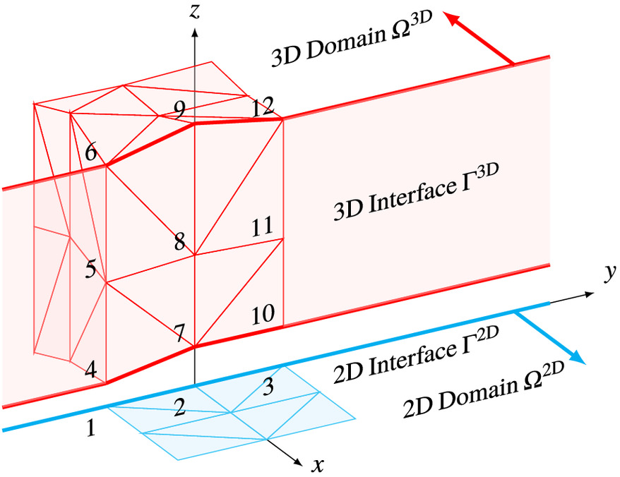
N^{3 D}

denote the sets of all nodes in the 2D and 3D submodels, respectively. The sets of nodes lying on the 2D–3D interface on the 2D and 3D sides as are denoted as

I^{2 D}

and

I^{3 D}

, respectively. The sets of noninterface nodes of the models are therefore given by the set difference

N^{n D} - I^{n D}

,

n \in {2, 3}

. In Fig. 1, for example, the set of 2D model interface nodes is

I^{2 D} = {1, 2, 3}

, whereas the set of 3D model interface nodes is

I^{3 D} = {4, 5, \dots, 12}

. For conformity, the interface nodes must be aligned into node columns as shown so that they have the same horizontal locations. This also results in 1D boundary edges constituting

Γ^{2 D}

being perfectly aligned with columns of 2D boundary faces constituting

Γ^{3 D}

.

In the example shown in Fig. 1, Node 1 is coupled to node Column

C (1) = {4, 5, 6}

, Node 2 to node Column

C (2) = {7, 8, 9}

, and Node 3 to node Column

C (3) = {10, 11, 12}

. Thus, in terms of code implementation, the 2D nodes

I

are coupled to corresponding 3D node columns

C (I)

by enforcing specific relations between solution variables among the coupled nodes. This is done in the HVEL, WVEL, and transport solution stages mentioned in the previous section. The relations enforced between the solution variables within coupled node columns are mutual equality in the case of coupled HVEL and transport solution stages, whereas in the coupled WVEL stage, they are equal only at the bed and surface nodes with linear variation in between.

For example, for the 3D nodes

C (2) = {7, 8, 9}

coupled to the 2D Node 2, the HVEL and transport stages enforce

h_{2}^{2 D} = h_{9}^{3 D}

,

{\bar{u}}_{2}^{2 D} = u_{7}^{3 D} = u_{8}^{3 D} = u_{9}^{3 D}

,

{\bar{v}}_{2}^{2 D} = v_{7}^{3 D} = v_{8}^{3 D} = v_{9}^{3 D}

, and

{\bar{c}}_{2}^{2 D} = c_{7}^{3 D} = c_{8}^{3 D} = c_{9}^{3 D}

, and the WVEL stage enforces

w_{2}^{s, 2 D} = w_{9}^{3 D}

and

w_{2}^{b, 2 D} = w_{7}^{3 D}

, with

w_{8}

chosen so that the vertical velocity is linear over the node column.

Model Requirements for 2D-3D Coupling

Continuity of the solution, mass flux, horizontal momentum fluxes, and constituent fluxes across the 2D–3D interface are enforced at all times in traditional CG-FEMs. For strong coupling, two additional requirements are imposed on the models: the first is on the applicability of the 2D-3D coupled model to enforce its sensible use, and the second is a conformity requirement to ensure discrete conservation of mass and momentum across the 2D–3D interface. The qualitative applicability requirement is a caution on the possible pitfalls of incorrectly using 2D-3D coupled models (irrespective of the type of coupling, strong or weak) whereas the conformity requirement naturally leads to a monolithic 2D-3D coupled system (irrespective of its applicability).

Applicability

An obvious restriction on 2D-3D coupled models is that the interface should be placed in a region where 2D models are accurate. In the case of baroclinic transport simulations, for example, the 2D subdomain and the 2D–3D interface should be placed in a region in which the water is well-mixed vertically throughout the duration of the simulation. Nevertheless, it may be still possible that users of 2D-3D coupled models are forced to place the 2D–3D interface in a baroclinic region due to lack of any other option. In the baroclinic test cases herein, we test the limits of 2D-3D strong coupling by violating the applicability recommendation in order to understand the solution behavior in such scenarios. Because this condition on applicability does not prevent one from coupling 2D and 3D models, it is more of an engineering guideline than an assumption or restriction on 2D-3D coupling.

Conformity

Discrete mass and momentum conservation across element boundaries in the continuous Galerkin FEM is a natural outcome of conformity. The definition of conformity over a mesh essentially requires that the trial space

U^{h}

be a subspace of

H^{1} (Ω)

, which is the space of square integrable functions in

L^{2} (Ω)

such that their first-order derivatives are also in

L^{2} (Ω)

. The conditions for conformity in relation to the

H^{1}

space have been given by Solin et al. (2003). In the case of solely 2D or 3D meshes that use the classical space

U^{h}

of continuous piecewise linear polynomials as the trial space, conformity conditions are satisfied by the manner of construction of basis functions

ϕ_{i} \in U^{h}

. The 2D-3D strong coupling approach herein requires conformity in the coupled models as well.

HVEL and Transport Stage Coupling

As noted in the previous section, the classical trial space of continuous piecewise linear polynomials satisfies the conditions of conformity by construction of a particular basis to define the space. Relying on coupled node columns being aligned vertically and there being no gaps in the coupled interface, an appropriate basis is constructed for the trial space

U_{2 D 3 D}^{h}

of the 2D-3D strongly coupled model as well, starting with the classical trial spaces of the 2D and 3D regions of the hybrid mesh, denoted as

U_{2 D}^{h}

and

U_{3 D}^{h}

, respectively. To that end, let

Ω^{2 D}

and

Ω^{3 D}

denote the 2D and 3D regions of the hybrid 2D-3D domain

Ω^{2 D 3 D} = Ω^{2 D} \cup Ω^{3 D}

, respectively. The sets

N^{2 D}

,

N^{3 D}

,

I^{2 D}

, and

I^{3 D}

are as defined previously. Let

ϕ_{i}^{2 D}

and

ϕ_{i}^{3 D}

be the original, classical hat basis functions, respectively, of

U_{2 D}^{h} (Ω^{2 D})

and

U_{3 D}^{h} (Ω^{3 D})

, defined as continuous piecewise linear functions with

ϕ_{i} (x_{j}) = δ_{i j}

, where

i

is the node corresponding to the basis function

ϕ_{i}

,

x_{j}

is the location of any node

j

in the respective mesh, and

δ_{i j}

is the Kröenecker delta function with a value of one if

i = j

and zero otherwise.

The construction of the basis functions for

U_{2 D 3 D}^{h} (Ω^{2 D 3 D})

begins with defining intermediate functions

ι_{i}^{2 D}, ι_{i}^{3 D} : Ω^{2 D 3 D} \to R

as trivial extensions of

ϕ_{i}^{2 D}

and

ϕ_{i}^{3 D}

corresponding to all nodes

i \in N^{2 D}

and

i \in N^{3 D}

of the parent meshes onto the entire coupled domain

Ω^{2 D 3 D}

, written

ι_{i}^{2 D} (x) = {\begin{cases} ϕ_{i}^{2 D} (x), & x \in Ω^{2 D} \\ 0, & x \in Ω^{3 D} \end{cases}, \forall i \in N^{2 D} ι_{i}^{3 D} (x) = {\begin{cases} 0, & x \in Ω^{2 D} \\ ϕ_{i}^{3 D} (x), & x \in Ω^{3 D} \end{cases}, \forall i \in N^{3 D}

(18)

The intermediate functions corresponding to the noninterface nodes

i \in N^{2 D} - I^{2 D}

or

i \in N^{3 D} - I^{3 D}

in the coupled domain are continuous throughout and satisfy the conditions of conformity by default. It is the intermediate functions at the 2D–3D interface nodes

i \in I^{2 D}

or

i \in I^{3 D}

that are discontinuous. Using these intermediate functions, however, functions continuous across the 2D–3D interface, to be included in the basis, are constructed. The number of basis functions at the 2D–3D interface is the same as the number of sets of coupled nodes at the interface, which is

| I^{2 D} |

. The final basis functions

ϕ_{i}^{2 D 3 D} \in U_{2 D 3 D}^{h} (Ω^{2 D 3 D})

can be defined

ϕ_{i}^{2 D 3 D} = {\begin{cases} ι_{i}^{2 D}, & \forall i \in N^{2 D} - I^{2 D} \\ ι_{i}^{3 D}, & \forall i \in N^{3 D} - I^{3 D} \\ ι_{i}^{2 D} + \sum_{j \in C (i)} ι_{j}^{3 D}, & \forall i \in I^{2 D} \end{cases}

(19)

where continuity of

ϕ_{i}^{2 D 3 D} \forall i \in I^{2 D}

is guaranteed by the depth-summability property of the basis functions Eq. (12). This property ensures that from Eqs. (18) and (12), depth-summing

ϕ_{j}^{3 D}

over coupled node columns

C (i)

would result in the function

ϕ_{I}

on the 3D side, where

I

is the 2D node that generates the node column

C (I)

on extrusion, which is the 2D interface node

i

itself. The function

ϕ_{I} \cup ϕ_{i}^{2 D}

, obtained by joining

ϕ_{I}

and

ϕ_{i}^{2 D}

, is a basis function of the original full-2D mesh from which the 2D-3D hybrid mesh is generated and is continuous by construction. In particular

ι_{i}^{2 D} |_{Γ^{2 D}} (x) = (\sum_{j \in C (i)} ι_{j}^{3 D}) |_{Γ^{3 D}} (x), \forall i \in I^{2 D}, \forall x \in Γ

(20)

The functions

ϕ_{i}^{2 D 3 D}

satisfy the conditions for conformity (Choudhary 2019). The test spaces are defined analogously as in Eq. (19), with the trial functions replaced with test functions.

The functions in Eq. (19) satisfy conformity and also form a basis on the space

U_{2 D 3 D}^{h}

by construction. The space is complete, and therefore all functions

f

in the constructed space satisfy conformity. Hence, the 2D-3D strongly coupled models presented herein are conforming. The aforementioned steps apply for HVEL and transport stages of the 2D-3D strongly coupled models. The solution variables

{h^{3 D}, u^{3 D}, v^{3 D}, c^{3 D}}

on the 3D side and

{h^{2 D}, {\bar{u}}^{2 D}, {\bar{v}}^{2 D}, {\bar{c}}^{2 D}}

on the 2D side are defined using the trial basis Eq. (19). There is no ambiguity at the 2D–3D interface due to conformity, which ensures that the solution at the interface is continuous and single-valued. Due to the nature of the trial functions, the HVEL/transport solution variables on the 2D and 3D sides of the interface are effectively set to be node-columnwise equal.

WVEL Stage Coupling

The WVEL stage coupling is only slightly different compared with the HVEL and transport coupling stages because the vertical velocity can be nonconstant along the

z

-direction. Moreover, because two equations per node are available on the 2D side for the WVEL stage given by Eq. (17), enforcing linear variation of

w

along the

z

-direction becomes possible. Because the WVEL coupling method is still similar to that of the HVEL stage and an example has been presented in the “Background Definitions” section, the mathematical details of the WVEL stage coupling are not presented herein [Choudhary (2019) has given complete details].

Conservation across the 2D–3D Interface

As in the case of solely 2D or 3D models, discrete conservation across the 2D–3D interface is a natural consequence of conformity. Because the meshes on the sides of the 2D–3D interface are of different dimensions, the strictest level of conservation of quantities in the continuous sense would be columnwise, i.e., vertically integrated quantities would have to be conserved ideally at every horizontal location

x = (x, y) \in Γ^{2 D}

. This can be stated as follows:

(\begin{array}{c} h^{2 D} \\ h^{2 D} {\bar{u}}^{2 D} \\ h^{2 D} {\bar{v}}^{2 D} \\ h^{2 D} {\bar{c}}^{2 D} \end{array}) {\bar{u}}^{2 D} \cdot n^{2 D} = - \int_{b^{3 D}}^{η^{3 D}} (\begin{array}{c} 1 \\ u^{3 D} \\ v^{3 D} \\ c^{3 D} \end{array}) u^{3 D} \cdot n^{3 D} d z

(21)

for all

(x, y) \in Γ^{2 D}

, where

n

= normal facing outward from the respective domain. Here, each solution variable has been tagged as 2D or 3D to make it clear which side of the 2D–3D interface it comes from. It can also be shown using Eqs. (19) and (20) that

ϕ_{K}^{2 D} (\begin{array}{c} h^{2 D} \\ h^{2 D} {\bar{u}}^{2 D} \\ h^{2 D} {\bar{v}}^{2 D} \\ h^{2 D} {\bar{c}}^{2 D} \end{array}) {\bar{u}}^{2 D} \cdot n^{2 D} = - \sum_{i \in C (K)} \int_{b^{3 D}}^{η^{3 D}} ϕ_{i}^{3 D} (\begin{array}{c} 1 \\ u^{3 D} \\ v^{3 D} \\ c^{3 D} \end{array}) u^{3 D} \cdot n^{3 D} d z

(22)

for all

(x, y) \in Γ^{2 D}

and

K \in I^{2 D}

. This gives conservation on the discrete level, which is less strict and requires that for all

K \in I^{2 D}

\int_{Γ^{2 D}} ϕ_{K}^{2 D} (\begin{array}{c} h^{2 D} \\ h^{2 D} {\bar{u}}^{2 D} \\ h^{2 D} {\bar{v}}^{2 D} \\ h^{2 D} {\bar{c}}^{2 D} \end{array}) {\bar{u}}^{2 D} \cdot n^{2 D} d Γ^{2 D} = - \sum_{i \in C (K)} \int_{Γ^{3 D}} ϕ_{i}^{3 D} (\begin{array}{c} 1 \\ u^{3 D} \\ v^{3 D} \\ c^{3 D} \end{array}) u^{3 D} \cdot n^{3 D} d Γ^{3 D}

(23)

Here, there are four equations corresponding to mass, horizontal momentum, and constituent conservation across the interface. The following facts ensure that all the aforementioned conservation conditions are satisfied in case of the strongly coupled models presented herein:

1.

For all points

x

on the 2D–3D interface

Γ

,

n^{3 D} (x) = - n^{2 D} (x)

holds for the outward pointing normals independent of

z

because there are no gaps in the 2D–3D interface.

2.

The solution variables

u^{3 D}

,

v^{3 D}

, and

c^{3 D}

are independent of

z

at the 2D–3D interface by the choice of the trial function.

3.

Although

w^{3 D}

is

z

-dependent, its contribution in

u^{3 D} \cdot n^{3 D}

is zero because the normal at the 2D–3D interface is orthogonal to the

z

-direction.

4.

Conformity implies that

{ϕ_{K}^{2 D} |}_{Γ^{2 D}} = (\sum_{i \in C (K)} ϕ_{i}^{3 D}) |_{Γ^{3 D}}

holds.

Verification of 2D-3D Coupling

Small-Amplitude Slosh Test Case

The slosh or seiche test case is a common test case for SW models investigating wave propagation (Wang et al. 2008). In this case, water is filled in a rectangular domain given by

Ω = (0, L) \times (0, W)

, where the length

L

and width

W

are 25.6 and 6.4 km, respectively. The bed elevation is

b (x, y) = - H = - 82.5 m

, and the at-rest water depth is

H

, corresponding to a water surface elevation of 0 m. Density is constant at

990 kg / m^{3}

throughout the domain, and the total volume of fluid contained in the domain is

L \times W \times H = 13.5168 {km}^{3}

. The boundary conditions specified on all vertical boundaries are no-normal-flow, i.e.,

u \cdot n = 0

. The water is initially at rest throughout the domain. An initial condition on the depth is specified, given by

h (x, y, 0) = H + a \cos (π x / L)

(24)

which is a right-left varying perturbation in the form of a cosine wave of amplitude

a = 0.01 m

and wavelength

2 L

. There is no viscosity, bottom friction, wind, or air pressure.

The 2D and 3D linearized systems have the same analytical solution (Wang et al. 2008)

h^{lin} (x, y, t) = H + a \cos (\frac{π}{L} x) \cos (\frac{π \sqrt{g H}}{L} t) u^{lin} (x, y, z, t) = \frac{a \sqrt{g H}}{H} \sin (\frac{π}{L} x) \sin (\frac{π \sqrt{g H}}{L} t) v^{lin} (x, y, z, t) = 0 w^{lin} (x, y, z, t) = - (\frac{a π \sqrt{g H}}{L}) (\frac{z - b}{H}) \cos (\frac{π}{L} x) \sin (\frac{π \sqrt{g H}}{L} t)

(25)

This analytical solution is not the analytical solution to the full nonlinear SWEs solved by AdH. Hereafter, the unknown analytical solution of the full nonlinear SWE is referred to as the true solution, the finest-mesh, smallest-time-step FE solution is called the converged FE solution, the solution Eq. (25) to the linearized SWE is the analytical solution, and any other mesh/time-step solution is referred to as a finite-element (FE) solution in order to distinguish among them. The true, converged FE, analytical, and FE solutions are denoted by

s = (h, u)

,

\tilde{s} = (\tilde{h}, \tilde{u})

,

s^{lin} = (h^{lin}, u^{lin})

, and

s^{h} = (h^{h}, u^{h})

, respectively.

Error Definitions

In order to analyze the error plots and convergence results, additional terminology is introduced. The temporally varying spatial

L^{2}

norm for a scalar

f = f (x, t)

and a vector

v = v (x, t)

is defined

∥ f ∥^{2} (t) = \int_{Ω} f^{2} d Ω, ∥ v ∥^{2} (t) = \int_{Ω} (v \cdot v) d Ω

(26)

Instead of computing the actual integral, the root-mean square (RMS) error of nodal values is used for convergence analysis because it is an approximation of the

L^{2}

norm by a fixed domain-dependent factor and is sufficient for obtaining convergence rates (Choudhary 2019). The FE solution errors are defined

e^{h} = {e_{h}^{h}, e_{u}^{h}} = {h - h^{h}, u - u^{h}} = s - s^{h}

(27a)

e^{lin, h} = {e_{h}^{lin, h}, e_{u}^{lin, h}} = {h^{lin} - h^{h}, u^{lin} - u^{h}} = s^{lin} - s^{h}

(27b)

{\tilde{e}}^{h} = {{\tilde{e}}_{h}^{h}, {\tilde{e}}_{u}^{h}} = {\tilde{h} - h^{h}, \tilde{u} - u^{h}} = \tilde{s} - s^{h}

(27c)

These functions depend on the mesh size,

h

, and the time step,

Δ t

. On the other hand, the (unknown) method-,

h

-, and

Δ t

-independent difference between the true and analytical solutions is defined

e^{lin} = {e_{h}^{lin}, e_{u}^{lin}} = {h - h^{lin}, u - u^{lin}} = s - s^{lin}

(27d)

Although the converged FE solution,

\tilde{s}

, depends on the mesh and time step sizes, it can be considered as

h

- and

Δ t

-independent for a sufficiently fine mesh using a sufficiently small time step. Therefore, the error between the true solution and the converged FE solution is defined

\tilde{e} = {{\tilde{e}}_{h}, {\tilde{e}}_{u}} = {h - \tilde{h}, u - \tilde{u}} = s - \tilde{s}

(27e)

and is treated as if it is

h

- and

Δ t

-independent. Lastly, the error between the analytical solution and the true solution can be approximated using the error between the converged FE solution and the analytical solution, defined

{\tilde{e}}^{lin} = {{\tilde{e}}_{h}^{lin}, {\tilde{e}}_{u}^{lin}} = {\tilde{h} - h^{lin}, \tilde{u} - u^{lin}} = \tilde{s} - s^{lin}

(27f)

In general, convergence behavior should be analyzed by calculating

e^{h}

, which is unknown in this case because the true solution

s

is unknown. The quantities that can be calculated are

e^{lin, h}

,

{\tilde{e}}^{h}

, and

{\tilde{e}}^{lin}

. Both

e^{lin, h}

and

{\tilde{e}}^{h}

are approximations to

e^{h}

, whereas

{\tilde{e}}^{lin}

approximates

e^{lin}

. For both temporal and spatial convergence analyses, the maximum-over-time values of the calculable RMS errors are defined

E_{h}^{lin, h} = \max_{t \in [0, T]} ∥ e_{h}^{lin, h} ∥, {\tilde{E}}_{h}^{h} = \max_{t \in [0, T]} ∥ {\tilde{e}}_{h}^{h} ∥, {\tilde{E}}_{h}^{lin} = \max_{t \in [0, T]} ∥ {\tilde{e}}_{h}^{lin} ∥ E_{u}^{lin, h} = \max_{t \in [0, T]} ∥ e_{u}^{lin, h} ∥, {\tilde{E}}_{u}^{h} = \max_{t \in [0, T]} ∥ {\tilde{e}}_{u}^{h} ∥, {\tilde{E}}_{u}^{lin} = \max_{t \in [0, T]} ∥ {\tilde{e}}_{u}^{lin} ∥

(28)

Model Parameters

The results of the 2D-3D coupled model are compared with equivalent full-2D and full-3D models. In the 2D-3D coupled model, the right portion of the domain is the 3D model and the left part is the 2D model, with the 2D–3D interface located at

x = L / 2 = 12.8 km

. The total simulation time was set to 3 h, corresponding to six oscillation cycles. The time period of sinusoidal oscillations in the domain, according to Eq. (25) with

g = 9.81 m / s^{2}

is

2 L / \sqrt{g H} = 1799.7 s

, or nearly 0.5 h. The converged FE solution,

\tilde{s}

, is set to be the FE solution of a model with mesh

size = 50 m

and time

step = 1 s

, which is the finest mesh and smallest time step chosen for this test case.

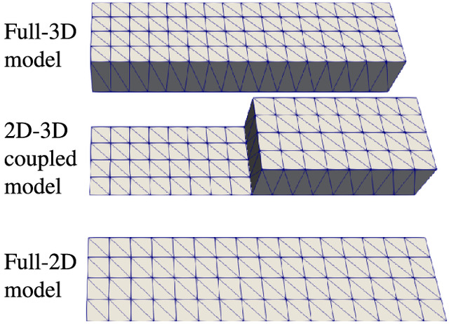
For spatial convergence, the FE solutions,

s^{h}

, of seven coarser meshes with horizontal node spacing

h = Δ x = Δ y = {6,400, 3,200, 1,600, 800, 400, 200, 100} m

were used. The full-2D, 2D-3D coupled, and full-3D meshes are shown in Fig. 2 for the case of

h = 1,600 m

. In all 3D models, a single layer of elements was used in the vertical direction, and the meshes were refined only in the horizontal plane. For the spatial convergence analysis, second-order time stepping was used with a time step of 1 s, determined after temporal convergence analysis in order to reduce time discretization errors.

Fig. 2. Slosh test case meshes $Δ x = Δ y = 1,600 m$ (scaled by a factor of 50 in the $z$ -direction).

For temporal convergence, the second finest mesh (

Δ x = Δ y = 100 m

) was used, with time step sizes

Δ t = {30, 15, 10, 6, 3, 1} s

, so that time discretization errors dominated the mesh discretization errors, allowing extraction of temporal convergence rates. The results of simulations using 3- and 1-s time steps should be excluded for obtaining temporal convergence rates because the converged FE solution should have been obtained using an even smaller time step and finer mesh for these.

For the spatial convergence analysis, two sets of simulations were run, one excluding and including the SUPG terms. For low amplitudes, the simulations excluding SUPG terms ran successfully without resulting in the typical node-to-node oscillations usually seen in advection-dominated problems. The maximum-over-time errors with respect to the analytical and converged FE solutions, i.e.,

{E_{h}^{lin, h}, E_{u}^{lin, h}}

and

{{\tilde{E}}_{h}^{h}, {\tilde{E}}_{u}^{h}}

, were used for the convergence analysis, and the units of the errors dropped. The maximum-over-time value of the method-,

h

-, and

Δ t

-independent RMS errors of the analytical solution with respect to the converged FE solution,

{\tilde{E}}_{h}^{lin}

and

{\tilde{E}}_{u}^{lin}

for all models were observed to be in the following range:

{\tilde{E}}_{h}^{lin} \approx (1.4 \pm 0.2) \times 10^{- 5} {\tilde{E}}_{u}^{lin} \approx (5 \pm 1) \times 10^{- 6}

(29)

Temporal Convergence

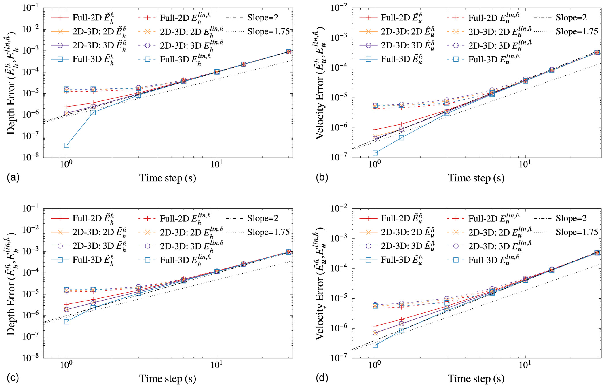
For the temporal convergence analysis, the errors

e^{lin, h}

and

{\tilde{e}}^{h}

of the finite-element solutions

s^{h}

of the second finest mesh of size 100 m and time steps

Δ t = {30, 15, 10, 6, 3, 1} s

were used. Fig. 3 plots the RMS errors of depth and velocity versus time step for the full-2D, 2D-3D and full-3D models with the top and bottom subfigures respectively corresponding to simulations excluding and including SUPG terms. The dashed lines in the figures correspond to errors with respect to

s^{lin}

, and the solid lines are for comparison against

\tilde{s}

. When comparing against the analytical solution

s^{lin}

, the errors flatten out to the values given by Eq. (29) on time step refinement, as expected. Excluding two of the leftmost points in the figures, the temporal convergence rate using comparison with

\tilde{s}

is seen to be second order as expected.

Fig. 3. Small-amplitude slosh test of temporal convergence using Mesh 7 and $h = 100 m$ : (a) depth error convergence excluding SUPG terms; (b) velocity error convergence excluding SUPG terms; (c) depth error convergence including SUPG terms; and (d) velocity error convergence including SUPG terms.

Spatial Convergence

Next, we compared errors against the converged FE solution corresponding to the mesh size 50 m and time

step = 1 s

. The errors

∥ {\tilde{e}}^{h} ∥

of the remaining seven meshes against the converged FE solution,

\tilde{s}

, were obtained, and

{\tilde{E}}_{h}^{h}

and

{\tilde{E}}_{u}^{h}

were calculated. For comparison with respect to the analytical solution to the linearized SWEs, all eight meshes were used to calculate

E_{h}^{lin, h}

and

E_{u}^{lin, h}

, noting that for the eighth mesh with mesh

size = 50 m

, these are, respectively,

{\tilde{E}}_{h}^{lin}

and

{\tilde{E}}_{u}^{lin}

given by Eq. (29).

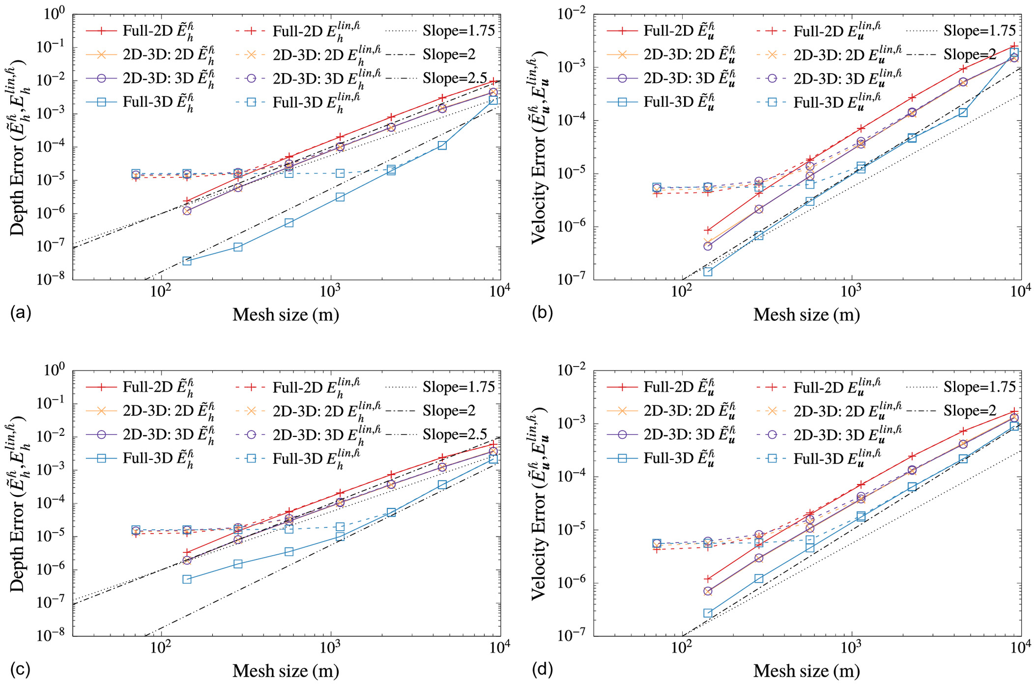
Spatial convergence plots for depth and velocity magnitude are shown in Fig. 4. The dashed and solid lines in the figures correspond to RMS error comparison against the analytical and converged FE solutions, and the subfigures on the top and bottom, respectively, correspond to simulations with SUPG terms excluded and included during simulations. Following are the observations from the four convergence plots:

•

The errors of the 2D-3D coupled models are seen to lie between those of the full-2D and full-3D models for all mesh sizes.

•

From Figs. 4(a and b) for simulations excluding SUPG terms, the spatial convergence rates for all three models are observed to be second order for depth as well as velocity, with the exception of depth in the full-3D model, which converged at an even higher rate of 2.5.

•

From Figs. 4(c and d) for simulations including SUPG terms, the spatial convergence rates for all three models are observed to be nearly second order for depth as well as velocity.

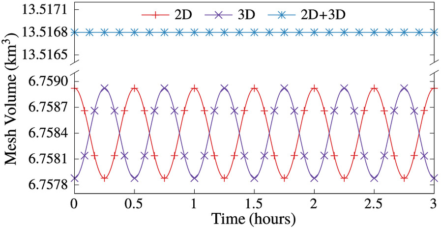
Fig. 4. Small-amplitude slosh test of spatial convergence using $Δ t = 1 s$ : (a) depth error convergence excluding SUPG terms; (b) velocity error convergence excluding SUPG terms; (c) depth error convergence including SUPG terms; and (d) velocity error convergence including SUPG terms.

Mass Conservation across the 2D–3D Interface

Fig. 5 shows the volume of water in the individual 2D and 3D submodels along with the total volume over a period of 3 hours for the sixth mesh of size

h = 200 m

. It is seen from the figure that the individual volumes change with time as expected, but the total volume of water remains constant at

13.5168 {km}^{3}

, verifying global mass conservation, and in turn, conservation of mass as water moves across the interface.

Fig. 5. Small-amplitude slosh test: verification of conservation of mass in 2D-3D coupled models using the sixth mesh, $h = 200 m$ .

Baroclinic Flume Test Case

Salt water-freshwater mixing is fundamental in estuarine dynamics research (Xia et al. 2019). In this test case, baroclinic flow in a rectangular domain was simulated, which violates the recommendation of keeping the 2D–3D interface away from baroclinic regions, explained in the section “Strongly Coupled 2D and 3D Shallow Water Models.” The purpose of this test is to observe the behavior of baroclinicity close to the 2D–3D interface because it may not always be practical to keep the 2D–3D interface away from baroclinic regions. In order to isolate interfacial errors to the coupling method only, errors from advection instabilities were minimized by introducing a small shock with a low salinity inflow. Also, a large purpose of this test case was to show what kind of numerical artifacts arise from improper interface positions.

The rectangular domain used in this test case is given by

Ω = (0, 3.2) \times (0, 0.2) km

. The bed elevation was

b (x, y) = - H = - 10 m

. The water was initially at rest with a constant depth of

H = 10 m

and salinity of

0 g / kg

. The north and south boundaries of the models,

y = {0, 0.2} km

, had a no-normal-flow boundary condition. An inflow of

Q = 400 m^{3} / s

with a salinity of

1 g / kg

was specified on the western boundary at

x = 0 km

. The water surface elevation at the eastern boundary,

x = 3.2 km

, was fixed at 0 m. There was no bottom friction, wind, or air pressure.

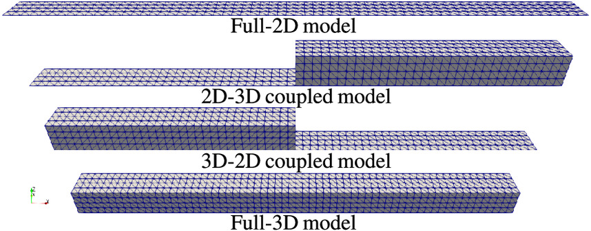
The meshes for this case are shown in Fig. 6. The first 2D-3D coupled model has the 2D subdomain located on the left side and the 3D subdomain on the right. The second 2D-3D coupled model has the opposite placement of the 2D and 3D subdomains. The models are, respectively, referred to as 2D-3D and 3D-2D coupled models in this section. For both the models, the coupling interface was placed midway along the length at

x = 1.6 km

. The horizontal node spacing was

Δ x = Δ y = 50 m

, and in case of all 3D submodels, the vertical node spacing was

Δ z = 0.025 m

, corresponding to a vertical resolution of four element layers. The Smagorinsky coefficient was set to 0.2. A time step of 300 s was used for the simulation, and the simulation ending time was set to 4 h.

Fig. 6. Baroclinic flume test case meshes $Δ x = Δ y = 50 m$ and $Δ z = 2.5 m$ (scaled by a factor of 20 in the $z$ -direction).

Because the water was initially at rest and fresh, transient oscillations were initially seen at the saline boundary front. These oscillations were damped quickly due to the use of first-order time stepping, a larger time step, and viscosity. Also, because the domain initially had freshwater and the water flowing into the domain was saline, a salinity front travels across the domain from west to east. The steady-state solution is a constant water depth of 10 m, uniform horizontal velocity of

0.2 m / s

in the

x

-direction, and a uniform salinity of

1 g / kg

.

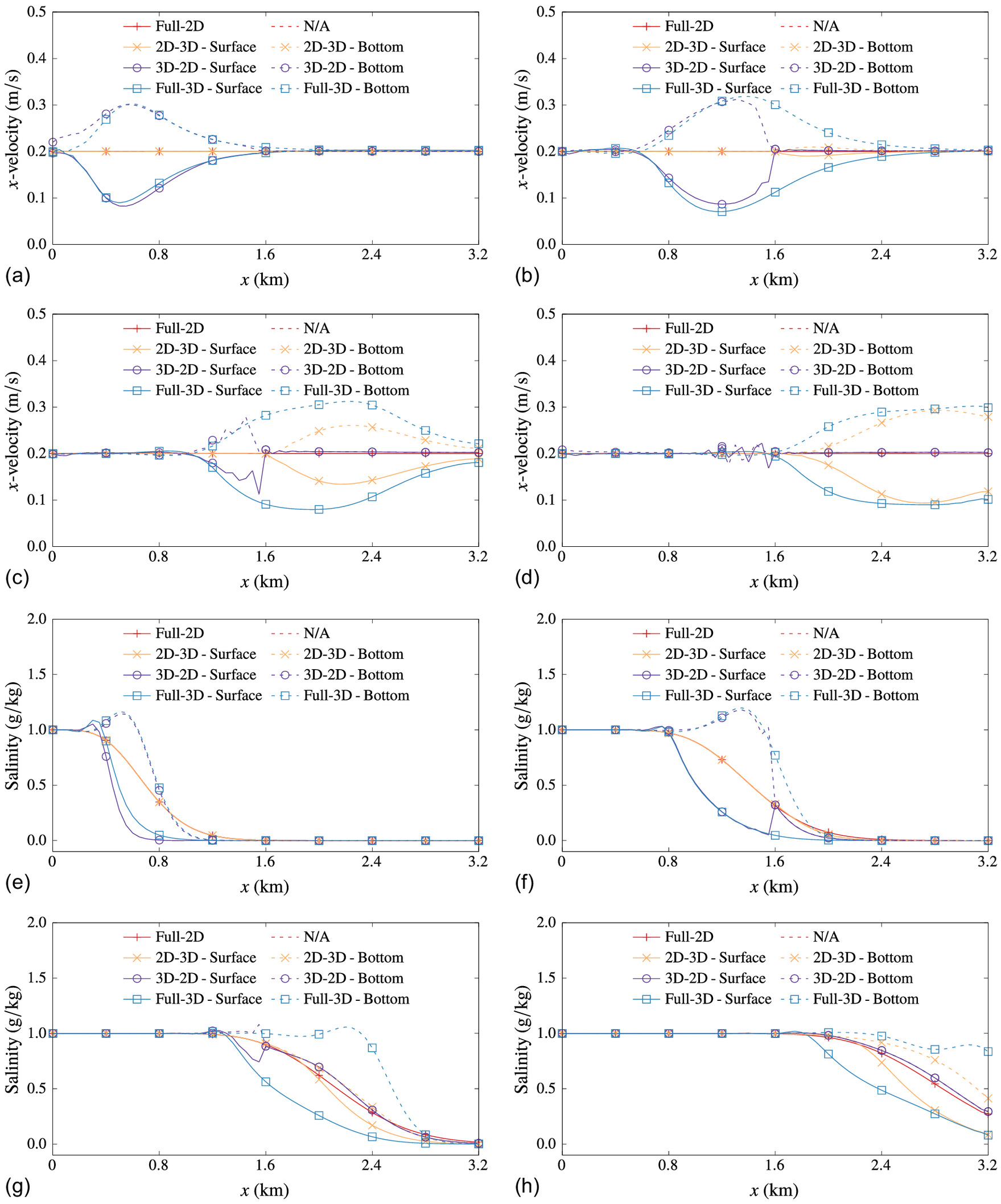
Fig. 7 shows the

x

-velocity and salinity in the models at hourly intervals. These are depth-averaged values in case of 2D submodels, and surface (solid) and bed (dashed) values in case of 3D submodels. Due to baroclinicity, the denser saline water sinks, and salinity and

x

-velocity shocks travel along the bed in the full-3D and coupled domains, seen by a separation of the dashed and solid lines in all the figures. The observations from Fig. 7 can be divided temporally into three stages:

•

Initial stage: The salinity front just entered the domains and was still far away from the coupling interface. From Figs. 7(a and e), it is observed that the 2D-3D coupled model initially behaved like the full-2D model, whereas the 3D-2D coupled model initially behaved like the full-3D model.

•

Intermediate stage: The salinity front was in the vicinity of the coupling interface, before, during, and after crossing it. From Figs. 7(b, c, f, and g), it is observed that the coupled models were in a state of transition. In the 2D-3D coupled model, the transition of the salinity and

x

-velocity front from the 2D domain was smooth. In the 3D-2D coupled model, however, the movement of the stratified salinity and

x

-velocity front from the 3D domain into the 2D domain resulted in temporary oscillatory behavior in the velocity (but not in the salinity, or the depth which is not shown here). This is precisely the reason why it is important to place the coupling interface away from baroclinic areas. In a practical scenario, however, that may not always be possible, in which case the oscillations can be damped by increasing stabilization in the 3D elements close to the 2D–3D interface. When the salinity front reached the interface, the salinity near the surface was about

0 g / kg

, whereas that near the bed was close to

1 g / kg

. Likewise, the

x

-velocity was also stratified. The 2D-3D coupling forced the solution to be constant down a node column, which prevented the salinity and

x

-velocity front from staying stratified when crossing the interface. This resulted in a change in the velocities and salinity close to the interface, and as observed here, may lead to oscillations.

•

Final stage: The salinity front fully crossed the coupling interface and was reasonably far away from it. From Figs. 7(d and h), it is observed that the situation has flipped in comparison with the initial stage, i.e., the 2D-3D coupled model now behaved like the full-3D model, whereas the 3D-2D model behaved like the full-2D model. Also, all the models attained the correct steady-state solution on running them for a longer time, which is not shown here. The oscillations in the 3D-2D coupled model were also gone once the salinity front crossed the coupling interface.

Fig. 7. Baroclinic flume test showing $x$ -velocity and salinity in the full-2D, 2D-3D coupled, 3D-2D coupled, and full-3D models at different time stamps: (a) $x$ -velocity at $t = 1 h$ ; (b) $x$ -velocity at $t = 2 h$ ; (c) $x$ -velocity at $t = 3 h$ ; (d) $x$ -velocity at $t = 4 h$ ; (e) salinity at $t = 1 h$ ; (f) salinity at $t = 2 h$ ; (g) salinity at $t = 3 h$ ; and (h) salinity at $t = 4 h$ .

Lock-Exchange Test Case

Another extreme case of baroclinicity, the lock-exchange experiment, was used to observe the behavior of coupled models with respect to full-2D and full-3D models. This is a common analytical test for the accuracy of the shock speed of a density wedge. In a lock exchange experiment, fluids of different densities initially at rest are separated by a vertical barrier, called the lock gate, in a tank (Shin et al. 2004). As is the case with the baroclinic flume test case, this case also violates the recommendation of placing the 2D–3D interface away from baroclinic areas. For this test case, the rectangular domain is given by

Ω = (- 1, 1) \times (- 0.1, 0.1) \times (- 0.2, 0.0) m

. The initial condition was water at rest with a constant water depth of

h (x, y, 0) = H = 0.2 m

with a initial salinities of

30.0 g / kg

for

x \in (- 1, 0) m

and

10.0 g / kg

for

x \in (0, 1) m

. All the vertical boundaries had the no-normal-flow Neumann boundary condition,

u \cdot n = 0

. The horizontal spacing of nodes in the meshes was

Δ x = Δ y = 0.05 m

, and in case of 3D submodels, the vertical node spacing was

Δ z = 0.025 m

, corresponding to a vertical resolution of eight element layers.

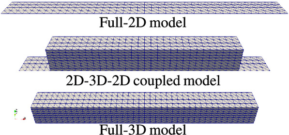
The results of a 2D-3D-2D coupled model were compared with those of full-2D and full-3D models. The 2D-3D-2D coupled model contains one 3D submodel coupled to two 2D submodels on its sides. The 3D submodel corresponds to three-quarters of the domain length,

x \in (- 0.75, 0.75) m

, and the two 2D submodels correspond to

x \in (- 1.0, - 0.75) m

and

x \in (0.75, 1.0) m

, respectively. The meshes of the models are shown in Fig. 8.

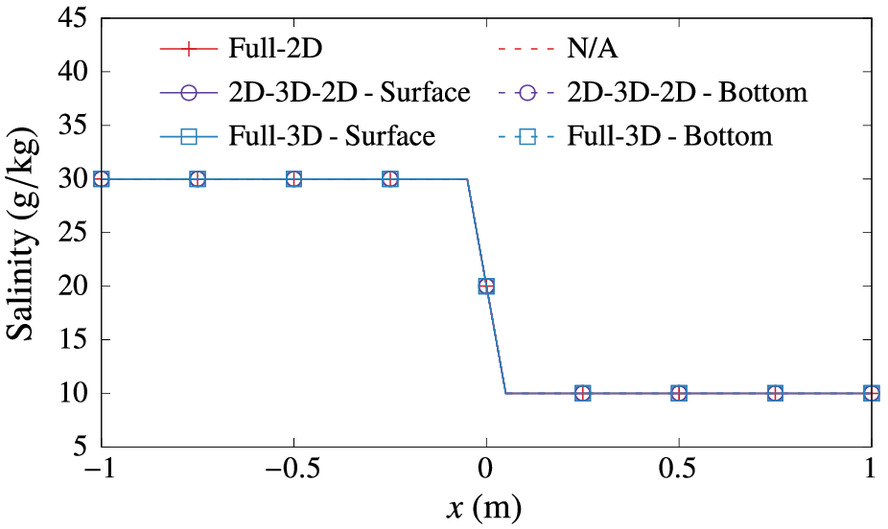
Fig. 8. Lock-exchange test case meshes, $Δ x = Δ y = 0.05 m$ and $Δ z = 0.025 m$ .

For this test case, the Manning’s bottom friction coefficient was set to 0.0015, and the Smagorinsky coefficient was set to 0.2. The salinity diffusivity constant was set to

1 \times 10^{- 5} m^{2} / s

. The salinity dropped from

30 g / kg

on the left to

10 g / kg

on the right across two element layers around

x = 0 m

, as shown in Fig. 9. A time step of 0.5 s was used, and the simulation was run for 48 s. Mesh adaptivity in AdH was turned on, allowing maximum of two levels of mesh refinement.

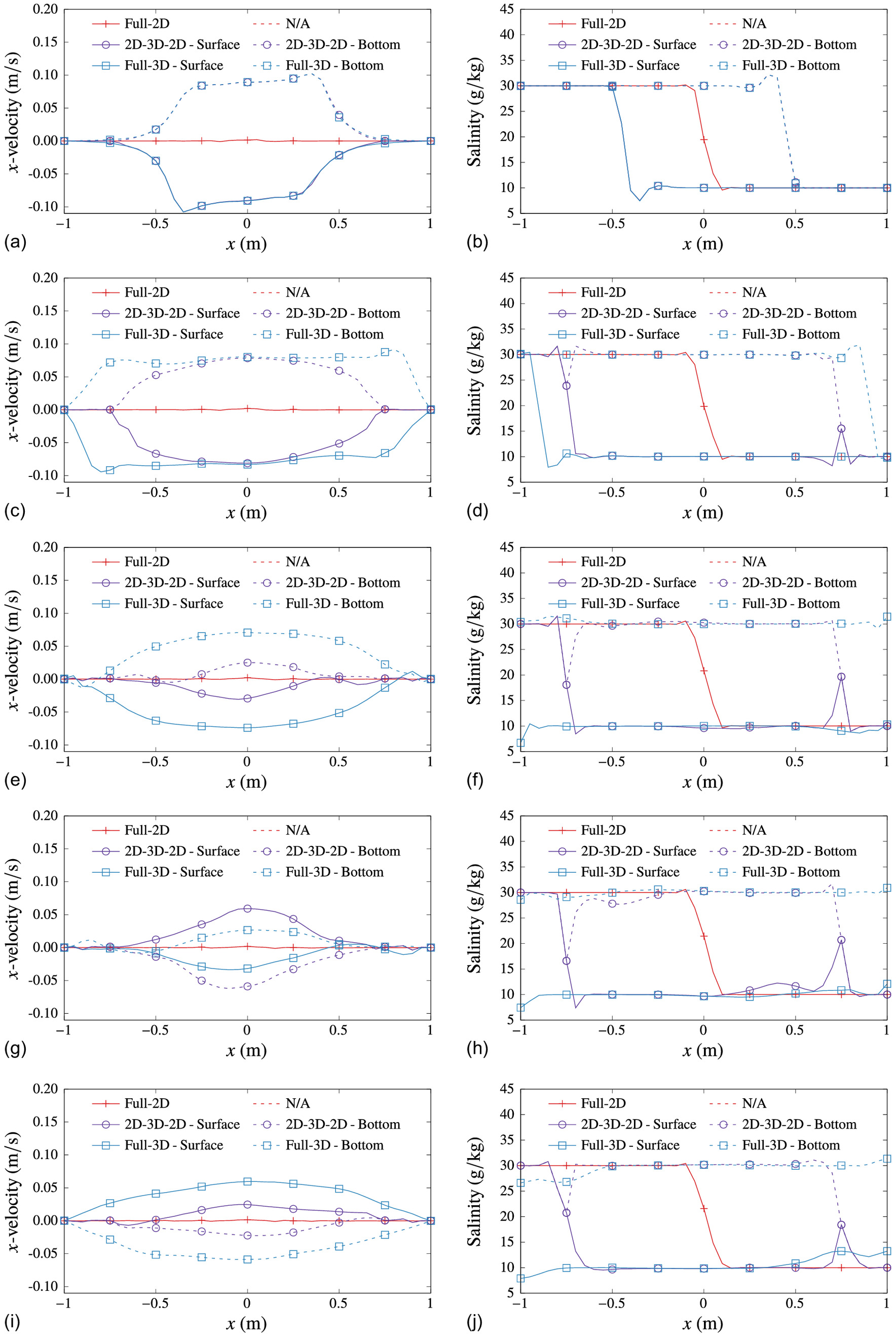
Fig. 9. Lock-exchange test: initial condition on salinity in the full-2D, 2D-3D-2D coupled, and full-3D models.

Figs. 10(a–j) show the variation of

x

-velocity and salinity in the models at time intervals of 8 s except for

t = 40 s

. In the 2D submodels, the plots show depth-averaged values, whereas in case of 3D submodels, the plots show the surface (solid) and bed (dashed) solutions. The subfigures on the top of each page show the

x

-velocity, and those on the bottom show the salinity. The following observations were made from the plots:

•

The full-2D model failed to capture baroclinicity, as expected. Because of this, the solution in the full-2D model stayed nearly the same as the initial condition throughout the simulation.

•

Initially, when the velocity and salinity shocks were a still far away from both the 2D–3D interfaces, the full-3D and the 2D-3D-2D coupled solutions were nearly identical, which they should be, as observed in Figs. 10(a and b).

•

When the stratified shocks reached the 2D–3D interfaces in the 2D-3D-2D coupled models, they did not pass through in this case because 2D-3D coupling enforces a constant solution down a column of nodes, preventing stratification at the interface. It is observed from Figs. 10(c and d) that the 2D-3D-2D coupled solution now fell between the full-2D and the full-3D solution (in say, the

L^{2}

sense and not pointwise).

•

In Figs. 10(e–h), the shocks were observed to be in the process of reflection at the domain boundary in case of the full-3D model and at the 2D–3D interfaces in case of the 2D-3D-2D coupled models. This can be seen as a change in sign in the

x

-velocity.

•

In Figs. 10(i and j), the shocks have reflected, as evident from the bumps in salinity graphs near the domain boundary in case of the full-3D model and the 2D–3D interfaces in the case of the 2D-3D-2D coupled model.

•

The salinity fronts remained stationary at the 2D–3D interfaces on reaching there in the 2D-3D-2D model, and the

x

-velocity in the 2D subdomains remained relatively close to zero. In this case, the 2D–3D interfaces effectively acted as walls where the velocity and salinity shocks were reflected from instead of passing through. This contrasts with the baroclinic flume test case from the previous section, in which the salinity front was forced to cross the interface due to the general nonzero average horizontal flow of water across the 2D–3D interface.

Fig. 10. Lock-exchange test comparison of solutions in the full-2D, 2D-3D-2D coupled, and full-3D models at different time stamps: (a) $x$ -velocity at $t = 8 s$ ; (b) salinity at $t = 8 s$ ; (c) $x$ -velocity at $t = 16 s$ ; (d) salinity at $t = 16 s$ ; (e) $x$ -velocity at $t = 24 s$ ; (f) salinity at $t = 24 s$ ; (g) $x$ -velocity at $t = 32 s$ ; (h) salinity at $t = 32 s$ ; (i) $x$ -velocity at $t = 48 s$ ; and (j) salinity at $t = 48 s$ .

Discussion and Conclusions

In this study, we presented the mathematical formulation and verification of a novel and conservative method for monolithic/strong coupling of 2D-3D shallow water and transport implicit and adaptive CG-FEM SUPG models. Conformity guarantees continuity of solution and conservation of mass and momentum across the 2D–3D coupling interface at all locations and at all times. Three verification test cases were presented, and conservation of mass across the 2D–3D interface was verified in the small-amplitude slosh test case.

For the small-amplitude slosh test case using second-order implicit time stepping, the

L^{2}

error temporal convergence rates of full-2D, 2D-3D coupled, and full-3D models were verified to be second order. The

L^{2}

error spatial convergence rates of all the models with SUPG terms excluded were also observed to be optimal at second order. For simulations with SUPG terms included, the spatial convergence rates for all the models were observed to be slightly lower. The error norms of the 2D-3D coupled models were observed to lie between those of full-2D and full-3D models for most of the time steps in all the meshes for the small-amplitude slosh test case.

Limits of 2D-3D coupled models were tested in baroclinic scenarios violating the base recommendation of placing the 2D–3D interface far away from baroclinicity. In the baroclinic flume test case, 2D-3D and 3D-2D coupled models were compared with full-2D and full-3D models. The salinity front was seen to pass smoothly across the interface into the 3D region from the 2D subdomain in the 2D-3D coupled model. However, temporary velocity oscillations were seen in the 3D-2D coupled model, in which the stratified salinity front passing from the 3D domain into the 2D domain could no longer remain stratified due to the nature of coupling. It is possible that the temporary oscillations are an unavoidable trade-off for violating the 2D–3D interface location recommendation.

Next, an extreme scenario of a lock-exchange test case was used to compare the results of a 2D-3D-2D coupled model against those of full-2D and full-3D models. As was the case with the baroclinic flume test case, the behavior of the 2D-3D-2D coupled model was initially similar to that of the full-3D model when the salinity and velocity shocks were far away from the 2D–3D interfaces. Unlike the baroclinic flume case, however, the shocks in lock-exchange test did not pass through the 2D–3D interfaces and were reflected back as if the interfaces were walls. The results of the coupled model were still better than those of the full-2D model.

In summary, the verification cases showed that the strongly coupled 2D-3D AdH shallow water and transport framework is accurate, stable, and conserves mass and momentum across the 2D–3D interface at all times and at all locations along the interface. This framework is a viable alternative to implementing wetting–drying in 3D models because it can capture both baroclinicity and wetting–drying, as well as reduce the computational cost of 3D models by allowing replacement of barotropic regions with 2D subdomains. All these observations support the usability of 2D-3D coupled shallow water models in real-world scenarios wherever shallow water models may be applicable. Future work on the AdH coupling framework will be toward further validation and exploring the possibility of allowing the solutions to vary down coupled node columns instead of being constant.

Data Availability Statement

The following items supporting the findings of this study are available from the corresponding author upon reasonable request: AdH input files for all the models in the presented test cases, and subject to obtaining legal permissions or licensing, the compiled AdH executable that can run 2D-3D coupling simulations.

Acknowledgments

This material is based upon work supported by, or in part by, the Department of Defense (DOD) High Performance Computing Modernization Program (HPCMP) under User Productivity Enhancement, Technology Transfer, and Training (PETTT) Contract No. GS04T09DBC0017. Any opinions, findings, and conclusions or recommendations expressed in this material are those of the author(s) and do not necessarily reflect the views of the DOD HPCMP.

References

Anastasiou, K., and C. T. Chan. 1997. “Solution of the 2D shallow water equations using the finite volume method on unstructured triangular meshes.” Int. J. Numer. Methods Fluids 24 (11): 1225–1245. https://doi.org/10.1002/(SICI)1097-0363(19970615)24:11%3C1225::AID-FLD540%3E3.0.CO;2-D.

Google Scholar

Balzano, A. 1998. “Evaluation of methods for numerical simulation of wetting and drying in shallow water flow models.” Coastal Eng. 34 (1): 83–107. https://doi.org/10.1016/S0378-3839(98)00015-5.

Google Scholar

Berger, Jr, R. C. 1992. “Free-surface flow over curved surfaces.” Ph.D. thesis, USACE-ERDC Coastal and Hydraulics Laboratory, Univ. of Texas at Austin.

Google Scholar

Berger, Jr, R. C. 1993. A finite element scheme for shock capturing. Viscksburg, MS: Army Engineer Waterways Experiment Station, Hydraulics Lab.

Google Scholar

Berger, R. C., and R. L. Stockstill. 1995. “Finite-element model for high-velocity channels.” J. Hydraul. Eng. 121 (10): 710–716. https://doi.org/10.1061/(ASCE)0733-9429(1995)121:10(710).

Google Scholar

Bermudez, A., A. Dervieux, J.-A. Desideri, and M. Vazquez. 1998. “Upwind schemes for the two-dimensional shallow water equations with variable depth using unstructured meshes.” Comput. Methods Appl. Mech. Eng. 155 (1): 49–72.

Crossref

Google Scholar

Blumberg, A. F., and G. L. Mellor. 2013. A description of a three-dimensional coastal ocean circulation model. Washington, DC: American Geophysical Union.

Google Scholar

Breugem, W. A. 2022. “Wetting and drying improvements in TELEMAC (Part 1).” In Proc., XXVIIIth TELEMAC User Conf., 35–44. Southampton, UK: Hydraulic Engineering Repository. https://hdl.handle.net/20.500.11970/110837.

Google Scholar

Brooks, A. N., and T. J. R. Hughes. 1982. “Streamline upwind/Petrov-Galerkin formulations for convection dominated flows with particular emphasis on the incompressible Navier-Stokes equations.” Comput. Methods Appl. Mech. Eng. 32 (1): 199–259. https://doi.org/10.1016/0045-7825(82)90071-8.

Google Scholar

Casulli, V. 1990. “Semi-implicit finite difference methods for the two-dimensional shallow water equations.” J. Comput. Phys. 86 (1): 56–74. https://doi.org/10.1016/0021-9991(90)90091-E.

Google Scholar

Casulli, V., and R. T. Cheng. 1992. “Semi-implicit finite difference methods for three-dimensional shallow water flow.” Int. J. Numer. Methods Fluids 15 (6): 629–648. https://doi.org/10.1002/fld.1650150602.

Google Scholar

Chen, C., H. Liu, and R. C. Beardsley. 2003. “An unstructured grid, finite-volume, three-dimensional, primitive equations ocean model: Application to coastal ocean and estuaries.” J. Atmos. Ocean. Technol. 20 (1): 159–186. https://doi.org/10.1175/1520-0426(2003)020%3C0159:AUGFVT%3E2.0.CO;2.

Google Scholar

Chen, Y., Z. Wang, Z. Liu, and D. Zhu. 2012. “1D–2D coupled numerical model for shallow-water flows.” J. Hydraul. Eng. 138 (2): 122–132. https://doi.org/10.1061/(ASCE)HY.1943-7900.0000481.

Google Scholar

Choudhary, G. K. 2017. “Algebraic coupling of 2D and 3D shallow water finite element models.” Master’s report, Oden Institute, Univ. of Texas at Austin.

Google Scholar

Choudhary, G. K. 2019. “Coupled atmospheric, hydrodynamic, and hydrologic models for simulation of complex phenomena.” Doctoral dissertation, Oden Institute, Univ. of Texas at Austin.

Google Scholar

Dawson, C., and V. Aizinger. 2005. “A discontinuous Galerkin method for three-dimensional shallow water equations.” J. Sci. Comput. 22 (1): 245–267. https://doi.org/10.1007/s10915-004-4139-3.

Google Scholar

Dawson, C., and J. Proft. 2002. “Discontinuous and coupled continuous/discontinuous Galerkin methods for the shallow water equations.” Comput. Methods Appl. Mech. Eng. 191 (41): 4721–4746. https://doi.org/10.1016/S0045-7825(02)00402-4.

Google Scholar

Dietrich, J. C., et al. 2012. “Surface trajectories of oil transport along the northern coastline of the Gulf of Mexico.” Cont. Shelf Res. 41 (Jun): 17–47. https://doi.org/10.1016/j.csr.2012.03.015.

Google Scholar

Gaddis, L. R., and P. J. Mouginis-Mark. 1985. “Mississippi River outflow patterns seen by Seasat radar.” Geology 13 (4): 227. https://doi.org/10.1130/0091-7613(1985)13%3C227:MROPSB%3E2.0.CO;2.

Google Scholar

Heniche, M., Y. Secretan, P. Boudreau, and M. Leclerc. 2000. “A two-dimensional finite element drying-wetting shallow water model for rivers and estuaries.” Adv. Water Resour. 23 (4): 359–372. https://doi.org/10.1016/S0309-1708(99)00031-7.

Google Scholar

Horritt, M. S. 2002. “Evaluating wetting and drying algorithms for finite element models of shallow water flow.” Int. J. Numer. Methods Eng. 55 (7): 835–851. https://doi.org/10.1002/nme.529.

Google Scholar

Iserles, A. 2008. “A first course in the numerical analysis of differential equations.” In Cambridge texts in applied mathematics. 2 ed. Cambridge, UK: Cambridge University Press.

Crossref

Google Scholar

Iskandarani, M., D. B. Haidvogel, and J. C. Levin. 2003. “A three-dimensional spectral element model for the solution of the hydrostatic primitive equations.” J. Comput. Phys. 186 (2): 397–425. https://doi.org/10.1016/S0021-9991(03)00025-1.

Google Scholar

Jha, A. K., J. Akiyama, and M. Ura. 1995. “First- and second-order flux difference splitting schemes for dam-break problem.” J. Hydraul. Eng. 121 (12): 877–884. https://doi.org/10.1061/(ASCE)0733-9429(1995)121:12(877).

Google Scholar

Jiang, Y., and O. W. Wai. 2005. “Drying-wetting approach for 3D finite element sigma coordinate model for estuaries with large tidal flats.” Adv. Water Resour. 28 (8): 779–792. https://doi.org/10.1016/j.advwatres.2005.02.004.

Google Scholar

Kawahara, M., T. Kodama, and M. Kinoshita. 1988. “Finite element method for tsunami wave propagation analysis considering the open boundary condition.” Comput. Math. Appl. 16 (1): 139–152. https://doi.org/10.1016/0898-1221(88)90028-4.

Google Scholar

Knock, C., and S. Ryrie. 1994. “A varying time step finite-element method for the shallow water equations.” Appl. Math. Modell. 18 (4): 224–230. https://doi.org/10.1016/0307-904X(94)90085-X.

Google Scholar

Ming, H. T., and C. R. Chu. 2000. “Two-dimensional shallow water flows simulation using TVD-MacCormack scheme.” J. Hydraul. Res. 38 (2): 123–131. https://doi.org/10.1080/00221680009498347.

Google Scholar

Mintgen, F., and M. Manhart. 2018. “A bi-directional coupling of 2D shallow water and 3D Reynolds-averaged Navier-Stokes models.” J. Hydraul. Res. 56 (6): 771–785. https://doi.org/10.1080/00221686.2017.1419989.

Google Scholar

Navon, I. M. 1979. “Finite-element simulation of the shallow-water equations model on a limited-area domain.” Appl. Math. Modell. 3 (5): 337–348. https://doi.org/10.1016/S0307-904X(79)80040-2.

Google Scholar

Phillips, N. A. 1957. “A cordinate system having some special advantages for numerical forecasting.” J. Meteorol. 14 (2): 184–185. https://doi.org/10.1175/1520-0469(1957)014%3C0184:ACSHSS%3E2.0.CO;2.

Google Scholar

Remacle, J.-F., S. S. Frazão, X. Li, and M. S. Shephard. 2006. “An adaptive discretization of shallow-water equations based on discontinuous Galerkin methods.” Int. J. Numer. Methods Fluids 52 (8): 903–923. https://doi.org/10.1002/fld.1204.

Google Scholar

Schwarz, H. A. 1870. Ueber einen Grenzübergang durch alternirendes Verfahren. Berlin: Zürcher u. Furrer.

Google Scholar

Sebastian, A., J. Proft, J. C. Dietrich, W. Du, P. B. Bedient, and C. N. Dawson. 2014. “Characterizing hurricane storm surge behavior in Galveston Bay using the SWAN+ADCIRC model.” Coastal Eng. 88 (Jun): 171–181. https://doi.org/10.1016/j.coastaleng.2014.03.002.

Google Scholar

Shin, J. O., S. B. Dalziel, and P. F. Linden. 2004. “Gravity currents produced by lock exchange.” J. Fluid Mech. 521 (Dec): 1–34. https://doi.org/10.1017/S002211200400165X.

Google Scholar

Solin, P., K. Segeth, and I. Dolezel. 2003. Higher-order finite element methods. Boca Raton, FL: Chapman and Hall/CRC.

Crossref

Google Scholar

Trahan, C. J., G. Savant, R. C. Berger, M. Farthing, T. O. McAlpin, L. Pettey, G. K. Choudhary, and C. N. Dawson. 2018. “Formulation and application of the adaptive hydraulics three-dimensional shallow water and transport models.” J. Comput. Phys. 374 (Dec): 47–90. https://doi.org/10.1016/j.jcp.2018.04.055.

Google Scholar

Utnes, T. 1990. “A finite element solution of the shallow-water wave equations.” Appl. Math. Modell. 14 (1): 20–29. https://doi.org/10.1016/0307-904X(90)90159-3.

Google Scholar

Vreugdenhil, C. B. 2013. Vol. 13 of Numerical methods for shallow-water flow. Reston, VA: Springer Science & Business Media.

Google Scholar

Wang, S. S. Y., P. J. Roache, R. A. Schmalz, Y. Jia, and P. E. Smith. 2008. Verification and validation of 3D free-surface flow models. Reston, VA: ASCE.

Crossref

Google Scholar

Xia, W., X. Zhao, R. Zhao, and X. Zhang. 2019. “Flume test simulation and study of salt and fresh water mixing influenced by tidal reciprocating flow.” Water 11 (3): 584. https://doi.org/10.3390/w11030584.

Google Scholar

Zhang, Q., and S. Cen. 2016. “3—The coupling methods.” In Multiphysics modeling, 125–156. Oxford, UK: Elsevier and Tsinghua University Press Computational Mechanics Series, Academic Press.

Google Scholar

Zheng, L., C. Chen, and H. Liu. 2003. “A modeling study of the satilla river estuary, Georgia. I: Flooding-drying process and water exchange over the salt marsh-estuary-shelf complex.” Estuaries 26 (3): 651–669. https://doi.org/10.1007/BF02711977.

Google Scholar

Information & Authors

Information

Published In

Journal of Hydraulic Engineering

Volume 151 • Issue 1 • January 2025

Copyright

This work is made available under the terms of the Creative Commons Attribution 4.0 International license, https://creativecommons.org/licenses/by/4.0/.

History

Received: Jan 17, 2023

Accepted: Jan 5, 2024

Published online: Sep 20, 2024

Published in print: Jan 1, 2025

Discussion open until: Feb 20, 2025

ASCE Technical Topics:

Authors

Affiliations

Gajanan K. Choudhary, Ph.D. https://orcid.org/0000-0003-0826-8493 [email protected]

Oden Institute, Univ. of Texas at Austin, 201 E. 24th St., Austin, TX 78712. ORCID: https://orcid.org/0000-0003-0826-8493. Email: [email protected]

View all articles by this author

Corey J. Trahan, Ph.D. https://orcid.org/0000-0003-4366-8521 [email protected]

Research Physicist, USACE-Engineer Research and Development Center (ERDC), 3909 Halls Ferry Rd., Vicksburg, MS 39180 (corresponding author). ORCID: https://orcid.org/0000-0003-4366-8521. Email: [email protected]

View all articles by this author

Lucas Pettey, Ph.D. [email protected]

Research Physicist, Advanced RISC Machine (ARM), 5707 Southwest Pkwy. 100, Austin, TX 78735. Email: [email protected]

View all articles by this author

Matthew Farthing, Ph.D. https://orcid.org/0000-0002-7301-6359 [email protected]

Senior Research Scientist, USACE-Engineer Research and Development Center (ERDC), 3909 Halls Ferry Rd., Vicksburg, MS 39180. ORCID: https://orcid.org/0000-0002-7301-6359. Email: [email protected]

View all articles by this author

Charlie Berger, Ph.D. [email protected]

Senior Research Hydraulics Engineer, USACE-Engineer Research and Development Center (ERDC), 3909 Halls Ferry Rd., Vicksburg, MS 39180. Email: [email protected]

View all articles by this author

Gaurav Savant, Ph.D. [email protected]

Senior Research Hydraulics Engineer, USACE-Engineer Research and Development Center (ERDC), 3909 Halls Ferry Rd., Vicksburg, MS 39180. Email: [email protected]

View all articles by this author

Ece Inanc [email protected]

Intern, Oden Institute, Univ. of Texas at Austin, 201 E. 24th St., Austin, TX 78712. Email: [email protected]

View all articles by this author

Clint Dawson [email protected]

Professor, Dept. Chair of Aerospace Engineering and Engineering Mechanics, Univ. of Texas at Austin, 201 E. 24th St., Austin, TX 78712. Email: [email protected]

View all articles by this author

Mark Loveland, Ph.D. [email protected]

Research Mathematician, USACE-Engineer Research and Development Center (ERDC), 3909 Halls Ferry Rd., Vicksburg, MS 39180. Email: [email protected]

View all articles by this author

Metrics & Citations

Metrics

Citations

Download citation

If you have the appropriate software installed, you can download article citation data to the citation manager of your choice. Simply select your manager software from the list below and click Download.

Abstract

Introduction

Two-Dimensional and Three-Dimensional Shallow Water and Transport Models

Three-Dimensional Shallow Water Equations

Two-Dimensional Shallow Water Equations

Transport Equations

Numerical Solution

Time Discretization

Discrete Consistency and Mesh Generation

WVEL Stage of 2D Shallow Water Models

Strongly Coupled 2D and 3D Shallow Water Models

Background Definitions

Model Requirements for 2D-3D Coupling

Applicability

Conformity

HVEL and Transport Stage Coupling

WVEL Stage Coupling

Conservation across the 2D–3D Interface

Verification of 2D-3D Coupling

Small-Amplitude Slosh Test Case

Error Definitions

Model Parameters

Temporal Convergence

Spatial Convergence

Mass Conservation across the 2D–3D Interface

Baroclinic Flume Test Case

Lock-Exchange Test Case

Discussion and Conclusions

Data Availability Statement

Acknowledgments

References

Information

Published In

Copyright

History

ASCE Technical Topics:

Authors

Affiliations

Metrics

Citations

Download citation

Figures

Other

Share

Copy the content Link

Share with email

Share

Request Username

Create a new account

Change Password

Password Changed Successfully

Verify Phone

Congrats!