Centrifuge and Numerical Modeling of Liquefied Flow and Nonliquefied Slide Failures of Tailings Dams
Publication: Journal of Geotechnical and Geoenvironmental Engineering
Volume 149, Issue 9
Abstract
Tailings dams have relatively high failure rates throughout the world and the consequences of these failures often result in significant loss of life and damage to the environment and property. However, the triggers and failure mechanisms are typically hypothesized and not well understood. To investigate potential triggers and the corresponding failure mechanisms, two centrifuge model tests were conducted on loose slopes made of gold tailings using a scaled viscous fluid to induce instability in flight. A numerical back-analysis was also carried out to investigate and verify the associated mechanisms. Two failure mechanisms were observed in the centrifuge tests. In the first test, large seepage forces caused sloughing at the toe. The initially drained instability at the toe induced significant positive excess pore pressures due to the loose state, as well as to the initially higher degree of saturation in the toe region, triggering localized liquefaction at the toe (undrained response). Due to the localized liquefaction, the tailings at the toe could not support the tailings upstream of the toe, triggering a retrogressive flowslide failure. In the second test, a slope failure occurred due to drained instability, i.e., failure occurred once the drained factor of safety approached unity. No liquefaction was evident, due to the initially lower degree of saturation in the toe region, as well as to the slower rate of shearing compared to the first test. As revealed by both physical and numerical simulations, the structural collapse of the soil resulted in the drained instability of the slope, which triggered a slide-to-flow failure.
Introduction
The mining industry is one of the largest producers of solid and liquid waste. Due to the expanding market for mineral commodities, mining activities have increased proportionally, resulting in an increase in the volume of mining waste (tailings) produced. To dispose of the tailings, large tailings dams are constructed. Tailings dams are often constructed using hydraulic deposition, which creates a loose, saturated soil state with contractive tendencies. This results in tailings often exhibiting a brittle response during undrained shearing (e.g., Chang et al. 2011; Fourie et al. 2001; Reid and Fanni 2022; Reid et al. 2022; Riveros and Sadrekarimi 2021). Owing to the brittle nature of tailings, tailings dams are susceptible to flowslide failures. The consequences of these failure events are catastrophic, often resulting in significant economic and environmental damage, as well as loss of life. In 1994, the Merriespruit tailings dam in South Africa experienced a failure, where of fluidized tailings flowed through the Merriespruit village, killing 17 people. In 2015, the Fundão tailings dam in Brazil collapsed. According to the official report by Morgernstern et al. (2016), a failure initiated at the left abutment of the dam, triggering the failure. The dam released roughly of fluidized tailings, which resulted in the death of 19 people. In addition, the tailings flowed from the Doce River Basin into the Atlantic Ocean, polluting 668 km of watercourses (do Carmo et al. 2017). In 2018, a slump failure occurred at Cadia Valley Operations in New South Wales, Australia. Jefferies et al. (2019) reported that a 300 m section of the northern tailings storage facility failed, flowing approximately 170 m downstream into the southern tailings storage facility. Although no fatalities resulted, stoppages at the mine and on the tailings dam resulted in economic loss. More recently, the Brumadinho tailings dam in Brazil collapsed, releasing of tailings into the environment, killing 270 people (CIMNE 2021; Robertson et al. 2019). Despite the known consequences of a tailings dam failure, failures continue to occur at an unacceptably high rate, with a failure rate of 1.2% over the past century (Azam and Li 2010). Based on the known brittle, strain-softening nature of tailings and the long run-out distance of the failed tailings, static liquefaction is often considered to be the failure mechanism behind these flowslide failures (i.e., Fourie et al. 2001). Notwithstanding the repercussion of these failure events, the triggers of the failures are often hypothesized based on postfailure investigations and eyewitness reports, with few of these events being recorded. Due to the minimal recorded evidence, the triggers of the failures are still subjected to debate.
Given the risk associated with the flowslide failures of tailings dams, significant effort has been undertaken to investigate the conditions required for instability and static liquefaction, as well as the triggers and failure mechanisms. Centrifuge modelling has recently become a common method of investigating the failure mechanisms of slope failures (i.e., Askarinejad et al. 2014; Kennedy et al. 2020; Ng et al. 2022; Take et al. 2004; Take and Beddoe 2014; Zhang and Askarinejad 2021). However, Take (2014) noted that it is difficult to physically model flow failures successfully, specifically static liquefaction failures. Ng et al. (2022) observed a drained surface failure at the crest of a slope, triggering undrained shearing within a loose sand fill slope, which ultimately resulted in a static liquefaction failure. In contrast to the aforementioned failure, which initiated at the crest, Wagener (1997), supported by Fourie et al. (2001), concluded that the Merriespruit failure was triggered by overtopping, causing erosion of the lower slope surface. The erosion, resulting in loss of confinement (or unloading) acted as a monotonic shearing trigger, resulting in the static liquefaction of a large body of tailings in the dam. In addition, Take and Beddoe (2014) hypothesized that static liquefaction is most likely to occur in the saturated zone at the toe of a slope. It is evident that the complex nature of loose slopes can result in a wide variety of potential triggers and failure mechanisms.
The objective of this paper is to present potential triggers and post failure flow mechanisms of a tailings dam, studied using geotechnical centrifuge modelling and a two-dimensional numerical analysis. Two model tailings dams were constructed from gold tailings at different densities and were accelerated in a geotechnical centrifuge. Both model slopes were subjected to a rise in the groundwater table, modelled using a viscous fluid. This simulates a constant shear drained (CSD) unloading test, where the sample is sheared under drained conditions along a constant deviator stress path by reducing the effective stress (Sasitharan et al. 1993; Skopek et al. 1994; Chu et al. 2003; Ng et al. 2004). Sasitharan et al. (1993) showed that instability was triggered at the mobilized friction angle below the steady-state friction angle under fully drained loading conditions. A slight increase in pore pressure was observed at the initiation of instability, followed by a rapid collapse of the sample, which resulted in a transition to undrained shearing. Skopek et al. (1994) showed that this behavior is due to the contractive tendency of loose soil, which results in structural collapse of the soil. The structural collapse of the soil structure will result in the generation of positive excess pore pressures if shearing occurs rapidly in a saturated soil.
Due to various scaling laws in centrifuge modelling, the viscosity of the pore fluid needs to be changed accordingly in order to correctly model the generation and dissipation of excess pore pressures. Askarinejad et al. (2014) proposed that the liquefaction process be viewed as the dual process of (1) the initiation of collapse of the void space, followed by (2) the dissipation of the associated excess pore pressure. When considering events at the grain scale, it can be shown that time in the first process scales by , while in the dissipation process it scales by . The scale relation for the first process is derived from the law of motion for a body accelerating from rest, while the second relation is derived by considering the dissipation of excess pore pressure at the grain scale, in which model and prototype dimensions are the same. The first relation is not affected by viscosity, while the second is. Askarinejad et al. (2014) recommend that, for liquefaction studies, the viscosity should be raised fold. This will serve to give a single scaling law for both processes. Note, however, that despite having the advantage of a single scaling law for time, this will not satisfy a second process, i.e., the dissipation of excess pore pressure following the collapse process. Due to the incompressibility of the pore fluid, the first process requires minimal movement to transfer pressure onto the pore fluid to initiate liquefaction. This can therefore be expected to happen rapidly, at quite small strains. Thus, in order to practically achieve liquefaction in a model, the second process is the more important one to satisfy so that the pore pressures dissipate slowly, prolonging the time available for flow to occur.
In the models presented in this study, triggering of the slope failure occurred when the factor of safety against slope failure, calculated using limit equilibrium methods and based on the location of the fluid level, reached unity. Therefore, it appears that using the viscosity to satisfy the second process (pore pressure dissipation) did not result in significantly premature liquefaction triggering. It therefore appears that it is more important to correctly scale the pore pressure dissipation process (i.e., increase the pore fluid viscosity by times) to achieve liquefaction failure of model tailings dams in the centrifuge (Take et al. 2004, 2015) than to achieve the initiation of the collapse of the void space.
Throughout both tests the pore fluid pressure responses were monitored, along with settlements at the crest. To better understand the observed triggers and failure mechanisms of the flowslide failures, element tests were conducted to calibrate a NorSand constitutive model for the gold tailings used in this study. CSD stress paths were numerically simulated in order to validate that the numerical model used can predict the onset of instability during an unloading stress path, as well as the transition from drained instability to undrained shearing. The calibrated NorSand model was used to conduct a two-dimensional finite element back-analysis of a slide-to-flow failure observed in one of the centrifuge tests.
Centrifuge Model Tests
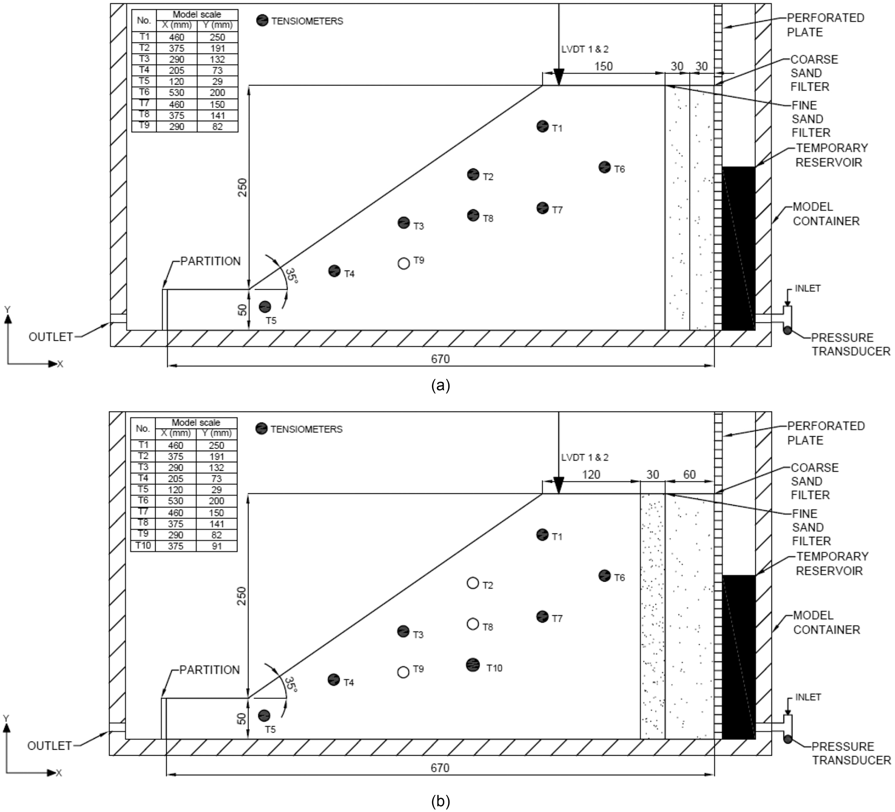
Two centrifuge tests were conducted at the Geotechnical Centrifuge Facility at the University of Pretoria, South Africa (Jacobsz et al. 2014). The model tailings dam embankments were designed and prepared using gold tailings. In the two tests, GT-1 and GT-2, where GT denotes gold tailings, the model slopes were subjected to a rising groundwater table, modelled using a viscous fluid. Schematic diagrams of the model slopes before testing are shown in Fig. 1. Vertical and horizontal offsets of the tensiometers, measured from the bottom left strongbox corner, are presented. For both tests, the model scale was and hence the design gravitational acceleration was . Appropriate scaling laws for the centrifuge tests conducted are summarized in Table 1.
| Parameter | Unit | Scale |
|---|---|---|
| Acceleration | ||
| Linear dimension | m | |
| Stress | kPa | 1 |
| Strain | — | 1 |
| Density | 1 | |
| Permeability | ||
| Viscosity | μ | 1 |
| Time | s |
Index Properties of Gold Tailings
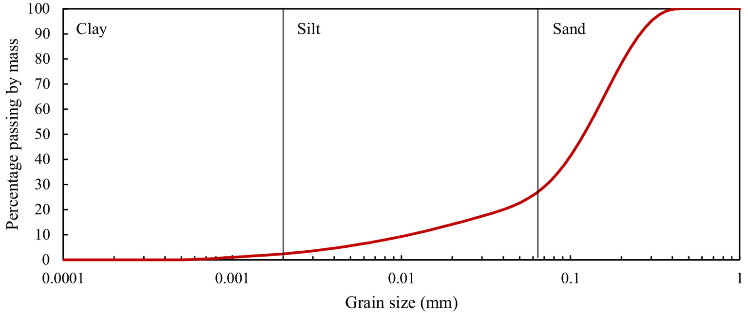
The gold tailings used in this study was obtained from a gold mine situated east of Johannesburg, South Africa. The material was collected from the daywall of the tailings dam. Based on the particle size distribution (PSD), shown in Fig. 2, the gold tailings used in this study is classified as a silty sand. The tailings has a fines content () of 26.5%, an average grain size of 120 , and a maximum particle size of 500 μm. The saturated coefficient of permeability, , was estimated using Hazen’s (1930) equation:where is the Hazen’s effective grain size (mm). The gold tailings has a specific gravity, , of 2.65. The index properties of the gold tailings are summarised in Table 2.
(1)
Model Preparation
The model slopes were constructed in a container with interior dimensions of (Fig. 1), intending to model plane-strain conditions. The container was constructed from 50 mm thick aluminum panels and was fitted with a 50 mm thick glass panel to allow observations.
Twin sand filters comprised of a coarse sand filter, followed by a fine sand filter, were placed immediately upstream of the model slopes. This was done to prevent potential internal erosion in the dam slope (Ng et al. 2022) during the fluid level rise. The filters allowed for the viscous fluid to seep slowly and evenly before reaching the tailings slope. The permeability of the coarse sand filter was on the order of and that of the fine sand filter .
The model slopes were prepared using moist tamping. This method was chosen because capillary effects between soil particles allow for the preparation of loose specimens (Castro 1969; Sladen et al. 1985; Kramer and Seed 1988; Konrad 1990; Ishihara 1993; Cai 2001). The moist tamping method also allows a contractive fabric with strain-softening tendencies, which is more susceptible to liquefaction, to be created (Chang et al. 2011). Both model slopes were formed by moist tamping the gold tailings in six 50 mm horizontal layers at an initial moisture content of 6.5%. The density was controlled by placing a predetermined amount of soil in each layer and compacting the material by hand in 50 mm layers. A temporary steel plate shutter was placed at the upstream end of the model at the boundary between the tailings and sand filters. Once a layer of tailings was compacted, the twin sand filters were placed at the upstream end of the models, also with a thickness of 50 mm each. Once six layers had been compacted, i.e., a thickness of 300 mm, the slope was cut by hand to an angle of 35° to the horizontal. The model slope in Test GT-1 was prepared at an initial void ratio, , of 0.950 and in Test GT-2 of 0.845.
Groundwater Control System
A groundwater system similar to Ng et al. (2022) was adopted and modified for this study. The system consisted of a fluid storage tank, a solenoid valve, a pressure transducer, a perforated steel plate covered by geotextile, an aluminum partition at the toe of the model slope, and an outlet. A perforated plate was installed upstream of the model slope to create a reservoir that allowed for the control of the hydraulic head upstream of the slope (Fig. 1). The perforated plate was covered with geotextile to prevent sand from filling the reservoir. A fluid storage tank, holding the viscous fluid, was mounted near the centrifuge rotation axis and was connected to the reservoir upstream of the slope via 8 mm plastic tubing. The fluid level in the reservoir was controlled using a solenoid valve. A pressure transducer installed at the inlet of the model container monitored the hydraulic head in the reservoir. The fluid level at the downstream end of the model slope was controlled using an aluminum partition plate with a height equal to that of the toe of the slope. As the fluid seeped through the model slope, the fluid level rose until it overflowed the partition, thus maintaining a downstream level constantly level with the toe, preventing inundation of the lower parts of the slope.
Viscous Fluid
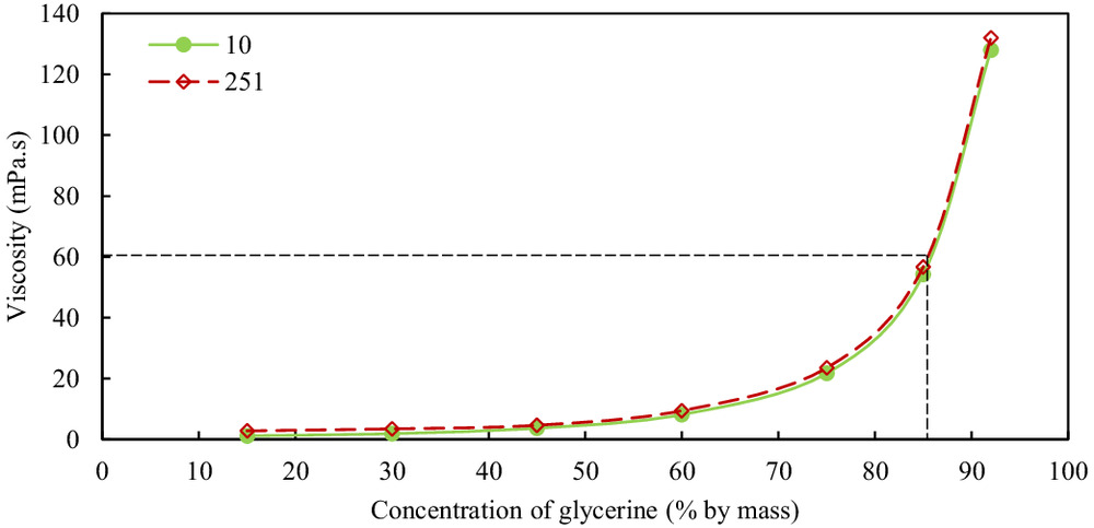
The intention with the centrifuge models was to investigate flowslide behavior during slope instability. It was therefore desirable to create instability-type events in the centrifuge. In order to successfully model the flowslide behavior of the slope and the subsequent dissipation of excess pore pressures, it was necessary to increase the viscosity of the pore fluid linearly with the scale factor (Askarinejad et al. 2014; Take et al. 2004; Zhang and Askarinejad 2021). The viscosity therefore had to be 60 times that of water to appropriately scale the dissipation of excess pore pressures. For both centrifuge tests, a mixture of glycerine and water was used. To determine the concentration glycerine required, a series of glycerine-water mixtures were prepared with 15%, 30%, 45%, 75%, 85%, and 92% glycerine. The viscosity of each mixture was measured at 25°C using a rheometer. In addition, the viscosities of the mixtures were measured at varying shear strain rates (). Fig. 3 shows the viscosity of the mixtures at 25°C and shear strain rates of 10 and . From the viscosity relationship shown in Fig. 3, a glycerine-water mixture with 86% glycerine and 14% water was chosen to obtain a fluid with a viscosity 60 times higher than water. The temperature within the centrifuge facility was set at 25°C using a dedicated ventilation system, which allowed for the viscosity of the fluid to remain unchanged. More details about the selection of a viscous fluid can be found in Crous et al. (2022).
Instrumentation
To monitor the response of the pore fluid pressure, tensiometers developed at the University of Pretoria were constructed (Jacobsz 2018). The tensiometers are able to measure both positive and negative pore fluid pressures. The tensiometers were installed at various locations throughout the model slopes to give a comprehensive view of the slope response throughout the tests (Fig. 1). Some of the tensiometers dried prior to the centrifuge tests, so that some readings could not be used. The tensiometers that dried are indicated by the white circles in Fig. 1.
Two linear variable differential transformers (LVDTs) were installed at the crests of the model slopes to monitor crest settlement during the tests. To capture the rapid slope failures during the centrifuge tests, a continuous recording of the slope responses was required. Two video cameras were used to monitor and record the response of the model slopes during the centrifuge tests. One camera was placed in front of the window and a second camera was installed to give an oblique view of the slope face. Both video cameras had a display resolution of pixels with a frame rate of 30 frames per second.
Centrifuge Modelling Test Procedure
Tests GT-1 and GT-2 followed the same general procedure. The slight differences between the two tests are discussed in detail subsequently. Both model slopes were accelerated to 60 g. As the model slopes were prepared at a loose state, the slopes experienced settlement during acceleration. Once 60 g was achieved, settlement was monitored until settlement stopped, upon which the wetting process was initiated. The solenoid valve was opened, which allowed the upstream reservoir to fill and the fluid to seep into the model slopes. Once the fluid level in the reservoir was close to the crest of the slopes, the solenoid valve was closed. The hydraulic head in the reservoir was continuously monitored and the solenoid valve was opened and closed accordingly to maintain a constant fluid level in the reservoir. The fluid seeped from the reservoir in the downstream direction, progressively raising the fluid level. The wetting process continued until the model slopes experienced a flow failure. Once the failure events had occurred, the centrifuge was stopped. The pore fluid pressures and crest settlements were monitored throughout the tests. For Test GT-1, the instrumentation sampling rate was 1 Hz. In retrospect, this was somewhat low, therefore the sampling rate was increased to 10 Hz for Test GT-2.
Numerical Analysis
In addition to the centrifuge tests, a numerical back-analysis of Test GT-2 was conducted using the finite element program PLAXIS 2D, in order to verify the postulated trigger and failure mechanism observed during the test. The tailings dam slope was modelled used the NorSand model (Jefferies 1993). The current implementation of NorSand in PLAXIS 2D does not contain an internal cap, which controls the maximum dilatancy of the soil by limiting the yield surface hardness (Jefferies 1997). Thus, it was necessary to investigate the simulated soil behavior during an unloading (CSD) stress path, which was done using element-scale unloading (CSD) stress path simulations.
Finite Element Mesh and Boundary Conditions
A bi-axisymmetric model triaxial specimen was used to investigate the simulated soil behavior during a CSD stress path. Fig. 4(a) shows the two-dimensional mesh, dimensions, and boundary conditions used for the element-scale numerical CSD stress path simulations. Fifteen noded triangular elements were used for the model. The dimensions of the model were . The bottom and left boundaries that were normally fixed at the top and right boundaries were set as free. Line loads were applied to the top and right boundaries in order to control the confining and shear stress.
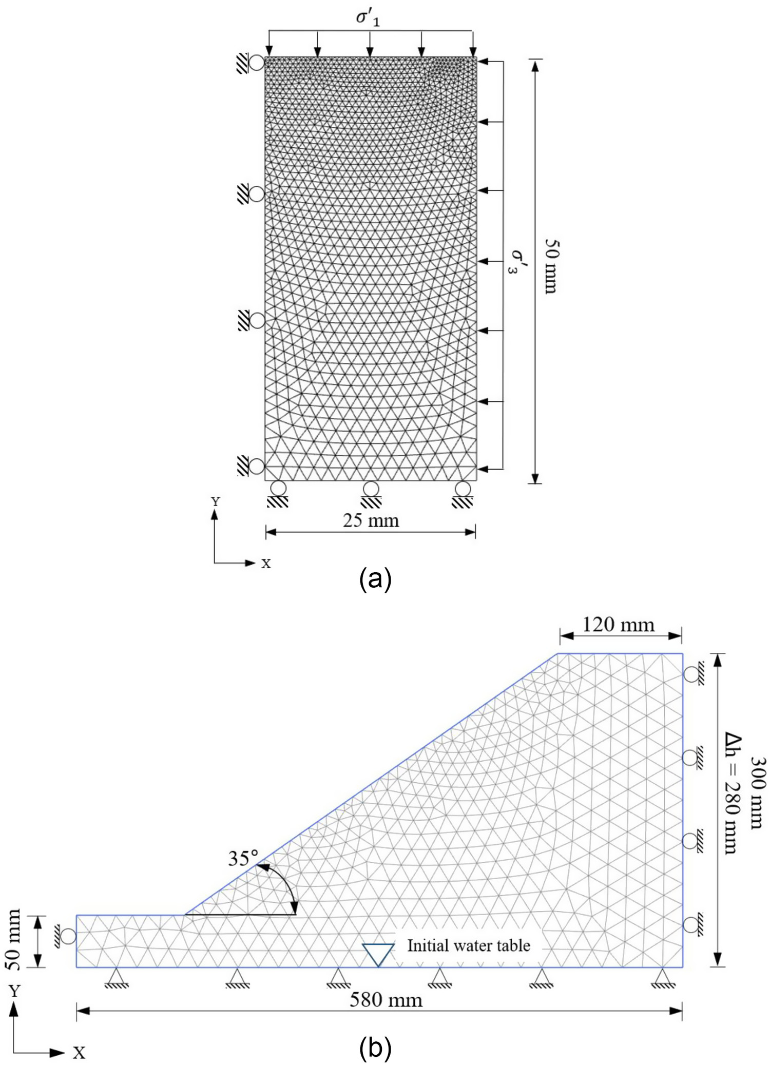
Fig. 4(b) shows the two-dimensional mesh, dimensions, and boundary conditions used for the numerical back-analysis of Test GT-2. Fifteen noded triangular elements were used for this model. The dimensions are at the model scale. The boundary conditions and dimensions were chosen to be as consistent with the centrifuge tests. The sand filters upstream of the model were not considered in the numerical analysis. The slope angle was set at 35° to replicate the initial geometry of the model slope. The initial water level was set at the bottom boundary of the model. The surfaces of the slope crest, slope face, and at the toe of the slope were set as seepage boundaries. The bottom and downstream vertical boundaries were set as impervious, except the groundwater flow boundary at the downstream end, which was set as open to model the boundary conditions of the centrifuge test.
Constitutive Model and Model Parameters
The critical state framework provides a strong framework to formulate constitutive models that can adequately predict soil behavior associated with static liquefaction (Jefferies and Been 2016). Jefferies (1993) introduced such a constitutive model with NorSand. Despite containing “sand” in the name, NorSand is applicable to all soils where contact forces, instead of bonding, control particle to particle interactions (Shuttle and Jefferies 2010). The NorSand model is state dependent, and the response of a soil can be predicted considering the initial void ratio. The NorSand model parameters (, , ,, , , , , , and ) were determined for the gold tailings from a series of triaxial tests.
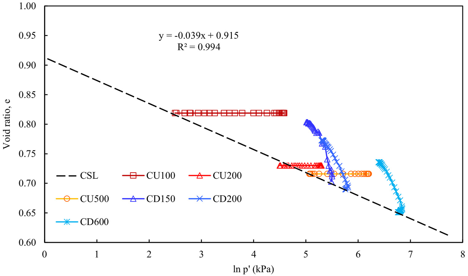
The critical state line (CSL) in the state diagram ( space) was determined from a series of drained and undrained triaxial tests (Fig. 5). CU represents isotropically consolidated undrained triaxial compression tests and the number following denotes the initial confining pressure. CD represents isotropically consolidated drained triaxial tests and the number following denotes the initial confining pressure. The CSL in the state diagram can be expressed aswhere = void ratio of the CSL at ; and = slope of CSL in the state diagram. For the gold tailings used in this study, and provided the best fit.
(2)
The volumetric coupling coefficient, , does not vary significantly and is often assumed to be 0.3 for simplicity (Shuttle and Jefferies 2010; Jefferies and Been 2016). To calibrate the state dilatancy parameter, , drained tests need to be conducted on dense specimens to get a dilative response. Despite preparing some triaxial specimens as dense as possible, it was not possible to achieve a dilative response using moist tamping. Thus, could not be calibrated for the gold tailings used and it was assumed to be 3.2, following Reid and Smith (2021).
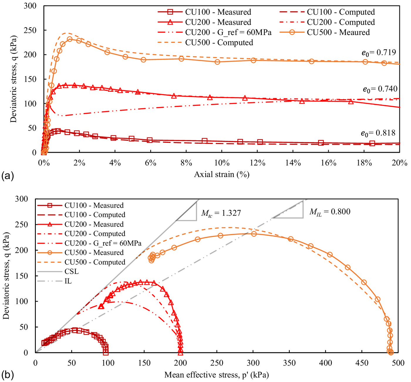
Fig. 6 shows the shear behavior of the gold tailings for isotropically consolidated undrained triaxial compression tests, along with the calibrated NorSand model predictions. Figs. 6(a and b) compare the measured and predicted stress-strain behavior and effective stress paths for the undrained triaxial tests, respectively. As bender elements were not available for the triaxial tests, the elastic shear modulus, , and the elastic exponent, , were adopted, following Theron et al. (2004), as 60 MPa and 0.65, respectively. However, as noted by Shuttle and Jefferies (2016) and Reid and Smith (2021), there is an issue with the implementation of the elastic bulk modulus, , in NorSand when calibrating the model for silts. NorSand estimates from the geophysically measured usingwhich requires a constant and representative Poisson’s ratio, . As discussed by Shuttle and Jefferies (2016), when a geophysically based is used, the predicted response of the NorSand model produces a too-stiff initial response, which subsequently develops into a sharp transient loss of strength, followed by strong dilation to the correct critical state. Thus, the predicted value does not compare with the measured. This behavior is evident when comparing the measured and predicted values for specimen CU200 (Fig. 6). To circumvent this issue, Shuttle and Jefferies (2016) and Reid and Smith (2021) recommend that the elasticity values be reduced by a factor of up to four for some tailings when calibrating the NorSand model. Thus, a of 15 MPa was adopted for this study to produce the best fit between the measured and predicted values. Table 3 summarizes the model parameters used.
(3)
| Parameter | Value and unit |
|---|---|
| Void ratio of the CSL at , | 0.915 |
| Slope of the CSL, | 0.039 |
| Critical state ratio, | 1.327 |
| Reference elastic shear modulus, a | 15 MPa |
| Elastic exponent, a | 0.65a |
| Poisson’s ratio, b | 0.3 |
| Volumetric coupling coefficient, b | 0.3 |
| State-dilatancy parameter, c | 3.2 |
| Plastic hardening modulus (base value), | 122.2 |
| Plastic hardening modulus, | 914.0 |
From Fig. 6(a), it is evident that the predicted stress-strain behavior of the calibrated NorSand model is in good agreement with the measured values for loose gold tailings. It can be seen that the NorSand model can also adequately predict the effective stress paths of undrained triaxial tests [Fig. 6(b)]. As the mean effective stress, , decreases, the deviatoric stress, , increases until a peak is reached. After the peak, the deviatoric stress starts to decrease along with the mean effective stress. An important characteristic of the NorSand model is that it is able to capture the strain-softening behaviour of loose gold tailings during undrained shearing. After reaching a peak deviatoric stress, the shear strength decreases where large strains develop.
Also shown in Fig. 6(b) is the CSL determined from a series of drained and undrained triaxial tests. The slope of the CSL under triaxial compression, , is 1.327, which corresponds to a critical state friction angle, , of 33°. It should be noted that the numerical model used in this study is under plane strain conditions. While a constant value of can be determined for triaxial compression conditions, as noted by Bishop (1966), the intermediate principal stress has an effect on the critical friction ratio, . The stress state in plane strain varies from one plane strain state to another, because the stress state develops to accommodate the imposed strain condition. The stress state is often denoted by the Lode angle, , which is a stress invariant that ranges from in triaxial compression to in triaxial extension, with all other stress states lying between these limits (Jefferies and Been 2016). Thus, the critical state friction ratio as a function of Lode angle, , is used as a general concept for the critical state friction ratio, where is used as an input parameter into NorSand, to scale (Woudstra 2021).
Based on the definition by Lade (1992), instability lines (ILs) can be found by connecting the peaks of the undrained stress paths within the origin of the plane. The average instability line (IL) for the gold tailings used in this study is shown in Fig. 6(b). As shown by Yang (2002), the slope of the IL, , is state dependent (i.e., the slope varies with the state parameter). Thus, the throughout the model slopes will vary. However, the average for the three undrained triaxial tests conducted shown is 0.800. This corresponds to an average mobilised friction angle at the peak, , of 21° applicable to undrained conditions. In order to induce instability, or trigger static liquefaction, the slope needs to be in a loose, saturated state and the soil must have a contractive tendency, which will cause strain-softening during undrained shearing (Take and Beddoe 2014). In addition, the minimum slope angle required for a slope to become unstable under undrained conditions, , can be determined using the following equation (Lade and Yamamuro 2011):where = the friction angle of the soil. For the gold tailings used, this translates to a minimum slope angle of 16.7°.
(4)
The implementation of NorSand in PLAXIS 2D requires that a uniform state parameter, , be assigned to the material. To mitigate this issue, multiple layers with different values can be created and assigned to the model. However, for simplicity, a of 0.122 was adopted for the back-analysis of Test GT-2, which corresponds to the state parameter at an average depth of 125 mm in the model slope. It should be noted that consolidation will take place in situ. This can lead to shear densification within the slope. Thus, in order to study the impact of shear densification on the instability behavior of the numerical model, a parametric study was conducted. Two additional analyses were conducted using the same calibrated model and numerical procedure, but with values of 0.03 and 0.06. The used for the CSD stress path simulations were varied between –0.10 and 0.20, to determine whether a trend between the modified state parameter (the difference between the void ratio at the onset of instability and at the critical state, ) and can be established [after Chu et al. (2003)].
The unsaturated and saturated unit weights were set as 15.0 and , respectively. These values correspond to the respective unit weights of the model slope in Test GT-2. The saturated permeability of the gold tailings was set as (i.e., 60 times less than that of the tailings) for all analyses to satisfy the scaling law for seepage flow due to the viscous fluid used in the test. The initial pore fluid pressure measured by the tensiometers in the centrifuge tests was approximately . Thus, a suction of 15 kPa was applied to the model slope in the numerical analysis. For the initial stages of the numerical analyses, modelling the acceleration of the centrifuge, a Mohr-Coulomb model was used with a gold tailings friction angle, , of 33°, as well as a of 0.3.
Numerical Modelling Procedure
The numerical simulation of a CSD test simulates the stress path that soil elements followed during, and the numerical back-analysis of, Test GT-2. Three stages were used to simulate the CSD stress path. As will be discussed later, the initial stages of the back-analysis of Test GT-2 required the use of the Mohr-Coulomb model to obtain convergence. Thus, for Stage 1 of the CSD test simulation, initial conditions were set by applying gravity loading to the model using the Mohr-Coulomb model. During Stage 2, the model was anisotropically sheared under drained conditions using the Mohr-Coulomb model by linearly increasing and by 120 and 45 kPa, respectively. This resulted in a stress path similar to what a soil element experiences during centrifugal acceleration (to be discussed). After this stage, the material model was substituted for the calibrated NorSand model for Stage 3. During Stage 3, the model was subjected to a CSD stress path by linearly reducing and at the same rate, keeping the deviatoric stress constant whilst reducing the mean effective stress, until collapse was triggered.
Three stages were used for the numerical back-analysis of Test GT-2. During Stage 1, initial conditions were set by applying gravity loading to the model using the Mohr-Coulomb model. During Stage 2, the gravitational acceleration of the model slope was simulated by increasing the gravity level from 1 g to 60 g while still using the Mohr-Coulomb model in order to obtain convergence. The gravity level was progressively raised in order to mimic the centrifuge modelling process. After increasing the gravity level to 60 g, the material model was substituted for the calibrated NorSand model for Stage 3. During Stage 3, a hydraulic head of 280 mm was applied at the upstream side of the model [Fig. 4(b)] to allow the water to seep into the slope, modelled using a fully coupled transient flow-deformation analysis until slope failure was triggered. No additional stages were required, as the model predicted the drained instability of the slope during Stage 3. Stress points at the locations of T1, T3-T7, and T10 [Fig. 1(b)] were monitored during the numerical back-analysis, allowing for comparison with the measured pore fluid pressure response during Test GT-2.
Retrogressive Flowslide Failure: GT-1
In this section, the measured results for Test GT-1 are discussed and compared. Although the model slope in Test GT-1 was constructed at an angle of 35°, steeper than the of 33° for the gold tailings used in this study, the slope settled to an angle of 32° before failure. In addition, the slope was steeper than the minimum slope angle required for the slope to become unstable under undrained conditions (16.7°). During Test GT-1 problems were encountered with the solenoid valve controlling the hydraulic head in the reservoir. At the initial stages of the test the solenoid valve would not close, which caused the reservoir to overfill, resulting in the slope overtopping on the side of the model slope against the strongbox window and the centrifuge was stopped. The overtopping only caused minor surface erosion of the model slope on the side of the window, which was deemed to be superficial, leaving the slope structurally intact. Further problems with the solenoid valve caused the centrifuge to be stopped twice more before problems were rectified.
Slope Response during Rise of Water Table in Test GT-1
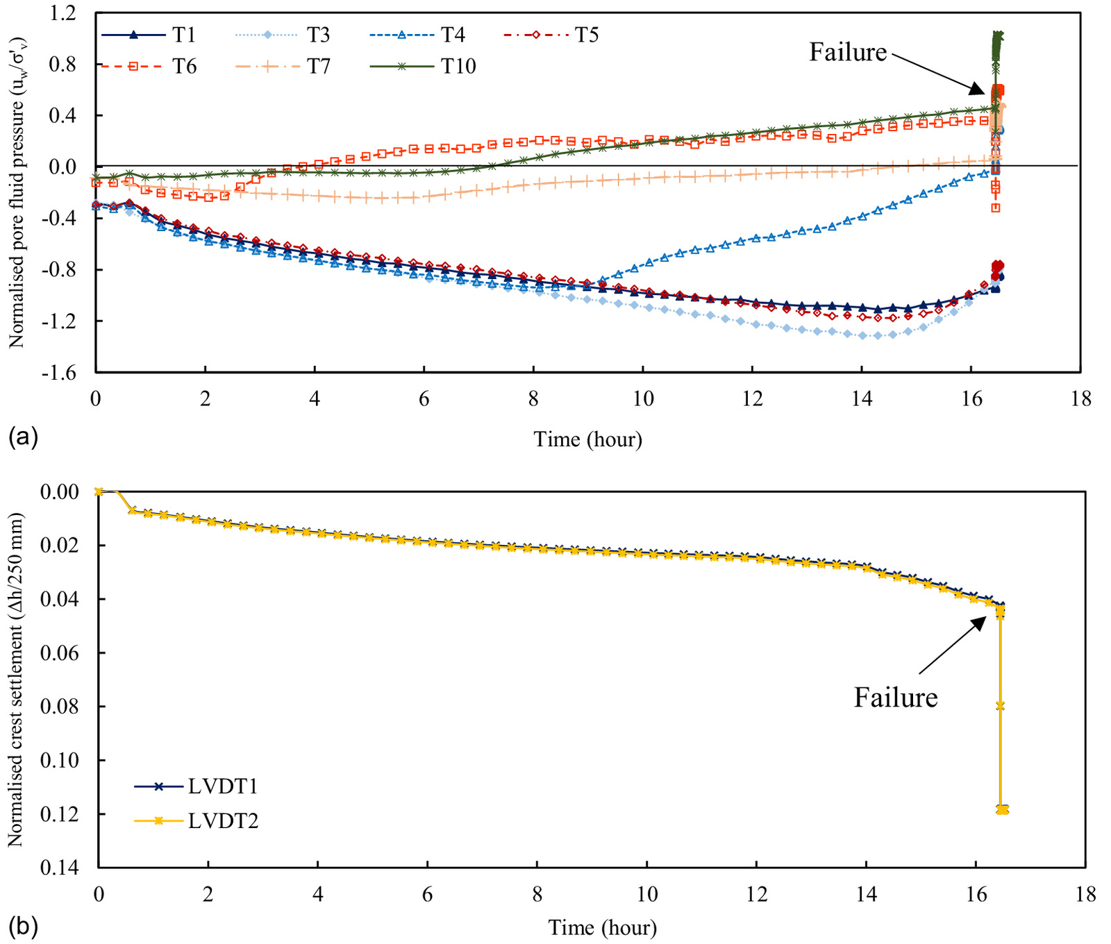
Figs. 7(a and b) show the measured pore fluid pressures normalized by the initial vertical effective stress, and the measured crest settlements normalized by the initial slope height during Test GT-1. Nine tensiometers (T1-T9) were installed in the slope [Fig. 1(a)], but T9 cavitated prior to the test. All functioning tensiometers measured a pore fluid pressure between and at the start of the test. When the slope was at the design centrifugal acceleration, the pore fluid pressures started to gradually decrease [Fig. 7(a)] due to the downward migration of moisture under high acceleration, as was also observed by Poulose et al. (2000). This trend was temporarily interrupted by the stoppages. As the water table neared the tensiometers, the pore fluid pressure started to increase. Once the phreatic surface reached the location of a tensiometer, the pore fluid pressure increased further, measuring positive pore pressures. The measured pore fluid pressure at T5, which was installed at the toe of the slope [Fig. 1(a)], plateaued after roughly 7 h [Fig. 7(a)] as the soil above T5 became completely saturated. Thus, as the water table continued to rise throughout the slope upstream of the toe, the head at T5 stayed constant.
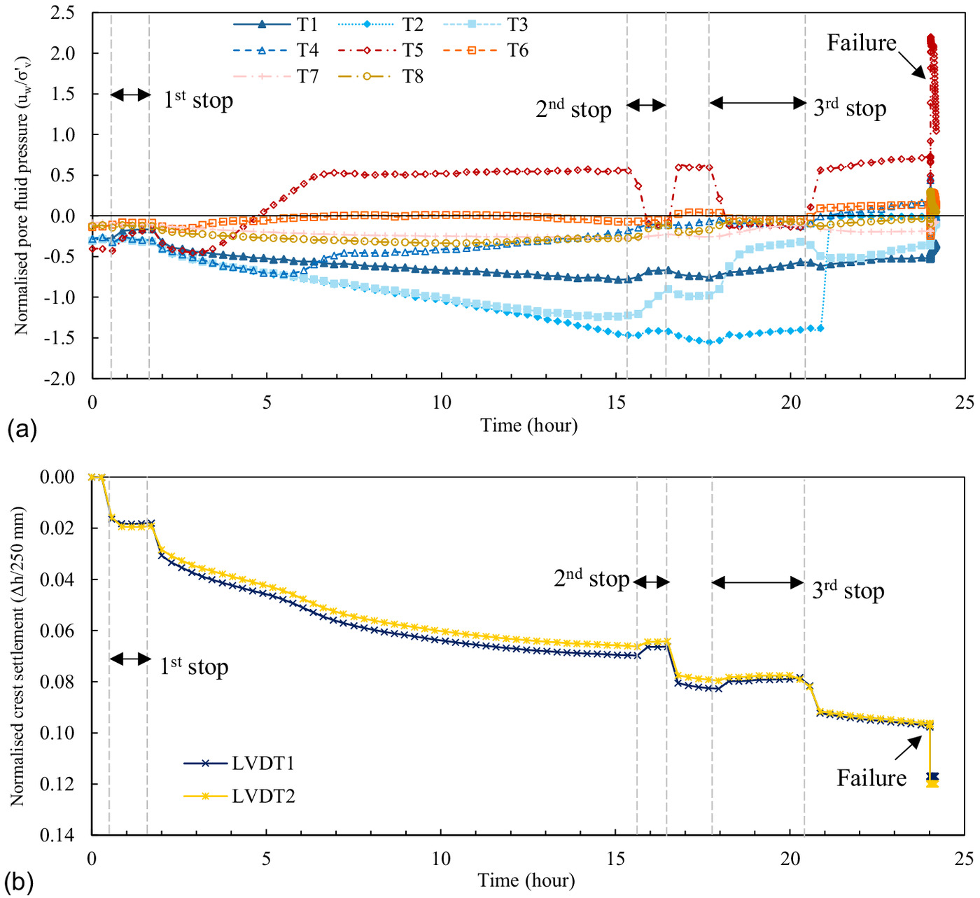
As seen in Fig. 7(b), once the viscous fluid started to seep into the slope, rapid settlement was induced at the crest of the slope, indicating volumetric reduction of the slope due to the loss of matric suction as the slope was wetted (Jennings and Burland 1962; Chang et al. 1981; Sladen et al. 1985; Ng et al. 1998; Vaid and Sivathayalan 2000). After 24 h of wetting, the model slope experienced a flow failure. At this point, rapid fluctuations in the pore pressures were measured, along with sudden crest settlements. After the failure of the slope, excess pore pressures dissipated rapidly. The plateaus in the LVDT readings denote the end of travel.
Observed Trigger and Failure Mechanism of Slope in Test GT-1
The images of the failure sequence of the slope in Test GT-1 (Fig. 8) were captured by the video camera, looking downward onto the slope face. The camera recording the side view malfunctioned during the test.
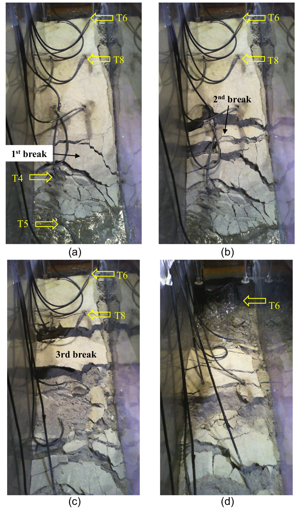
The failure of the model slope was a retrogressive failure that initiated at the toe and progressed upstream until a flow slide failure was triggered. For discussion purposes, the reference time in this section is taken as the time when the first break in the slope occurred [i.e., Fig. 8(a)]. The failure process of the model slope can be divided into four main stages.
Due to large seepage forces, sloughing occurred at the toe and large tensile cracks formed above the toe of the slope before the failure event. A large soil mass near the toe broke away from the slope where the cracks formed, initiating the failure process. This break is defined as Stage 1. The initial break was slow moving, having an estimated velocity of based on the time of sliding (1.9 s). This break resulted in a loss of confinement at the toe of the slope. This loss of confinement resulted in the soil upstream in the model slope losing confining stress so that it was no longer supported by the material at the toe. This triggered a second soil mass to break away from the slope, defined as Stage 2 [Fig. 8(b)]. This break was more rapid than the initial break, with an estimated peak velocity of . During Stages 1 and 2 no deformation was induced in the upstream section of the slope. However, Stage 3 was initiated after a more rapid third break that occurred 6.5 s after the initiation of the first break [Fig. 8(c)]. The third break had an estimated peak velocity of . Just 0.9 s after the third break occurred, the remainder of the slope rapidly collapsed, which resulted in a flowslide failure [Stage 4, Fig. 8(d)]. This final collapse had an estimated peak velocity of . Kennedy et al. (2020) observed a similar retrogressive landslide failure in a sensitive clay model slope. It is hypothesized that the Merriespruit tailings dam experienced a similar retrogressive failure, causing static liquefaction of the tailings and a large flow failure (Wagener et al. 1998; Fourie et al. 2001; Mànica et al. 2022). Cuomo et al. (2019) simulated a flume test that experienced a similar retrogressive slope failure that transitioned into a liquefaction failure, using the material point method.
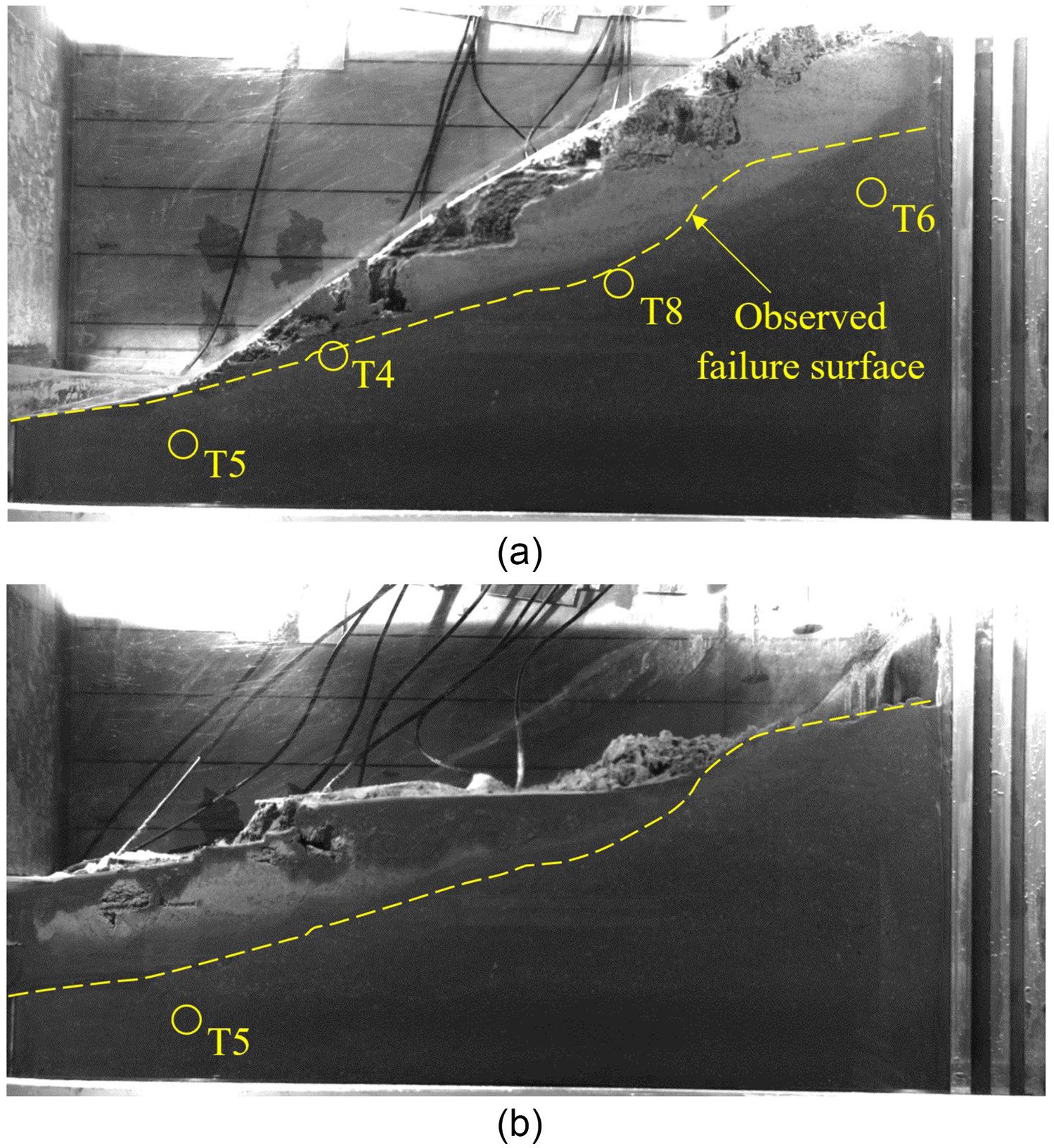
Side views of the slope before and after the failure are shown in Figs. 9(a and b), respectively. The observed failure surface cutting through the locations of T4, T5, T6, and T8 is indicated. Only these tensiometers are indicated as only these sensors measured significant pore pressure fluctuations during the failure event (discussed subsequently). Only T5 is indicated in Fig. 9(b), as it was difficult to estimate the post failure locations of T4, T6, and T8.
Measured Excess Pore Pressures and Crest Settlement during Slope Failure in Test GT-1
Fig. 10 shows the measured excess pore pressure ratios, , and normalised crest settlement immediately before, during, and after the failure of the model slope in Test GT-1, where is the excess pore pressure and is the initial vertical effective stress estimated from the slope profile before failure [Fig. 9(a)] at the location of each tensiometer [Fig. 1(a)]. Time zero in Fig. 10 is set at five seconds before the initiation of the failure event. T1, T2, T3, and T7 all measured negative pore pressures at the time of failure [Fig. 7(a)], indicating that the tensiometers were located in the unsaturated soil of the model slope. These tensiometers did not measure any significant changes in pore pressure during the failure event. Thus, only the measured responses of T4, T5, T6, and T8 are presented in Fig. 10.
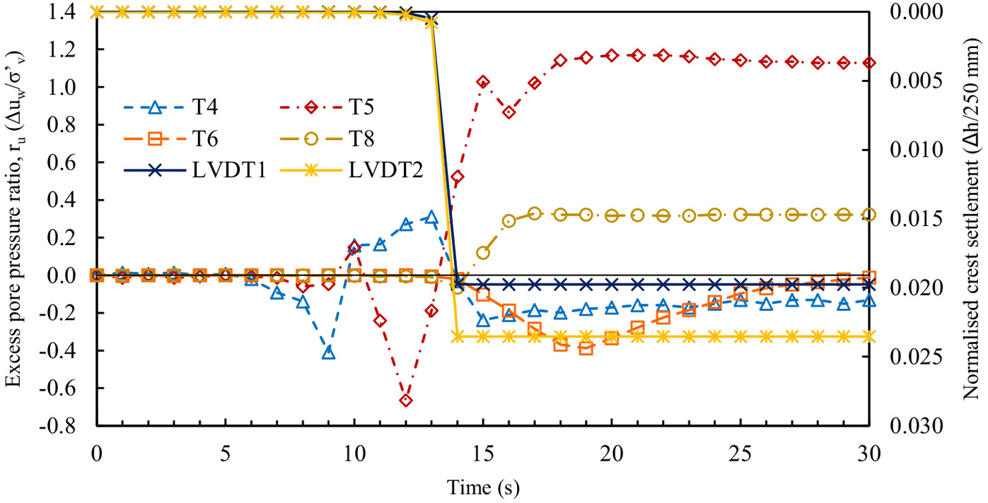
As shown in Fig. 8(a), the first break occurred at the toe of the slope, where T4 and T5 were located. This is reflected by the measured changes in pore fluid pressure (Fig. 10). Only T4 and T5 initially measured a response, whilst T6 and T8 did not measure any changes. In addition, at the moment T4 and T5 measured a response, LVDT1 and LVDT2 had not yet measured any crest settlements, indicating that the soil near the crest did not experience any deformation, yet both T4 and T5 initially measured a decrease in pore fluid pressure (i.e., negative excess pore pressure). It is believed that the dilatant response was caused by tension in the tensiometer cables. As the slope started to move, the tensiometer cables would have been pulled, causing some dilation around the tensiometers, resulting in negative excess pore pressures. However, after the slight drop in pore pressure, both tensiometers measured positive excess pore fluid pressures. This fluctuation in the pore fluid pressure confirmed that the soil sheared under at least partially undrained conditions. The positive excess pore fluid pressures indicate the soil’s contractive tendency. T4 measured a peak excess pore fluid pressure of 13.2 kPa and T5 measured a peak of 49.8 kPa . T4 measured a . However, and unlike level ground, full liquefaction is not a prerequisite for slope failure. In contrast, T5 measured an . After this point, the excess pore pressure dropped slightly before increasing again, this time reaching a peak .
An aspect to consider is the rate of shearing. Looking at Fig. 10, the pore pressures increased by 76 kPa () at T5 within a span of three seconds. This indicates that the rate of shearing in the region of T5 was rapid. This rapid shearing resulted in the generation of significant positive excess pore pressures, and prevented the dissipation of the excess pore pressures. This led to a degree of localized liquefaction around the toe of the slope. Once the soil in the region experienced a degree of localized liquefaction, the tailings could not support the tailings upstream of the toe. As a result, the tailings upstream of the toe experienced a loss of confinement and a loss of support, which triggered the retrogressive failure (Fig. 8).
As noted previously, T6 and T8 initially did not measure a response at the initiation of the slope failure. However, the retrogressive failure of the slope (Fig. 8) was triggered due to a degree of localized liquefaction in the region of T5, and T6 and T8 only measured a response once the failure had progressed upstream and reached the crest of the slope (Fig. 10). At the time that T6 and T8 measured a response, both LVDT1 and LVDT2 measured changes in crest settlement as well. This indicates that, as soon as the crest started to deform, the tailings at T6 and T8 started to shear. Like T4 and T5, T8 initially measured negative excess pore pressures, which was soon followed by positive excess pore pressures, indicating the tailings had a contractive tendency. In contrast, T6 only measured negative excess pore pressures before returning to the original value. T6 measured a minimum excess pore pressure of and T8 measured a peak excess pore pressure of 28.0 kPa . The negative measured by T6 could be due to the tensiometer being pulled from the soil during the failure event.
The measured positive excess pore pressures, specifically around the toe region, led to a significant reduction in effective stress, and thus in the shear strength of the slope. This reduction in shear strength due to the rapid undrained shearing triggered a degree of localized liquefaction at the toe of the slope. Eckersley (1990), Wang and Sassa (2000), Moriwaki et al. (2004), Take and Beddoe (2014), and Ng et al. (2022) also reported positive excess pore pressures during slope failures in flume and centrifuge tests. It was concluded that the excess pore pressures were generated due to the contractive tendency of the loose soils used in the tests. Furthermore, the magnitude of excess pore pressures generated depended on the rate of deformation as well as the soil state (i.e., stress state and void ratio). Based on the observed failure mechanism (Fig. 8), the rapid rate of shearing, the large measured positive excess pore pressure ratios at the toe of the slope (Fig. 10), and the long flow out distance of the failure, it can be concluded that the retrogressive failure was triggered by drained instability at the toe of the slope, which triggered the localized liquefaction at the toe.
Slide-to-Flow Failure: GT-2
This section discusses and compares the measured and computed results for Test GT-2. The model slope in Test GT-2 was constructed at an angle of 35°, which is steeper than the of 33° for the gold tailings used in this study. However, the slope settled to an angle of 33° prior to the failure of the slope. Although this was equal to the , the failure of the slope initiated in the unsaturated zone of the slope. Thus, the failure event was not triggered by a loss in matric suction. The video record of the failure event is from the side. Furthermore, as it was hypothesized that some excess pore pressures dissipated during the failure event between data sampling in Test GT-1, the data sampling rate was increased to 10 Hz for Test GT-2.
Slope Response during Rise of Water Table in Test GT-2
Figs. 11(a and b) respectively show the measured pore fluid pressures normalized by the initial vertical effective stress and crest settlements normalized with the initial slope height during the rise of the water table in Test GT-2. Ten tensiometers (T1–T10) were installed in the slope [Fig. 1(b)], but T2, T8, and T9 dried prior to the test and their readings are therefore not shown. The initial pore pressure response during Test GT-2 was similar to that of Test GT-1. However, unlike the observations in Test GT-1, the measured pore fluid pressure continued to decrease around the toe of the slope (i.e., T5). In contrast to Test GT-1, the centrifuge was not stopped during this test. This resulted in the fluid level being raised more rapidly than in Test GT-1. It is thus possible that the degree of saturation of the soil in the toe region was low, resulting in negative pore pressures being measured in the toe region. Owing to the lower degree of saturation in the toe region, it was more difficult to induce localized liquefaction in the toe region. It is also possible that T5 dried out before the phreatic surface reached the tensiometer, which would result in a slow response.
As seen in Fig. 11(b), the crest of the slope settled gradually as the viscous fluid seeped into the slope, which indicates that volume reduction occurred due to a loss of matric suction. The rate of settlement accelerated when the pore pressures near the base of the slope began to rise (T1, T3, and T5). However, the initial rate of settlement was lower than that in Test GT-1, due to the model slope in Test GT-2 being denser that the slope in Test GT-1. The rate of settlement started to reduce throughout the test but increased at around 14 h into the test. At this point cracks started to form in the crest of the slope, visible on the side view (discussed subsequently). After 16.4 h of wetting, the model experienced a sudden slide failure, accompanied by sudden pore pressure fluctuations [Fig. 11(a)] and crest settlement [Fig. 11(b)]. However, the trigger and failure mechanism was different than Test GT-1 (discussed subsequently). The end of the LVDT measurements denote the end of travel.
Observed Trigger and Failure Mechanism of Slope in Test GT-2
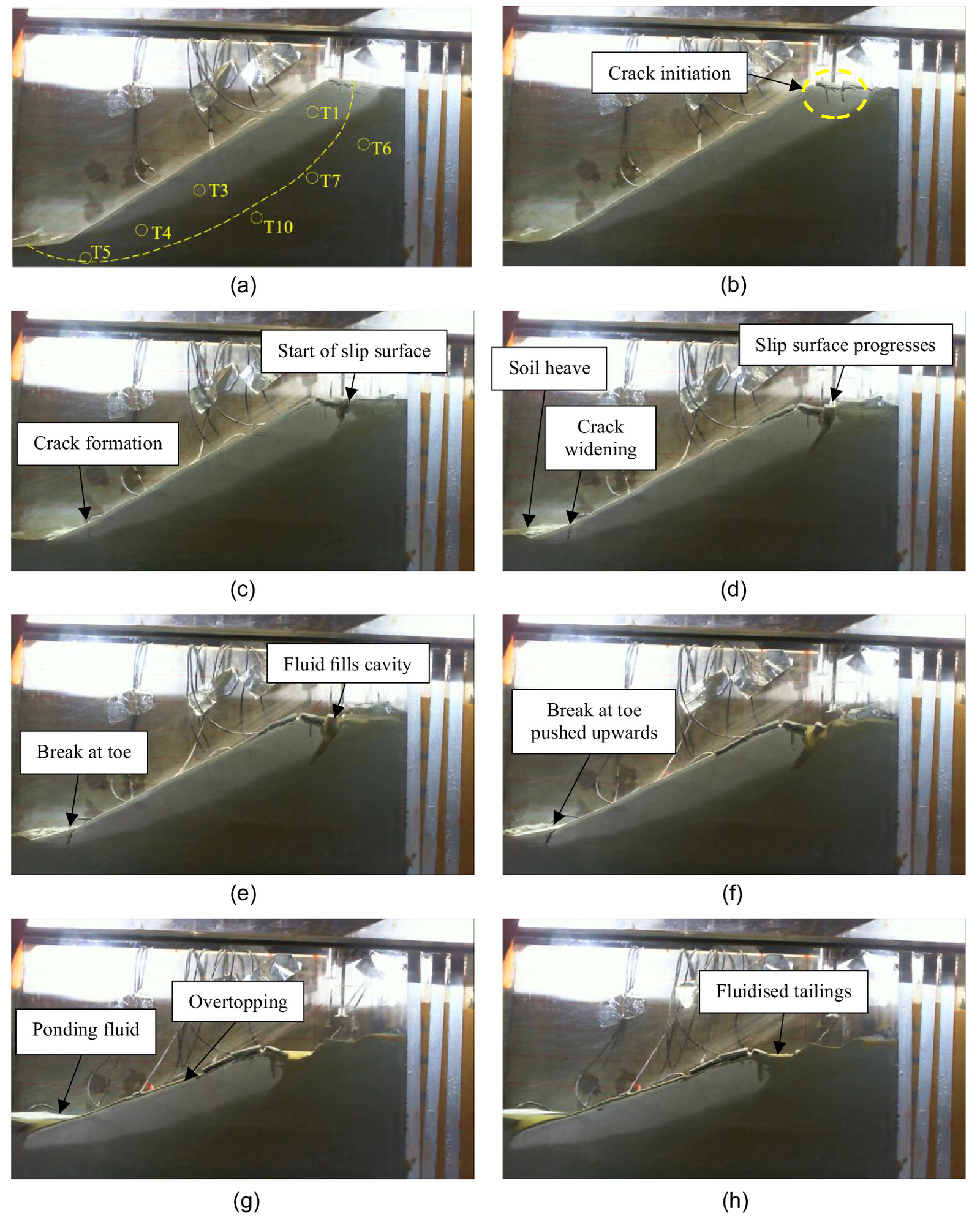
Images of the slope failure sequence in Test GT-2 as captured by the video camera from the side are presented in Fig. 12. For ease of interpretation, the reference time is set at the time of initiation of the failure event. Fig. 12(a) shows the slope profile and the location of the tensiometers prior to the failure, as well as the observed failure surface. Fig. 12(b) shows the initiation of two tension cracks that formed beneath the crest of the slope, indicating the start of slope failure. At 0.95 s, the cracks had propagated downwards and the crack furthest upstream started to transition into a slip surface [Fig. 12(c)]. Furthermore, a crack had formed at the toe of the slope. At 1.11 s, the slip surface had progressed further downwards and the crack at the toe started to widen [Fig. 12(d)]. The soil mass above the slip surface started to move downstream, causing heave at the toe. At 1.29 s the crack at the crest widened [Fig. 12(e)]. The viscous fluid started to flow into the crack, further destabilizing the sliding soil mass. At 1.68 s the soil at the toe of the slope broke away from the larger sliding soil mass [Fig. 12(f)]. The heaved soil at the toe of the slope was pushed downstream by the larger sliding soil mass. At 5.85 s the fluid that had filled the crack at the crest started to overtop the slope and flowed downstream along the slope surface, ponding at the toe [Fig. 12(g)]. At 9.95 s the sliding soil mass had settled at the downstream side of the model container [Fig. 12(h)]. Some of the tailings that were located upstream of the crest fluidized and settled in the cavity at the upstream end of the slope. The estimated peak velocity of the failure was approximately , which is significantly slower than the peak velocity during the failure in Test GT-1.
Measured Excess Pore Pressures and Crest Settlements during Failure of Slope in Test GT-2
The failure observed in Test GT-2 is different from the observed failure in Test GT-1. The failure in Test GT-1 initiated at the toe of the slope and progressed upstream, which was confirmed by the delayed response of the instruments in the slope (Fig. 10). In Test GT-2 the model slope experienced a slip failure triggered by drained instability due to the rising fluid level, and the soil mass failed as one intact mass. The failure observed was similar to the slide-to-flow transformation described by Bolton et al. (2003) and Take et al. (2004). A drained slip failure was triggered by rising pore pressure. The increasing pore pressure results in a CSD stress path, where the mean effective stress is slowly reduced whilst the deviatoric stress is kept constant. As pore pressure increased in the slope, the safety factor against slope failure reduced towards unity, by which time a sudden slope failure occurred, providing little prior warning. The slip failure triggered at least partially undrained shearing within the slope, which generated positive excess pore pressures. The geometry of the slip failure and the slow moving soil mass then transitioned into a more rapid flowslide failure. However, the flowslide failure was still slower than the observed failure in Test GT-1.
Fig. 13 shows the and normalised crest settlements immediately before, during, and after the slope failure in Test GT-2. The vertical effective stress, , was estimated from the slope profile before failure [Fig. 12(a)] and the location of each tensiometer [Fig. 1(b)]. Time zero in Fig. 13 was set as five seconds before the initiation of the failure event. T2, T8, and T9 dried out before the failure event and T1, T3, and T5 measured negative pore pressures at the time of failure [Fig. 11(a)]. Thus, only the measured responses from T4, T6, T7, and T10 are presented in Fig. 13.
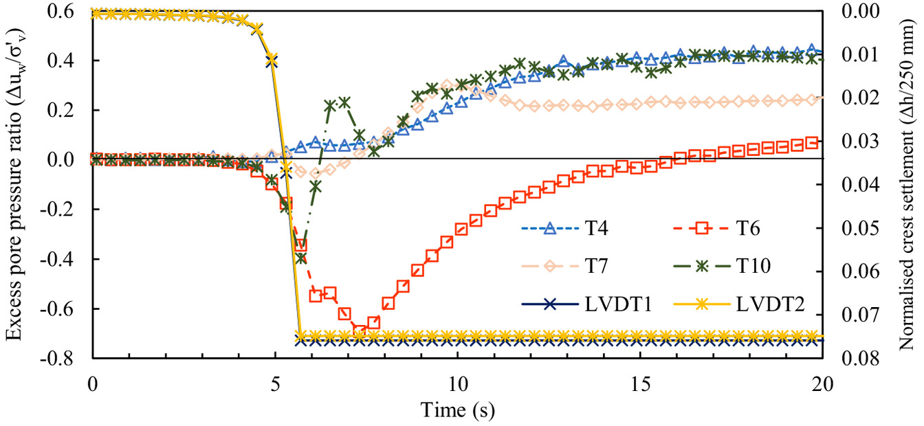
From Fig. 13 it can be seen that, as soon as crest settlements were measured, the tensiometers started to measure a change in pore pressures. Looking at the measured crest settlement, the collapse occurred fairly rapidly, as the crest settled more than 18 mm within 1 s. The slope actually experienced more settlement during this time, as the plateau of the measured crest settlements indicates the end of travel of the LVDTs. Similar to the measured pore pressure response in Test GT-1, the tensiometers initially measured a drop in pore pressure at the start of the failure event due to tension in the cables. The tensiometers were located close to the observed failure surface [Fig. 12(a)] and, as the soil mass moved, the cables of the tensiometers were pulled. However, positive excess pore pressures were measured soon after this initial dilation, indicating that the tailings had a contractive response during shearing. This fluctuation in measured pore pressures confirms that the failure of the sliding soil mass caused at least partial undrained shearing in the model slope.
Like what was observed in Test GT-1, T6 only measured negative excess pore pressures during the failure event. T6 measured a minimum (Fig. 13). The negative measured could be due to the tensiometer being pulled from the soil during the failure event. T4 and T10 measured the highest peak excess pore pressure ratios: and 54.2 kPa , respectively. T7 measured a peak . These peak values are lower than the largest peak measured in Test GT-1, for two reasons. First, the slope in Test GT-2 was prepared in a denser state than in Test GT-1. Thus, it can be expected that the magnitude of positive excess pore pressures generated will be smaller. Second, the failure in Test GT-2 has a slower peak rate of shearing than that in Test GT-1. As the soil was sheared, positive excess pore pressures were generated within the tailings. However, as the excess pore pressures were generated, some excess pore pressures dissipated. Owing to the slower rate of shearing, more excess pore pressures could dissipate during the failure event when compared with Test GT-1. However, it should be noted that, even if partial drainage was present, which would lead to the dissipation of positive excess pore pressures, soils that exhibit quasi steady state behavior, as well as strain softening behavior, can still result in liquefaction events (Jefferies and Been 2016).
Validation of Numerical Model
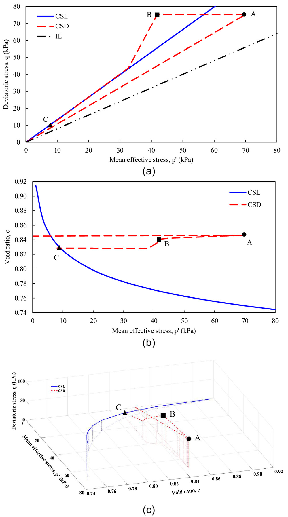
In order to validate the numerical model used for the numerical back-analysis of Test GT-2, a CSD stress path was simulated using the model shown in Fig. 14(a). Fig. 14 shows the simulated response of a CSD specimen with a at the start of unloading. Fig. 14(a) shows the simulated stress path in the plane. The soil was sheared anisotropically under drained conditions until Point A, using the Mohr-Coulomb model. This simulated the stress path that a soil element within a model slope experiences during centrifugal acceleration. The average IL for the gold tailings used is also plotted in Fig. 14(a), which shows that Point A is above the IL. After reaching Point A, the material model was switched to NorSand and the unloading process was started, subjecting the model to a CSD stress path. The mean effective stress continued to decrease until instability was triggered at Point B, at which the soil collapsed to Point C. Instability was only triggered at , which is above the CSL in the plane. This is due to the lack of an internal cap in the current NorSand implementation in PLAXIS 2D, which would limit the hardening of the yield surface if implemented (Jefferies 1997). However, Fig. 14(b) shows the soil response during the CSD simulation in the space. During unloading (from Point A to Point B), there was a slight contraction after the initiation of instability at Point B, followed by rapid undrained shearing and a collapse to Point C on the CSL. Fig. 14(c) shows the CSD simulation in the space along with the CSL. It is evident that the sudden contraction at Point B triggered the rapid collapse of the soil towards the CSL. During the collapse of the soil, there was a rapid accumulation of axial strain, which resulted in the undrained shearing of the soil. This rapid collapse and undrained shearing triggered the generation of 34 kPa of positive excess pore pressure, which ultimately resulted in the sudden loss of shear resistance of the soil. This behavior was consistent with specimens with positive values (i.e., contractive tendencies). For specimens with negative values (i.e., dilative tendencies), slower failures were observed with very little change in pore pressures.
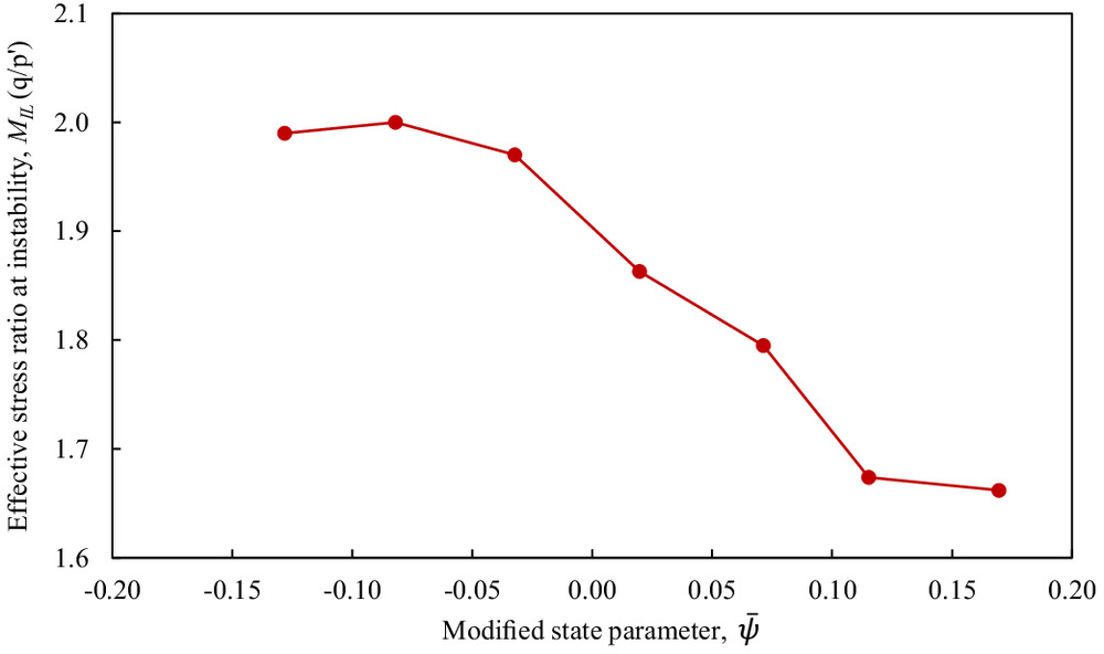
Adopting the relationship between the slope on the instability line and the modified state parameter (after Chu et al. 2003), a trend between the simulated versus the corresponding can be determined (Fig. 15). As shown in Fig. 15, the change in is relatively moderate for specimens with negative (dilative specimens), which corresponds to the work performed by Chu et al. (2003). A more drastic change in is observed for specimens with positive , which again is consistent with the common observation that the void ratio has a greater influence on the for loose specimens than for dense specimens (Chu et al. 2003). One thing to note is that the for all these simulations are higher than what we would expect from laboratory tests, which is due to the lack of an internal cap in the current NorSand implementation in PLAXIS 2D. Nevertheless, this indicates that the onset of instability during a CSD stress path can be predicted when using NorSand, albeit at a higher values.
Numerical Back-Analysis of Test GT-2
Based on the measured results and the video evidence of the failure event, it is hypothesized that the failure of the slope was a slide-to-flow failure (Bolton et al. 2003; Take et al. 2004). To confirm this hypothesized trigger and failure mechanism, a numerical back-analysis of Test GT-2 was conducted using the model shown in Fig. 4(b). In the back-analysis, a head of 280 mm was applied at the upstream end of the slope. The water was allowed to seep into the slope during the fully coupled, flow-deformation stage of the analysis, progressively raising the water table until the failure of the slope was triggered. Failure here is defined as when the solution failed to reach convergence. This is an indication that large plastic strains developed rapidly.
Fig. 16 shows the variations of normalized computed pore fluid pressures by with time at the monitored stress points over the duration of the entire test. Comparing Fig. 16 with Fig. 11(a), one notable difference between the numerical and physical models is that the numerical model is not able to capture well the downward migration of pore fluid and the associated increase in matric suction that occurs in the unsaturated zone under high acceleration. A gradual increase in suction was noted during the course of the test on data from tensiometers T1, T3, T4, and T5 installed in unsaturated tailings [Fig. 11(a)]. This increase in suction would have resulted from the downward migration of moisture under high acceleration, along with the tailings, and consequently the tensiometers, drying out over the approximately 1 h test duration. The air-entry value of the tensiometers was 50 kPa, implying that excessive dry-out would not have been accompanied by cavitation, which makes the identification of excessive dry-out difficult. As the water table rose during the test, the measured pore pressures increased, but to values less than predicted numerically. It is believed that this was the result of excessive dry-out and slow tensiometer resaturation as the phreatic surface rose, resulting in undermeasurement of pore pressures. However, the magnitude of the positive pore pressures in the saturated zones were better matched.
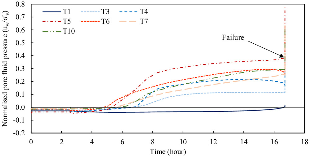
Fig. 17 shows the computed stress paths of all the monitored stress points during the numerical back-analysis. It can be seen that all of the monitored stress points were loaded anisotropically during Stage 2 of the numerical back-analysis. During this stage, the deviatoric stress and mean effective stress increased linearly at all points, with the computed stress ratio varying between 1.02 and 1.23, depending on the location within the slope. After the model reached the test acceleration level, wetting was initiated, and the fluid level was raised until the slope experienced instability. No change in the stress state was observed during the switch from the Mohr-Coulomb model to the NorSand model. T7 and T10 each experienced a slight decrease in deviatoric stress as the water table approached their location. It is possible that a certain amount of shear stress was mobilized during the acceleration stage. As the water table rose, the shear strength of the underlying material reduced somewhat first, resulting in the loss of some of the mobilized shear stress in the material overhead. Once the phreatic surface reached the location of these stress points, the effective stress started to reduce at a constant shear stress. The soil around the locations of T3, T4, T5, and T6 all experienced a slight decrease in mean effective stress once the phreatic surface reached their locations with an approximately constant deviatoric stress. Once the phreatic surface reached the location shown in Fig. 18, the slope collapsed. The initiation of instability is indicated by the triangular markers in Fig. 17. Once instability was triggered, the soil around T3, T4, T5, T6, T7, and T10 experienced a sudden reduction in mean effective stress, along with the rapid generation of shear strains and positive excess pore pressures (to be discussed), with a slight decrease in deviatoric stress. The soil around the location of T1 did not experience much change in the stress state, as it was located in the unsaturated zone above the phreatic surface (Fig. 18). At this point, the numerical back-analysis could not obtain convergence, due to the rapid generation of large shear strains, indicating a runaway slip failure. The stress state at the onset of instability denotes the state of the soil element at which it is no longer able to support the external shear stress imposed on it under undrained or partially undrained conditions (Ng et al. 2004). The soil elements experienced instability at different mobilized friction angles, ranging from 27.3° to 32.0°. At stress ratios above the IL, collapse is triggered due to a small change in the stress ratio, which leads to the triggering of instability within the slope.
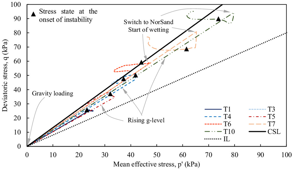
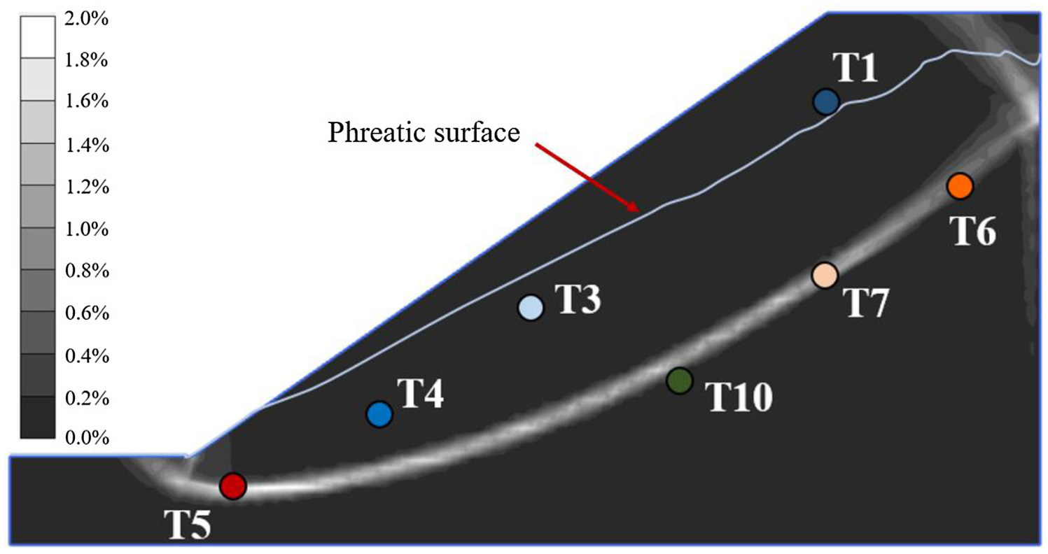
Fig. 18 shows the computed shear strain distribution during the failure of the slope. It can be seen that the location of the phreatic surface, which triggered the failure of the slope, is in good agreement with the observed phreatic surface just before failure in Test GT-2 [Fig. 12(a)]. In addition, the failure that was triggered during the back-analysis was a slide-to-flow failure like the failure observed in Test GT-2. Here, a conventional slip failure was predicted. The overall shape, depth and location of the slip failure is also similar to the observed slip failure from Test GT-2. The slip failure has an approximately logarithmic spiral shape that starts just past the toe, progresses upstream and extends slightly upstream of the crest of the slope. When comparing the observed failure surface [Fig. 12(a)] with the computed failure surface (Fig. 18), it can also be seen that the locations of the tensiometers relative to the failure surface are in good agreement with the physical model.
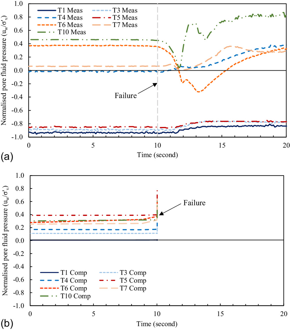
Figs. 19(a and b) respectively show the normalized pore fluid pressure response versus time around the time of failure at the monitored points in the physical and numerical models. The pore pressure responses at the time of failure are difficult to compare in detail because the numerical model can only yield values up to the point of nonconvergence. However, similar trends are seen up to that point, with pore pressures in both the physical and numerical models increasing. In addition, the computed pore pressures are generally higher than the measured pore pressures. As previously discussed, it is possible that the lower measured values are due to the dry-out and incomplete resaturation of the tensiometers. However, a qualitative comparison between the measured and computed pore pressures appears reasonable.
For comparison with the physical model, Fig. 20 shows the computed during the failure of the slope during the back-analysis of Test GT-2. During the numerical back-analysis, the predicted failure occurs instantaneously [Fig. 19(b)]. Thus, the computed is plotted against peak shear stain (e.g., deformation). It can be seen that for all the monitored stress points only a contractive response (i.e., positive excess pore pressures) was predicted during the numerical back-analysis. This is the major difference between the measured and computed values. The measured response of the slope first indicated a dilative response, which was followed by a contractive response (Fig. 13). As mentioned, it is possible that the shearing of the soil during the slope failure caused tension in the cables of the tensiometers. The tension can readily explain the initial dilation. However, shortly after the initial dilation, positive excess pore pressures were generated.
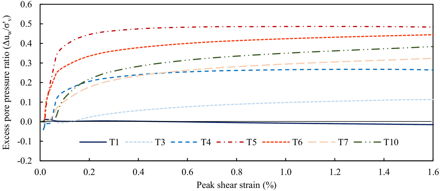
During Test GT-2, T4 and T10 measured the peak values, reaching an of 0.44 and 0.42, respectively (Fig. 13). The computed peak at T4 and T10 were 0.28 and 0.39, respectively (Fig. 20). The computed at T4 is somewhat less than the measured, possibly due to the location of T4. As T4 was situated above the failure surface, the soil around T4 experienced a lesser amount of shearing, which would cause smaller excess pore pressures to be generated. The computed at T10 is close to the measured value. Furthermore, the computed at T7 reached a peak value of 0.33, which is also close to the measured of 0.30.
T5 did not measure any significant changes in the pore fluid pressure during the slope failure in Test GT-2. The measured value of T5 at the time of failure indicated that the soil was still unsaturated. As the seepage in Test GT-2 happened much quicker than in Test GT-1, it is possible that the soil around the toe of the slope was partially saturated. Another reason could be that T5 dried before the fluid level reached T5, thus showing a slow response. The numerical back-analysis of Test GT-2 indicated that the soil at the toe of the slope (around T5) should have been fully saturated and have experienced the largest amount of shearing during the failure event (Fig. 18). This is confirmed by the computed at T5, which reached a value of 0.49, which is the largest computed in the slope during the failure event.
The computed at T6 also differs from the measured value. During Test GT-2, T6 measured only negative excess pore pressures (Fig. 13). The cable of T6 passed through the soil mass that failed in Test GT-2, which caused tension in the cable, which would have generated negative excess pore pressures. During the back-analysis of Test GT-2, T6 reached a peak computed of 0.45. The failure caused the undrained shearing of the soil in close proximity to the slip surface, which caused positive excess pore pressures to be generated. Like the measured , negligible changes in the pore pressure during the failure of the slope were computed for T1 and T3.
As mentioned, consolidation can lead to shear densification within the slope. To study the impact of shear densification on the instability behavior of the model, two additional analyses were conducted using the same methodology as the numerical back analysis of Test GT-2, but with values of 0.03 and 0.06. During both analyses the slopes failed when the phreatic surface was approximately in the same location as that shown in Fig. 18, only slightly higher. The overall shape and depth of the slip surfaces during both analyses were also similar to those shown in Fig. 18. The pore pressure responses during failure for both analyses were also similar to those computed during the back analysis of Test GT-2 (Fig. 20). During both analyses positive excess pore pressures were generated during the failure events due to the triggering of undrained shearing, indicating a decrease in shear strength. However, the magnitudes of excess pore pressures generated were reduced.
For the analysis with , the peak values at T4, T5, and T6 reduced by between 19% and 23%, compared with the analysis with . The values at T7 and T10 reduced by 28% and 29%, respectively. For the analysis with , the peak at T5 reduced by 25%, whereas at T4, T6, T7, and T8 the values reduced by between 48% and 55% when compared with the analysis with .
These analyses indicate that shear densification will result in lower peak values. However, as the values were still positive (i.e., the soil has a contractive tendency), the positive excess pore pressures generated during the failure events still resulted in a reduction in shear strength, causing a slide-to-flow failure.
Considering the observed and computed failure mechanisms, as well as the measured and computed values during the failure of GT-2, it can be concluded that the rising water table triggered the drained failure of the slope, which in turn triggered the undrained shearing of the soil. This undrained shearing caused the generation of positive excess pore pressures, which reduced the effective stress. This reduction in effective stress caused a decrease in the shear strength of the soil, especially along the slip surface, which led to the failure of the slope. Based on the observed and predicted failure mechanisms (Figs. 12 and 18), it can be concluded that the slope in Test GT-2 experienced a slide-to-flow failure, similar to that described by Bolton et al. (2003) and Take et al. (2004). It should be pointed out that, although a drained slope stability analysis would predict this specific trigger and subsequent failure, tailings storage facilities with adequate drained factors of safety might have inadequate undrained factors of safety when subjected to a trigger capable of initiating an undrained response.
For interest’s sake, the yield strength ratio [] at which failure occurred was determined, after Olson and Stark 2003. Here is the peak shear strength available during undrained loading and the pre-failure vertical effective stress. Although not strictly applicable, as the failure trigger was drained instability followed by undrained shearing post failure, an equivalent of 0.54 was calculated for Test GT-2. This value is much higher than the typical range of values found by Olson and Stark (2003), as the failure was not the result of undrained instability.
Summary and Conclusions
Based on two centrifuge model tests and a finite element analysis on gold tailings dams, potential triggers and failure mechanisms of flow failures were investigated and described. Flow and slide failures were triggered in the centrifuge tests by raising the groundwater table using a viscous fluid. The centrifuge tests approximately replicated CSD stress paths, where the effective stress is reduced whilst maintaining a constant deviatoric stress. The high pore pressures and large seepage forces at the toe of the slope, in combination with its loose state, resulted in sloughing at the toe in the first test (GT-1). The sloughing eventually caused a soil mass to break away, which acted as a monotonic unloading trigger. This resulted in shearing of the loose contractile saturated soil at the toe of the slope. The failure triggered localized liquefaction at the toe, indicated by a measured , causing a loss of shear strength. The toe of the slope could not support the upstream material and a retrogressive flowslide failure was triggered. During the rapid flowslide, positive excess pore pressures were generated throughout the rest of the slope. The positive excess pore pressures reduced the effective stress in the slope, triggering further instability, which resulted in a liquefaction failure.
In the second test (GT-2), drained instability triggered a slip failure as pore pressures gradually increased due to the rising fluid level. This resulted in a CSD stress path. This drained trigger resulted in undrained or at least partially undrained shearing of the soil within the slope, which caused positive excess pore pressures to be generated, reducing the shear strength of the tailings. The rate of shearing was slower compared to the eventual flow slide in the first test. This allowed for some positive excess pore pressures to dissipate, resulting in a lower measured peak of 0.44 to be mobilised. A slide-to-flow failure was triggered.
CSD stress paths were simulated using a calibrated NorSand model to verify whether the model is capable of predicting instability under these conditions. These simulations indicate that the NorSand model is capable of predicting the onset of instability during a CSD stress path, albeit at higher values than what would be expected. This is due to the lack of an internal cap in the current implementation of NorSand, which controls the maximum dilatancy of the soil. These simulations also confirm that NorSand is capable of predicting the transition from drained instability to undrained shearing.
The numerical back-analysis of Test GT-2 confirmed that the rising water table resulted in a CSD stress path, ultimately triggering a slip failure due to drained instability. The drained instability triggered the undrained shearing within the slope. The undrained shearing caused the generation of positive excess pore pressures, which resulted in a loss of shear strength and triggered a slide-to-flow failure. This specific failure would have been predicted with a conventional drained slope stability analysis.
Data Availability Statement
Some or all data, models, or code generated or used during the study are available from the corresponding author by request.
Acknowledgments
The authors would like to acknowledge the funding support provided by the Research Grants Council of the Hong Kong Special Administrative Region, China (Project Nos. AoE/E-603/18, 16212618, and 16209717). The authors are also grateful for the financial sponsorship from the National Natural Science Foundation of China (No. 51709052).
References
Askarinejad, A., A. Beck, and S. M. Springman. 2014. “Scaling law of static liquefaction mechanism in geocentrifuge and corresponding hydromechanical characterization of an unsaturated silty sand having a viscous pore fluid.” Can. Geotech. J. 52 (6): 708–720. https://doi.org/10.1139/cgj-2014-0237.
Azam, S., and Q. Li. 2010. “Tailings dam failures: A review of the last one hundred years.” Geotech. News 28 (4): 50–54.
Bishop, A. W. 1966. “Strength of soils as engineering materials, Sixth Rankine lecture.” Géotechnique 16 (2): 89–130. https://doi.org/10.1680/geot.1966.16.2.91.
Bolton, M. D., W. A. Take, P. C. P. Wong, and F. J. Yeung. 2003. “Mechanisms of failure in fill slopes after intense rainfall.” In Vol. 1 of Proc., Int. Conf. on Slope Engineering, 1–25. London: International Society for Soil Mechanics and Geotechnical Engineering.
Cai, Z. Y. 2001. “A comprehensive study of state-dependent dilatancy and its application in shear band formation analysis.” Ph.D. thesis, Dept. of Civil Engineering, Hong Kong Univ. of Science and Technology.
Castro, G. 1969. “Liquefaction of sands.” Ph.D. thesis, Division of Engineering and Applied Physics, Harvard Univ.
Chang, N., G. Heymann, and C. Clayton. 2011. “The effect of fabric on the behaviour of gold tailings.” Géotechnique 61 (3): 187–197. https://doi.org/10.1680/geot.9.P.066.
Chang, N. Y., N. P. Hseih, D. L. Samuelson, and M. Horita. 1981. “Static and cyclic behaviour of Monterey #0 sand.” In Proc., 3rd Microzonation Conf., 929–944. Alexandria, VA: National Science Foundation.
Chu, J., S. Leroueil, and W. K. Leong. 2003. “Unstable behaviour of sand and its implication for slope instability.” Can. Geotech. J. 40 (5): 873–885. https://doi.org/10.1139/t03-039.
CIMNE (Centro Internacional de Métodos Numéricos en la Ingeniería). 2021. “Computational analyses of Dam I failure at the Corrego de Feijao mine Brumadinho: Final report.” Accessed January 14, 2022. http://www.mpf.mp.br/mg/sala-de-imprensa/docs/2021/relatorio-final-cinme-upc-1.
Crous, P. A., C. W. W. Ng, and S. W. Jacobsz. 2022. “Lessons learnt modelling tailings dam flow-type failures in the centrifuge.” In Proc., 10th Int. Conf. on Physical Modelling in Geotechnics, 281–284, London: International Society for Soil Mechanics and Geotechnical Engineering.
Cuomo, S., P. Ghasemi, M. Martinelli, and M. Calvello. 2019. “Simulation of liquefaction and retrogressive slope failure in loose coarse-grained material.” Int. J. Geomech. 19 (10): 04019116. https://doi.org/10.1061/(ASCE)GM.1943-5622.0001500.
do Carmo, F. F., et al. 2017. “Fundao tailings dam failures: The environmental tragedy of the largest technological disaster of Brazilian mining in global context.” Perspect. Ecol. Conserv. 15 (3): 145–151. https://doi.org/10.1016/j.pecon.2017.06.002.
Eckersley, D. 1990. “Instrumented laboratory flowslides.” Géotechnique 40 (3): 489–502. https://doi.org/10.1680/geot.1990.40.3.489.
Fourie, A. B., G. E. Blight, and G. Papageorgiou. 2001. “Static liquefaction as a possible explanation for the Merriespruit tailings dam failure.” Can. Geotech. J. 38 (4): 707–719. https://doi.org/10.1139/t00-112.
Hazen, A. 1930. “Water supply.” In American civil engineers handbook. New York: Wiley.
Ishihara, K. 1993. “Liquefaction and flow failure during earthquakes.” Géotechnique 43 (3): 351–451. https://doi.org/10.1680/geot.1993.43.3.351.
Jacobsz, S. W. 2018. “Low cost tensiometers for geotechnical applications.” In Proc., 9th Int. Conf. on Physical Modelling in Geotechnics, 305–310. Boca Raton, FL: CRC Press.
Jacobsz, S. W., E. P. Kearsley, and J. H. L. Kock. 2014. “The geotechnical centrifuge facility at the University of Pretoria.” In Proc., 8th Int. Conf. on Physical Modelling in Geotechnics. London: International Society for Soil Mechanics and Geotechnical Engineering. https://doi.org/10.1201/b16200-16.
Jefferies, M. G. 1993. “Nor-Sand: A simple critical state model for sand.” Géotechnique 43 (1): 91–103. https://doi.org/10.1680/geot.1993.43.1.91.
Jefferies, M. G. 1997. “Plastic work and isotropic softening in unloading.” Géotechnique 47 (5): 1037–1042. https://doi.org/10.1680/geot.1997.47.5.1037.
Jefferies, M. G., and K. Been. 2016. Soil liquefaction: A critical state approach. 2nd ed. Boca Raton, FL: CRC Press. https://doi.org/10.1201/b19114.
Jefferies, M. G., N. R. Morgernstern, D. V. van Zyl, and J. Wates. 2019. Report on NTSF embankment failure. South Orange, NSW, Australia: Valley Operations for Ashurst Operations.
Jennings, J. E. B., and J. B. Burland. 1962. “Limitations to the use of effective stresses in partly saturated soils.” Géotechnique 12 (2): 125–144. https://doi.org/10.1680/geot.1962.12.2.125.
Kennedy, R., W. A. Take, and G. Siemens. 2020. “Geotechnical centrifuge modelling of retrogressive sensitive clay landslides.” Can. Geotech. J. 58 (10): 1452–1465. https://doi.org/10.1139/cgj-2019-0677.
Konrad, J. M. 1990. “Minimum undrained strength of two sands.” J. Geotech. Eng. 116 (6): 932–947. https://doi.org/10.1061/(ASCE)0733-9410(1990)116:6(932).
Kramer, S. L., and H. B. Seed. 1988. “Initiation of soil liquefaction under static loading conditions.” J. Geotech. Eng. 114 (4): 412–430. https://doi.org/10.1061/(ASCE)0733-9410(1988)114:4(412).
Lade, P. V. 1992. “Static instability and liquefaction of loose fine sandy slopes.” J. Geotech. Eng. 118 (1): 51–71. https://doi.org/10.1061/(ASCE)0733-9410(1992)118:1(51).
Lade, P. V., and J. A. Yamamuro. 2011. “Evaluation of static liquefaction potential of silty sand slopes.” Can. Geotech. J. 48 (2): 247–264. https://doi.org/10.1139/T10-063.
Mànica, M. A., M. Arroyo, A. Gens, and L. Monforte. 2022. “Application of a critical state model to the Merriespruit tailings dam failure.” Proc. Inst. Civ. Eng. Geotech. Eng. 175 (2): 151–165. https://doi.org/10.1680/jgeen.21.00001.
Morgernstern, N. R., S. G. Vick, C. B. Viotti, and B. D. Watts. 2016. Fundão tailings dam review panel. New York: World Press.
Moriwaki, H., T. Inokuchi, T. Hattanji, K. Sassa, H. Ochiai, and G. Wang. 2004. “Failure processes in a full-scale landslide experiment using a rainfall simulator.” Landslides 1 (4): 277–288. https://doi.org/10.1007/s10346-004-0034-0.
Ng, C. W. W., C. F. Chiu, and C. K. Shen. 1998. “Effects of wetting history on the volumetric deformations of an unsaturated loose fill.” In Vol. 1 of Proc., 13th Southeast Asian Geotechnical Conf., 141–146. Taipei, Taiwan: Southeast Asian Geotechnical Society.
Ng, C. W. W., P. A. Crous, M. Zhang, and M. Shakeel. 2022. “Static liquefaction mechanisms in loose sand fill slopes.” Comput. Geotech. 141 (Jan): 104525. https://doi.org/10.1016/j.compgeo.2021.104525.
Ng, C. W. W., W. T. Fung, C. Y. Cheuk, and L. Zhang. 2004. “Influence of stress ratio and stress path on behavior of loose decomposed granite.” J. Geotech. Geoenviron. Eng. 130 (1): 36–44. https://doi.org/10.1061/(ASCE)1090-0241(2004)130:1(36).
Olson, S. M., and T. D. Stark. 2003. “Yield strength ratio and liquefaction analysis of slopes and embankments.” J. Geotech. Geoenviron. Eng. 129 (8): 727–737. https://doi.org/10.1061/(ASCE)1090-0241(2003)129:8(727).
Poulose, A., S. R. Nair, and D. N. Singh. 2000. “Centrifuge modelling of moisture migration in silty soils.” J. Geotech. Geoenviron. Eng. 126 (8): 748–752. https://doi.org/10.1061/(ASCE)1090-0241(2000)126:8(748).
Reid, D., and R. Fanni. 2022. “A comparison of intact and reconstituted samples of a silt tailings.” Géotechnique 72 (2): 176–188. https://doi.org/10.1680/jgeot.20.P.020.
Reid, D., R. Fanni, and P. DiDonna. 2022. “The effect of tamping conditions on undrained shear strengths of a non-plastic sandy silt tailings.” Can. Geotech. J. 59 (6): 783–795. https://doi.org/10.1139/cgj-2020-0269.
Reid, D., and K. Smith. 2021. “Interpretation of state parameter in partially drained tailings: A case history examination.” Géotech. Lett. 11 (4): 276–280. https://doi.org/10.1680/jgele.21.00066.
Riveros, G. A., and A. Sadrekarimi. 2021. “Static liquefaction behaviour of gold mine tailings.” Can. Geotech. J. 58 (6): 889–901. https://doi.org/10.1139/cgj-2020-0209.
Robertson, P. K., L. de Melo, D. J. Williams, and G. W. Wilson. 2019. “Report of the expert panel on the technical causes of the failure of Feijão Dam I.” Accessed January 28, 2020. http://www.b1technicalinvestigation.com/.
Sasitharan, S., P. K. Robertson, D. C. Sego, and N. R. Morgernstern. 1993. “Collapse behavior of sand.” Can. Geotech. J. 30 (4): 569–577. https://doi.org/10.1139/t93-049.
Shuttle, D., and M. Jefferies. 2010. NorSand: Description, calibration, validation and applications. Reston, VA: ASCE.
Shuttle, D., and M. Jefferies. 2016. “Determining silt state from CPTu.” Geotech. Res. 3 (3): 90–118. https://doi.org/10.1680/jgere.16.00008.
Skopek, P., N. R. Morgernstern, P. K. Robertson, and K. C. Sego. 1994. “Collapse of dry sand.” Can. Geotech. J. 31 (6): 1008–1014. https://doi.org/10.1139/t94-115.
Sladen, J. A., R. D. D’Hollander, and J. Krahn. 1985. “The liquefaction of sands, a collapse surface approach.” Can. Geotech. J. 22 (4): 564–578. https://doi.org/10.1139/t85-076.
Take, W. A. 2014. “Keynote paper: Current and emerging physical modelling technologies.” In Proc., 8th Int. Conf. on Physical Modelling in Geotechnics. London: International Society for Soil Mechanics and Geotechnical Engineering.
Take, W. A., and R. A. Beddoe. 2014. “Base liquefaction: A mechanism for shear-induced failure of loose granular slopes.” Can. Geotech. J. 51 (5): 496–507. https://doi.org/10.1139/cgj-2012-0457.
Take, W. A., R. A. Beddoe, R. Davoodi-Bilesavar, and R. Phillips. 2015. “Effect of antecedent groundwater conditions on the triggering of static liquefaction landslides.” Landslides 12 (3): 469–479. https://doi.org/10.1007/s10346-014-0496-7.
Take, W. A., M. D. Bolton, P. C. P. Wong, and F. J. Yeung. 2004. “Evaluation of landslide triggering mechanisms in model fill slopes.” Landslides 1 (3): 173–184. https://doi.org/10.1007/s10346-004-0025-1.
Theron, M., C. R. I. Clayton, and G. Heymann. 2004. “The small strain stiffness of gold tailings.” In Proc., ISC-2 on Geotechnical and Geophysical Site Characterization, 575–580. Rotterdam, Netherlands: Millpress.
Vaid, Y. P., and S. Sivathayalan. 2000. “Fundamental factors affecting liquefaction susceptibility of sands.” Can. Geotech. J. 37 (3): 592–606. https://doi.org/10.1139/t00-040.
Wagener, F. 1997. “The Merriespruit slimes dam failure: Overview and lessons learned.” J. South Afr. Inst. Civ. Eng. 39 (3): 11–15.
Wagener, F., H. J. Craig, G. E. Blight, G. McPhail, A. A. B. Williams, and J. H. Strydom. 1998. “The Merriespruit tailings dam failure—A review.” In Proc., of the Conf. on Tailings and Mine Waste, 925–952. Fort Collins, CO: Colorado State Univ.
Wang, G., and K. Sassa. 2000. “Effects of grain size on sliding surface liquefaction behaviour of sands based on ring shear tests. Landslides in research, theory and practice.” In Proc., 8th Int. Symp. on Landslides, 1539–1544. London: Institution for Civil Engineers.
Woudstra, L. J. 2021. “Verification, validation and application of the NorSand constitutive model in PLAXIS.” Master’s thesis, Faculty of Civil Engineering and Geo-Sciences, Delft Univ. of Technology.
Yang, J. 2002. “Non-uniqueness of flow liquefaction line for loose sand.” Géotechnique 52 (10): 757–760. https://doi.org/10.1680/geot.2002.52.10.757.
Zhang, W., and A. Askarinejad. 2021. “Centrifuge modelling of static liquefaction in submarine slopes: Scaling law dilemma.” Can. Geotech. J. 58 (2): 200–209. https://doi.org/10.1139/cgj-2019-0417.
Information & Authors
Information
Published In

Journal of Geotechnical and Geoenvironmental Engineering
Volume 149 • Issue 9 • September 2023
Copyright
This work is made available under the terms of the Creative Commons Attribution 4.0 International license, https://creativecommons.org/licenses/by/4.0/.
History
Received: Feb 11, 2022
Accepted: Apr 18, 2023
Published online: Jun 27, 2023
Published in print: Sep 1, 2023
Discussion open until: Nov 27, 2023
Authors
Metrics & Citations
Metrics
Citations
Download citation
If you have the appropriate software installed, you can download article citation data to the citation manager of your choice. Simply select your manager software from the list below and click Download.
Cited by
- Ali P. Babaki, Dwayne D. Tannant, Numerical Evaluation of Static Liquefaction–Induced Flowslide Causing the Edenville Dam Failure, Michigan, Journal of Geotechnical and Geoenvironmental Engineering, 10.1061/JGGEFK.GTENG-11998, 150, 5, (2024).