Revised Soil Classification System: Implementation and Engineering Implications

Castro, Gloria M.; Park, Junghee; Santamarina, J. Carlos

doi:10.1061/JGGEFK.GTENG-10447

Open access

Technical Papers

Sep 13, 2023

Revised Soil Classification System: Implementation and Engineering Implications

Authors: Gloria M. Castro https://orcid.org/0000-0002-2667-1801, Junghee Park https://orcid.org/0000-0001-7033-4653 [email protected], and J. Carlos Santamarina, A.M.ASCE https://orcid.org/0000-0001-8708-2827Author Affiliations

Publication: Journal of Geotechnical and Geoenvironmental Engineering

Volume 149, Issue 11

https://doi.org/10.1061/JGGEFK.GTENG-10447

PDF

Abstract

Soil classification systems help geotechnical engineers anticipate soil properties and provide early guidance for engineering analyses. Current soil classification systems recognize the central role of particle size and inherent differences between coarse- and fine-grained fractions. However, they adopt fixed classification boundaries irrespective of a broad range of fines plasticity and particle shape, disregard the distinct fines thresholds for mechanical and hydraulic properties, and overlook pore-fluid chemistry effects on fines behavior. The Revised Soil Classification System (RSCS) addresses these limitations and benefits from published data and physical insights gained during the last century. By comparison, the classification boundaries in the prevailing Unified Soil Classification System (USCS) resemble those in the RSCS only for the case of angular sands and gravels mixed with low-plasticity fines; in all other cases, extensive data sets corroborate the transition thresholds adopted in the RSCS. The complete logic tree for the RSCS facilitates its implementation; it is available as user-friendly Excel macro and a mobile application that automatically produce the soil-specific classification charts and show the soil classification in terms of the controlling fraction for both mechanical and hydraulic properties. Multiple studies have demonstrated the predictive power of the RSCS in terms of soil properties (e.g., compressibility, strength, hydraulic conductivity, and capillarity), soil phenomena (e.g., fines migration and bioactivity), and the preliminary selection of geotechnical solutions (e.g., soil improvement).

Introduction

Current soil classification systems capture early efforts to understand soil behavior and properties. Most classification systems recognize the central role of particle size

d

because it determines the balance between particle-level forces. Capillary and/or electrical forces gain relevance and control fabric formation when the grain size is less than

75 μm

(Santamarina 2003; Mitchell and Soga 2005); hence, Atterberg limits are valuable for the characterization of fine-grained soils (finer than

75 μm

). Conversely, particle shape and relative size—i.e., coefficient of uniformity

C_{u}

—determine fabric and packing density in coarse-grained soils (coarser than

75 μm

; Cho et al. 2006).

Classification systems developed in the 1930s have common limitations (Casagrande 1948; Burmister 1951; Wagner 1957; Holtz and Kovacs 1981; Howard 1984; Kulhawy and Chen 2009; Jang and Santamarina 2016; Park and Santamarina 2017): (1) they adopt a fixed boundary to distinguish coarse soils from fine-dominant soils regardless of a broad range of fines plasticity, (2) the shape of coarse-grained particles is not considered by any classification system, (3) boundaries in current classification systems do not recognize the distinct effects of fines on mechanical and hydraulic properties, and (4) current soil classification systems disregard the critical role of pore-fluid chemistry on the behavior of fine-grained sediments.

The recently proposed Revised Soil Classification System (RSCS) addresses these limitations, benefits from the physical understanding of granular materials gained in the field during the last century, and takes into consideration extensive data sets compiled from the geotechnical literature. This manuscript describes the implementation of the RSCS and demonstrates its valuable engineering implications.

Fundamental Concepts Involved in the RSCS

Coarse–Fines Mixtures

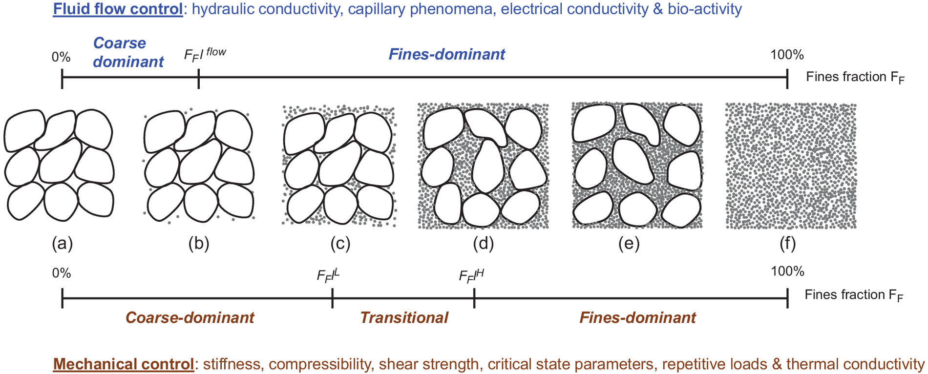
The RSCS defines two threshold fines fractions to classify coarse–fines mixtures into three categories: coarse-controlled, transitional, and fines-controlled mixtures (Fig. 1). The low-threshold fines fraction indicates the minimum amount of fines needed to fill the voids in a granular skeleton made by the coarse grains and it is attained when the coarse fraction is densely packed (

e_{C}^{\min}

) and the fines are loosely packed

(e_{F}^{\max)}, F_{F} |^{L} = e_{C}^{\min} / (1 + e_{C}^{\min} + e_{F}^{\max})

. Conversely, the high-threshold fines fraction is

F_{F} |^{H} = e_{C}^{\max} / (1 + e_{C}^{\max} + e_{F}^{\min})

, in which the coarse grains are loosely packed (

e_{C}^{\max}

) and the fines fraction is densely packed (

e_{F}^{\min}

) (Park and Santamarina 2017).

Fig. 1. RSCS transition thresholds. The corresponding gravimetric ratios were computed in terms of the extreme packing conditions for each fraction (details in Appendix I, II, and III). (Reprinted from Park and Santamarina 2017, © ASCE.)

Coarse Fraction

The packing void ratios

e^{\min}

and

e^{\max}

for coarse-grained sands and gravels can be measured readily (preferred) or estimated from particle roundness

R

and the coefficient of uniformity

C_{u}

(Appendix I); the maximum and minimum void ratios decrease for rounder and well-graded sands and gravels (Youd 1973; Cho et al. 2006). Experimental data revealed that coarse grains held in a fines matrix affect the physical properties of the mixture even beyond

e_{C} > e^{\max}

both in coarse–fines and gravel–sand mixtures (see data in Fragaszy et al. 1992; Vallejo and Mawby 2000; Vallejo 2001; Simoni and Houlsby 2006; Kim et al. 2007). Thus, the RSCS adopts a data-informed empirical correction for the high-threshold fines fraction

F_{F} |^{H^{*}} = α \cdot e_{C}^{\max} / (1 + α \cdot e_{C}^{\max} + e_{F}^{\min})

[Fig. 1(d)]. From the analysis of data gathered for various physical properties, we concluded that

α = 1.3

for coarse fines mixtures, and

α = 2.5

for gravel sand mixtures (see data collection in Park and Santamarina 2017).

Fines Fraction

The void ratio of plastic fine-grained soils (remolded) effectively is stress-dependent; therefore, the RSCS selects the void ratios measured in one-dimensional (1D) consolidation tests at

σ^{'} = 10 kPa

(

e^{\max} = e_{F} |^{10 kPa}

) and at

σ^{'} = 1 MPa

(

e^{\min} = e_{F} |^{1 MPa}

) as representative void ratios for soft and stiff conditions; the selection of alternative stress levels is discussed subsequently. These two values can be determined from a consolidation test using remolded specimens (although this is time demanding) or estimated from correlations with the liquid limit (LL) typically gathered with the saturating pore fluid (see correlations in Appendix II). Data sets in Skempton and Jones (1944); Skempton (1970); Burland (1990); and Chong and Santamarina (2016) confirm the strong correlation between the liquid limit and compression index

C_{c}

.

Fluid Transport Control Boundary

The presence of fines plays a critical role in permeability. The RSCS estimates the threshold fines fraction for fluid flow assuming that fines form a suspension with a viscosity 100 times higher than that of water, hence causing a marked decrease in the mixture hydraulic conductivity. Experimental data show that the suspension water content is several times higher than the liquid limit,

ω % = λ \cdot LL

, or, in terms of void ratio,

e_{F} |^{flow} = λ \cdot e_{F} |^{LL}

, where

λ = 2

for silt (

LL = 30 - 50

),

λ = 3

for kaolinite (

LL = 30 - 140

),

λ = 4

for illite (

LL = 90 - 210

), and

λ = 5

for bentonite (

LL = 170 - 300

). Clearly, the

λ

-factor scales with the liquid limit obtained with the saturating pore fluid, and it is best estimated as

λ = [2 \cdot \log (LL - 25)] \geq 1.0

. Details were presented by Park and Santamarina (2017).

RSCS Boundaries

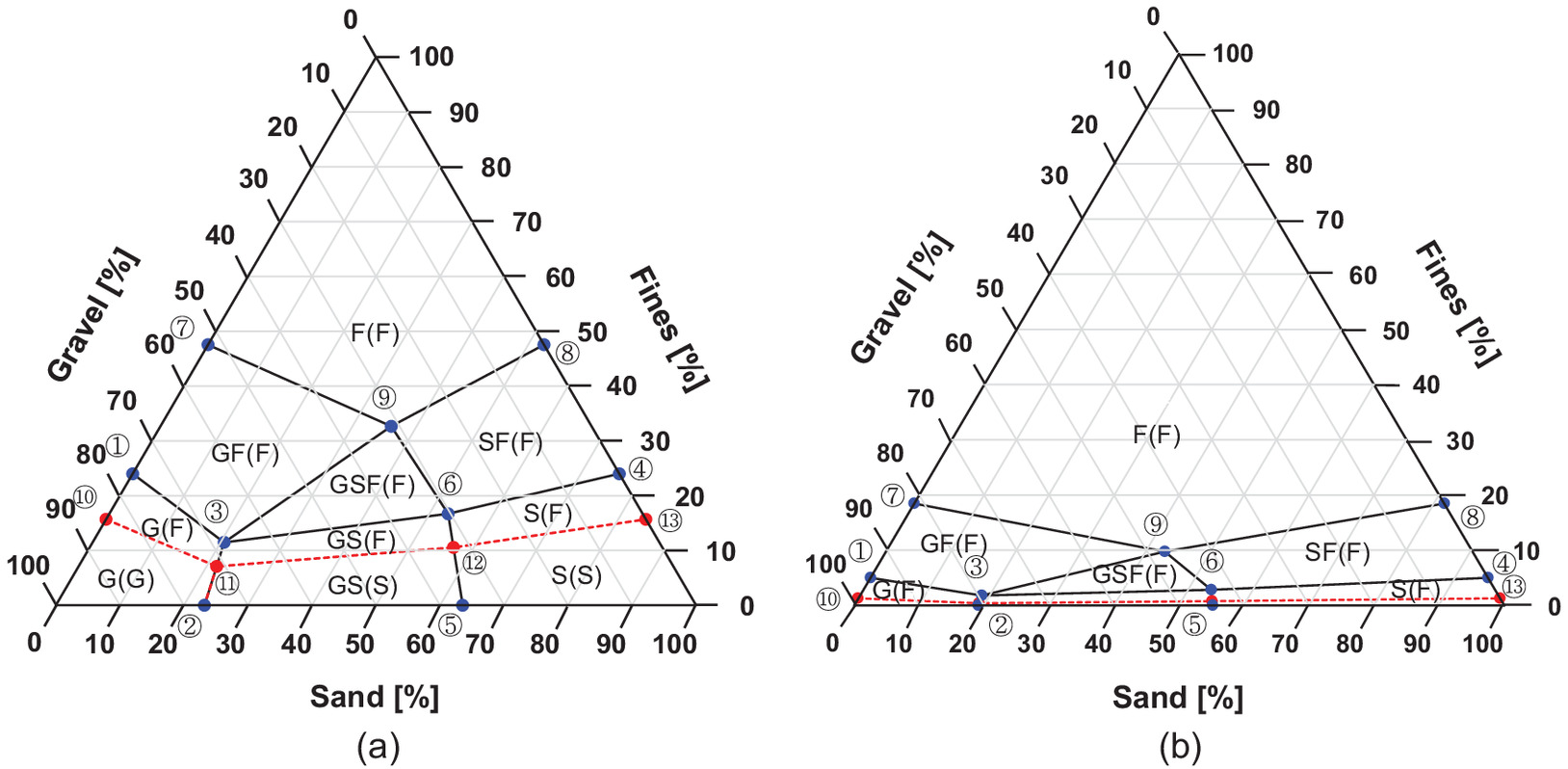
The 13 notable mixtures described in Appendix III define the RSCS boundaries. These boundaries constrain 10 soil groups in a textural triangular chart (Fig. 2). Each group has a two-name nomenclature: the first letter(s) identifies the component that controls the mechanical properties, and the second letter indicates the component that controls fluid flow (Fig. 2). For example, if the soil under consideration falls into the S(F) zone, it will exhibit sand-controlled mechanical properties but fines-controlled permeability.

Fig. 2. Revised Soil Classification System in the triangular gravel–sand–fines chart: (a) RSCS chart for a mixture of low-plasticity fines ( $LL = 40$ ), angular gravel, and sand (Roundness $R = 0.2$ , coefficient of uniformity $C_{u} = 1.5$ , $e^{\max} = 1.15$ , and $e^{\min} = 0.65$ ); and (b) RSCS chart for a mixture of high-plasticity fines ( $LL = 250$ ) and rounded gravel and sand ( $R = 0.5$ , $C_{u} = 1.5$ , $e^{\max} = 0.69$ , and $e^{\min} = 0.40$ ).

Comparison of RSCS and USCS

The Unified Soil Classification System (USCS) boundaries are similar to the RSCS triangular chart for angular sands and gravels mixed with low-plasticity fines, i.e., liquid limit

LL \approx 40

[Fig. 2(a)]. However, higher-plasticity fines and/or rounded coarse grains result in lower boundaries for both mechanical and hydraulic controls [Fig. 2(b)]. These sample charts capture the remarkable differences between the RSCS and the USCS; in particular, the RSCS boundaries are not fixed but are soil-specific in order to reflect properly the plasticity of fines and the shape of the coarse-grained fraction. In general, classification boundaries in the RSCS move down as the fines liquid limit increases and the coarse fraction roundness and uniformity increase. Park and Santamarina (2017) Fig. 10 presents multiple combinations of

R

,

C_{u}

, and LL.

Fines Classification

The most salient characteristic of fine-grained soils is their sensitivity to pore-fluid chemistry. Therefore, the RSCS classifies fines based on the liquid limit LL measured using the fall cone method for soil pastes prepared with three different liquids [Appendix IV and (Jang and Santamarina 2016)]: (1) the

{LL}_{DW}

run with deionized water magnifies double-layer effects and prevents the formation of face-to-face aggregation; (2) the

{LL}_{\ker}

obtained with nonpolar kerosene prevents hydration and osmotic effects, and thus van der Waals interparticle attraction prevails; and (3) the

{LL}_{brine}

conducted with a 2-M NaCl brine collapses the double layers. The choice of 2-M NaCl solution takes into consideration most saltwater bodies (

ocean water = 0.6 M

) and brine-filled reservoirs, prevents salt precipitation during testing (

saturation = 6.14 M

), effectively shields surface charges, minimizes double-layer effects, and is prepared easily.

The three liquid limits

{LL}_{DW}

,

{LL}_{brine}

, and

{LL}_{\ker}

render two ratios

{LL}_{\ker} / {LL}_{brine}

and

{LL}_{DW} / {LL}_{brine}

that capture the fabric sensitivity to the fluid electrical conductivity and permittivity [Appendix IV; Fig. 3(a)]. The liquid limit ratio

{LL}_{DW} / {LL}_{brine}

characterizes the reduction in double-layer thickness due to the increase in pore-fluid conductivity (

{LL}_{DW} > {LL}_{brine}

in most soils), and the ratio

{LL}_{\ker} / {LL}_{brine}

assesses changes in fines behavior due to changes in fluid permittivity (see data compilation in Santamarina et al. 2001, 2002).

Fig. 3. Fines classification based on the sensitivity to pore-fluid chemistry: (a) circular boundaries correspond to electrical sensitivities $S_{E} = 0.4$ (red) and $S_{E} = 1.0$ (blue); and (b) the two-letter nomenclature for fines classification indicates soil plasticity (N, L, I, or H) and electrical sensitivity (L, I, or H). Colored datapoints correspond to different soils identified in the legend.

We selected kerosene for its common availability worldwide; however, its composition is variable, heavier components may require days to evaporate, and its sale is banned in some countries (e.g., Peru). Other nonpolar fluids can be used; in particular, decane is a low-viscosity monomolecular liquid with convenient evaporation rate for laboratory testing. Experimental results in Fig. S1 in the Supplemental Materials summarize the liquid limit measurements for soil pastes prepared with kerosene and decane; the results confirm the potential use of either fluid to obtain the representative liquid limit for nonpolar liquids.

The origin at

{LL}_{DW} / {LL}_{brine} = 1

and

{LL}_{\ker} / {LL}_{brine} = 1

indicates a nonsensitive soil response; the soil electrical sensitivity

S_{E}

is the distance between the measured ratios and the origin [Fig. 3(a); Appendix IV]. The new fines classification chart divides fines into the 12 groups as a function of their plasticity with

{LL}_{brine}

(first letter: N, L, I, or H) and electrical sensitivity

S_{E}

(second letter: L, I, or H) [Fig. 3(b); Appendix IV]. We do not expect to find natural soils that fall into the low-plasticity and high-electrical-sensitivity sector (i.e., NH and LH). However, the opposite situation does take place: soils with intraparticle porosity such as diatoms exhibit high plasticity but low electrical sensitivity (HL). We select the liquid limit with brine

{LL}_{brine}

rather than the liquid limit with deionized water

{LL}_{DW}

to minimize uncertainties in liquid limit results associated with excess salts in the soil [the liquid limit obtained with brine is corrected to account for salt precipitation during drying (Jang and Santamarina 2017; Narsilio et al. 2017)]. The boundaries selected for plasticity reflect [Fig. 3(b)]:

•

{LL}_{brine} = 30

: maximum water content that very loose sands and nonplastic silts may attain;

•

{LL}_{brine} = 30 - 50

: intermediate plastic fines; and

•

{LL}_{brine} = 75

: separation of kaolinite and illite from smectites.

The boundaries adopted for electrical sensitivity capture the following data clusters:

•

below

S_{E} < 0.4

: nonplastic diatomaceous, silty, and sandy soils;

•

0.4 < S_{E} < 1.0

: intermediate sensitivity, such as kaolinites; and

•

above

S_{E} > 1.0

: highly sensitive to pore-fluid chemistry, such as montmorillonite.

Fines with high

{LL}_{DW} / {LL}_{brine}

ratios are sensitive to changes in pore-fluid ionic strength (e.g., rain-caused dispersion and erosion, and contraction during salt water intrusion). On the other hand, fines with high

{LL}_{\ker} / {LL}_{brine}

ratios would react to changes in fluid polarity [e.g., the invasion of non-aqueous phase liquids (NAPLs) or

{CO}_{2}

injection for geological storage]. The combination of the three liquid limits into a single parameter

S_{E}

hides some of the clustering differentiation observed in Fig. 3(a); therefore, the Excel macro and the mobile application associated with this manuscript present both charts shown in Fig. 3 as part of the soil classification results. In any case, the electrical sensitivity anticipates potential fabric changes when fines are subjected to changes in pore-fluid chemistry in general. For example, compressibility is more sensitive to pore-fluid chemistry changes in high-plasticity fines with high electrical sesnsitivy (H-H) than in low-plasticity fines with low electrical sensitivity (L-L).

Various researchers have expressed concern with the selection of the passing #200 fraction (it may remove important components such as organic matter), the need to dry specimens to run the tests with kerosene or decane (drying can affect the plasticity measured with water, e.g., volcanic ash soils), potential mineral dissolution in tests conducted with deionized water, and safety considerations with kerosene (closure for Jang and Santamarina 2017; C. Vitone, personal communication). The interpretation of all tests requires careful consideration of underlying processes; the recommended protocol places emphasis on the prevalent role of high specific surface mineral fines on the physical properties of soil mixtures.

Diagenesis

The RSCS—as well as other classification systems—uses data gathered with remolded specimens and lacks critical field information such as density, loading history, and diagenesis. In particular, small-strain shear stiffness, which is best assessed using shear wave propagation, can provide valuable insight related to aging and diagenetic cementation (see fly ash example in Bachus et al. 2019).

Implementation

This section details the implementation of the RSCS. We first present the complete logic tree. Then we introduce Excel-based and mobile-based platforms to facilitate its implementation.

Logic Tree: Decision-Making

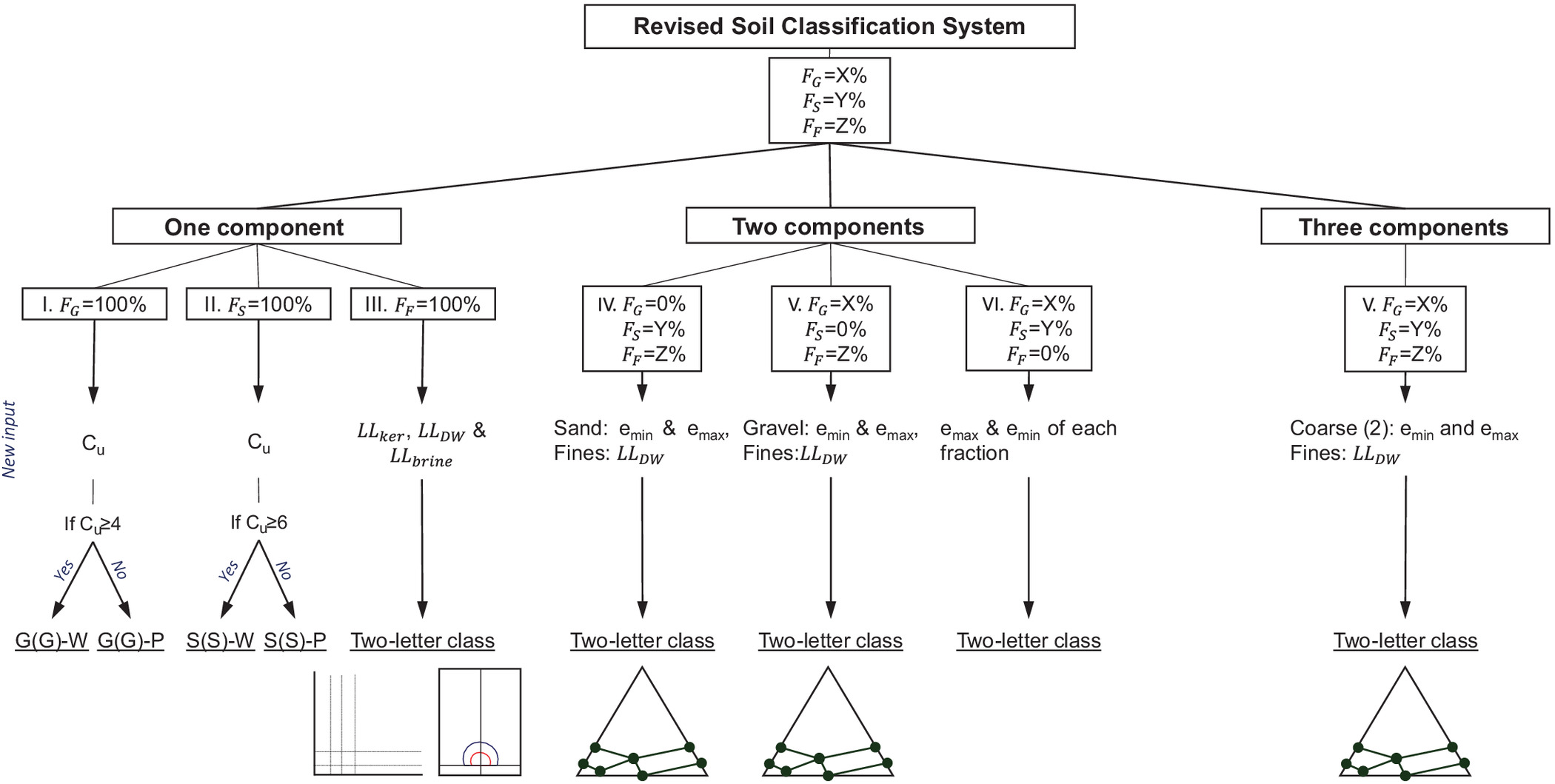
Fig. 4 shows the logic tree for the RSCS. It requires the mass fraction passing sieves #4 and #200 to identify gravel

F_{G}

(

> # 4

), sand

F_{S}

(

< # 4

;

> # 200

) and fines

F_{F}

(

< # 200

) fractions (Appendix I). Subsequent requests for input information depend on whether the soil is a single, binary, or ternary mixture. For example, for clean coarse soils, [i.e., G(G), GS(S), or S(S)], there is no need for liquid limit information, but the coefficient of uniformity

C_{u}

is needed to determine either well- or poorly- graded sand or gravel [Fig. 4, Procedures 1 and 2]. Conversely, if all the soil passes sieve #200 (

F_{F} = 100 %

), the RSCS will require the three liquid limits

{LL}_{DW}

,

{LL}_{brine}

, and

{LL}_{\ker}

to complete the fines classification [Fig. 4, Procedure 3].

Fig. 4. Revised Soil Classification System: Complete logic tree. This decision-making structure is implemented in an Excel sheet [available from Energy GeoEngineering Laboratory (EGEL) website] and the mobile application (available from the Android Play Store). If the classification involves F or (F), include the classification of fines (Column 3). If the classification is G(G) or S(S), include grading information (Columns 1 or 2).

Simplified Classification

The differentiation between sands and gravels is unnecessary in many applications. In such cases, the classification simplifies from a ternary triangular plot to a binary linear segment to distinguish coarse-controlled (

> 75 μm

) from fines-controlled (

< 75 μm

) soils. The simplified classification requires only three input parameters: (1) fines fraction

F_{F}

, i.e., the mass of fines passing sieve #200 divided by the total mass (%); (2) the liquid limit of fines obtained with deionized water

{LL}_{DW}

; and (3) the

e^{\max}

and

e^{\min}

values of the coarse fraction retained on sieve #200 [Fig. 5(a)].

Fig. 5. Simplified RSCS. This simpler classification may suffice when there is no need to distinguish sands from gravels: (a) logic tree; and (b) triangular chart as a linear plot.

The only three notable mixtures in this case define

F_{F} |^{H}

,

F_{F} |^{L}

and

F_{F} |^{flow}

, and correspond to Points 4, 8, and 13 in Fig. 2 and Appendix III. Fig. 5(b) shows the simplified classification for coarse C and fines F mixtures. The simplified classification results in four soil groups to recognize mechanical and fluid flow control: C(C), C(F), CF(F), and F(F). Clearly, when mixtures are fines-controlled, the classification still requires the three liquid limits to classify the fines:

{LL}_{DW}

,

{LL}_{brine}

, and

{LL}_{\ker}

. The simplified classification reduces the number of required tests and expedites the entire classification without losing physical meaning.

Reference Effective Stress for Fines: Soft and Stiff

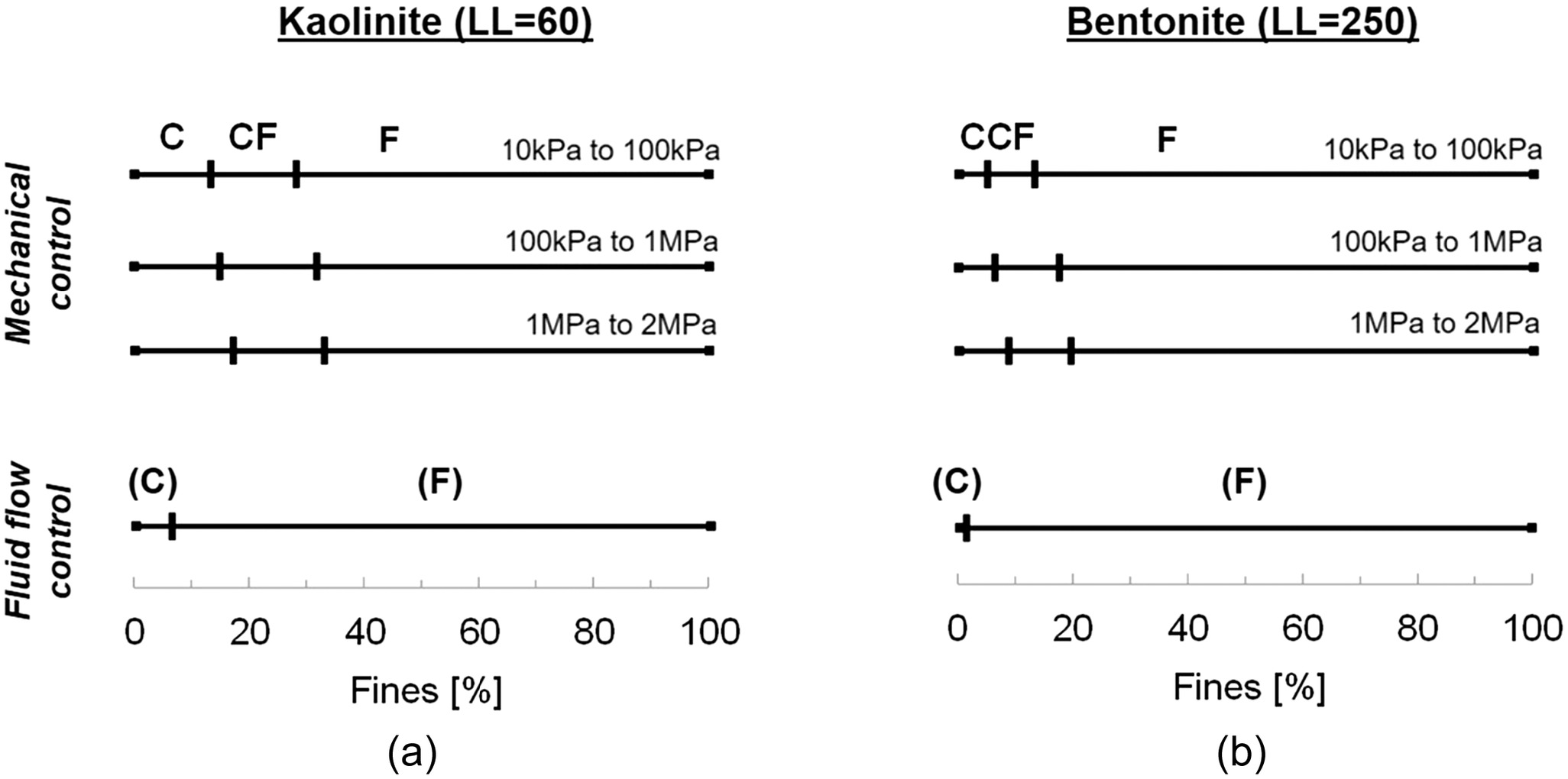
The two reference void ratios for soft (

e_{F} |^{10 kPa}

and stiff (

e_{F} |^{1 MPa}

) fines reflect common stress conditions in near-surface engineering applications (Appendix II). However, an initially load-carrying fine-grained matrix compacts and may give rise to a coarse-grained load-carrying skeleton at higher stress levels relevant to other applications. For example, the analysist may choose

e_{F} |^{100 kPa}

and

e_{F} |^{10 MPa}

for reservoir engineering, or

e_{F} |^{1 kPa}

and

e_{F} |^{100 kPa}

for near-seafloor offshore engineering projects. Implications can be analyzed readily within the RSCS [Fig. 6 (refer to Appendix II)]; flow boundaries are based on suspension viscosity and are not adjusted for stress level. Preliminary results obtained for kaolinite and bentonite show that higher stress levels shift boundaries to higher thresholds, but changes have a relatively minor effect for classification purposes (Fig. 6).

Fig. 6. Modification to accommodate different stress regimes. Threshold fractions for mechanical control computed for stress levels of 10–100 kPa, 100 kPa–1 MPa, and 1–2 MPa: (a) kaolinite–sand mixture; and (b) bentonite–sand mixture. The coarse fraction assumed for this analysis has $e^{\max} = 0.69$ and $e^{\min} = 0.40$ . As a first-order approximation, fluid flow boundaries remain unaffected by changes in the stress level. For clarity, this analysis was conducted for the simplified RSCS (refer to Fig. 5).

User-Friendly Excel Macro and Mobile App

We developed a user-friendly Excel sheet and a mobile application to facilitate the implementation of the RSCS (Fig. S2). The Excel sheet for the RSCS is available on the Energy GeoEngineering Laboratory website 2021, and the mobile app is available in the Android Play Store. Both the mobile app and the Excel sheet draw all RSCS charts, identify classification boundaries, and plot the point that represents the soil under consideration. The user-friendly software is organized into three main zones: input box, soil-specific triangular chart, and fines classification chart with electrical sensitivity criteria.

The RSCS adopts the threshold fines fraction for fluid flow

e_{F} |^{flow} = λ \cdot e_{F} |^{LL}

where

λ = [2 \log (LL - 25)]

(Appendix II). When the liquid limit of fines is

LL < 25

, the plasticity-dependent parameter is

λ = 1

, and the flow-control boundary is identical to the mechanical control boundary for clean coarse grains. As a result, the chart for soils with low-plasticity fines

LL < 25

does not have G(F), GS(F), and S(F) soil groups.

Both the Excel sheet and the mobile app report the two-letter group name to identify the load-carrying fraction(s) and the flow-controlling fraction. If the soil group includes either F for load-carrying fines or (F) for fines-controlled flow, the classification adds information about the fines plasticity and electrical sensitivity. For example, in S(F)–HI soil

•

S indicates that sand controls the mechanical response;

•

(F) indicates that fines control fluid flow; and

•

HI indicates that fines exhibit high plasticity and intermediate electrical sensitivity

We encourage users to report all input parameters, the soil classification, and the soil-specific classification charts in technical documents and publications.

Sediment Properties

The RSCS is more involved than previous classifications such as the Unified Soil Classification System. However, its implementation using the Excel sheet or the mobile app actually is simpler than the USCS. Most importantly, the RSCS is much more informative and predictive of the soil physical properties.

Ongoing and published studies have begun to show the RSCS guiding capabilities in various applications: experimental data analyses, specimen characterization, critical fines content, methane hydrate pore habit, polymer bonding, clogging, bioactivity in soils, geoacoustic properties, pore-fluid chemistry effects in fine-grained sediments, compressibility, cyclic behavior, desiccation cracks, and fluid flow in porous media (e.g., Cao 2017; Eslami et al. 2018; Lei and Santamarina 2018; Cao et al. 2019; Ekici et al. 2019; Jang et al. 2019; Lei et al. 2019; Bachus et al. 2019; Shivaram 2019; Jarrar et al. 2020; Wang et al. 2020; Terzariol et al. 2020; Vitone et al. 2019; Zhao and Santamarina 2020).

This section explores the transition from coarse-controlled to fines-controlled soil properties. We superimposed RSCS and USCS boundaries on each data set to compare the two classification systems.

Mechanical: Compressibility

Fig. 7(a) presents compression index

C_{c}

and swelling index

C_{s}

data for sand–kaolin mixtures versus the fines fraction

F_{F}

. Kaolin is an intermediate plasticity and intermediate electrical sensitivity fine-grained soil “II” based on the RSCS. RSCS boundaries properly divide the mixture compressibility into the three categories: (1) coarse-controlled, (2) transitional, and (3) fines-controlled. In comparison, the USCS considers the transitional clayey sand zone to be wider than the observed response (see similar data in Carrera et al. 2011; Simpson and Evans 2015).

Fig. 7. Mechanical and fluid flow soil properties—trends and classification: (a) compressibility for sand–kaolinite mixtures (silica sand from Jeddah, Saudi Arabia: $e_{C}^{\max} = 0.81$ , $e_{C}^{\min} = 0.45$ ; RP2 kaolinite from Gordon: ${LL}_{DW} = 67$ ) (data from Cordero et al. 2017); (b) residual shear strength in terms of $\tan ϕ$ for sand–bentonite mixtures (Toyoura sand: $e_{C}^{\max} = 0.95$ , $e_{C}^{\min} = 0.72$ ; bentonite: $LL = 250$ ) (data from Tiwari and Marui 2005); (c) hydraulic conductivity for gravel–sand mixture (5-mm glass beads: $e_{G}^{\max} = 0.72$ , $e_{G}^{\min} = 0.54$ ; Accusand: $e_{S}^{\max} = 0.74$ , $e_{S}^{\min} = 0.50$ ) (data from Zhang et al. 2011); and (d) hydraulic conductivity for gravel–fines mixtures (uniformly-graded gravel $d = 9 - 19 mm$ : $e_{G}^{\max} = 0.68$ , $e_{G}^{\min} = 0.44$ ; mine spoil from northeastern US: $LL = 37$ ) The RSCS classification results appear at the top of each plot. For comparison, figures include the USCS at the bottom (data from Shelley and Daniel 1993).

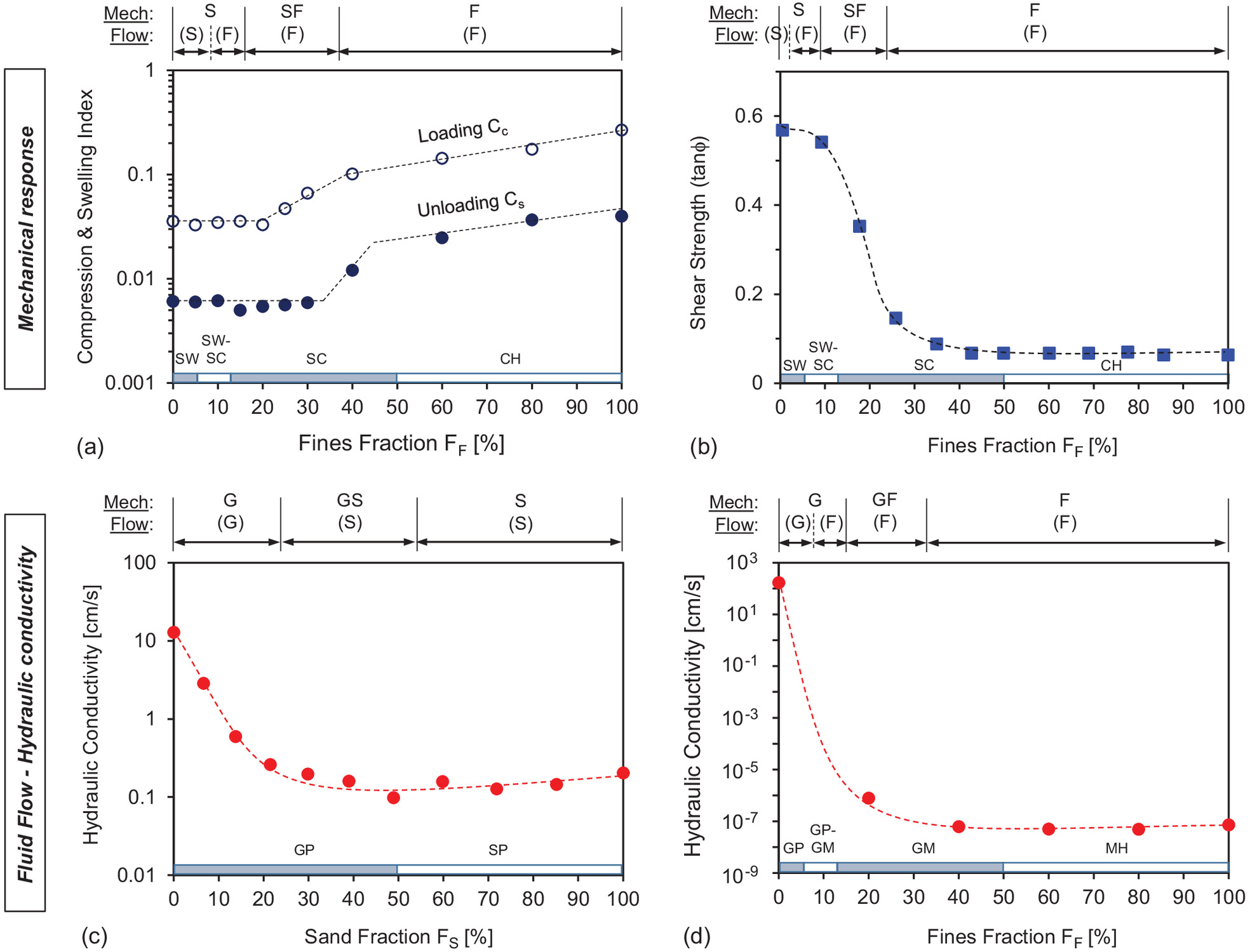
Mechanical: Shear Strength in Terms of tan φ

Fig. 7(b) plots the residual friction angle

\tan ϕ_{r}

against the fines fraction

F_{F}

based on measurements using the ring shear test with remolded specimens mixed with distilled water at an initial water content near the liquid limit before consolidation using a multistage ring shear. The mixture exhibits a significant decrease in

\tan ϕ_{r}

within the SF(F) group as it transitions from coarse- to fines-controlled shear strength. The transition falls within a much wider category in the USCS (see similar data for gravel–sand mixtures in Simoni and Houlsby 2006).

Fluid Flow: Hydraulic Conductivity

Fig. 7(c) plots the hydraulic conductivity

k

versus sand fraction

F_{S}

for gravel–sand mixtures. There is a dramatic reduction in hydraulic conductivity in the sand-controlled groups GS(S) and S(S). Fig. 7(d) illustrates the hydraulic conductivity

k

versus fines fraction

F_{F}

for coarse–fine mixtures; the RSCS captures the critical role of fines in permeability. By contrast, the USCS does not identify the soil fraction responsible for fluid flow.

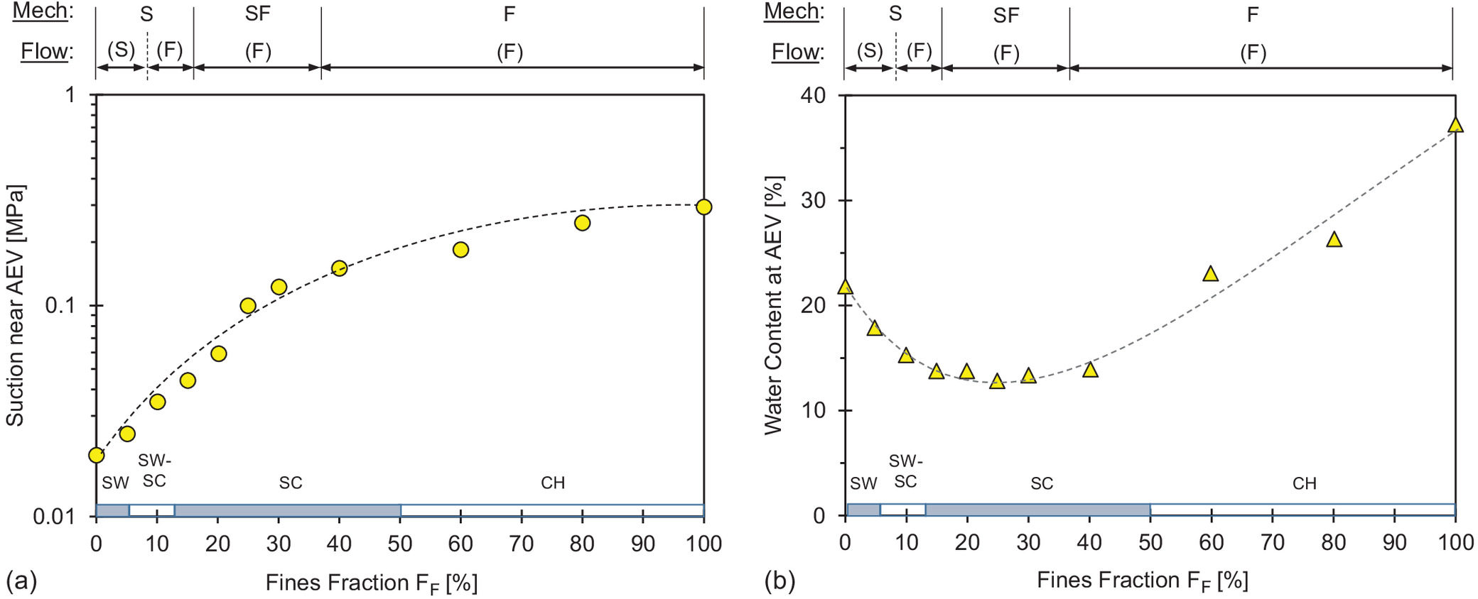
Unsaturated Soil: Suction Near AEV

Fig. 8(a) shows the effect of pore-size reduction caused by the addition of kaolinite to sand on the magnitude of suction near the air-entry value (AEV). The 11 sand–kaolinite specimens were mixed homogenously with deionized water to form pastes near the liquid limit. Specimens then were tested using a dewpoint hygrometer device to determine the complete soil-water characteristic curve (WP4C PotentiaMeter, Meter Group, Pullman, Washington). For completeness, Fig. 8(b) presents the gravimetric water content at the air-entry value versus fines fraction

F_{F}

. The water content at the AEV for sand-controlled mixtures decreased with an increase in the clay fraction because clays fill pores and reduce the porosity at low fines fraction. However, the gravimetric water content at the AEV increased because the kaolinite controls the pore size at high fines fractions. The effect of fines on the gravimetric water content at the AEV is more remarkable when higher plasticity clays are involved (Cordero et al. 2017). The RSCS boundaries superimposed on Figs. 8(a and b) properly anticipate transitions in capillary phenomena.

Fig. 8. Unsaturated soils—capillary phenomena: (a) suction at the AEV versus fines fraction; and (b) water content at AEV versus fines fraction. Figures include the RSCS at the top and the USCS at the bottom. Soil mixtures included silica sand from Jeddah, Saudi Arabia ( $e_{C}^{\max} = 0.81$ , $e_{C}^{\min} = 0.45$ ) and RP2 kaolinite from Gordon ( ${LL}_{DW} = 67$ ). (Data from Cordero et al. 2017.)

Other Engineering Properties

As part of this study, we compiled data sets to explore other engineering properties as a function of fines fraction. We determined the RSCS boundaries using soil characteristics provided in each case (Figs. S3–S12). Classification results clearly identify the transition from fines- to coarse-controlled behavior in mechanical and fluid flow transport properties. Engineering soil properties compiled from the literature include critical state parameters

M

and

Γ

[Figs. S3 and S4 (Marto et al. 2014; Carrera et al. 2011)], thermal conductivity [Fig. S5 (Yun et al. 2007; Roshankhah et al. 2021)], geophysical properties such as P- and S-wave velocities and electrical conductivity [Figs. S6–S8 (Kang and Lee 2015)], compression index [Fig. S9 (Carrera et al. 2011; Simpson and Evans 2015)], shear strength for gravel–sand mixtures [Fig. S10 (Simoni and Houlsby 2006)], and cyclic response [Fig. S11 (Law Engineering 1994)]. From the fines-classification point of view, a minor addition of biopolymers has a marked effect on the three liquid limits

{LL}_{DW}

,

{LL}_{brine}

, and

{LL}_{\ker}

[Fig. S12 (Chang et al. 2019)]. All data sets confirmed that the RSCS boundaries properly capture the coarse-controlled, transitional, and fines-controlled response in each case in addition to fines sensitivity to pore-fluid chemistry.

Engineering Relevance

This section explores other geotechnical phenomena and cases that demonstrate the predictive power and potential value of the revised classification RSCS.

Fines Migration

Internal instability refers to the seepage-induced fines migration through a load-carrying coarse granular skeleton (Moffat et al. 2011; Park et al. 2018). Fig. 9 plots internally stable and unstable soils reported in the literature in a generic triangular chart. The results show that clean coarse groups or soils in which the fines contents are insufficient to be load-carrying [e.g., GF(F), G(F), G(G), GS(S), S(F), S(S)] have a higher probability of undergoing seepage-induced internal instability. Given the wide range of soils reported in Fig. 9, the generic textural chart does not capture soil-specific classification boundaries, but it does facilitate clustering to anticipate internal instability below the green line.

Misclassification

Soil classification is a crucial preliminary step to guide the selection of soil engineering strategies. Consider soils at the Savannah River Site, South Carolina. We used the USCS and the RSCS to classify 99 soils gathered at two sampling locations: Site 1 used data from Law Engineering (1994), and Site 2 used data from Shannon and Wilson 2007 (Figs. 10 and S11). The USCS classifies most of the sediments as sands with some silt and clay (Fig. 10). In contrast, the RSCS anticipates that the fines fraction controls fluid flow in all specimens, and the mechanical properties in most cases [except for soils made of angular coarse particles with low plasticity fines (Fig. 10)].

The controlling role of fines was confirmed subsequently through extensive laboratory studies. Fig. S11 displays results from low-amplitude cyclic loading tests performed on soils from the Savannah River Site; the RSCS clearly separates fines-dominant mixtures F(F) from transitional mixtures SF(F), and shows that fines-dominant soils generate a lower pore pressure ratio than transitional mixtures at all shear strain levels. In comparison, the USCS fails to relate the soil response to its composition—compare Fig. S11(a) generated with the RSCS and Fig. 11(b) generated using the USCS.

Bioactivity

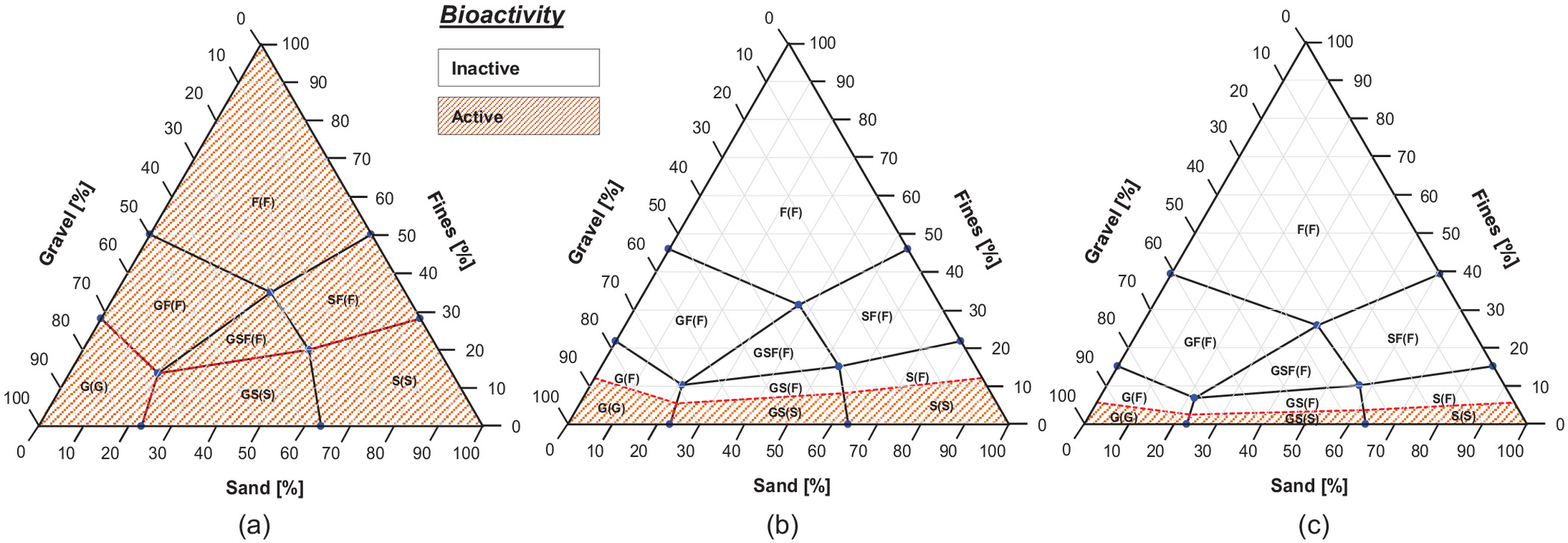
The pore size is a critical limiting factor for bioactivity in soils (Mitchell and Santamarina 2005; Rebata-Landa and Santamarina 2006), and it determines depth-dependent microbial cell counts in deep sediments (Park and Santamarina 2020). The void ratio of fines at the liquid limit with deionized water

e_{F} |^{LL} = G_{s} \cdot LL / 100

and the correlation between the specific surface

S_{s}

and liquid limit

S_{s} = 1.8 m^{2} / g \cdot LL 34 m^{2} / g

(Farrar and Coleman 1967) allows us to estimate the mean pore size

d_{pore}

in a soil as a function of its liquid limit (Phadnis and Santamarina 2011)

d_{pore} = \frac{k \cdot e_{F} |^{LL}}{S_{s} ρ_{m}} = \frac{LL}{25 (1.8 m^{2} / g LL 34 m^{2} / g) ρ_{m}} (where k = 4)

(1)

where

ρ_{m} = ρ_{w} G_{s}

= mineral density, where

G_{s}

= specific gravity of grains; and

k

= structure factor that depends on grain shape and sediment structure (

k \approx 2 - 4

). This simple equation implies that a sediment mixture in which a kaolinite (

LL = 60

,

S_{s} = 20 m^{2} / g

,

ρ_{m} = 10^{6} g / m^{3}

, and

k = 3

) fills the pores between coarse grains has a mean pore size

μ_{d} = 0.09 μm

and cannot accommodate biological activity. Therefore, we can anticipate biologically inactive groups in the RSCS. Bioactivity is hindered in the white zones in Fig. 11, in which plastic fines determine the pore size; conversely, bioactivity can flourish in soils that fall within the red hatched zones, i.e., silts or clean coarse soils.

This first-order analysis [Eq. (1)] assumes that the fines fraction is at the liquid limit and disregards the consolidation caused by the overburden pressure. In fact, cell counts decrease with depth (Parkes et al. 1994; Jørgensen and D’Hondt 2006). A detailed analysis involves soil compressibility, specific surface area, and pore-size distribution to properly anticipate depth-dependent microbial activity in sediments (Park and Santamarina 2020). The goal is to estimate the probability of pores size

d

being larger than the nominal microbe size

\approx 1 μm

; the analysis showed that

P (d \geq 1 μm) = 1.0

in silt and sand,

10^{- 2} - 10^{- 5}

in kaolinite,

10^{- 3} - 10^{- 10}

in illite, and

10^{- 5} - 10^{- 12}

in montmorillonite (the ranges reflect near-surface to

\sim 1,000 - m

burial depth). Therefore, pore size is not a limiting factor in coarse-dominant mixtures [Fig. 11(a)], but bioactivity will diminish as the plasticity of fines increases [Figs. 11(b and c)].

Soil Improvement

The selection of soil improvement techniques must recognize the hydraulic and mechanical soil response. Therefore, the RSCS can help preselect potential soil improvement techniques; for example (based on Mitchell 1981), F(F) soils are best treated by preloading with wick drains, whereas clean sands and gravels G(G), GS(S), and S(S) can be treated by deep dynamic compaction, vibrocompaction, or even permeation grouting if the gravel fraction controls G(G). Fluid flow in transitional soils GF(F), GSF(F), and SF(F) is always fines controlled, but they may exhibit low compressibility; in this case, jet grouting may be most advantageous.

Conclusions

Soil classification systems aim to help geotechnical engineers anticipate soil properties and guide the preliminary selection of geotechnical solutions. The physics-informed and data-driven Revised Soil Classification System groups soils into similar response categories based on soil index properties and adopts soil-specific classification boundaries (rather than the fixed 50%-passing boundaries in the USCS). This study clarifies the implementation of the RSCS, provides supportive evidence, and addresses relevant engineering implications. Salient conclusions are as follows:

•

The RSCS recognizes the pronounced effect of the fines fraction and its plasticity on mechanical and fluid flow properties, the role of particle shape on coarse-grain packing, and the relevance of pore-fluid chemistry in the behavior of fines.

•

Differences between the RSCS and USCS become more apparent for sediments that involve highly plastic fines and rounded coarse particles. Extensive databases show enhanced predictive clustering in the RSCS.

•

The RSCS can be adapted readily to address context-dependent conditions; in particular, it can accommodate different stress regimes and pore-fluid chemistries that are relevant to specific field situations.

•

When the coarse fraction does not need to be divided into sand and gravel fractions for a specific application, the RSCS can be simplified without loss of physical insight.

•

The RSCS adequately captures the transition from coarse-controlled to fines-controlled behavior in soil properties, including small strain stiffness and shear wave velocity, compressibility, shear strength and critical state parameters, response to repetitive loading, hydraulic conductivity, capillarity-saturation response, electrical conductivity, bioactivity, and sensitivity to pore-fluid chemistry.

•

Clearly, the RSCS provides a more informative soil classification in view of soil properties and preliminary engineering choices. Its implementation is facilitated by a freely available mobile app and Excel sheet.

•

The classification is based on index tests conducted with remolded samples. Therefore, diagenetic effects such as cementation are not captured by the RSCS, and require complementary in situ testing to enhance the preliminary characterization of the subsurface.

•

We encourage the community to document index properties and both current soil classifications and the RSCS in future reports and manuscripts. Ensuing databases will help future researchers develop better tools to advance geotechnical engineering further.

Supplemental Materials

File (supplemental_materials_jggefk.gteng-10447_castro.pdf)

Download
1.37 MB

Appendix I. Revised Soil Classification System—Necessary Input

Soil under consideration		Necessary input for RSCS boundary generation		Threshold fraction
Soil type	Definition	Void ratio	Index property	Threshold fraction
Gravel $G$ ( $> 4.75 mm$ )	$F_{G} = M_{G} / M_{T}$	$e_{G}^{\max}$ and $e_{G}^{\min}$	or $R$ and $C_{u}$	$F_{G} = \frac{1}{(1 + \frac{e_{G}}{1 + e_{S}} + \frac{e_{S}}{1 + e_{F}} \frac{e_{G}}{1 + e_{S}})}$
Sand $S$ ( $0.075 - 4.75 mm$ )	$F_{S} = M_{S} / M_{T}$	$e_{S}^{\max}$ and $e_{S}^{\min}$	or $R$ and $C_{u}$	$F_{S} = \frac{1}{(\frac{1 + e_{S}}{e_{G}} + 1 + \frac{e_{S}}{1 + e_{F}})}$
Fines $F$ ( $< 0.075 mm$ )	$F_{F} = M_{F} / M_{T}$	$e_{F} \|^{10 kPa}$ , $e_{F} \|^{1 MPa}$ , $e_{F} \|^{LL}$	or LL	$F_{F} = \frac{1}{(\frac{1 + e_{S}}{e_{G}} \frac{1 + e_{F}}{e_{S}} + \frac{1 + e_{F}}{e_{S}} + 1)}$

Appendix II. Revised Soil Classification System—Correlations

Process	Soil fraction(s)	Correlations
Load carrying	Gravel and sand: load-carrying	$e_{C}^{\max} = 0.032 + \frac{0.154}{R} + \frac{0.522}{C_{u}}$
		$e_{C}^{\min} = - 0.012 + \frac{0.082}{R} + \frac{0.371}{C_{u}}$
		(Youd 1973; Cho et al. 2006)
	Fines: load-carrying	${e_{F} \|}^{10 kPa} = {e_{F} \|}^{1 kPa} - C_{c} = 0.026 LL + 0.07$
		${e_{F} \|}^{1 MPa} = {e_{F} \|}^{1 kPa} - 3 C_{c} = 0.011 LL + 0.21$
		(Chong and Santamarina 2016)
Fluid flow	Fines: fluid flow	${e_{F} \|}^{flow} = λ \cdot {e_{F} \|}^{LL} = [2 \log (LL - 25)] \cdot {e_{F} \|}^{LL} \approx 0.05 LL \cdot \log (LL - 25) (λ \geq 1)$
Fluid flow	Fines: fluid flow	(Park and Santamarina 2017)

Appendix III. Revised Soil Classification System Boundaries—Notable Mixtures

Process	Controlling fraction	Mixture no.	Notable mixtures—packing condition
Process	Controlling fraction	Mixture no.	Gravel	Sand	Fines
Load-carrying	Gravel-controlled	1	$e_{G}^{\min}$	—	$e_{F} \|^{10 kPa}$
		2	$e_{G}^{\min}$	$e_{S}^{\max}$	—
		3	$e_{G}^{\min}$	$e_{S}^{\max}$	$e_{F} \|^{10 kPa}$
	Sand-controlled	4	—	$e_{S}^{\min}$	$e_{F} \|^{10 kPa}$
		5	$2.5 e_{G}^{\max}$	$e_{S}^{\min}$	—
		6	$2.5 e_{G}^{\max}$	$e_{S}^{\min}$	$e_{F} \|^{10 kPa}$
	Fines-controlled	7	$1.3 e_{G}^{\max}$	—	$e_{F} \|^{1 MPa}$
		8	—	$1.3 e_{S}^{\max}$	$e_{F} \|^{1 MPa}$
		9	$2.5 e_{G}^{\max}$	$1.3 e_{S}^{\max}$	$e_{F} \|^{1 MPa}$
Fluid flow	Fines-controlled	10	$e_{G}^{\min}$	—	$λ e_{F} \|^{LL}$
		11	$e_{G}^{\min}$	$e_{S}^{\max}$	$λ e_{F} \|^{LL}$
		12	$2.5 e_{G}^{\max}$	$e_{S}^{\min}$	$λ e_{F} \|^{LL}$
		13	—	$e_{S}^{\min}$	$λ e_{F} \|^{LL}$

Appendix IV. Fines Classification Based on Plasticity and Electrical Sensitivity

Input	Liquid limit ratios defined from input	Electrical sensitivity $S_{E}$ defined from liquid limit ratios
LL with deionized water ${LL}_{DW}$	${\frac{{LL}_{\ker}}{{LL}_{brine}} \|}_{corr} = \frac{{LL}_{\ker}}{{LL}_{brine}} \frac{1 - c_{brine} \frac{{LL}_{brine}}{100}}{G_{\ker}}$	Left: ${LL}_{\ker} / {LL}_{brine} > 1$
		$S_{E} (left) = \sqrt{{(\frac{{LL}_{\ker}}{{LL}_{brine}} - 1)}^{2} + {(\frac{{LL}_{DW}}{{LL}_{brine}} - 1)}^{2}}$
		Right: ${LL}_{\ker} / {LL}_{brine} < 1$
	${\frac{{LL}_{DW}}{{LL}_{brine}} \|}_{corr} = \frac{{LL}_{DW}}{{LL}_{brine}} (1 - c_{brine} \frac{{LL}_{brine}}{100})$	$S_{E} (right) = \sqrt{{(\frac{{LL}_{brine}}{{LL}_{\ker}} - 1)}^{2} + {(\frac{{LL}_{DW}}{{LL}_{brine}} - 1)}^{2}}$
LL with 2-M brine ${LL}_{brine}$
LL with kerosene ${LL}_{\ker}$

Note: Left and right refer to the side in the x-axis on Fig. 3(a) with respect to a nonsensitive soil response (1).

Data Availability Statement

All data, models, and code generated or used during the study appear in the published article and its associated supplemental materials.

Acknowledgments

Support for this research was provided by the KAUST Endowment at King Abdullah University of Science and Technology. Gabrielle E. Abelskamp edited the manuscript.

References

Bachus, R. C., et al. 2019. “Characterization and engineering properties of dry and ponded Class-F fly ash.” J. Geotech. Geoenviron. Eng. 145 (3): 04019003. https://doi.org/10.1061/(ASCE)GT.1943-5606.0001986.

Google Scholar

Burenkova, V. V. 1993. “Assessment of suffusion in non-cohesive and graded soils.” In Filters in geotechnical and hydraulic engineering, 357–360. Rotterdam, Netherlands: A. A. Balkema.

Google Scholar

Burland, J. B. 1990. “On the compressibility and shear strength of natural clays.” Géotechnique 40 (3): 329–378. https://doi.org/10.1680/geot.1990.40.3.329.

Google Scholar

Burmister, D. M. 1951. In Vol. 1. of Soil mechanic. New York: Columbia Univ.

Google Scholar

Cao, S. 2017. Microfluidic pore model study on physical and geomechanical factors influencing fluid flow behavior in porous media. Baton Rouge, LA: Louisiana State Univ.

Google Scholar

Cao, S. C., J. Jang, J. Jung, W. F. Waite, T. S. Collett, and P. Kumar. 2019. “2D micromodel study of clogging behavior of fine-grained particles associated with gas hydrate production in NGHP-02 gas hydrate reservoir sediments.” Mar. Pet. Geol. 108 (Oct): 714–730. https://doi.org/10.1016/j.marpetgeo.2018.09.010.

Google Scholar

Carrera, A., M. Coop, and R. Lancellotta. 2011. “Influence of grading on the mechanical behavior of Stava tailings.” Géotechnique 61 (11): 935–946. https://doi.org/10.1680/geot.9.P.009.

Google Scholar

Casagrande, A. 1948. “Classification and identification of soils.” Trans. ASCE 113 (1): 901–930. https://doi.org/10.1061/TACEAT.0006109.

Google Scholar

Chang, I., Y. M. Kwon, J. Im, and G. C. Cho. 2019. “Soil consistency and interparticle characteristics of xanthan gum biopolymer–containing soils with pore-fluid variation.” Can. Geotech. J. 56 (8): 1206–1213. https://doi.org/10.1139/cgj-2018-0254.

Google Scholar

Chapuis, R. P., A. Contant, and K. A. Baass. 1996. “Migration of fines in 0–20 mm crushed base during placement, compaction, and seepage under laboratory conditions.” Can. Geotech. J. 33 (1): 168–176. https://doi.org/10.1139/t96-032.

Google Scholar

Cho, G. C., J. Dodds, and J. C. Santamarina. 2006. “Particle shape effects on packing density, stiffness, and strength: Natural and crushed sands.” J. Geotech. Geoenviron. Eng. 132 (5): 591–602. https://doi.org/10.1061/(ASCE)1090-0241(2006)132:5(591).

Google Scholar

Chong, S. H., and J. C. Santamarina. 2016. “Soil compressibility models for a wide stress range.” J. Geotech. Geoenviron. Eng. 142 (6): 06016003. https://doi.org/10.1061/(ASCE)GT.1943-5606.0001482.

Google Scholar

Cordero, J. A., G. Useche, P. C. Prat, A. Ledesma, and J. C. Santamarina. 2017. “Soil desiccation cracks as a suction–contraction process.” Géotech. Lett. 7 (4): 279–285. https://doi.org/10.1680/jgele.17.00070.

Google Scholar

Ekici, A., N. Huvaj, and C. Akgüner. 2019. “Index properties and classification of marginal fills or coarse-fine mixtures.” In Proc., Geo-Congress 2019: Engineering Geology, Site Characterization, and Geophysics, 91–99. Reston, VA: ASCE.

Google Scholar

Eslami, M. M., S. J. Brandenberg, and J. P. Stewart. 2018. “Cyclic behavior of low-plasticity fine-grained soils with varying pore-fluid salinity.” In Geotechnical Earthquake Engineering and Soil Dynamics V: Slope Stability and Landslides, Laboratory Testing, and In Situ Testing, Geotechnical Special Publication 293, edited by S. J. Brandenberg and M. T. Manzari, 171–179. Reston, VA: ASCE.

Google Scholar

Farrar, D. M., and J. D. Coleman. 1967. “The correlation of surface area with other properties of nineteen British clay soils.” J. Soil Sci. 18 (1): 118–124. https://doi.org/10.1111/j.1365-2389.1967.tb01493.x.

Google Scholar

Fragaszy, R. J., J. Su, F. H. Siddiqi, and C. L. Ho. 1992. “Modeling strength of sandy gravel.” J. Geotech. Eng. 118 (6): 920–935. https://doi.org/10.1061/(ASCE)0733-9410(1992)118:6(920).

Google Scholar

Holtz, R. D., and W. D. Kovacs. 1981. An introduction to geotechnical engineering. Englewood Cliffs, NJ: Prentice-Hall.

Google Scholar

Howard, A. K. 1984. “The revised ASTM standard on the Unified Classification System.” Geotech. Test. J. 7 (4): 216–222. https://doi.org/10.1520/GTJ10505J.

Google Scholar

Jang, J., and J. C. Santamarina. 2016. “Fines classification based on sensitivity to pore-fluid chemistry.” J. Geotech. Geoenviron. Eng. 142 (4): 06015018. https://doi.org/10.1061/(ASCE)GT.1943-5606.0001420.

Google Scholar

Jang, J., and J. C. Santamarina. 2017. “Closure to ‘Fines classification based on sensitivity to pore-fluid chemistry’ by Junbong Jang and J. Carlos Santamarina.” J. Geotech. Geoenviron. Eng. 142 (4): 07017013. https://doi.org/10.1061/(ASCE)GT.1943-5606.0001694.

Google Scholar

Jang, J., W. F. Waite, L. A. Stern, T. S. Collett, and P. Kumar. 2019. “Physical property characteristics of gas hydrate-bearing reservoir and associated seal sediments collected during NGHP-02 in the Krishna-Godavari Basin, in the offshore of India.” Mar. Pet. Geol. 108 (Oct): 249–271. https://doi.org/10.1016/j.marpetgeo.2018.09.027.

Google Scholar

Jarrar, Z. A., R. I. Al-Raoush, J. A. Hannun, K. A. Alshibli, and J. Jung. 2020. “3D synchrotron computed tomography study on the influence of fines on gas driven fractures in Sandy Sediments.” Geomech. Energy Environ. 23 (Jul): 100105. https://doi.org/10.1016/j.gete.2018.11.001.

Google Scholar

Jørgensen, B. B., and S. D’Hondt. 2006. “A starving majority deep beneath the seafloor.” Science 314 (5801): 932–934. https://doi.org/10.1126/science.1133796.

Google Scholar

Kang, M., and J. S. Lee. 2015. “Evaluation of the freezing–thawing effect in sand–silt mixtures using elastic waves and electrical resistivity.” Cold Reg. Sci. Technol. 113 (May): 1–11. https://doi.org/10.1016/j.coldregions.2015.02.004.

Google Scholar

Kenney, T. C., and D. Lau. 1985. “Internal stability of granular filters.” Can. Geotech. J. 22 (2): 215–225. https://doi.org/10.1139/t85-029.

Google Scholar

Kenney, T. C., D. Lau, and G. Clute. 1983. Filter tests on 235mm diameter specimens of granular materials. Toronto: Univ. of Toronto.

Google Scholar

Kim, H. K., D. D. Cortes, and J. C. Santamarina. 2007. “Flow test: Particle-level and macroscale analyses.” ACI Mater. J. 104 (3): 323–327. https://doi.org/10.14359/18679.

Google Scholar

Kulhawy, F. H., and J. R. Chen. 2009. “Identification and description of soils containing very coarse fractions.” J. Geotech. Geoenviron. Eng. 135 (5): 635–646. https://doi.org/10.1061/(ASCE)1090-0241(2009)135:5(635).

Google Scholar

Lafleur, J., J. Mlynarek, and A. L. Rollin. 1989. “Filtration of broadly graded cohesionless soils.” J. Geotech. Eng. 115 (12): 1747–1769. https://doi.org/10.1061/(ASCE)0733-9410(1989)115:12(1747).

Google Scholar

Law Engineering. 1994. Final report for ITP geotechnical services, 325. Aiken, SC: Westinghouse Savannah River Company.

Google Scholar

Lei, L., Z. Liu, Y. Seol, R. Boswell, and S. Dai. 2019. “An investigation of hydrate formation in unsaturated sediments using X-ray computed tomography.” J. Geophys. Res.: Solid Earth 124 (4): 3335–3349. https://doi.org/10.1029/2018JB016125.

Google Scholar

Lei, L., and J. C. Santamarina. 2018. “Laboratory strategies for hydrate formation in fine-grained sediments.” J. Geophys. Res.: Solid Earth 123 (4): 2583–2596. https://doi.org/10.1002/2017JB014624.

Google Scholar

Li, M. 2008. “Seepage induced instability in widely graded soils.” Ph.D. thesis, Dept. of Civil Engineering, Univ. of British Columbia.

Google Scholar

Marto, A., C. S. Tan, A. M. Makhtar, and T. Kung Leong. 2014. “Critical state of sand matrix soils.” Sci. World J. 2014 (Jan): 1–8. https://doi.org/10.1155/2014/290207.

Google Scholar

Mitchell, J. K. 1981. “Soil improvement: State-of-the-art.” In Vol. 4 of Proc., 10th Int. Conf. on Soil Mechanics and Foundation Engineering, 509–565. Stockholm, Sweden: International Society for Soil Mechanics and Geotechnical Engineering.

Google Scholar

Mitchell, J. K., and J. C. Santamarina. 2005. “Biological considerations in geotechnical engineering.” J. Geotech. Geoenviron. Eng. 131 (10): 1222–1233. https://doi.org/10.1061/(ASCE)1090-0241(2005)131:10(1222).

Google Scholar

Mitchell, J. K., and K. Soga. 2005. Fundamentals of soil behavior. 3rd ed. Hoboken, NJ: Wiley.

Google Scholar

Moffat, R., R. J. Fannin, and S. J. Garner. 2011. “Spatial and temporal progression of internal erosion in cohesionless soil.” Can. Geotech. J. 48 (3): 399–412. https://doi.org/10.1139/T10-071.

Google Scholar

Narsilio, G. A., M. M. Disfani, and A. Orangi. 2017. “Discussion of ‘Fines classification based on sensitivity to pore-fluid chemistry’ by Junbong Jang and J. Carlos Santamarina.” J. Geotech. Geoenviron. Eng. 143 (7): 07017009. https://doi.org/10.1061/(ASCE)GT.1943-5606.0001690.

Google Scholar

Park, J., G. M. Castro, and J. C. Santamarina. 2018. “Closure to ‘Revised soil classification system for coarse-fine mixtures’ by Junghee Park and J. Carlos Santamarina.” J. Geotech. Geoenviron. Eng. 144 (8): 07018019. https://doi.org/10.1061/(ASCE)GT.1943-5606.0001908.

Google Scholar

Park, J., and J. C. Santamarina. 2017. “Revised soil classification system for coarse-fine mixtures.” J. Geotech. Geoenviron. Eng. 143 (8): 04017039. https://doi.org/10.1061/(ASCE)GT.1943-5606.0001705.

Google Scholar

Park, J., and J. C. Santamarina. 2020. “The critical role of pore size on depth-dependent microbial cell counts in sediments.” Sci. Rep. 10 (1): 21692. https://doi.org/10.1038/s41598-020-78714-3.

Google Scholar

Parkes, R. J., B. A. Cragg, S. J. Bale, J. M. Getlifff, K. Goodman, P. A. Rochelle, J. C. Fry, A. J. Weightman, and S. M. Harvey. 1994. “Deep bacterial biosphere in Pacific Ocean sediments.” Nature 371 (6496): 410–413. https://doi.org/10.1038/371410a0.

Google Scholar

Phadnis, H. S., and J. C. Santamarina. 2011. “Bacteria in sediments: Pore size effects.” Géotech. Lett. 1 (4): 91–93. https://doi.org/10.1680/geolett.11.00008.

Google Scholar

Rebata-Landa, V., and J. C. Santamarina. 2006. “Mechanical limits to microbial activity in deep sediments.” Geochem. Geophys. Geosyst. 7 (11): 11006. https://doi.org/10.1029/2006GC001355.

Google Scholar

Roshankhah, S., A. V. Garcia, and J. C. Santamarina. 2021. “Thermal conductivity of sand–silt mixtures.” J. Geotech. Geoenviron. Eng. 147 (2): 06020031. https://doi.org/10.1061/(ASCE)GT.1943-5606.0002425.

Google Scholar

Santamarina, J. C. 2003. “Soil behavior at the microscale: Particle forces.” In Soil behavior and soft ground construction, 25–56. Reston, VA: ASCE.

Crossref

Google Scholar

Santamarina, J. C., K. A. Klein, and M. A. Fam. 2001. Soils and waves. New York: Wiley.

Google Scholar

Santamarina, J. C., K. A. Klein, A. Palomino, and M. S. Guimaraes. 2002. Micro-scale aspects of chemical-mechanical coupling—Interparticle forces and fabric, Maratea, 47–64. Rotterdam, Netherlands: A. A. Balkema.

Google Scholar

Shannon and Wilson. 2007. Geotechnical engineering report–Geotechnical investigation Phase II: Salt waste processing facility, 1945. Washington, DC: DOE.

Google Scholar

Shelley, T. L., and D. E. Daniel. 1993. “Effect of gravel on hydraulic conductivity of compacted soil liners.” J. Geotech. Engrg. 119 (1): 54–68. https://doi.org/10.1061/(ASCE)0733-9410(1993)119:1(54).

Google Scholar

Shivaram, K. K. 2019. “Radio-mediated polymeric bonding of soils.” Doctoral dissertation, Dept. of Civil Engineering, San Diego State Univ.

Google Scholar

Simoni, A., and G. T. Houlsby. 2006. “The direct shear strength and dilatancy of sand–gravel mixtures.” Geotech. Geol. Eng. 24 (3): 523–549. https://doi.org/10.1007/s10706-004-5832-6.

Google Scholar

Simpson, D. C., and T. M. Evans. 2015. “Behavioral thresholds in mixtures of sand and kaolinite clay.” J. Geotech. Geoenviron. Eng. 142 (2): 04015073. https://doi.org/10.1061/(ASCE)GT.1943-5606.0001391.

Google Scholar

Skempton, A. W. 1970. “The consolidation of clays by gravitational compaction.” Q. J. Geol. Soc. 125 (1–4): 373–411. https://doi.org/10.1144/gsjgs.125.1.0373.

Google Scholar

Skempton, A. W., and J. M. Brogan. 1994. “Experiments on piping in sandy gravels.” Géotechnique 44 (3): 449–460. https://doi.org/10.1680/geot.1994.44.3.449.

Google Scholar

Skempton, A. W., and O. T. Jones. 1944. “Notes on the compressibility of clays.” Q. J. Geol. Soc. 100 (1–4): 119–135. https://doi.org/10.1144/GSL.JGS.1944.100.01-04.08.

Google Scholar

Sun, B. C. 1989. “Internal stability of clayey to silty sands.” Ph.D. thesis, Dept. of Civil Engineering, Univ. of Michigan.

Google Scholar

Terzariol, M., J. Park, G. M. Castro, and J. C. Santamarina. 2020. “Methane hydrate-bearing sediments: Pore habit and implications.” Mar. Pet. Geol. 116 (Jun): 104302. https://doi.org/10.1016/j.marpetgeo.2020.104302.

Google Scholar

Tiwari, B., and H. Marui. 2005. “A new method for the correlation of residual shear strength of the soil with mineralogical composition.” J. Geotech. Geoenviron. Eng. 131 (9): 1139–1150. https://doi.org/10.1061/(ASCE)1090-0241(2005)131:9(1139).

Google Scholar

Vallejo, L. E. 2001. “Interpretation of the limits in shear strength in binary granular mixtures.” Can. Geotech. J. 38 (5): 1097–1104. https://doi.org/10.1139/t01-029.

Google Scholar

Vallejo, L. E., and R. Mawby. 2000. “Porosity influence on the shear strength of granular material–clay mixtures.” Eng. Geol. 58 (2): 125–136. https://doi.org/10.1016/S0013-7952(00)00051-X.

Google Scholar

Vitone, C., F. Sollecito, and F. Todaro. 2019. “Contaminated marine sites: Geotechnical issues bridging the gap between characterization and remedial strategies.” Riv. Ital. Geotecnica 4 (2020): 41–62. https://doi.org/10.19199/2020.4.0557-1405.041.

Google Scholar

Wagner, A. A. 1957. “The use of the unified soil classification system by the bureau of reclamation.” In Vol. 125 of Proc., 4th Int. Conf. on Soil Mechanics and Foundation Engineering, 125–134. London: International Society for Soil Mechanics and Geotechnical Engineering.

Google Scholar

Wan, C. F., and R. Fell. 2004. Experimental investigation of internal instability of soils in embankment dams and their foundations. Kensington, NSW, Australia: Univ. of New South Wales.

Google Scholar

Wang, L., Y. Li, P. Wu, S. Shen, T. Liu, S. Leng, Y. Chang, and J. Zhao. 2020. “Physical and mechanical properties of the overburden layer on gas hydrate-bearing sediments of the South China sea.” J. Pet. Sci. Eng. 189 (Jun): 107020. https://doi.org/10.1016/j.petrol.2020.107020.

Google Scholar

Youd, T. L. 1973. Factors controlling maximum and minimum densities of sands, 98–112. West Conshohocken, PA: ASTM.

Google Scholar

Yun, T. S., J. C. Santamarina, and C. Ruppel. 2007. “Mechanical properties of sand, silt, and clay containing tetrahydrofuran hydrate.” J. Geophys. Res.: Solid Earth 112 (4): B04106. https://doi.org/10.1029/2006JB004484.

Google Scholar

Zhang, Z. F., A. L. Ward, and J. M. Keller. 2011. “Determining the porosity and saturated hydraulic conductivity of binary mixtures.” Vadose Zone J. 10 (1): 313–321. https://doi.org/10.2136/vzj2009.0138.

Google Scholar

Zhao, B., and J. C. Santamarina. 2020. “Desiccation crack formation beneath the surface.” Géotechnique 70 (2): 181–186. https://doi.org/10.1680/jgeot.18.T.019.

Google Scholar

Information & Authors

Information

Published In

Journal of Geotechnical and Geoenvironmental Engineering

Volume 149 • Issue 11 • November 2023

Copyright

This work is made available under the terms of the Creative Commons Attribution 4.0 International license, https://creativecommons.org/licenses/by/4.0/.

History

Received: Oct 2, 2021

Accepted: Apr 25, 2023

Published online: Sep 13, 2023

Published in print: Nov 1, 2023

Discussion open until: Feb 13, 2024

Authors

Affiliations

Gloria M. Castro https://orcid.org/0000-0002-2667-1801

Formerly at KAUST, Teaching/Research Associate, Dept. of Civil and Environmental Engineering, Univ. of Strathclyde, Glasgow G1 1XJ, UK. ORCID: https://orcid.org/0000-0002-2667-1801

View all articles by this author

Junghee Park https://orcid.org/0000-0001-7033-4653 [email protected]

Formerly at KAUST, Assistant Professor, Dept. of Civil and Environmental Engineering, Incheon National Univ., 119 Academy-ro, Yeonsu-gu, Incheon 22012, Republic of Korea (corresponding author). ORCID: https://orcid.org/0000-0001-7033-4653. Email: [email protected]

View all articles by this author

J. Carlos Santamarina, A.M.ASCE https://orcid.org/0000-0001-8708-2827

Formerly at KAUST, Professor, School of Civil and Environmental Engineering, Georgia Institute of Technology, Atlanta, GA 30332. ORCID: https://orcid.org/0000-0001-8708-2827

View all articles by this author

Metrics & Citations

Metrics

Citations

Download citation

If you have the appropriate software installed, you can download article citation data to the citation manager of your choice. Simply select your manager software from the list below and click Download.

Abstract

Introduction

Fundamental Concepts Involved in the RSCS

Coarse–Fines Mixtures

Coarse Fraction

Fines Fraction

Fluid Transport Control Boundary

RSCS Boundaries

Comparison of RSCS and USCS

Fines Classification

Diagenesis

Implementation

Logic Tree: Decision-Making

Simplified Classification

Reference Effective Stress for Fines: Soft and Stiff

User-Friendly Excel Macro and Mobile App

Sediment Properties

Mechanical: Compressibility

Mechanical: Shear Strength in Terms of tan φ

Fluid Flow: Hydraulic Conductivity

Unsaturated Soil: Suction Near AEV

Other Engineering Properties

Engineering Relevance

Fines Migration

Misclassification

Bioactivity

Soil Improvement

Conclusions

Supplemental Materials

Appendix I. Revised Soil Classification System—Necessary Input

Appendix II. Revised Soil Classification System—Correlations

Appendix III. Revised Soil Classification System Boundaries—Notable Mixtures

Appendix IV. Fines Classification Based on Plasticity and Electrical Sensitivity

Data Availability Statement

Acknowledgments

References

Information

Published In

Copyright

History

ASCE Technical Topics:

Authors

Affiliations

Metrics

Citations

Download citation

Figures

Other

Share

Copy the content Link

Share with email

Share

Request Username

Create a new account

Change Password

Password Changed Successfully

Verify Phone

Congrats!