Investigation of Epoxy Resin under Uniaxial, Biaxial, and Triaxial Quasi-Static Loads
Publication: Journal of Engineering Mechanics
Volume 151, Issue 1
Abstract
Several studies indicate that epoxy resin exhibits a very wide range of mechanical behavior, in particular its strength, as a function of stress state. Especially when epoxy resin is used as matrix material for fiber reinforced composites (FRC), this becomes relevant due to complex stress conditions in the matrix. However, the knowledge about the behavior of epoxy resin under uni, bi, and triaxial stress conditions is lacking. Therefore, the mechanical properties of a typical epoxy resin for the production of FRC were investigated given such load conditions. The determined strengths were compared with the predictions of the extended paraboloid criterion. Uniaxial tension and compression tests, torsion tests with overlaid tension and compression, and triaxial tension tests were performed. An elastoplastic material model and a nonlocal damage model were formulated to demonstrate the application of the extended paraboloid strength criterion. In particular, large plastic strains under shear stress conditions, as well as a perfectly brittle material behavior with significantly reduced strength under triaxial tension, could be shown.
Introduction
In the field of continuous fiber reinforced polymers, micromechanical analyses have been established as a powerful tool for determining the effective properties of composites (Wan et al. 2023). To perform such analyses on composites, very accurate material models for the individual components are required (Morelle et al. 2017). In particular, highly crosslinked polymers such as epoxy resins are a frequently used matrix material for such high-performance composites.
Similar to all polymers, the mechanical behavior of epoxy shows both a time and a temperature dependence (Morelle et al. 2017; Poulain 2010; Gerlach et al. 2008; Littell et al. 2008; Wu et al. 2005; Werner and Daniel 2014) and a dependence on hydrostatic pressure (Fiedler et al. 2001b; Asp et al. 1995; Kim et al. 2013; Gross et al. 2017). Despite the high crosslinking density of the polymer chains, epoxy resins show similarities to the mechanical behavior of amorphous thermoplastics (Morelle et al. 2017) that in principle can be described by viscoelastic-viscoplastic material behavior (Nguyen et al. 2016).
Epoxy resins are used below their glass transition temperature in the glassy state. The material behavior is initially viscoelastic, with Young’s moduli in the range of 2–4 GPa and Poisson’s ratios between 0.3 and 0.4. Numerous investigations have shown that plastic flow begins after the viscoelastic part, which is particularly significant under compression and torsion (Fiedler et al. 2001b; Littell et al. 2008; Gerlach et al. 2008; Morelle et al. 2017). In contrast to thermoplastic materials, yield in epoxy resins cannot be explained by the slide of polymer chains due to the high crosslinking density. Molecular dynamics simulations indicate that the yield of epoxy resins is caused by a change in conformation through the rotation of chain segments (Sundararaghavan and Kumar 2013).
Under compression after reaching the first peak in the stress-strain curve, a decline in stress has been observed by some authors (Morelle et al. 2017; Littell et al. 2008). In other studies, this effect has been less prominent (Gerlach et al. 2008; Fiedler et al. 2001b; Werner and Daniel 2014). The cause of this softening effect has not yet been completely clarified. Morelle et al. (2017) attributed this effect to a large collective molecular movement. However, he admitted that the shape of the specimen and the test boundary conditions can lead to localization of the deformation in the form of necking/bellying and individual large shear bands.
This region is usually followed by a stress plateau with subsequent hardening, which is attributed to an increased orientation of the molecular network (Morelle et al. 2017). Under shear loads, ideal plastic behavior with very large deformations can be observed in epoxy resins (Littell et al. 2008; Fiedler et al. 2001b). Given increasing hydrostatic tension, the capacity for plastic deformation decreases. In the uniaxial tensile test, plastic deformation is less pronounced than it is under compression and shear (Morelle et al. 2017; Littell et al. 2008; Fiedler et al. 2001b; Gerlach et al. 2008). Under almost pure hydrostatic tension, plastic deformation can no longer be observed (Asp et al. 1995; Kim et al. 2013; Gross et al. 2017; Neogi et al. 2018).
Regardless of the preceding plastic deformation, brittle fracture mechanisms occur in epoxy resins when strength is reached (Fiedler et al. 2001b; Morelle et al. 2017). In this context, the strength of epoxy resins is also highly dependent on the existing hydrostatic pressure. In particular, under hydrostatic tension, a dramatic decrease in strength can be observed compared to the uniaxial tensile strength (Asp et al. 1995; Kim et al. 2013; Gross et al. 2017).
Various approaches to describing the strength of epoxy resins are based on the enlargement of cavities present in the material (Singh et al. 2017; Chevalier et al. 2019; Asp et al. 1996). Given increasing hydrostatic tensile content, the enlargement of such cavities in the resin increases (Neogi et al. 2018). This could be a reason for the low hydrostatic tensile strength of epoxy resin. In Roetsch and Horst (2022), a new strength criterion was developed as an extended form of the paraboloid criterion of Stassi-D’Alia (1967), which explicitly considers the hydrostatic tensile strengthwhere , , and represent the tensile, torsional, and hydrostatic strength of the material, respectively. Additionally, the first invariant of the stress tensor is defined (using Einstein’s summation convention)and the second invariant of the stress deviator where
(1)
(2)
(3)
(4)
(5)
(6)
(7)
When experimental values for the hydrostatic tensile strength are absent, the following is assumed (Roetsch and Horst 2022):
(8)
In this approach, = initial tensile yield stress; and = tensile strength of the material.
The aim of this work is to validate the extended paraboloid criterion using a typical epoxy resin for fiber composites as an example. For this purpose, the quasi-static strength under tensile, compressive, and torsional loading and under triaxial tension were determined. Furthermore, the application of the extended paraboloid criterion as a strength criterion is demonstrated in an elastoplastic material model with nonlinear damage. For this purpose, the elastoplastic material behavior under different loads was also investigated.
Experimental Investigation
Material and General Conditions
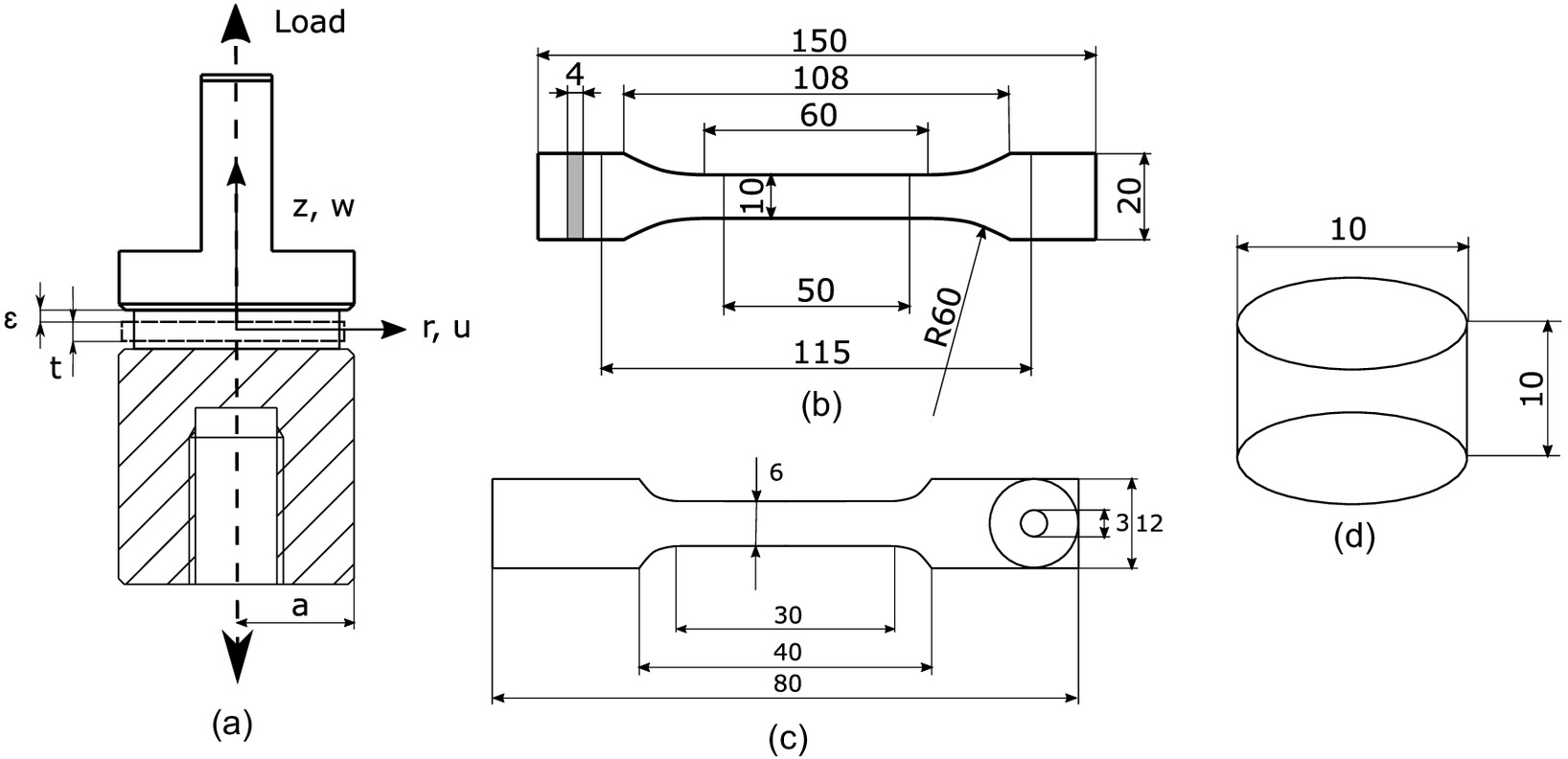
The epoxy investigated was a bisphenol-A/F-epichlorhydrin resin (Resin L) Supplier R&G Faserverbundwerkstoffe GmbH, Waldenbuch, Germany. The epoxy was processed with an isophorondiamin hardener (GL 1). Resin and hardener were carefully mixed for 5 min and vacuum processed for 2 min. The tensile specimens were cast in silicone molds. The compression and torsion specimens were first cast in a rod shape and then mechanically postprocessed. For the poker chip test, flat disc-shaped specimens were glued between steel rods. The manufacturing process for the poker chip specimens is described in detail in the “Poker Chip Test” section. The geometry of the test samples is shown in Fig. 1. To ensure a complete curing, different curing treatments were checked using tensile tests and differential scanning calorimetry (DSC) analysis:
•
,
•
, and
•
.
with C being the finally used curing cycle; see sections “DSC” & “Tensile Test.”
For all tests, a strain rate of was applied. The selected strain rate results as a compromise between the objective of quasi-static loading and moderate testing time. Furthermore, comparability with, for example, Fiedler et al. (2001a), Morelle et al. (2017), Gerlach et al. (2008), and Littell et al. (2008) was ensured. The tensile tests were performed using a universal test machine Zwick/Roell Z010 (ZwickRoell GmbH, Ulm, Germany) with a 10 kN load cell. The compression and poker-chip tests were done using a universal test machine Instron 4505 (Instron GmbH, Darmstadt, Germany) with a 100 kN load cell. The torsion tests were performed using a universal test machine Zwick/Roell Z250 (ZwickRoell GmbH) with a 250 kN load cell for axial loading and a 1,000 Nm torque sensor. For tension, compression, and poker chip test, at least 20 specimens were used. Due to the long testing time, five specimens were used for each of the torsion tests. Since all tests were performed under quasi-static conditions, elastoplastic material behavior was assumed. However, dynamic mechanical analysis (DMA) was carried out to estimate the proportion of viscoelastic material behavior (see section “DMA”).
Differential Scanning Calorimetry
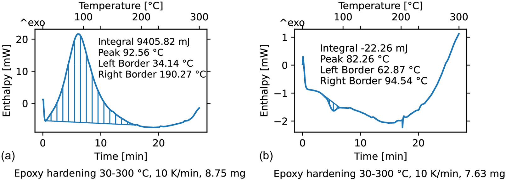
To ensure that the epoxy resin was completely cured, DSC analyses were performed to determine the degree of crosslinking. A Mettler Toledo type DSC 25 (Mettler Toledo, Columbus) heat flow differential calorimeter with a TC15 TA controller was used for the DSC analysis. Since the crosslinking process of epoxy resin is an exothermic reaction, the measured enthalpy of an uncured sample can be compared with that of a cured sample to draw conclusions on the degree of crosslinking of the epoxy resin. First, a freshly mixed sample was examined as a reference. The material was heated from room temperature to 300°C at a heating rate of . Fig. 2(a) shows the exotherm peak of the crosslink reaction. To evaluate the curing cycles, three epoxy resin samples were also heated from room temperature at to 300°C for each curing cycle. Fig. 2(b) shows the curve of the DSC measurement for a specimen produced with curing cycle C. The glass transition temperature range of the resin was between 70°C and 90°C. Since the curves for the remaining samples appeared very similar, they were not plotted. No further exothermic peak could be measured; therefore, complete crosslinking of the resin can be assumed.
Dynamic Mechanical Analysis
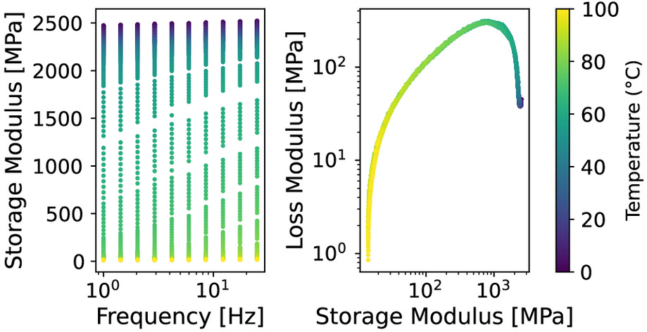
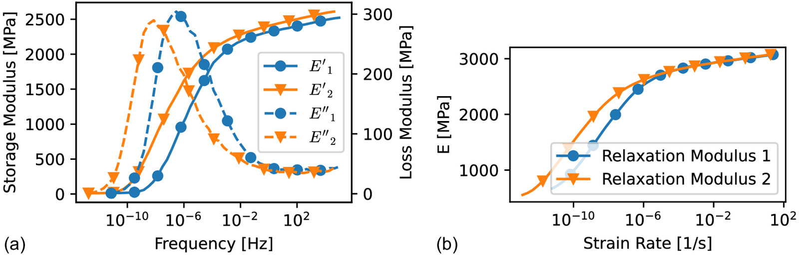
Two single cantilever DMA measurements were performed in the temperature range of 0°C to 120°C for 10 logarithmic distributed frequencies in the range of 1–25 Hz and with an amplitude of . The specimens with dimensions were separated from a molded plate. A Cole-Cole plot was used to identify the range of evaluable measurement data (see Fig. 3). Therefore, the measured values in the temperature range from 0°C to 100°C were used to create a master curve at 25°C for the storage modulus as a function of the angular frequency using the time-temperature superposition principle [see Fig. 4(a)]. As shown in Zeltmann et al. (2016), DMA could be used to investigate the strain rate dependence of Young’s modulus. For this, a generalized Maxwell model was fitted to the master curve using the python package scipy version 1.10.0. The fit required 12 resp. 14 Prony terms. The normalized standard deviation of the parameters found did not exceed 9%. Using the generalized Maxwell model, the time-dependent relaxation modulus was calculated according to Eq. (9) as follows:with , , being the instantaneous Young’s Modulus and the parameters of the Prony term . For the instantaneous Young’s Modulus, a value of was chosen. This value corresponded to Young’s Modulus out of the technical datasheet (Magner and Kautz 2013).
(9)
For a constant strain rate at the beginning at , the time-dependent stresses are given as (Zeltmann et al. 2017)
(10)
For a fixed strain (here, 0.005), stresses were calculated using Eq. (10) for a range of strain rates; thus, the secant modulus for the fixed strain was calculated at different strain rates. The secant modulus over strain rate is shown in Fig. 4(b). Since only a limited frequency range can be covered by the master curve, only a section of the time domain can be represented. An orientation for the limits of the time domain can be derived from the minimum (0.2 ms) and maximum () relaxation times calculated for the fit of the generalized Maxwell model. The results of the DMA show that the selected strain rate of was in a range where the stiffness of the material showed little dependence on the strain rate, and the effects of the viscoelastic properties of the epoxy were relatively small. Therefore, it was assumed that the material behavior can be approximately described using elastoplastic models. Accordingly, the material behavior was assumed to be elastoplastic in the following investigations unless otherwise indicated.
Tensile Test
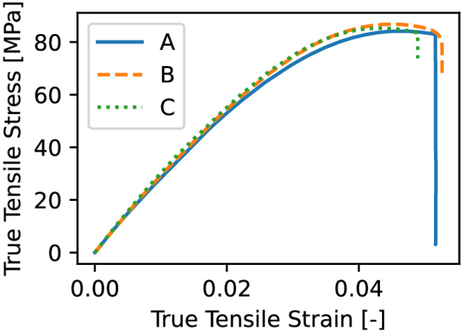
Uniaxial tensile tests were carried out to investigate the parameters of the epoxy resin until the specimen failed. The specimen shape is shown in Fig. 1(b). The longitudinal and transverse strain was measured using a video extensometer. Before investigating the mechanical properties in detail, the influence of the curing cycle was determined. The three different curing cycles were checked, each with 20 specimens. Representative curves for the comparison of the different curing cycles are shown in Fig. 5. No significant property changes resulted from the different curing cycles. Both curing cycles with higher curing temperature showed more scattering of the measured data than did the short curing cycle. This can be attributed to thermally induced residual stresses that lead to small deformations in the specimens. Following this, the shortest curing cycle (cycle C; see section “Material and General Conditions”) was used for every additional test.
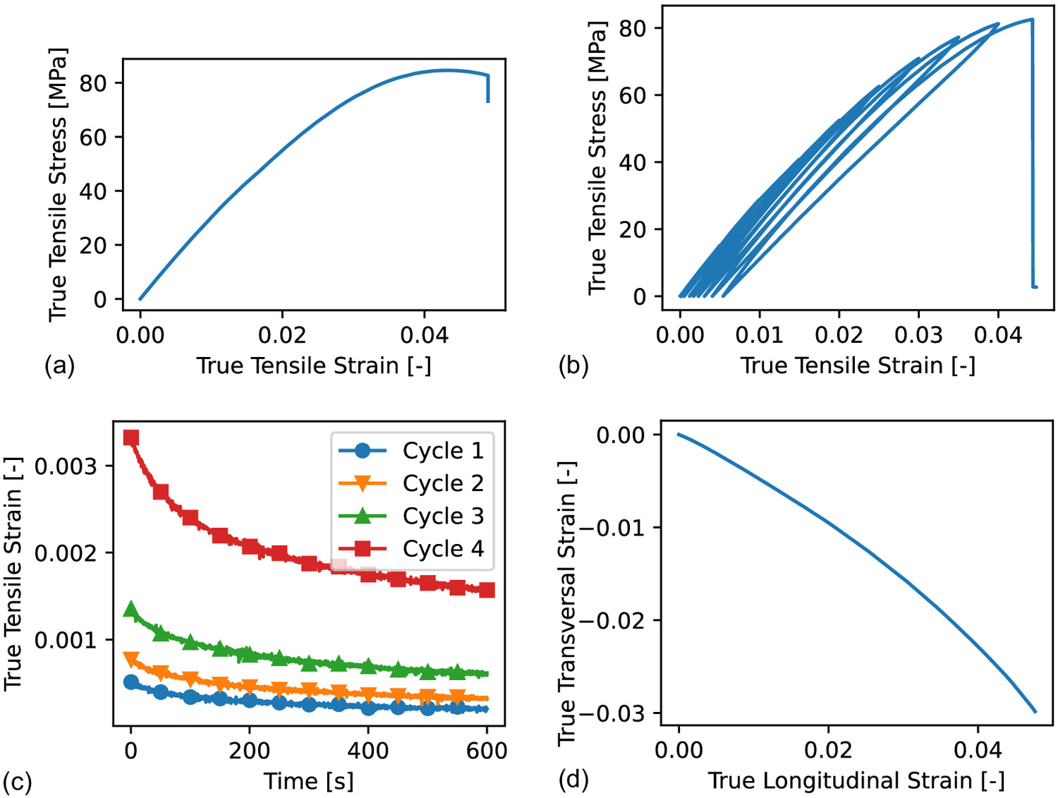
The results of the uniaxial tensile test are shown in Fig. 6(a). The epoxy showed a linear-viscoelastic increase in stress followed by a nonlinear part. Young’s modulus of was observed. Tensile strength of and tensile strain at a break of were measured. To determine the onset of yielding, force-controlled quasistatic loading-unloading tests were performed [see Fig. 6(b)]. The tests showed that the nonlinear stress-strain relation consisted of two components: a viscoelastic part observed from the loading-unloading hysteresis and a plastic part observed from irreversible remaining strains. The irreversible strain remained even for small stresses. To check for strain recovery at zero force, for one specimen, force-controlled holding times of 600 s (approximately twice the test time of the regular tensile test) were held after each unloading cycle; see Fig. 6(c). The results show that irreversible strains remained even at small forces, and no significant recovery of the strains was expected beyond the holding time. Therefore, the yield stress was determined using the linear elastic limit at which 0.1% plastic strain remained after unloading. This procedure was in general agreement with other investigations (Fiedler et al. 2001b; Morelle et al. 2017). A yield stress under tensile load of was determined. In Fig. 6(d), the measured relationship between transverse and longitudinal strain under a tensile load is shown. An overall value of for the elastic Poisson’s ratio in the range of was measured. The range for the evaluation of the elastic Poisson’s ratio was defined such that the measurement inaccuracy of the extensometer was . After onset of yielding, an increase in Poisson’s ratio to values of could be observed. A summary of the measured properties out of the tensile tests is given in Table 1.
| Parameter | Value |
|---|---|
| (MPa) | |
| 0.5 | |
| (MPa) | |
| (MPa) | |
| (MPa) | |
Compression Test
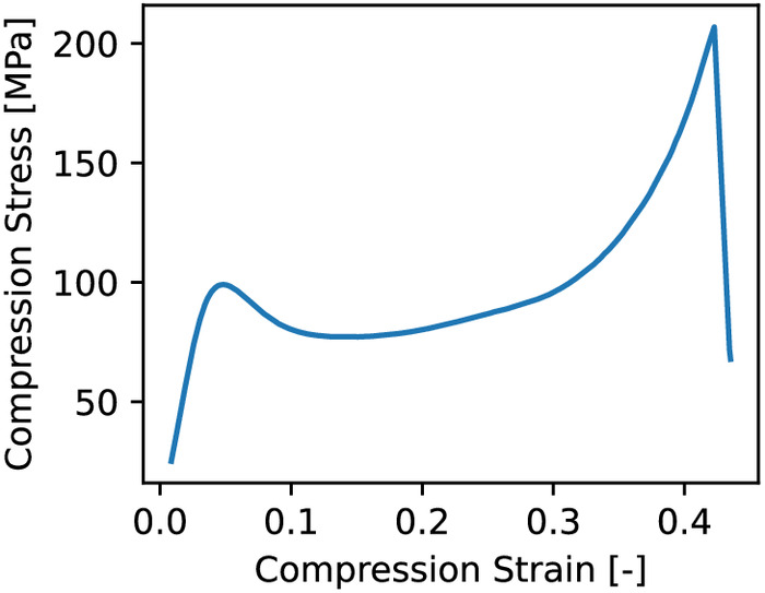
For the compression test, a PTFE foil was used to minimize the friction between the sample [see Fig. 1(d)] and the pressure plates. The results of the compression tests are shown in Fig. 7. In agreement with the tensile tests, at the beginning, the stress increased in a linear-elastic manner before reaching a peak value. The stress-peak was followed by a softening part, leading to a plateau at which the stress stayed nearly constant while the strain increased. After this plateau, the stress increased after fracture of the specimen. From the linear part, Young’s modulus of was observed. The yield stress was observed at . A video extensometer showed that the softening of the material was caused by the development of one macroscopic shear-band after the stress reached the first peak value. Whether this macroscopic shear band described the actual material behavior under compression or was caused by the specimen geometry and the friction between specimen and compression plate must be discussed. The latter represents a general problem in the realization of compression tests. After a strain at a break of , a similar fracture pattern as that obtained by Fiedler et al. (2001b)—with cracks in the loading direction—was detected. As discussed in Roetsch and Horst (2022), material separation under uniaxial compressive stress was caused by shear stresses with simultaneous compressive pressure. The experimental compression strengths determined here represented the stress at which cracking was observed visually and acoustically. The compressive strength reached . Here, it is important to distinguish between true and engineering stresses. Despite the fact that the shear band formation could be recorded by the video extensometer, a measurement of the transverse strain was not possible; therefore, only the initial sample size could be used for stress calculations. Fig. 7 shows engineering stresses. An estimate of the true fracture stress was approximated by measuring a cracked specimen, leading to . A summary of the measured properties out of the compression tests is given in Table 2.
| Parameter | Value |
|---|---|
| (MPa) | |
| (MPa) | |
| (MPa) | |
| (eng.) (MPa) | |
| (true) (MPa) | |
Torsion Test
Torsion tests with different varying axial tensile and compressive loads were performed. Clamping was realized using two precision vices with roughened clamping surfaces. A total of six different tests were carried out, each with five specimens [see Fig. 1(c)]. The tension/compression torsion tests were done with an axial load of and . Furthermore, torsion tests were carried out in which the axial load was controlled to be zero. The deformation of the specimen was measured using the torsion of the clamping. For the evaluation of the torsion tests, assumptions of a uniform deformation of the specimen over the measuring length were made. The applied torque, twist angle, and axial loads and deformations were measured. The relationship between the shear stresses and the applied torque followed Seyda et al. (2020)
(11)
Assuming a linear dependence of the shear stress on the radius , the shear stress is as follows:
(12)
However, the influence of the axial deformation of the specimen due to torsion (Poynting effect) was not taken into account. Assuming that the outer and inner radius , of the specimens changed by the same difference , the radii of the specimens as a function of the axial deformations led toandwhere = initial wall thickness; and is the Hencky strain in the axial direction. Thus, using Eqs. (13) and (14), Eq. (12) gives the true shear stress. The distortion follows withwhere = twist angle. This approach takes into account the axial deformation of the specimen due to torsion (Poynting effect). A similar approach by Wu et al. (1997) was used, for example, for an analysis of aluminum and steel specimens under torsion (Lu et al. 2021).
(13)
(14)
(15)
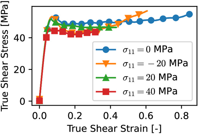
The results of the torsion tests are shown in Fig. 8. For each test, a shear modulus of was measured. Yielding was defined using a linear elastic limit of , leading to a yield stress of for an axial load of zero. No major changes were observed in the yield stresses at different axial loads. The combined compression-torsion tests with an axial load of was not evaluated due to buckling of the specimens. The shear strength at an axial load of zero reached . Given increasing axial tension, a decrease in the shear strength was observed. Moreover, a slightly decrease in shear strength was measured for increased axial compression load. After reaching the shear strength, a softening part and a constant stress plateau with large shear strain was observed. This large plastic deformation under torsion load seemed typical for epoxy (Fiedler et al. 2001b; Littell et al. 2008). With axial load, especially with tension load, a significant reduction in the strain at a break was observed. A summary of the measured properties out of the torsion tests is given in Table 3.
| (MPa) | (MPa) | (MPa) | (MPa) | (MPa) | |
|---|---|---|---|---|---|
| 0 | |||||
| 20 | |||||
| 40 |
Poker Chip Test
Various methods have evolved to generate triaxial tensile stress states in polymers. Lindsey (1966) used the so-called poker chip test to obtain hydrostatic tensile stress conditions in polyurethane rubber. Here, a disc-shaped specimen is glued between two steel cylinders and ripped apart [see Fig. 1(a)]. Asp et al. (1995) and Kim et al. (2013) adopted this test setup for the mechanical characterization of epoxy resin under triaxial tensile loads. A different method was used by Gross et al. (2017). Here, an epoxy resin was cooled from the curing temperature inside a quartz tube. As a result of the cooling, the epoxy resin contracts, which was hindered by its adhesion to the walls of the quartz tube. The results show similar reduced strengths to those observed in the poker chip test (Gross et al. 2017).
Therefore, the poker chip test appears to be an adequate way to investigate the mechanical behavior of the epoxy resin under triaxial tensile loading. The experimental setup of the poker chip test is shown in Fig. 1. The steel cylinders were sandblasted and decreased with acetone. A silicone O-ring was then placed on the lower cylinder and filled with epoxy resin. The upper steel cylinder was then placed on the still liquid epoxy resin and the O-ring. In contrast to Asp et al. (1995), this procedure does not require subsequent bonding of the specimen. The inner diameter (30 mm) and thickness (4 mm) of the O-ring specify the specimen’s geometry. The resin was cured in the same way as the tensile, compression, and torsion specimens.
The axial deformation was measured using the machine cross head (the deformation of the machine was corrected). Lindsey (1966) analyzed in detail the stress and deformation state of the poker chip sample in the elastic regime. The specimen with normalized radius was deformed in the direction by . The radius was normalized by half the specimen thickness such that the aspect ratio of the specimen corresponds to the normalized radius (Lindsey 1966; Asp et al. 1995). The stresses within the specimen are given in simplified form by Lindsey (1966)where , = Young’s modulus and the Poisson’s ratio; , , , = normal and shear stresses in the direction of the polar coordinates , , ; and , = normalized specimen radius and nominal strain. , are zero- and first-order modified Bessel functions. The stress distribution in the center of the sample is shown in Fig. 9.
(16)
(17)
(18)
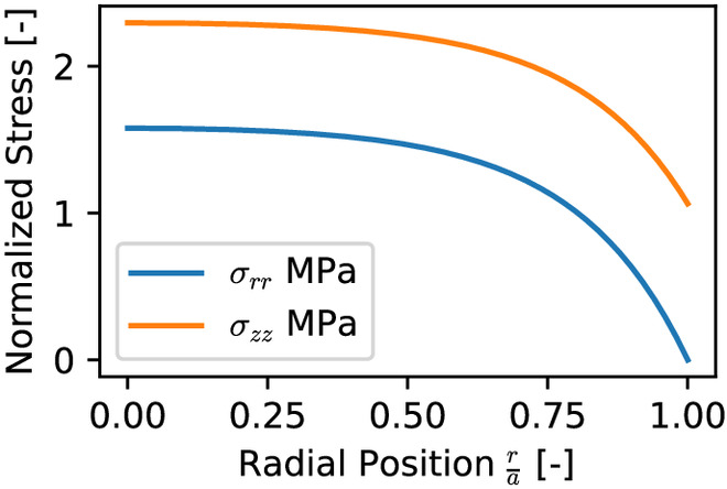
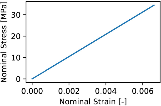
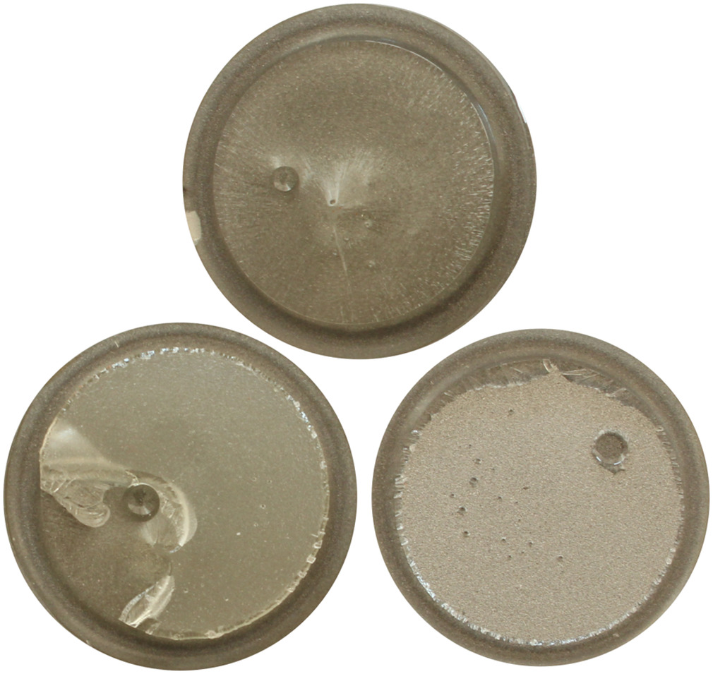
All specimens tested showed linear elastic material behavior to failure (see Fig. 10). A total of 20 specimens were tested, and three different failure modes were observed (see Fig. 12). Half of the samples showed a cohesive fracture in the middle of the sample. The other half showed both complete adhesive fracture (failure of the interface) and a mixture of cohesive and adhesive fractures. Only the samples with cohesive failure were used for further investigation. An apparent Young’s modulus of and an apparent strength of with an elongation at a break of were measured. Eqs. (16)–(18) follow an actual stress distribution in the center of the specimens of , , which corresponds to a stress ratio of approximately . From Eq. (1), a hydrostatic tensile strength of was obtained for this stress distribution. Eq. (8) predicts a value of , which is a good estimate in the case of missing experimental data for . A summary of the results for the poker chip test is given in Table 4.
| Parameter | Value |
|---|---|
| (MPa) | |
| (MPa) | |
| (MPa) | 33.5 |
| (MPa) | 28.13 |
Fracture Behavior
Fig. 11 shows the tensile, compression, and torsion specimens used before and after the tests (only compression specimens after the tests). The tensile and compression tests show fracture surfaces perpendicular and parallel to the loading direction, respectively.
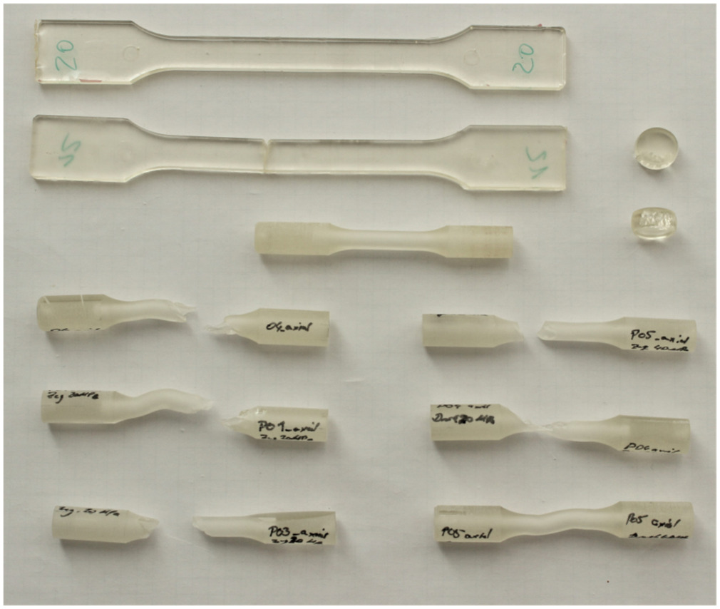
Fig. 12 shows the three failure modes for the poker chip test performed. The single air inclusions in the specimens are a result of the manufacturing process described. However, no correlation was observed between the location of the crack initiation and the presence of air inclusions. Moreover, no correlation with the presence of air inclusions could be established for the measured strengths such that the influence of these imperfections was classified as low. Fig. 12 shows a crack initiation in the center of the specimen near or at the interface. It is noteworthy that for half of the specimens, the crack area propagated to the center (thickness direction) of the specimen instead of progressing at the interface with the steel cylinders. This indicates a very critical stress state within the specimen. Scanning electron microscope (SEM) micrographs of the fracture surface were performed using a Zeiss EVO MA15 microscope (Carl Zeiss AG, Oberkochen, Germany). The SEM pictures of the fracture surface from the poker chip test are shown in Fig. 12 and for the uniaxial tensile tests in Fig. 13. Uniaxial tension typical fracture surfaces, such as those observed by Cantwell et al. (1988), Bandyopadhyay (1990), Fiedler et al. (2001b), and Morelle et al. (2017), can be investigated. Accordingly, a mirror-like surface is present around the crack initiation region due to continuously (slow) crack propagation. As the crack propagation progressed, the crack velocity increased, and secondary cracks developed because of the high local stresses that results in a rougher fracture surface.
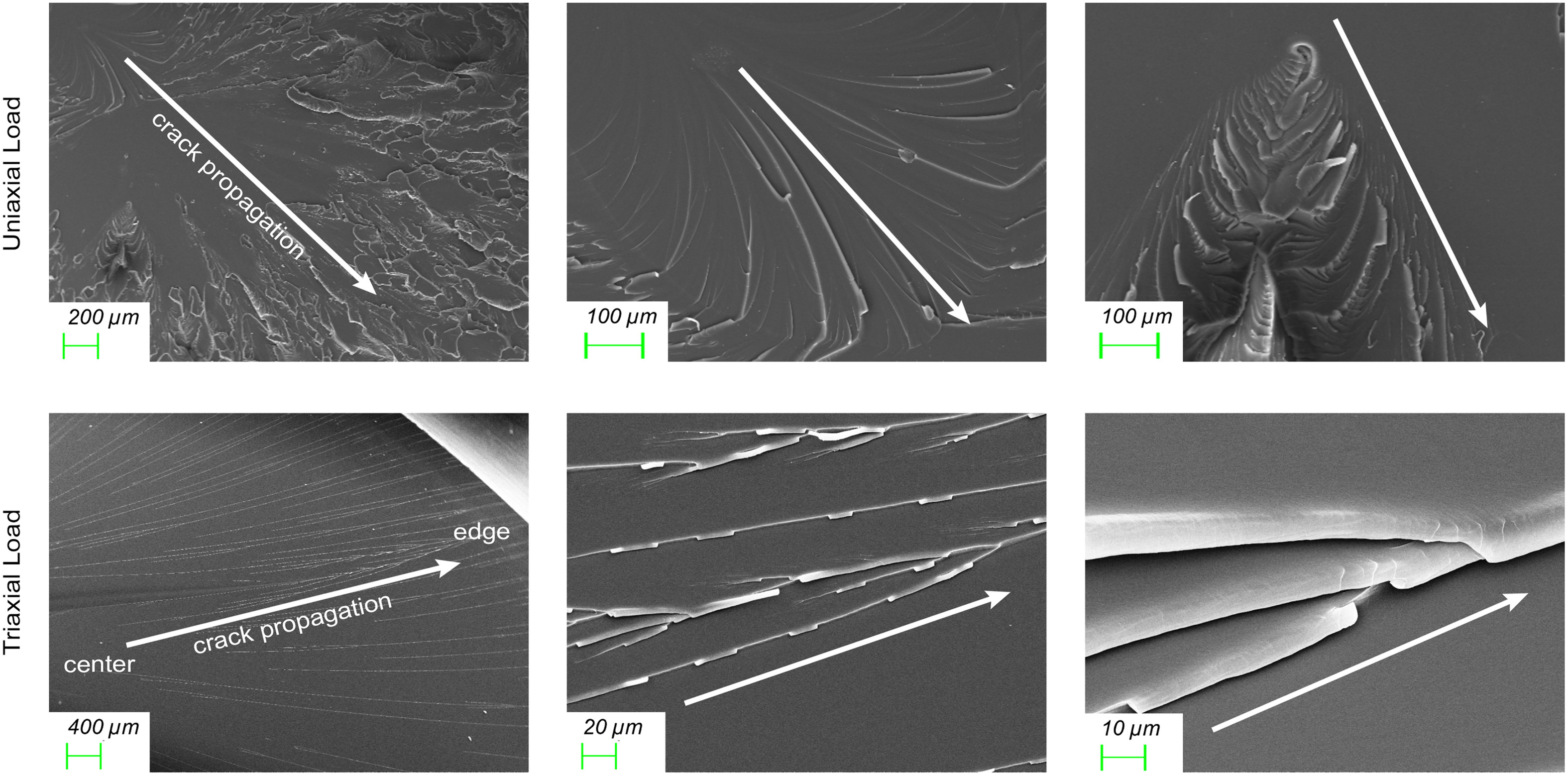
The complete fracture surface of the poker chip specimen is mirror-like and nearly featureless, similar to the fracture surface for uniaxial tension near crack initiation. The smooth fracture surface corresponds to a continuously accelerating single crack (Cantwell et al. 1988; Bandyopadhyay 1990). As crack propagation progressed, radially aligned step-like (river-like) secondary cracks formed that partially coalesced toward the edge of the specimen. This is in general agreement with the observations from Asp et al. (1995) for a Diglycidyl Ether of Bisphenol A (DGEBA) epoxy system with aliphatic curing agents. Since the crack initiation is near the interface, and the crack progresses to the middle of the specimen, the single secondary cracks could be in different planes. The coalesce of those step-like cracks may be the result of the height adjustment of single cracks.
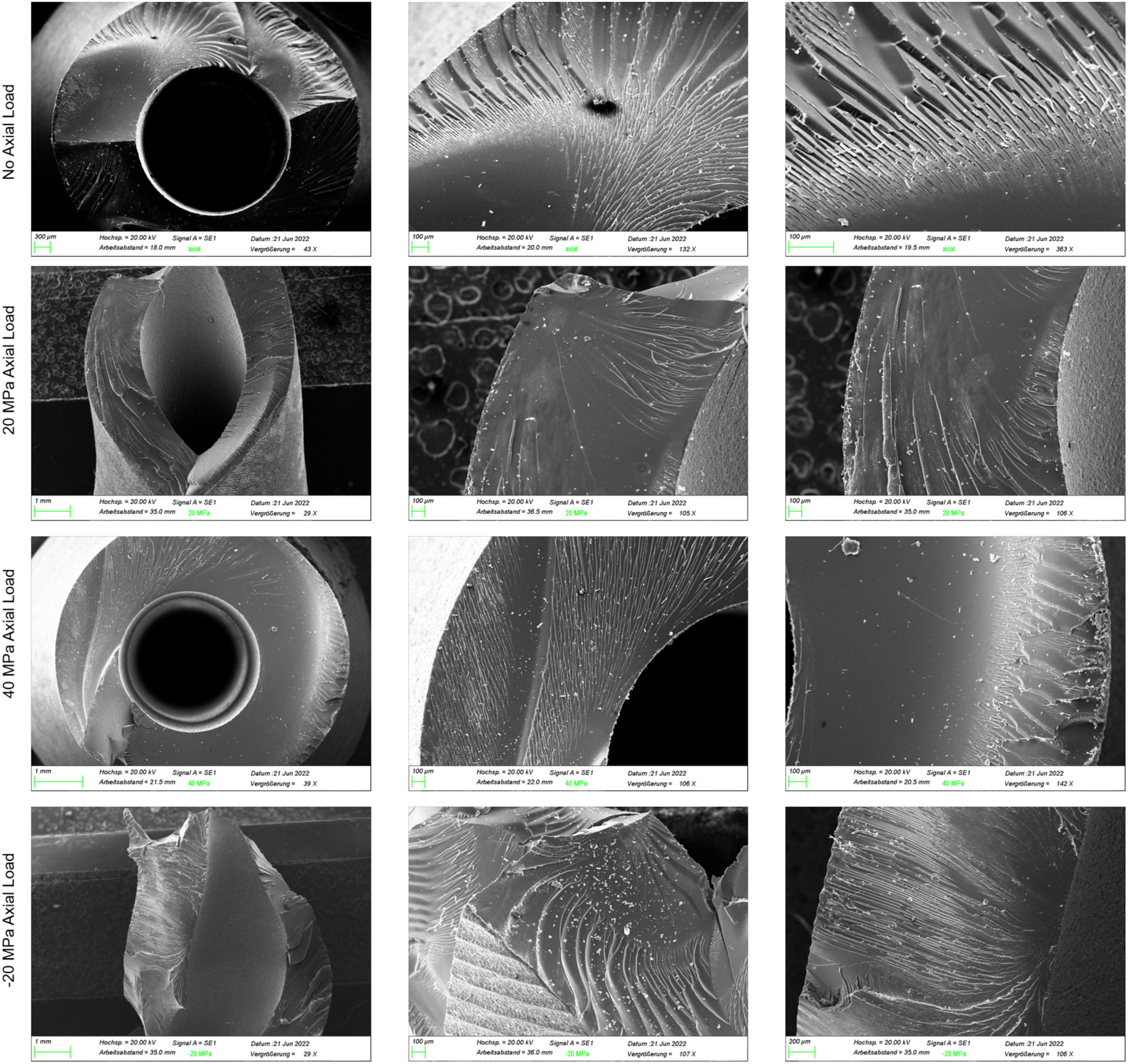
In the torsion test, nearly all torsion specimens failed at a 45° angle to the longitudinal axis of the specimen. This indicates a failure due to the largest principal tensile stress. Some fracture surfaces also showed smaller fracture angles, which indicates an additional contribution of the largest shear stress. The typical fracture surface of the torsion specimens is shown in Fig. 14. All fracture surfaces exhibited three characteristic details that were pronounced to different degrees. These characteristics included a mirror-like event-free surface, a finely textured surface with parallel river-like scratches, and areas with large steps. In Morelle et al. (2017), the smooth fracture surface (mirror-like) was associated with fracture initiation and slow fracture progression. The area with finely distributed scratches (river-like) follows this smooth fracture surface. This surface was also observed in the poker chip tests. With crack propagation, these fine scratches developed into larger steps, which could only be observed in this way in the torsion specimens and agree with observations by Fiedler et al. (2001b) (transition from river-like to step-like). Fiedler et al. (2001b) considered the cause for the structure of this fracture surface to be a superposition of normal and shear stress driven cracks, where the shear stresses lead to plastic deformation.
Comparison to Failure Criteria
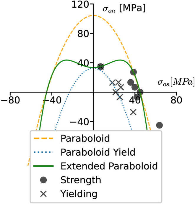
Fig. 15 shows the comparison of the determined yield stresses and strengths with the predictions of the paraboloid criterion and the extended paraboloid criterion. Since the extended paraboloid criterion is designed as a strength criterion, the comparison with the yield stresses is restricted to the predictions of the classical paraboloid criterion of Stassi-D’Alia (1967). The scaling of the criteria was done using the uniaxial tensile strength and the shear strength. The triaxial tensile strength determined in the poker chip test was also included in the yield criterion.
A physical interpretation of the paraboloid yield criterion when applied to epoxy resin could be the rotation of chain segments caused by deviatoric parts of the stress tensor and the initiation of nanovoids as a result of the volumetric part of the stress tensor, which could explain the pressure-dependent yield behavior. In addition, the final failure, especially under tensile load, could be explained by the formation of voids, which can be described by the volumetric dilatation energy criterion (Asp et al. 1996). The extended paraboloid criterion thus represents a combination of these mechanisms.
From the perspective of material modeling, the yield criterion transforms into a strength criterion through hardening processes. Assuming that no yielding occurs under hydrostatic tension (Roetsch and Horst 2022), the yield and strength criteria must match in this point. The paraboloid criterion shows good agreement with the measured yield stresses and tended to be a more conservative estimate.
A comparison of the two criteria with the measured strengths reveals the significant differences in the range of triaxial tension. While the criteria in the range of uniaxial tension, torsion, and uniaxial compression make almost identical predictions, the classical paraboloid criterion overestimates the measured triaxial tensile strength by approximately three times. The extended paraboloid criterion can provide exact agreement with the results from the poker chip test. For the uniaxial compression test, the estimated value of is included (see section “Compression Test”).
Model Implementation
In the following, how the extended paraboloid criterion can be applied in the context of damage mechanics is shown.
Constitutive Equations
For the elastoplastic material behavior of the epoxy resin, the material model by Melro et al. (2013), Melro (2011), and van der Meer and van der Meer (2016) was used. The yield criterion corresponds to the paraboloid criterion of Stassi-D’Alia (1967) and has been reformulated into a dependence on the tensile yield stress and the yield stress under shear
(19)
The plastic strain increment is obtained via a nonassociated yield rule towhere
(20)
(21)
Isotropic hardening is defined by the dependence of the yield stresses on the equivalent plastic strain via two section-wise defined functionsandwhere the increment of the equivalent plastic strain is calculated as follows:
(22)
(23)
(24)
In the original model, the plastic multiplier is numerically calculated using a Newton-Raphson scheme (Melro et al. 2013). This algorithm shows high sensitivity on the initial guess value and, especially under compression load, no solution is found. To circumvent this problem, Brent’s method was implemented as an alternative solution method for the plastic multiplier. The implementation was accomplished according to Press (2007).
Damage Model
In continuum damage mechanics (CDM), the damage of a material is described using a damage parameter that degrades its stiffness (Simo and Ju 1987)
(25)
The implementation of Eq. (1) in the context of CDM follows the approach of Melro et al. (2013), where a damage function is introduced
(26)
Here, = local internal variable; and = extended paraboloid criterion introduced in Eq. (1) formulated using effective stresses . The degradation of the stiffness leads to a softening of the material. Implementing CDM models in FE analyses leads to a dependence of the solution on the size of the finite elements. To regularize the localization effect, an implicit gradient model introduced by Peerlings et al. (1996) is usedwhere = nonlocal counterpart to the internal variable . Additionally, the following Neumann boundary conditions are used
(27)
(28)
Damage onset is defined if ; therefore, in the damage regime, the condition must hold. The evolution of the damage variable is defined using the following damage evolution law
(29)
The history variable is related to the nonlocal variable via Kuhn-Tucker relations (Peerlings et al. 1996)
(30)
The irreversibility of the damage process and the definition for follows from the Kuhn-Tucker relations (Simo and Ju 1987)
(31)
To ensure that damage initiation remains a local event, this definition for is extended (Seupel et al. 2018)
(32)
Therefore, even if the value of the nonlocal variable exceeds one, the history variable is initially updated only if the local variable also exceeds one. This model was implemented as a user-subroutine UMAT in Abaqus version 2021, the commercial finite element analysis (FEM) software. The implementation of the implicit gradient model within UMAT is done using the heat-damage analogy introduced by Seupel et al. (2018). For this, the nondiagonal coupling terms of the displacement-phase field stiffness matrix were set to zero. This leads to a slower convergence rate but makes the implementation easier since the derivative is not needed (Navidtehrani et al. 2021, 2022). For the implementation using a UMAT subroutine, the following derivatives need to be defined:where = consistent tangent operator out of the plasticity model. The principal deduction for is shown in van der Meer and van der Meer (2016).
(33)
(34)
(35)
Model Predictions
The input parameters used for the material model are listed in Table 5. The input variables required for the hardening law were taken directly from the measured curves of the tension and torsion tests and are provided in Table 6.
| Parameter | Value |
|---|---|
| (MPa) | 3,100 |
| 0.41 | |
| 0.5 | |
| (MPa) | 82 |
| (MPa) | 55 |
| (MPa) | 33.5 |
| (MPa) | (MPa) | |
|---|---|---|
| 0.0 | 38.0070437 | 32.1290964 |
| 0.00030612 | 41.9960619 | 34.0484586 |
| 0.00061224 | 44.6082353 | 35.437616 |
| 0.00091837 | 47.7242899 | 36.9586479 |
| 0.00122449 | 51.2279779 | 38.6100483 |
| 0.00153061 | 54.3200536 | 39.9791754 |
| 0.00183673 | 56.9906606 | 41.1674816 |
| 0.00214286 | 59.3920513 | 42.2420135 |
| 0.00244898 | 61.5711432 | 43.2038994 |
| 0.0027551 | 63.5348803 | 44.0752071 |
| 0.00306122 | 65.3031808 | 44.8623296 |
| 0.00336735 | 66.9203979 | 45.5406266 |
| 0.00367347 | 68.3937671 | 46.1627481 |
| 0.00397959 | 69.7408152 | 46.735293 |
| 0.00428571 | 70.9682955 | 47.2530337 |
| 0.00459184 | 72.1032641 | 47.7363252 |
| 0.00489796 | 73.1530548 | 48.1883068 |
| 0.00520408 | 74.1146521 | 48.599188 |
| 0.0055102 | 75.0176844 | 48.9830374 |
| 0.00581633 | 75.8560494 | 49.3249319 |
| 0.00612245 | 76.6185283 | 49.6403296 |
| 0.00642857 | 77.3352697 | 49.9372043 |
| 0.00673469 | 77.985558 | 50.2082491 |
| 0.00704082 | 78.6051674 | 50.4611423 |
| 0.00734694 | 79.1667004 | 50.693837 |
| 0.00765306 | 79.6952732 | 50.9130853 |
| 0.00795918 | 80.1789696 | 51.1159989 |
| 0.00826531 | 80.6354991 | 51.3073259 |
| 0.00857143 | 81.0498932 | 51.4777375 |
| 0.00887755 | 81.4400795 | 51.6327687 |
| 0.00918367 | 81.7842953 | 51.773374 |
| 0.0094898 | 82.1187961 | 51.9115142 |
| 0.00979592 | 82.4189995 | 52.0358292 |
| 0.01010204 | 82.694825 | 52.142293 |
| 0.01040816 | 82.9470357 | 52.2412334 |
| 0.01071429 | 83.1742307 | 52.3293854 |
| 0.01102041 | 83.3913577 | 52.4133323 |
| 0.01132653 | 83.5733826 | 52.4838795 |
| 0.01163265 | 83.7451058 | 52.5490203 |
| 0.01193878 | 83.8941434 | 52.6062297 |
| 0.0122449 | 84.0265361 | 52.6544649 |
| 0.01255102 | 84.1517346 | 52.7004245 |
| 0.01285714 | 84.2551756 | 52.7371636 |
| 0.01316327 | 84.3426051 | 52.7687529 |
| 0.01346939 | 84.4236283 | 52.795629 |
| 0.01377551 | 84.4792433 | 52.8127981 |
| 0.01408163 | 84.5312817 | 52.828655 |
| 0.01438776 | 84.5768738 | 52.8393103 |
| 0.01469388 | 84.5983804 | 52.8424379 |
| 0.015 | 84.6135588 | 52.8416312 |
| 0.4 | — | 52.8416312 |
| 0.48769639 | — | 55.0 |
The comparison of the model predictions for a one element test case with the experimentally determined curves is shown in Figs. 16 and 17. Since the model was fitted via tensile and torsional curves, the material model provides very good agreement here. Given compression, the yield point is predicted well; however, the simulated curve deviates significantly from the experimental curve, for various possible reasons. On the one hand, technical stresses and strains are shown here for the compression case. Furthermore, a softening after an initial stress peak is observed in the measurements for both torsion and compression. Taking this softening into account via the hardening parameters under torsion leads to very good agreement for the values under compression. However, for finite element (FE) models with several elements, this softening needs to be regulated similarly to the case of damage to ensure a mesh-independent solution. This was not considered within the scope of this study. A possible approach to this was presented by, for example, Nguyen et al. (2016). However, the model shows good agreement with the measured fracture strains. Furthermore, both the very ductile material behavior under torsion and the ideally brittle material behavior under hydrostatic tension can in principle be represented by the model.
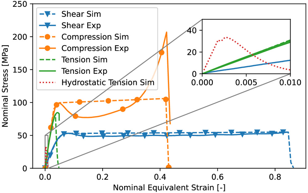
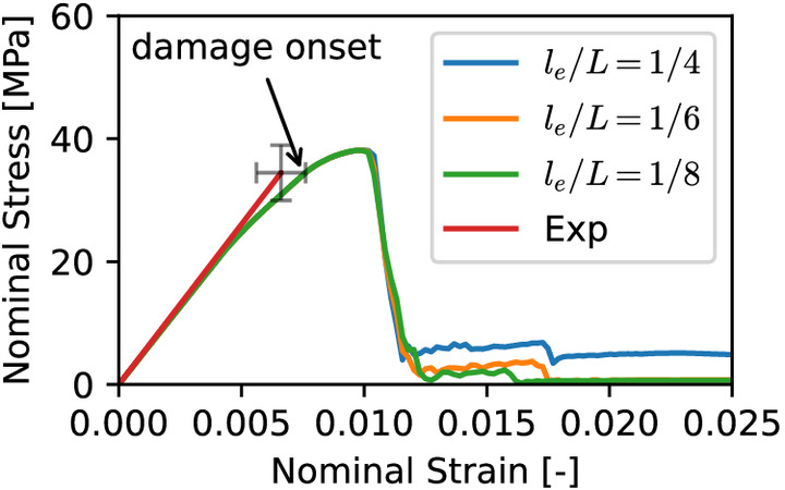
Fig. 17 shows the applicability of the extended paraboloid criterion to accounting for triaxial tensile stresses. The poker chip test is simulated using a rotational-symmetric FE model. Three different characteristic element sizes were used. The parameter was set to 0.5 mm. The strain at damage onset corresponds well with the strain at the breakout of the experiment. The model leads to a slight overprediction of the maximum stress and the strain at a break. The latter could be due to the damage propagating too slowly. No relevant plastic deformation was observed in the simulation of the poker chip test.
Conclusion
In the present work, the mechanical behavior of a typical epoxy resin for the production of fiber-reinforced composites was investigated under uni, bi, and triaxial quasi-static stress conditions. Furthermore, the viscoelastic material behavior was investigated using DMA to ensure that the viscoelastic part is sufficiently small at the tested strain rates, and an elastic-plastic model is suitable for describing the material behavior. The results show that
•
Massive differences were found in material behavior as a function of load type. These results confirm previous studies on the mechanical behavior of epoxy resin (Fiedler et al. 2001a; Morelle et al. 2017; Gerlach et al. 2008; Littell et al. 2008; Asp et al. 1995). Ductile material behavior is particularly evident under compressive and shear loading. This contrast with a mainly brittle material behavior under uniaxial tension and an ideally brittle behavior under triaxial tension. Under torsional loading, both overlaid tensile stress and overlaid compressive stress decrease the strain and the stress at a break. However, only one series of measurements under overlaid compressive stress could be evaluated. Further torsion measurements under compression, in which, for example, buckling of the specimen is prevented, could extend the knowledge of the mechanical behavior of epoxy resin under this loading condition.
•
The poker chip test used by Asp et al. (1995) was successfully applied. A simplified method for sample production using silicone O-rings was presented. Significantly reduced strength compared to the uniaxial tensile strength was demonstrated in a triaxial stress state. This confirms, in particular, the results of Asp et al. (1995).
•
The measured strengths were compared with the paraboloid and extended paraboloid strength criteria. Both were formulated using tensile and shear strength and provide nearly identical predictions in the range of the torsional tests performed. However, since the extended paraboloid criterion also takes into account the hydrostatic tensile strength, a significantly better representation of the material behavior is achieved here than with the paraboloid criterion. In the case of missing experimental data for , the prediction from Eq. (8) is a good alternative.
•
Furthermore, a simple implementation of the extended paraboloid criterion in the context of damage mechanics is possible via the heat-damage analogy introduced by Seupel et al. (2018), and the wide mechanical behavior of epoxy resin can be described approximately together using elastoplastic material behavior.
Data Availability Statement
Some or all data, models, or code that support the findings of this study are available from the corresponding author upon reasonable request.
Acknowledgments
The research was financed by the Saxon State Ministry for Science and the Arts within Project Nos. 2057400300 and 360049 and by the European Social Fund. Financial support is gratefully acknowledged.
References
Asp, L., L. Berglund, and R. Talreja. 1996. “A criterion for crack initiation in glassy polymers subjected to a composite-like stress state.” Compos. Sci. Technol. 56 (11): 1291–1301. https://doi.org/10.1016/S0266-3538(96)00090-5.
Asp, L. E., L. A. Berglund, and P. Gudmundson. 1995. “Effects of a composite-like stress state on the fracture of epoxies.” Compos. Sci. Technol. 53 (1): 27–37. https://doi.org/10.1016/0266-3538(94)00075-1.
Bandyopadhyay, S. 1990. “Review of the microscopic and macroscopic aspects of fracture of unmodified and modified epoxy resins.” Mater. Sci. Eng., A 125 (2): 157–184. https://doi.org/10.1016/0921-5093(90)90167-2.
Cantwell, W. J., A. C. Roulin-Moloney, and T. Kaiser. 1988. “Fractography of unfilled and particulate-filled epoxy resins.” J. Mater. Sci. 23 (5): 1615–1631. https://doi.org/10.1007/BF01115700.
Chevalier, J., X. Morelle, P. Camanho, F. Lani, and T. Pardoen. 2019. “On a unique fracture micromechanism for highly cross-linked epoxy resins.” J. Mech. Phys. Solids 122 (Feb): 502–519. https://doi.org/10.1016/j.jmps.2018.09.028.
Fiedler, B., M. Hojo, S. Ochiai, K. Schulte, and M. Ando. 2001a. “Failure behavior of an epoxy matrix under different kinds of static loading.” Compos. Sci. Technol. 61 (11): 1615–1624. https://doi.org/10.1016/S0266-3538(01)00057-4.
Fiedler, B., M. Hojo, S. Ochiai, K. Schulte, and M. Ochi. 2001b. “Finite-element modeling of initial matrix failure in CFRP under static transverse tensile load.” Compos. Sci. Technol. 61 (1): 95–105. https://doi.org/10.1016/S0266-3538(00)00198-6.
Gerlach, R., C. R. Siviour, N. Petrinic, and J. Wiegand. 2008. “Experimental characterisation and constitutive modelling of RTM-6 resin under impact loading.” Polymer 49 (11): 2728–2737. https://doi.org/10.1016/j.polymer.2008.04.018.
Gross, T. S., H. Jafari, J. Kusch, I. Tsukrov, B. Drach, H. Bayraktar, and J. Goering. 2017. “Measuring failure stress of RTM6 Epoxy Resin under purely hydrostatic tensile stress using constrained tube method.” Exp. Tech. 41 (1): 45–50. https://doi.org/10.1007/s40799-016-0153-2.
Kim, J. W., G. A. Medvedev, and J. M. Caruthers. 2013. “Observation of yield in triaxial deformation of glassy polymers.” Polymer 54 (11): 2821–2833. https://doi.org/10.1016/j.polymer.2013.03.042.
Lindsey, G. H. 1966. Hydrostatic tensile fracture of a polyurethane elastomer. Fort Belvoir, VA: Defense Technical Information Center.
Littell, J. D., C. R. Ruggeri, R. K. Goldberg, G. D. Roberts, W. A. Arnold, and W. K. Binienda. 2008. “Measurement of epoxy resin tension, compression, and shear stress–strain curves over a wide range of strain rates using small test specimens.” J. Aerosp. Eng. 21 (3): 162–173. https://doi.org/10.1061/(ASCE)0893-1321(2008)21:3(162).
Lu, W.-Y., H. Jin, J. Foulk, J. Ostien, S. Kramer, and A. Jones. 2021. “Solid cylinder torsion for large shear deformation and failure of engineering materials.” Exp. Mech. 61 (2): 307–320. https://doi.org/10.1007/s11340-020-00620-6.
Magner, J., and D. Kautz. 2013. Prüfung des Epoxidharz-Systems R&G Epoxydharz L und R&G Härter GL 1. Flörsheim-Wicker, Germany: Kiwa Polymer Institut GmbH.
Melro, A., P. Camanho, F. Andrade Pires, and S. Pinho. 2013. “Micromechanical analysis of polymer composites reinforced by unidirectional fibres: Part I–Constitutive modeling.” Int. J. Solids Struct. 50 (11–12): 1897–1905. https://doi.org/10.1016/j.ijsolstr.2013.02.009.
Melro, A. R. 2011. “Analytical and numerical modelling of damage and fracture of advanced composites.” Ph.D. thesis, Faculty of Engineering, Univ. of Porto.
Morelle, X. P., J. Chevalier, C. Bailly, T. Pardoen, and F. Lani. 2017. “Mechanical characterization and modeling of the deformation and failure of the highly crosslinked RTM6 epoxy resin.” Mech. Time-Depend Mater. 21 (3): 419–454. https://doi.org/10.1007/s11043-016-9336-6.
Navidtehrani, Y., C. Betegón, and E. Martínez-Pañeda. 2021. “A unified abaqus implementation of the phase field fracture method using only a user material subroutine.” Materials 14 (8): 1913. https://doi.org/10.3390/ma14081913.
Navidtehrani, Y., C. Betegón, and E. Martínez-Pañeda. 2022. “A general framework for decomposing the phase field fracture driving force, particularised to a Drucker–Prager failure surface.” Theor. Appl. Fract. Mech. 121 (Sep): 103555. https://doi.org/10.1016/j.tafmec.2022.103555.
Neogi, A., N. Mitra, and R. Talreja. 2018. “Cavitation in epoxies under composite-like stress states.” Composites, Part A 106 (Apr): 52–58. https://doi.org/10.1016/j.compositesa.2017.12.003.
Nguyen, V.-D., F. Lani, T. Pardoen, X. Morelle, and L. Noels. 2016. “A large strain hyperelastic viscoelastic-viscoplastic-damage constitutive model based on a multi-mechanism non-local damage continuum for amorphous glassy polymers.” Int. J. Solids Struct. 96 (Jun): 192–216. https://doi.org/10.1016/j.ijsolstr.2016.06.008.
Peerlings, R. H. J., R. De Borst, W. A. M. Brekelmans, and J. H. P. De Vree. 1996. “Gradient enhanced damage for quasi-brittle materials.” Int. J. Numer. Methods Eng. 39 (19): 3391–3403. https://doi.org/10.1002/(SICI)1097-0207(19961015)39:19%3C3391::AID-NME7%3E3.0.CO;2-D.
Poulain, X. M. N. 2010. “On the thermomechanical behavior of epoxy polymers: Experiments and modeling.” Ph.D. thesis, Dept. of Aerospace Engineering, Texas A&M Univ.
Press, W. H. 2007. “Numerical recipes in Fortran 77: The art of scientific computing.” In Number 1 in Fortran numerical recipes. 2nd ed. Cambridge, UK: Cambridge University Press.
Roetsch, K., and T. Horst. 2022. “A novel approach to consider triaxial tensile stresses within the framework of a failure criterion.” Z. Angew. Math. Mech. 102 (7): e202100232. https://doi.org/10.1002/zamm.202100232.
Seupel, A., G. Hütter, and M. Kuna. 2018. “An efficient FE-implementation of implicit gradient-enhanced damage models to simulate ductile failure.” Eng. Fract. Mech. 199 (Apr): 41–60. https://doi.org/10.1016/j.engfracmech.2018.01.022.
Seyda, J., Ł. Pejkowski, and D. Skibicki. 2020. “The shear stress determination in tubular specimens under torsion in the elastic-plastic strain range from the perspective of fatigue analysis.” Materials 13 (23): 5583. https://doi.org/10.3390/ma13235583.
Simo, J. C., and J. W. Ju. 1987. “Strain- and stress-based continuum damage models–I. Formulation.” Int. J. Solids Struct. 23 (7): 821–840. https://doi.org/10.1016/0020-7683(87)90083-7.
Singh, G., D. Kumar, and P. M. Mohite. 2017. “Damage modelling of epoxy material under uniaxial tension based on micromechanics and experimental analysis.” Arch. Appl. Mech. 87 (4): 721–736. https://doi.org/10.1007/s00419-016-1219-4.
Stassi-D’Alia, F. 1967. “Flow and fracture of materials according to a new limiting condition of yelding.” Meccanica 2 (3): 178–195. https://doi.org/10.1007/BF02128173.
Sundararaghavan, V., and A. Kumar. 2013. “Molecular dynamics simulations of compressive yielding in cross-linked epoxies in the context of Argon theory.” Int. J. Plast. 47 (Apr): 111–125. https://doi.org/10.1016/j.ijplas.2013.01.004.
van der Meer, F., and F. P. van der Meer. 2016. “Micromechanical validation of a mesomodel for plasticity in composites.” Eur. J. Mech. A Solids 60 (Jun): 58–69. https://doi.org/10.1016/j.euromechsol.2016.06.008.
Wan, L., Y. Ismail, Y. Sheng, J. Ye, and D. Yang. 2023. “A review on micromechanical modelling of progressive failure in unidirectional fibre-reinforced composites.” Composites, Part C 10 (Mar): 100348. https://doi.org/10.1016/j.jcomc.2023.100348.
Werner, B., and I. Daniel. 2014. “Characterization and modeling of polymeric matrix under multi-axial static and dynamic loading.” Compos. Sci. Technol. 102 (Sep): 113–119. https://doi.org/10.1016/j.compscitech.2014.07.025.
Wu, H.-C., Z. Xu, and P. T. Wang. 1997. “Determination of shear stress-strain curve from torsion tests for loading-unloading and cyclic loading.” J. Eng. Mater. Technol. 119 (1): 113–115. https://doi.org/10.1115/1.2805963.
Wu, Z., S. Ahzi, E. M. Arruda, and A. Makradi. 2005. “Modeling the large inelastic deformation response of non-filled and silica filled SL5170 cured resin.” J. Mater. Sci. 40 (17): 4605–4612. https://doi.org/10.1007/s10853-005-0903-5.
Zeltmann, S. E., B. B. Kumar, M. Doddamani, and N. Gupta. 2016. “Prediction of strain rate sensitivity of high density polyethylene using integral transform of dynamic mechanical analysis data.” Polymer 101 (Jun): 1–6. https://doi.org/10.1016/j.polymer.2016.08.053.
Zeltmann, S. E., K. A. Prakash, M. Doddamani, and N. Gupta. 2017. “Prediction of modulus at various strain rates from dynamic mechanical analysis data for polymer matrix composites.” Composites, Part B 120 (Sep): 27–34. https://doi.org/10.1016/j.compositesb.2017.03.062.
Information & Authors
Information
Published In

Journal of Engineering Mechanics
Volume 151 • Issue 1 • January 2025
Copyright
This work is made available under the terms of the Creative Commons Attribution 4.0 International license, https://creativecommons.org/licenses/by/4.0/.
History
Received: Mar 22, 2024
Accepted: Jul 31, 2024
Published online: Oct 18, 2024
Published in print: Jan 1, 2025
Discussion open until: Mar 18, 2025
Authors
Metrics & Citations
Metrics
Citations
Download citation
If you have the appropriate software installed, you can download article citation data to the citation manager of your choice. Simply select your manager software from the list below and click Download.