Determination of Fixture-Use Probability for Peak Water Demand Design Using High-Level Water End-Use Statistics and Stochastic Simulation
Publication: Journal of Water Resources Planning and Management
Volume 149, Issue 11
Abstract
Some recent studies have used actual water end-use data to inform the peak demand design of plumbing systems in residential buildings, addressing the problem of overestimation in many long-standing plumbing codes and standards. Vast amounts of fixture-specific data from each household are required to determine the frequency each fixture is used during peak water consumption periods (fixture-use probability). However, obtaining such data can be difficult, and the processing is costly and time-consuming. The current study presents a new approach for determining the fixture-use probability for peak water demand design of premise plumbing systems. A stochastic water demand model is developed using only the high-level statistical information from water end-use studies presented in the public domain, offsetting the need for the original water end-use data sets. The stochastic model is then used to form easy-to-use formulas for determining the probability of use for various fixture groups, which consider both the number of apartments and building occupancy. The approach is validated by comparing the estimated peak demand values with the corresponding values determined from actual water consumption observations in three Australian residential apartment buildings and one mixed-use building. The new approach enables a much more accurate estimation of the peak demand compared with the conventional approach suggested in the current Australian plumbing standard. The proposed approach can be used by researchers and practitioners in other countries to determine their region-specific fixture-use probability values for more accurate peak demand estimation, contributing to improved premise plumbing system design.
Introduction
Several recent studies have concluded that comparable international plumbing standards significantly overestimate peak flow rates experienced in residential buildings (Tindall and Pendle 2015; Douglas et al. 2019; Josey et al. 2023). The estimated design flow rate strongly influences the plumbing system size and operation. In addition to plumbing systems operating outside the intended design conditions, overestimation can lead to increased construction costs, low energy efficiency, and poor water quality. Major causes of the overestimation are linked to (1) improved and more efficient water technologies that impose a smaller demand on plumbing systems (Hobbs et al. 2019), and (2) changes in water-use behaviors (Beal and Stewart 2011; Willis et al. 2011; Arbon et al. 2014; Josey et al. 2023). Although plumbing codes have seen revisions through time, updates were built on engineering experience that lacks scientific support (AWWA 2014; Omaghomi et al. 2020).
This widely acknowledged design limitation of many existing plumbing standards has led several projects to use significant water consumption and end-user data to develop new and improved techniques to estimate design flow rates in residential buildings. The loading unit normalisation assessment (LUNA) project (Jack et al. 2017) stated that future stages of the project will undertake the collection of empirical building water consumption data. The gathered data will be analyzed to inform future plumbing design formulas for UK-based codes.
In the US, collated indoor water-use characteristics from single and detached households were analyzed to determine the probability of a specific fixture’s use during peak water consumption periods (DeOreo et al. 2016; Buchberger et al. 2017; Omaghomi et al. 2020). These probability values were then applied to the probabilistic design formula used in the International Association of Plumbing and Mechanical Officials (IAPMO) Water Demand Calculator (IAPMO 2020). The IAPMO Water Demand Calculator is built on sound scientific principles; however, two limiting factors may prevent its application when designing plumbing systems in countries or water-use regions outside of the US. These are aligned with (1) the highly varied water-use characteristics that are known to be region-specific, as demonstrated through an in-depth analysis of residential end-use studies (REUS) (Mazzoni et al. 2023), and (2) the need for a significant amount of raw water-use data that can be difficult to obtain, and the processing is time-consuming and costly.
To apply the IAPMO Water Demand Calculator’s probabilistic design formula for a specific country or region, fixture probability of use values (-values) need to be updated accordingly. A more efficient means to determine -values is the interpretation and parametrization of empirical end-user information applied to a selected water demand model. The demand model simulates the characteristics (end-use frequency, intensity, and duration) of a specific population’s water use. Simulated water use can then be analyzed to determine a specific end-use (fixture) probability of use during peak water consumption periods. Empirical end-user information is generally more accessible in the public domain through publications on REUS using digital water meters compared with obtaining raw water end-use data, which have intellectual property and privacy concerns surrounding their use. The work conducted by Mazzoni et al. (2023) serves as a comprehensive reference of end-user statistical parameters for REUS conducted globally.
Several studies have been reported on applying end-user information to develop water demand models. The simulation of water demand, and end-use model (SIMDEUM) developed by Blokker et al. (2010) was developed to forgo large data-collection projects. Its parameterization considered several end-user characteristics from Dutch water-use surveys. Thyer et al. (2009) developed the Behavioral End-Use Stochastic Simulator (BESS) model for water demand forecasting. Assuming user behavior was relatively unchanged, it was used to predict potential water savings associated with changes in appliance water efficiency. The BESS model has been run on several Australian REUS, first using data from Roberts (2005) and later, using characteristics retrieved from Arbon et al. (2014).
Makki et al. (2015) extensively analyzed sociodemographic factors such as age, income, and household composition from end-user data sets obtained from southeast Queensland, Australia. The derived water-use characteristics were used to develop a water demand forecasting model that highlights key determinants, drivers, and predictors of water use for six indoor end uses (shower, tap, toilet, washing machine, dishwasher, and baths).
Research has also applied end-user demand models to inform plumbing design. The SIMDEUM model has been used to generate demand pulses to analyze water quality and hot- and cold-water (peak) demands in residential buildings (Blokker et al. 2017). Using a similar approach, Ferreira and Goncalves (2020) derived water-use characteristics from water end-use studies for comparison against the Brazilian plumbing standard and identified the benefits of a “dynamic” pipe sizing approach. A dynamic approach is the consideration of all flow rates experienced in a plumbing system, compared with current design practices that have a strong bias toward peak flow rates. These water demand models adopt a bottom-up approach, where indoor end use is modeled at an individual user level to simulate household or building water consumption over small time scales ranging from 1 s to 1 day. The frequency of use and intensity, duration, and arrival time of rectangular demand pulses are typically described by end-user water consumption data, census information, and household water-use surveys specific to a water-use region. However, besides a building’s general specific use, i.e., residential, aged care, commercial, and so on, a hydraulic designer is unlikely to know the specific sociodemographic characteristics of future building occupants, making some of the models difficult to set up if specific details of water end-use information is not available or easily accessible.
With a focus on removing the need to access sensitive end-user water consumption data sets, the current research presents a new framework to estimate the probability of fixture-use values to inform probabilistic plumbing design formula. The new framework includes two stages: (1) stochastic water demand model development, and (2) determination of fixture probability of use. A key innovation is that it adapts and combines the stochastic demand modeling approach as used in the SIMDEUM model (Blokker et al. 2010) and the recognized approach for determining fixture probability values as presented by Buchberger et al. (2017) and Omaghomi et al. (2020). The research reconfigures the underlying principles of the SIMDEUM model and presents a structure to allow model parametrization that aligns with typical statistical information presented in publicly available REUS reports.
It also modifies the existing approach for determining fixture probability values to enable the connection with results from the stochastic demand modeling. These further developments remove the need to access and process extensive water end-use data from individual households. Building occupancy is considered in the determination of fixture probability of use, which is a new feature in addition to the use of the number of apartments only and provides more flexibility to the design. Overall, the proposed new framework provides a more cost-effective approach for hydraulic designers to obtain probabilistic design inputs relevant to a specific water-use region.
The structure of the remaining part of this paper is outlined as follows. In the “Development of the Stochastic Water Demand Model” section, the selected model structure and implementation strategy are introduced. Then, the process for data preparation and model parametrization aligned to available statistical end-user information is presented. Based on several sources to describe end-user characteristics, previous demand models typically used a single study to derive a specific end-use input. The current study builds on previous work to generate combined empirical end-user information that represents multiple REUS, offering an increased sample size of water-use behavior for a specific country or region. The use of high-level water end-use characteristics gleaned from published REUS leads to a more generalized approach than the conventional approach of developing stochastic water demand models. This removes the need for complex model parameters regarding sociodemographic characteristics because these features are already subsequently built in and reflected in end-use statistical information.
After the model development is explained, the methodology to determine the average probability of use for various fixture groups during the peak hour of modeled water consumption is then presented in the “Determination of Fixture -Values” section. The probability values are a key parameter of the probabilistic plumbing design formula known as the modified Wistort method (MWM) (Buchberger et al. 2017). To offer increased designer flexibility and optimize plumbing system design, the current study extends the probability values formula that considers the known number of building apartments (Omaghomi et al. 2020), to also consider building occupancy.
A demonstration of the proposed methodology using end-user characteristics taken from Australian residential end-use studies is applied and presented in the “Results and Discussion” section. The developed design parameters are then used to estimate the 99th percentile (design) flow rate of three Australian residential buildings and one mixed-use building where water consumption is known. The design and observed peak flow rate values (99th percentile flow rates) are compared in order to demonstrate the suitability of the new approach. The fixture -values presented can be directly used by practitioners to design multilevel residential buildings in Australia. The results also serve as a reference for researchers to study the difference in fixture-use characteristics across different countries and regions.
The “Conclusions” section summarizes the potential impact and benefits. The proposed approach and demonstration of the work provide researchers and regulatory bodies with an accurate and efficient framework to modernize plumbing design formula. The plumbing design formula is suited to a specific country or region and can be achieved without undertaking extensive analysis of household water consumption data.
Development of the Stochastic Water Demand Model
This section describes the methodology for developing the stochastic water demand model. It is presented in three parts: (1) the model process and implementation; (2) details of the required data, and manipulation, in preparation for parameterization, and (3), the methodology used to determine the empirical probability density functions (PDFs), time of use, and event scaling parameters that form the model parametrization.
Model Structure and Implementation Strategy
The model adopts the structure of frequency of use, intensity, duration, and time of use. These model inputs are parameterized to suit the available statistical information commonly found within REUS conducted globally. Using an adapted equation presented by Blokker et al. (2010), the modeled building simultaneous flow rate () at any specific time of day is described by Eqs. (1) and (2)where , , , , and = indices for end-use events, end-use groups from 1 to , apartment users from 1 to , building apartments from 1 to , and time, respectively; = frequency of use for apartment , user , and end use ; = pulse intensity [flow rate ()]; = pulse duration (s); = pulse volume (L); and = time when end-use usage begins. Fig. 1 presents the modeling process for a single end-use event.
(1)
(2)
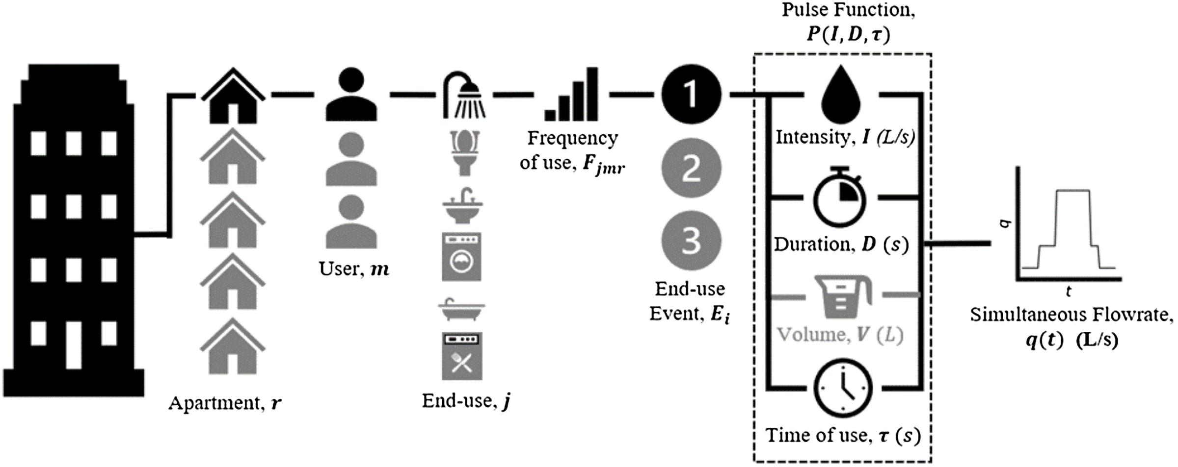
For each day of water use, the frequency of use , for end use and user in apartment is determined. For each end-use event , the intensity , duration , and time of use are established to define the pulse function . The pulse function [Eq. (2)] is equal to intensity () between the time domain to and equal to 0 (zero) during all other periods. The modeling process is repeated for each user and end-use. The summation is done for each apartment , for a building size at each second of the day . To develop aggregated data on simulated water usage, the modeling process was repeated for a specified number of days of total building water usage. More details of the parameters involved and temporal resolution, are presented in the following subsections.
Apartments,
The model is constructed to simulate a specific number of apartments from to . This is done by looping through each apartment, where the building simultaneous flow rate is the summation of each apartment’s flow rate at each time step . Washing machine, dishwasher, and bath use are simulated at an apartment level.
Users,
Shower, tap, and toilet end-use functions are modeled at a user level. The developed stochastic demand model aims to emulate water consumption ranging from zero to five users per apartment. REUS has shown that the number of household members is an important factor in the frequency of use for certain end uses. And as a result, per capita usage reduces as household occupancy increases because of the shared water consumption across taps, washing machines, and dishwashers.
End Uses,
In the present study, the term end use refers to a specific water-use group, i.e., showers, taps (faucets), toilets (water cisterns), washing machines, dishwashers, and baths, and is denoted by the index . As a result, . In this study, it was assumed all apartments feature each end use 100% of the time. Shower and bath end uses were modeled as single events. Toilet use considers both half- and full-flush events. In a practical setting, tap (faucet) use is performed across several household rooms and functions, i.e., hand washing after toilet use (bathroom), prerinsing/washing dishes (kitchen), or soaking clothes (laundry). Other studies have attempted to recreate these behaviors (Blokker et al. 2010; Ferreira and Goncalves 2020).
However, the statistical data presented in REUS do not always discriminate between the various functions and locale of taps within a specific household. Because of this, the model does not differentiate between the various functions of tap end use. Washing machine and dishwasher demand patterns are largely dependent on machine consumption and user-selected cycle functions (i.e., eco, fast wash, and so on). Although some studies have conducted user surveys to determine the frequency of cycle selection (Ghobadi 2013), there are no practical means to cross-correlate machine volume and cycle function from high-level REUS data. As a result, washing machine use assumed a typical wash cycle conducted over a 2-h period that includes four cycles (presoak, prewash, wash, and rinse). Similarly, dishwasher use assumed the total event volume consists of three cycles across 1.5 h.
Frequency of Use
The frequency of use is the total number of daily events for a specific end use, . First, the model determines the event frequency from an empirical PDF []. This is a noninteger value that is converted to an integer value. Then, to consider household occupancy, an occupancy event scaling function is applied to lower/increase the occurrence of end-use events.
Noninteger Values
Empirical PDFs produce noninteger values; however, the model cannot simulate a portion of an event, meaning an integer value is required. Simply rounding the noninteger value leads to an underestimation of events, and by extension, water consumption, for end uses that are infrequently used. Table 1 describes how the model handles noninteger values. The model first determines a noninteger value . The initial number of events is the integer of the selected number of events (). Then, the model conducts a single trial for an additional event to occur, where the probability for success is the initial noninteger value minus the initial number of events. If the trial is successful, the additional event is added to the initial number of events.
| Step | Formula | Example |
|---|---|---|
| Step 1. Select a noninteger value from an empirical PDF | ||
| Step 2. Determine the initial number of end-use events | ||
| Step 3. Determine the probability of success and failure | ||
| Step 4. Run an additional event trial | Success: | |
| Fail: | ||
| Step 5. Combine initial value and additional event trial | Success: | |
| Fail: |
Occupancy Event Scaling Function
REUS demonstrate daily per capita water consumption for taps, washing machines, dishwashers, and baths is influenced by household occupancy. The impact of occupancy is aligned with water consumption associated with washing activities, which is shared among household occupants. (shower and toilet per capita water consumption does not generally alter with a change in household occupancy). Much like Thyer et al. (2009), the model implements an occupancy event scaling function to raise or lower the occurrence of end-use events considering the total number of apartment users to influence per capita water consumption. Due to the high frequency of occurrence and user focus, shower, tap, and toilet frequencies are determined as events per capita per day (EPCD) [Eq. (3)]. Owing to the shared function and comparatively lower frequency of use, washing machine, dishwasher, and bath end-uses are selected as events per apartment per day (EPAD) [Eq. (4)]
(3)
(4)
Pulse Function
The pulse function is a combination of an end-use intensity , duration , and time of use . For toilets, washing machines, dishwashers and baths, a specific end-use event duration is calculated by end-use volume divided by intensity . As shown in Fig. 1, first the frequency of use, which is the total number of specific end-use events for user in apartment is determined from a PDF. Then, for each end-use event , end-use intensity, duration, and time of use are determined. Intensity and durations are derived from either a PDF or an assumed fixed value. Time of use is derived from a weighted PDF that reflects the average diurnal pattern for a specific end-use.
Intensity
Fixture intensity is a specific end-uses flow rate. Shower, tap, and bath intensity values are selected through developed empirical PDFs and are described by Eq. (5). For remaining fixtures, the intensity will be a fixed (uniform) value that is a predetermined fixture flow rate value [Eq. (6)]. This is because REUS results are volume focused for toilet, washing machine, dishwasher, and bath end-uses, and rarely present flow rate intensities
(5)
(6)
Duration
Duration for shower and tap end uses are defined by empirical PDFs based on statistical data from selected REUS [Eq. (7)]. Fixture duration for all remaining fixtures is a function of volume and intensity , shown in Eq. (8).
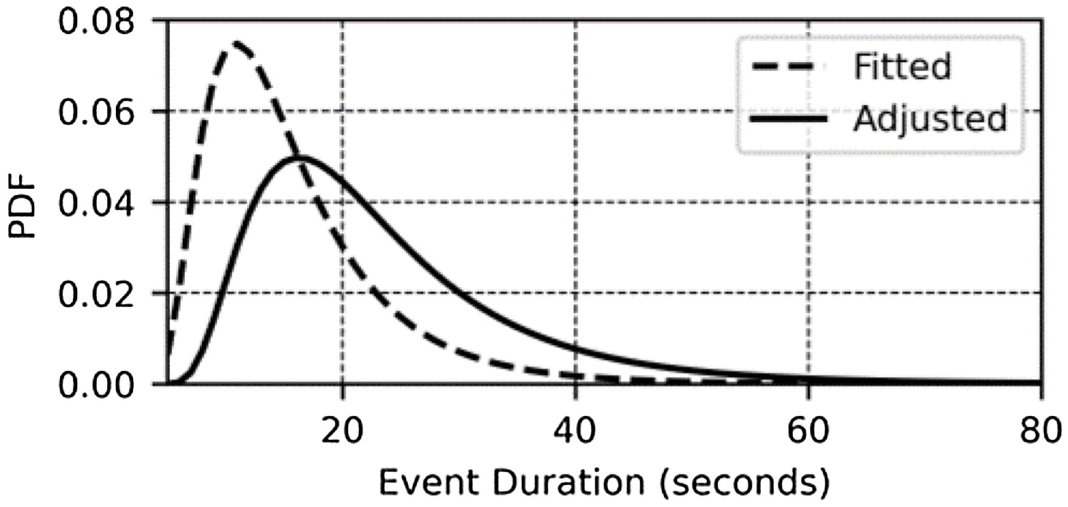
In REUS, relative frequency plots for tap use typically group events longer than 60 s into a single bin, giving little accuracy to tap durations beyond this time domain. In addition, there is a high degree of measurement uncertainties because REUS typically log flow rates at a frequency of 5 to 10 s. Redhead et al. (2013) explained that a tap event would be rounded to the next greatest logging interval, leading to an inflated value of the true event. To offset data set limitations, the duration is adjusted to better represent average water consumption volumes seen within selected REUS. The original fitted event duration is adjusted by a factor of (Fig. 2). This produces a probability function that subsequently increases or decreases end-use duration. Altered event durations will influence fixture -values because they are a function of time used
(7)
(8)
Volume
For shower and tap use, fixture volume is a product of duration and intensity , as in Eq. (9).
For volume-based fixtures (toilets, washing machines, dishwashers, and baths) total water consumption will be driven by fixture volumes selected from continuous distributions derived from selected REUS, as in Eq. (10)
(9)
(10)
Time of Use
To establish an event time of use, the model adopts a weighted PDF that represents the average water consumption (diurnal pattern) for each hour of the day. The probability of each hour varies, but overall, the weighted PDF satisfies the condition where the sum of all probabilities for each hour of the day is equal to 1. For the selected hour, the start time of each end-use event is randomized and assumes an equal probability for each second. The model adopts a diurnal pattern for each end use because specific water-use functions vary across a typical day of water consumption. All simulated apartments draw from the same pattern; however, because the event time of use is randomized based on a weighted probability, the hour of peak water consumption between each apartment is varied. REUS typically present a diurnal pattern that combines both weekday and weekend use. Because of this, the model does not differentiate between weekday and weekend water consumption.
Temporal Resolution
The temporal resolution needs to be decided, and it is not necessarily limited by the water demand sampling interval in the REUS. In this study, indoor end uses were modeled at an individual household user level at a temporal resolution of 1 s. Users can be grouped to describe either a single household or several households to emulate water consumption in a multilevel residential building.
Data Preparation
In the following subsections, the process to prepare REUS statistical information for parametrization is described.
Step 1: Gather Required REUS Data
For each selected REUS study from a specific country/region, presented data need to be evaluated to determine its suitability for model parameterization. A worldwide review by Mazzoni et al. (2023) has categorized REUS results into six specific levels of detail (L1–L6). Each level is representative of the depth of analysis conducted. Some or all elements of L1 to L5 REUS data are required to develop the necessary inputs for the stochastic water demand model (Table 2). L1 and L2 are used to understand average water-use characteristics and serve as a reference to validate the stochastic water demand model. End-use statistical parameters categorized as L3 are required to develop the empirical PDFs for model inputs’ frequency of use, intensity, duration, and volume where required. Diurnal end-use patterns are used to derive the time-of-use inputs categorized as L4. L5 data are used to consider the influence of household occupancy for specific end uses.
| Level | Description | Demand model inputs |
|---|---|---|
| L1 | Daily per capita end-use water consumption | Understand water consumption and model validation |
| L2 | End-use parameters (average values) | Understand water consumption and model validation |
| L3 | End-use statistical parameter distribution | Model inputs: frequency of use, intensity, duration, and volume |
| L4 | Daily end-use profiles | Model inputs: time of use |
| L5 | Determinants of end-use water consumption and parameters | Model inputs: occupancy event scaling factors |
| L6 | Efficiency and diffusion of water-saving end uses | Not required |
Source: Data from Mazzoni et al. (2023).
Step 2: Define Model Inputs and Assumptions
Known end-user statistical information is collated, and assumptions are needed for model implementation. Table 3 presents typical statistical parameters presented within global REUS for each end use. For shower and tap use, the required model inputs are more readily retrieved from end-user statistical information presented in REUS in the form of weighted or fitted empirical PDFs. For the remaining end-uses, (toilet, washing machine, dishwasher, and baths), results presented in REUS have a stronger focus toward volume per event. Mazzoni et al. (2023) have shown only a small number of REUS present the flow rate (intensity) and duration of use for these end uses. Because of this, missing statistical information needs to be offset by other available end-use statistical parameters or assumed values. End uses with no statistical information regarding duration are supplemented by a function of volume divided by intensity. When end-use intensity is unknown, an assumed value taken from end-use specific data is used.
| Model inputs | End-use | |||||
|---|---|---|---|---|---|---|
| Shower | Tap | Toilet | WM | DW | Bath | |
| Frequency of use, | ||||||
| Duration, | ||||||
| Intensity, | AV | AV | AV | AV, PDF | ||
| Volume, | ||||||
| Time of use, | ||||||
| Scaling factor, | FF | FF | FF | FF | FF | FF |
| Simultaneous operation | Yes | Yes | Yes | No | No | Yes |
| Modeling level | User | User | User | Apt | Apt | Apt |
| Frequency of occurrence (%) | 100 | 100 | 100 | 100 | 100 | 100 |
| Number of pulses per event | 1 | 1 | 1 | 4 | 3 | 1 |
| Duration of event (h) | — | — | — | 2 | 1.5 | — |
Note: WM = washing machine; DW = dishwasher; PDF = probability density function; AV = assumed value; FF = fitted function; and Apt = apartment.
REUS statistical parameters need to be reorganized into comparable units concerning each end use and model input (frequency, intensity, duration, volume, and time of use). The developed model simulates water consumption on a user level (per capita/per day) for shower, tap, and toilet end uses; in contrast, owing to their collective use, washing machine, dishwasher, and bath use is modeled at an apartment level (per apartment/per day). Where required, REUS results presented in the unit of per household are divided by the respective study’s average number of household occupants to convert to a per capita basis. Values presented in a weekly format are divided by 7 days to obtain a daily value.
Assumptions should be made to consider the number of simultaneous operations of the same end use within each apartment. In the current study, there was no limit to the number of simultaneous end-use operations for showers, taps, toilets, and bath end-uses. This was done to (1) impose a greater demand on a specific plumbing system, and (2) it is not always possible to accurately determine the number of end-use points for specific REUS households. Simultaneous operation was prevented for washing machine and dishwashing end uses because it is unlikely more than one washing machine/dishwasher would exist in a typical household or apartment.
Model Parameterization
The methods used to fit end-use statistical parameters to develop empirical PDFs for model functions (frequency of use , intensity , duration , and volume ) are presented. Then, the procedure for determining the time of use is then outlined. Lastly, the process to determine occupancy scaling functions is described.
End-Use Empirical Probability Density Functions
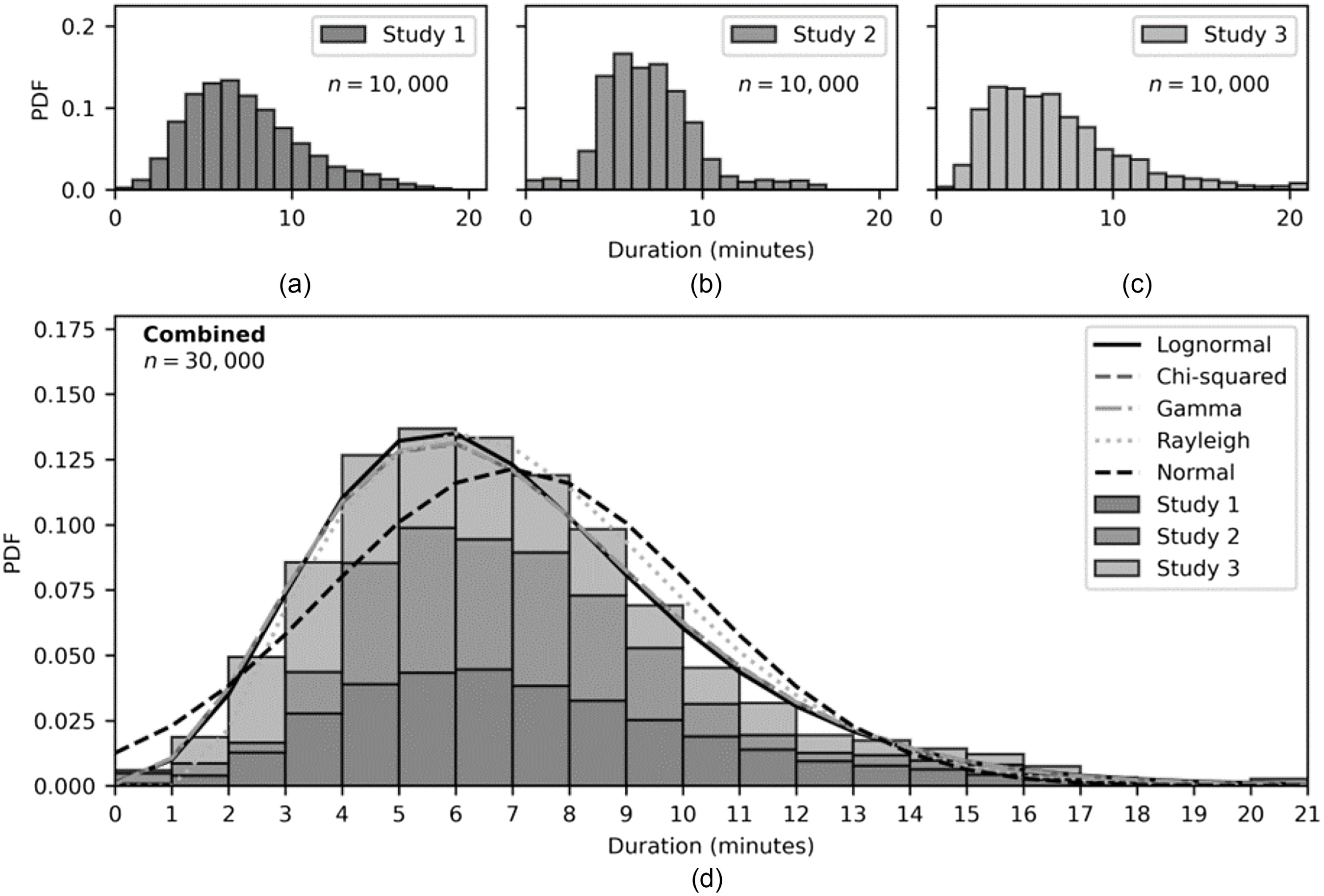
The process to develop empirical PDFs is completed in three steps: (1) simulation of individual REUS characteristics, (2) combining similar data sets, and (3) fitting combined data sets to select a suitable empirical PDF. The following section outlines a methodology to generate an empirical PDF that is representative of multiple REUS, allowing for an increased sample size of water-use behavior for a specific country or region. An example using three selected REUS to estimate duration for the shower end use is presented (Fig. 3).
Step 1: Simulate Individual Data Sets
For each selected REUS, end-use statistical parameters are used to simulate individual data sets to form the basis of data to be fitted against selected continuous PDFs. Each simulated data set assumes a weighted probability distribution that is representative of the specified end-use statistical parameters and 10,000 trials () [Figs. 3(a–c)].
Step 2: Combine Data Sets
For each end-use, individual simulated data sets for the same end-use input (frequency, duration, intensity, and volume) are then combined into a single array to produce the combined end-use data set to be fitted for an empirical PDF. Fig. 3(d) presents a stacked histogram containing each simulated data set. The total height represents the combined data set () for shower duration from three different REUS.
Step 3: Fit Empirical Probability Density Function
Like Mazzoni et al. (2023), combined data sets are fitted against continuous probability density functions. Fitting is done using a statistical module within data analysis packages, i.e., MATLAB or Python. The combined array assumes a discrete number (bins) for frequency of use, duration, intensity, or volumes. The probability density function that produces the lowest sum squared error is selected as the empirical PDF. The shape, location, and scale parameters for the selected distributions are then extracted for use in the water demand model. Fig. 3(d) presents five continuous probability distributions that produced the lowest sum squared error for the combined data set for shower duration in minutes.
Weighted PDF for Fixture Time of Use
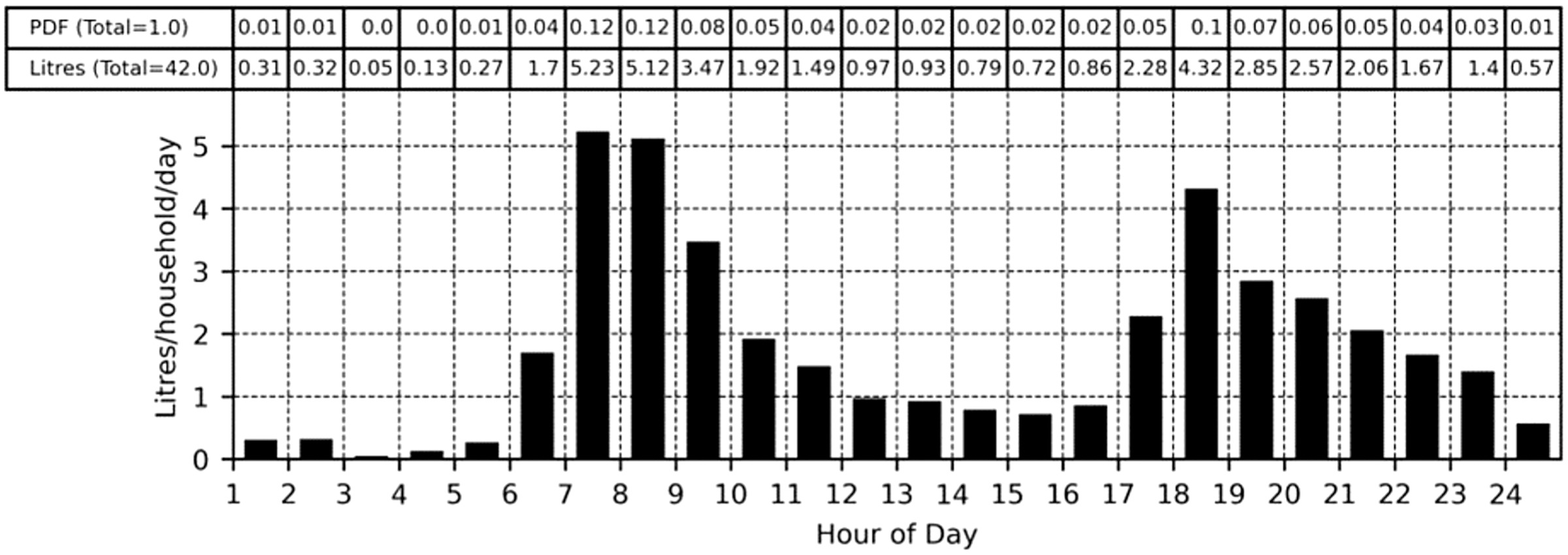
Weighted PDFs are derived by normalizing hourly diurnal water consumption patterns retrieved from selected REUS for each end use. Normalizing is completed by taking the sum of average water consumption for all hours of the day and dividing it by each respective hour’s water consumption (Fig. 4). This process is repeated for each end use across all selected diurnal patterns. The resulting time-of-use weighted probability density value for each hour of the day is the average value of all normalized diurnal patterns for each specific end-use.
Occupancy Event Scaling Function
The model implements an occupancy event scaling function to raise or lower the occurrence of per capita water consumption as a function of the total number of apartment users. Occupancy event scaling functions are developed by fitting the average values of the formula presented in selected REUS. Relationships between apartment occupancy and event scaling can be either linear or nonlinear and are end-use-specific. The function baseline () was set at a value representing the combined average occupancy of all the selected REUS, i.e., the closest interpretation of per capita per-day water use.
Determination of Fixture -Values
This section details how the probability of fixture use (-values) is determined from the stochastic water demand model.
Peak Demand Design Formula
A recognized plumbing design formula is the MWM proposed by Buchberger et al. (2017) [Eq. (11)]. The zero-truncated binomial distribution is an adaptation of the formula proposed by Wistort (1994) for describing fixture water-use behavior. The MWM considers the intermittent flow of plumbing systems, specifically for buildings with smaller sizes that spend a considerable amount of time at zero demand or stagnation conditionswhere = 99th percentile flow rate; = probability of stagnation; = index for fixture groups associated with an end use, i.e., kitchen taps, laundry taps, basins, and so on; = total number of fixtures groups along a downstream pipe; = number of fixtures for a specific fixture group downstream of a pipework section; = specific fixture flow rate; = probability of fixture use (probability that a fixture group is running water during the peak period); and th percentile of the standard normal distribution, approximated as 2.326. The formula reduces to Wistort’s original formula (Wistort 1994) once the probability of stagnation reaches zero [Eq. (12)].
(11)
(12)
The probability of fixture use (-values) forms key information needed. The values can be country-specific, and they are unknown for water use outside the US. The current study intends to provide recommended probability values of fixture use (i.e., -values in the modified Wistort method) for common indoor fixtures for a specific country or water-use region, considering both the effects of building size and occupancy.
Basic Formula
The methodology to determine the probability of fixture use during the peak hour of water consumption () is adapted from the process presented by Buchberger et al. (2017) and Omaghomi et al. (2020). Eq. (13) describes an end-uses probability of use during the hour of greatest water consumption for a single day of water consumption. Using the developed stochastic water demand model, for a building with a specified size , individual apartment water consumption is simulated for a specified number of total building occupants . For each day , of simulated water use, the hour of greatest water consumption (volume) is identified. During this hour, the total time a specific end use is operational is recorded for each apartment from 1 to . The cumulative time of a fixture group is then divided by the total observational time , which is defined as the product of 3,600 s (1 h) and the total number of observed apartments . This procedure is repeated for the number of days required for each fixture’s -value to reach convergence, where the cumulative -values from the previous 20 days of water use impose a change less than 0.001 for all end uses, as defined in Eq. (14). The double asterisk over denotes the summation of all similar processes, i.e., all end uses.
The proposed methodology differs from the previous studies in one key aspect. The previous work used original water end-use data, and as a result, it was able to define the number of end-use (fixture) points of use in each monitored household. This end-use (fixture) quantity was considered in the total observational time and subsequently increased the cumulative observational time by a factor of the number of known end-use (fixture) points in each observed household, i.e., would double for two end-use (fixture) points of the same end use, would triple for three end-use (fixture) points of the same end use, and so on. By considering the number of end-use (fixture) points, the previous methodology calculated the probability of use for an individual end-use (fixture) point.
The present study’s methodology removes the requirement of known end-use fixture quantities by calculating the probability of use for each end use as a whole group. The increased probability values are then managed through the consideration of building occupancy, explained in further detail under the “Implementation of Fixture p-Values in Plumbing Design Formula” section
(13)
(14)
Effects of Building Size and Building Occupancy
Omaghomi et al. (2020) demonstrated that fixture -values (probability of use) are a function of both building size and occupancy. As apartment occupancy, and by extension building occupancy increases, typically so does the total operational time of plumbing fixtures. Additionally, as building size increases by the number of apartments, the average fixture -value diminishes and begins to stabilize, reaching an almost constant value when over approximately 20 apartments (for a given occupancy rate). The diminishing -value is attributed to the increasing randomness of water-use events as additional water users are considered.
In the current study, the dependency of fixture -values on occupancy and building size was determined by simulations. Water consumption for buildings ranging from 1 to 20 apartments with occupancy levels equal to (one occupant per apartment) to (four occupants per apartment + one) was simulated. Simulations allow for the model to randomly select between zero and five occupants (users, to 5) per apartment until the sum of occupants from each apartment equals the required occupancy level for the building. The -values for each fixture were recorded and indexed in a matrix .
Implementation of Fixture -Values in Plumbing Design Formula
The proposed implementation of fixture -values considers the number of building apartments and the total number of occupants downstream of a specific pipe section [Eq. (15)]. Fig. 5 demonstrates how a fixture’s -value is calculated over a two-step process. Step 1 is to calculate the baseline fixture -value as a function of building size [Eq. (16)]. Step 2 is to determine the increase of baseline fixture -value by an occupancy factor , that is specific to the building’s size (number of apartments) [Eq. (17)].
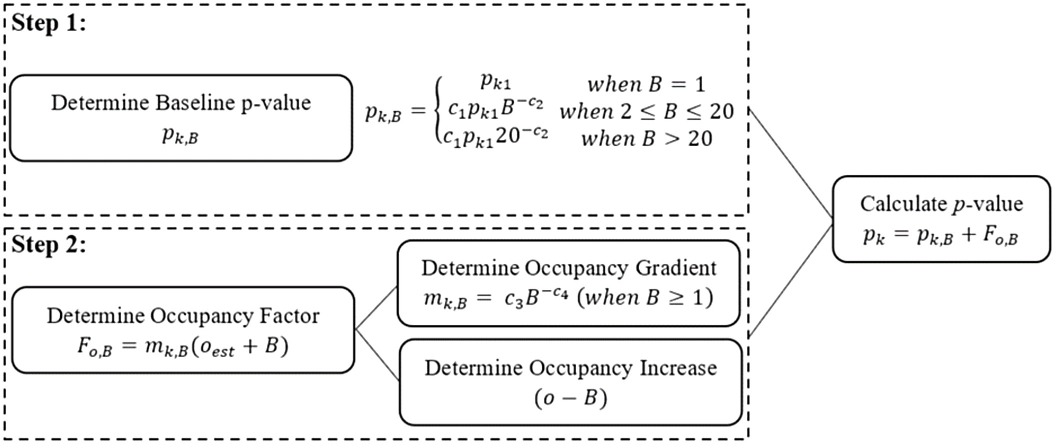
The baseline -value assumes an average building occupancy of one person per apartment (). Coefficients and are determined for each fixture end use by fitting a nonlinear equation using modeled -values for buildings ranging in size from 1 to 20 apartments in the form of Eq. (16). The term represents the probability of fixture use for a single household. Like Omaghomi et al. (2020), it was assumed that -values have reached a steady state when a building size reaches 20 apartments or greater.
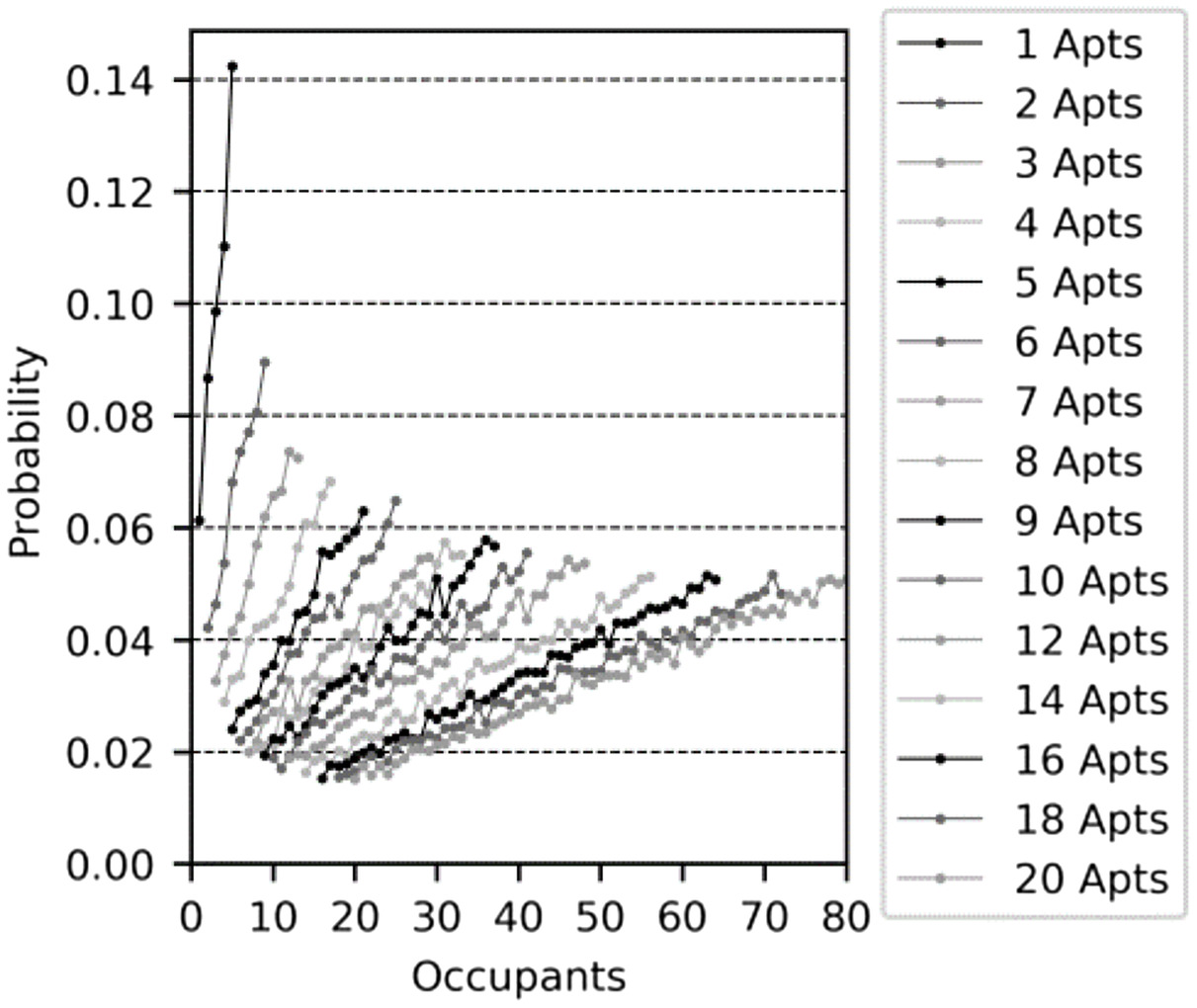
The occupancy factor increases the baseline fixture -value by the product of building occupants greater than [i.e., ] and the occupancy gradient [Eq. (18)]. Fig. 6 presents the typical relationship building size and occupancy has toward modeled fixture -values. Demonstrating for the same building size, an increase in occupancy leads to an increased -value because of additional fixture events during the peak hour of consumption. The occupancy gradient assumes a linear relationship between the minimum and maximum simulated -values for a building’s occupancy between to () for a specific number of apartments within a building.
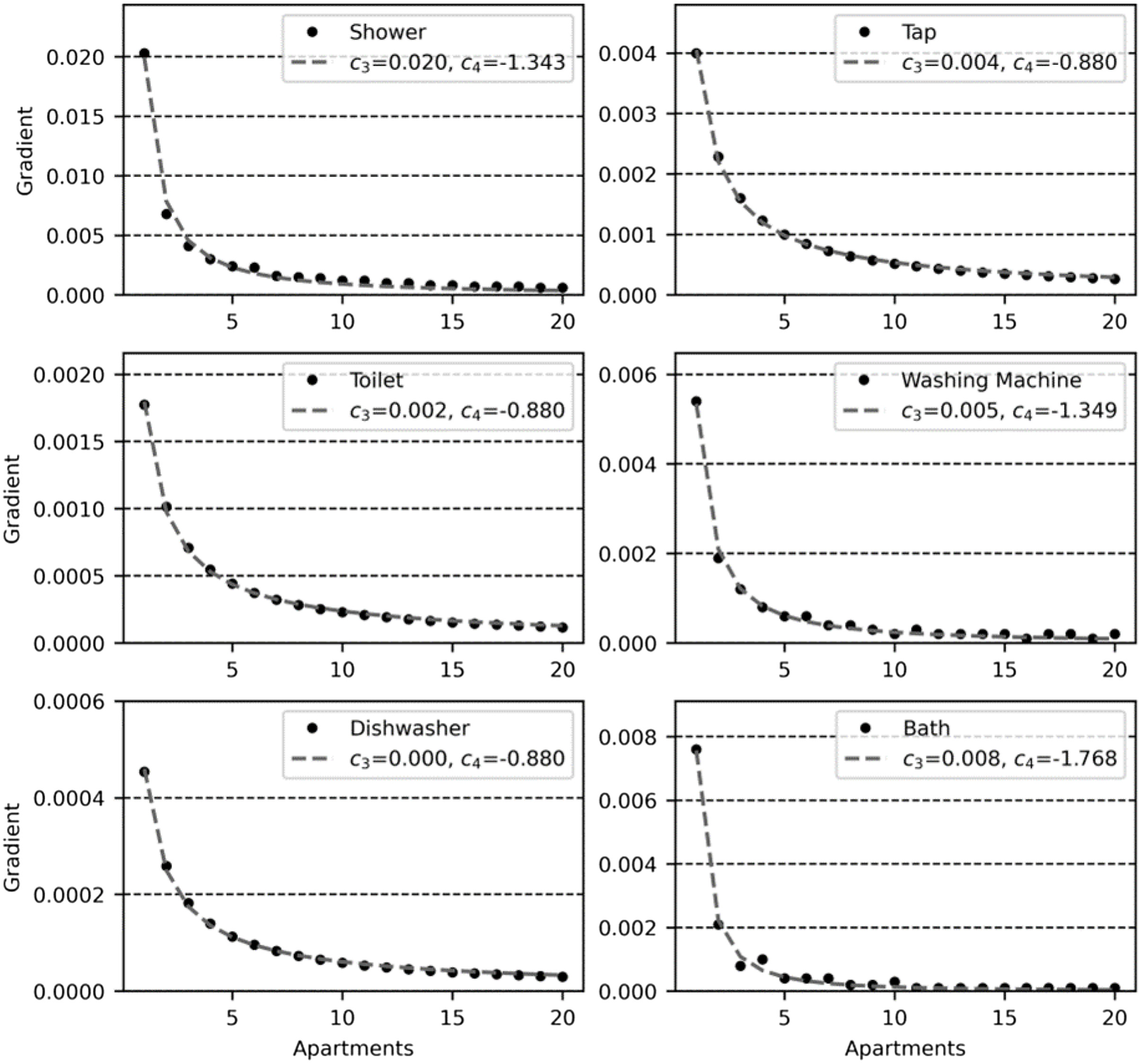
Using simulated -values for each building size from to 20 apartments, over the specified range of occupancy for each end-use, as shown in Fig. 6, the calculated occupancy gradient was calculated as a function of building size. Coefficients and as in Eq. (18) are determined by fitting plotted occupancy gradient values assuming a power law. From a practical perspective, hydraulic designers are supplied with a floor plan of building and apartment layouts; thus, it is expected the number of occupants can be estimated by the number of bedrooms in an apartment,
(15)
(16)
(17)
(18)
Results and Discussion
Stochastic Water Demand Model
This section details the selected REUS studies and determined end-use model parameters: frequency of use, intensity, duration, volume, time of use, and event scaling functions. Average simulated water consumption for each end use at an apartment level is presented and compared with selected REUS.
Australian Residential End-Use Studies
Table 4 presents a summary of the selected REUS used to develop the stochastic water demand model in this study. Five Australian REUS were used to demonstrate the process of the proposed approach for developing the stochastic water demand model, which should also work on similar REUS from other regions. With the use of digital (smart) water meters and disaggregation software, the combined studies characterized the water consumption of 1,062 total households and an estimated 3,169 occupants, with an average occupancy of 2.98 people per household. From this data, the selected study reports present end-use statistical parameters associated with each end-use characteristic (frequency, intensity, duration, volume, and time of use). Across the five studies, the average water consumption was 116.2 litres per capita per day (LPCD). In Australia, shower use tends to dominate overall water consumption, accounting for almost 35% of water consumption, followed by tap, toilet, and washing machine use at approximately 19%–21% of total water consumption. The remaining 5% of water consumption is shared between dishwasher and bath use.
| Study (reference) | Study households | Study participants | Average water consumption (LPCD) |
|---|---|---|---|
| Yarra Valley, VIC (Roberts 2005) | 100 | 324 | 153.5 |
| Southeast QLD (Beal and Stewart 2011) | 252 | 655 | 129.2 |
| Melbourne, VIC: winter (Redhead et al. 2013) | 300 | 930 | 98.8 |
| Melbourne, VIC: summer (Redhead et al. 2013) | 300 | 930 | 108.8 |
| City West Water, VIC (Siriwardene 2019) | 110 | 330 | 123.9 |
| Average | 2.98 | 116.2 | |
Model Parameterization
End-Use Empirical Probability Density Functions
Table 5 presents the developed empirical PDFs and assumptions used in the developed stochastic water demand model. Fitted distributions were derived using Python’s fitter module (Cokelar 2019). Distributions were fitted against the module’s 10 common distributions: Cauchy, chi-squared, exponential, exponential power, gamma, lognormal, normal, power law, Rayleigh, and uniform. Of the evaluated distributions, the most frequently occurring distributions that led to the lowest sum squared error for fitted data sets were the lognormal and normal distributions. The less common fitted PDFs were Cauchy, chi-squared, exponential, gamma, and Rayleigh. The higher occurrence of the lognormal distribution is consistent with the most common end-use empirical distribution presented in the supplementary data of Mazzoni et al. (2023) that considered exponential, gamma, lognormal, normal, and Weibull PDFs.
| Fixture | Duration, | Frequency of use, | Intensity, | Volume, | ||||
|---|---|---|---|---|---|---|---|---|
| Distribution | Parameters | Distribution | Parameters | Distribution | Parameters | Distribution | Parameters | |
| Shower | Lognormala,b,c,d,e,h | , , | Normala,b,c,d,e,f | , | Lognormala,b,c,d,e,i | , , | Uniform | |
| Tap | Lognormala,c,d,e,j | , , | Rayleigha,c,d,e,f | , | Lognormala,c,d,e,i | , , | Uniform | |
| Toilet (half-flush) | Uniform | Chi-squareda,b,c,d,e,f,m | , , | Uniform | k | Normalb,c,d,e,n | , | |
| Toilet (full flush) | Uniform | Lognormala,b,c,d,e,f,l | , , | Uniform | k | Normalb,c,d,e,m | , | |
| Washing machine | Uniform | (four cycles over 2 h) | Lognormala,b,c,d,e,g | , , | Uniform | k | Gammaa,b,c,d,e,n | , , |
| Dishwasher | Uniform | (three cycles over 1.5 h) | Lognormala,b,c,d,e,g | , , | Uniform | k | Lognormala,b,c,d,e | , , |
| Bath | Uniform | Exponentiala,b,c,d,e,g | , | Cauchyb,e,i | , | Lognormalb,c,d,e | , , | |
Note: s = shape; loc = location; and scale = scale.
a
Roberts (2005) data used to develop distribution.
b
Beal and Stewart (2011) data used to develop distribution.
c
Redhead et al. (2013)’s winter data used to develop distribution.
d
Redhead et al. (2013)’s summer data used to develop distribution.
e
Siriwardene (2019) data used to develop distribution.
f
Events per capita per day.
g
Events per household per week.
h
Duration (min).
i
Flow rates ().
j
Most studies reported a mean tap event duration of 18–26 s; however, upon recreation of relative frequency plots, the mean was underestimated, so an adjustment factor of 1.5 was applied to the model.
k
Flow rates retrieved from IAPMO Water Demand Calculator (IAPMO 2020).
l
Beal and Stewart (2011) displayed relative frequency plots for both full and half-flush toilet events per household; all other studies displayed relative frequency plots for total flushes per capita per day. These values were then diversified between the average ratio of half-flushes and full flushes for each study.
m
n
Four studies presented washing machine volumes with front- and top-loader values combined. Siriwardene (2019) split washing machines volumes, and data sets were weighted based on appliance stock: 53% front loader, and 47% top loader.
The fixed intensity values displayed in Table 5 were taken from the IAPMO Water Demand Calculator (IAPMO 2020). The upper-limit flow rate was used to impose a greater demand on simulated plumbing systems. Values presented in the IAPMO Water Demand Calculator are a result of flow rate evaluation presented by Buchberger et al. (2017); it was assumed that Australian plumbing systems use similar products.
End-Use Time of Use
The dashed lines shown in Fig. 7 are the weighted probability distributions (diurnal patterns) determined for each end use. Box plots for each end use and hour present the variance between eight selected diurnal patterns used to determine the weighted probability distributions. The selected diurnal patterns represented the average water consumption profile for the specific study’s monitoring period. As a rule, each end use has two distinct peak periods occurring in the morning and evening. Shower, washing machine, and toilet end uses have sharper morning peaks. Conversely, dishwashing and bath end uses have greater consumption during the evening. Tap peak periods can be described as similar between morning and evening periods.
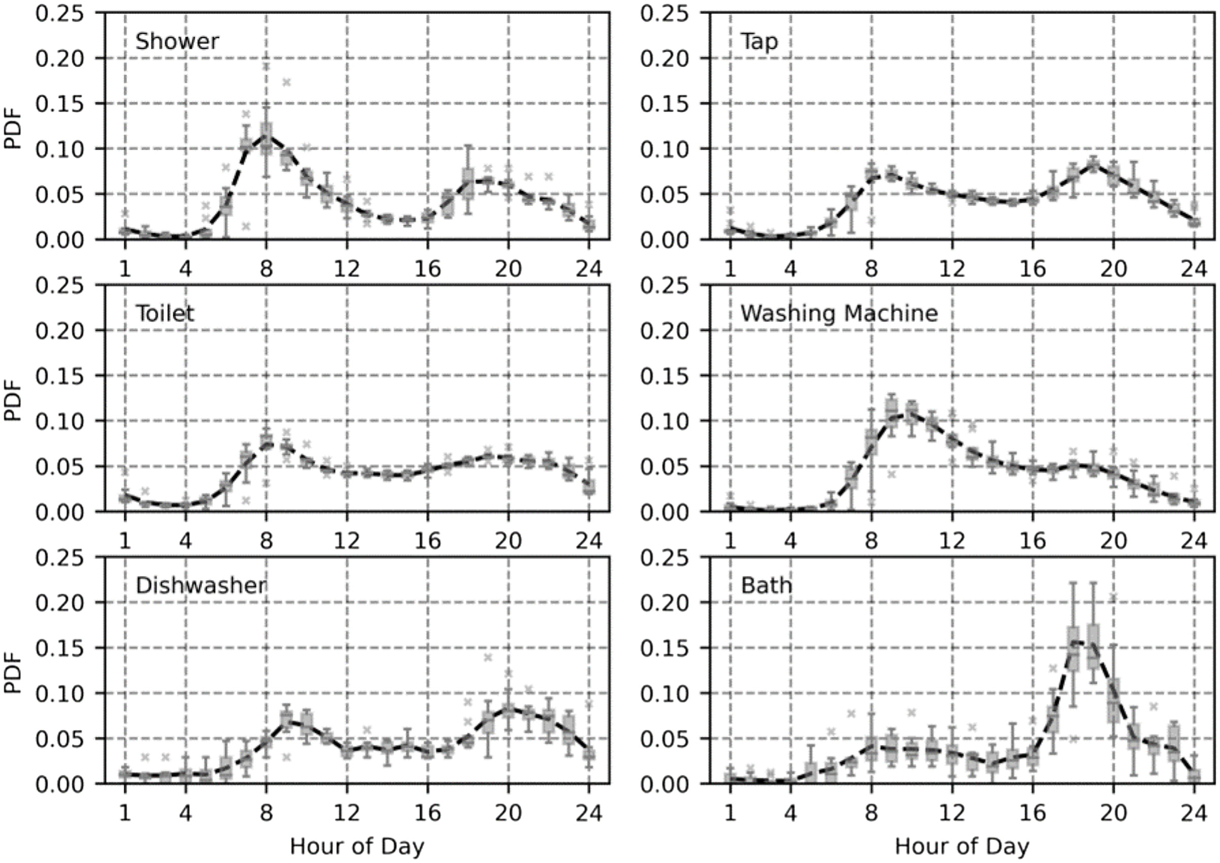
REUS typically present a diurnal profile that combines both weekday and weekend use. The selected RUES varied between winter and summer monitoring periods, offering a diversified profile that is representative of water use across different Australian climates. In the current study, weekday patterns were selected over weekend patterns to maintain consistency with combined (weekday and weekend) patterns because weekday use represents more typical water-use behavior, i.e., 5 out of 7 days of the week. Omaghomi et al. (2020) demonstrated for all fixtures excluding showers, weekend -values are comparable to or greater than weekday -values. Also, there was a statistically significant increase in bath, washing machine, and tap use on weekends compared with weekdays. This identifies future models that can be improved upon to consider both weekday and weekend use. Moreover, data on the frequency of use for end uses comparing weekend and weekday use is scarce.
Occupancy Event Scaling Function
Table 6 displays the developed occupancy event scaling functions determined by fitting the average values of the occupancy-related formula presented by Roberts (2005), Redhead et al. (2013), and Siriwardene (2019) for tap, washing machine, dishwasher, and bath use. Shower and toilet use do not normally vary because of occupancy; therefore, for all levels of apartment occupancy. For tap use, the studies have shown that daily per capita tap consumption decreases with an increase in household occupancy; the fitted function follows a power law. Conversely, the frequency of household washing machine, dishwasher, and bath events increases with occupancy. The event scaling function for washing machines is linear, dishwashers follow a power law, and bath use was assumed to be a linear function of occupancy.
| End use | Fitted function |
|---|---|
| Shower | |
| Tap | |
| Toilet | |
| Washing machine | |
| Dishwasher | |
| Bath |
Average Water Consumption
To demonstrate the suitability of the developed water demand model, the following section will present modeled water consumption data compared with the selected REUS average water consumption values.
Fig. 8 presents modeled per capita water use for six indoor fixture groups and total apartment consumption for single households. The modeled apartment structure assumes three occupants and 1,000 simulated days of water use. The solid line across the box plot represents the median value, the dashed line corresponds with the average value and for comparison, and the average water consumption from selected REUS is shown as the solid dot symbols. The developed model shows good agreement for shower, tap, toilet, and washing machines, with only a small amount of underestimation of 5.5%, 7.3%, 7.8%, and 1.6%, respectively.
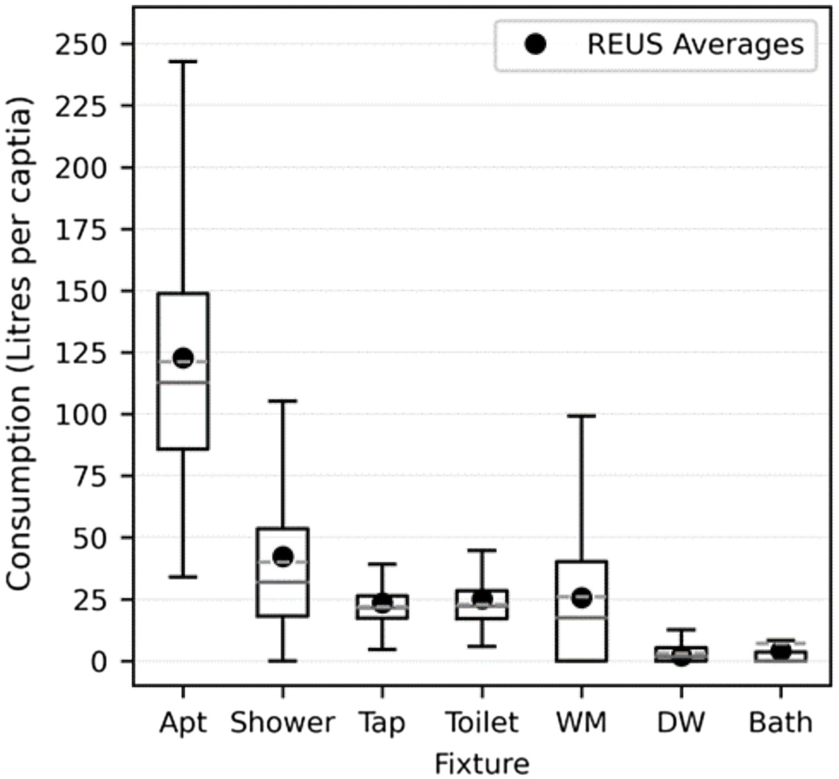
The developed model showed an overestimation of dishwasher and bath use. This is because the model assumed that baths and dishwashers are present in 100% of apartments, where typically, not all household feature these end uses in selected REUS. The relative discrepancy is high due to the small base value; however, the absolute discrepancy is small, and they do not affect the overall performance as indicated by the total apartment consumption.
Fixture -Values and Occupancy Gradient
The resulting fixture -value and occupancy gradient functions used for plumbing design formula are presented in Table 7. Presented in Fig. 9 are modeled baseline fixture -values (dots) and fitted functions (dashed lines). All modeled end uses display a positive correlation between occupancy and -values. Furthermore, the increase each occupant imposes on the -value reduces with an increase in building size, i.e., the gradient begins to flatten as building size increases. For tap, toilet, and dishwasher end uses, excluding a jump between one and two apartments, building size had little influence on modeled -values. These end uses contribute to a small percentage of peak-hour water use that is typically dominated by shower and washing machine end uses.
| Fixture | probability | occupancy | |||
|---|---|---|---|---|---|
| Shower | 0.061 | 0.966 | 0.992 | ||
| Tap | 0.009 | 0.009 | — | 0.999 | |
| Toilet | 0.002 | 0.002 | — | 0.999 | |
| Washing machine | 0.031 | 0.956 | 0.996 | ||
| Dishwasher | 0.001 | 0.001 | — | 0.999 | |
| Bath | 0.006 | 0.557 | 0.994 |
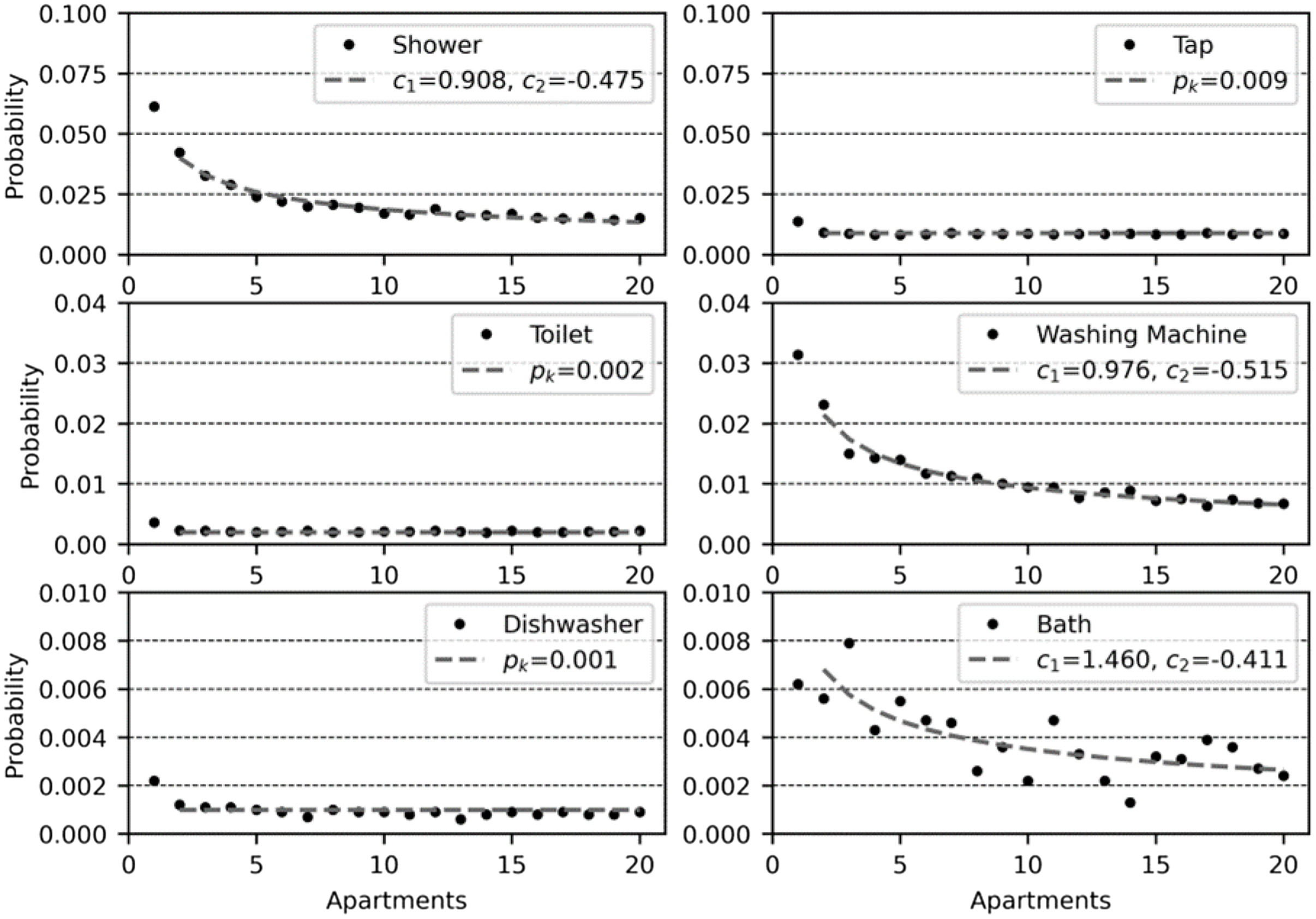
Due to the small differences, baseline fixture -values were fixed, regardless of building size. Fixed -values were determined by taking the average of all minimum -values modeled for a building ranging from 1 to 20 apartments. Bath use displayed a weak correlation between occupancy and peak-hour water consumption. This is likely due to the low frequency of use coupled with a peak consumption period that occurs in the evening, which is outside the morning peak periods of shower and washing machine use.
Shown in Fig. 10 are occupancy gradient values () fitted as function of building size assuming a power law [Eq. (18)]. Results demonstrate that occupancy has a greater influence on a per capita basis for smaller building sizes ranging from 1 to 10 apartments.
Validation of -Values
To assess the accuracy of the developed methodology, the design flow rates of four buildings presented by Josey et al. (2023) were estimated and then compared with measured peak flow rate observations. Also considered were the 99th percentile flow rates of 30 days of simulated water consumption using the develop stochastic water demand model considering building size and number of occupants.
The monitored buildings form part of an ongoing water demand investigation conducted by the Hydraulics Consultant Association of Australia (HCAA) (HCAA 2019). Fixture flow rates assumed nominal values presented in AS/NZS 3500.1:2021 (Standards Australia 2021), and the number of building occupants was estimated by the total number of bedrooms plus one occupant for all apartments within each building. Fig. 11 displays the estimated flow rates using the developed -values and proposed method that implements determined -values in the MWM. These values were compared against the observed 99th percentile nonzero flow rate (observed during the single peak hour of water consumption) and design flow rates estimated by the current Australian plumbing standard [AS/NZS 3500.1:2021 (Standards Australia 2021)].
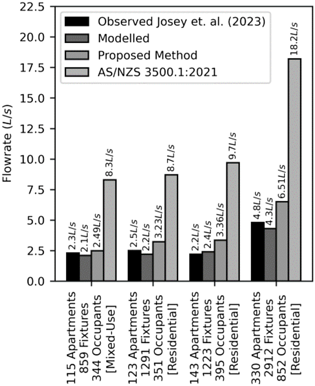
The estimated flow rates using the developed method showed a reasonable agreement with observed values. Estimated values were between 7% and 36% greater than the observed 99th percentile flow rates. It is hypothesized that a degree of overestimation is preferred because pipe frictional losses, for the same change in flow, are greater for smaller pipe sizes. The proposed formula offers a significant improvement over the current Australian standard, reducing demand estimates by the current Australian plumbing standard by more than 250%. As building size increases, the estimated 99th percentile flow rates determined by the proposed methodology increasingly drifted apart when compared with modeled 99th percentile flow rates. This gap between estimated and modeled flow rates is aligned to the implementation of fixed baseline -values at a building size of 20 apartments or larger. In practice, these -values continue to diminish. The decision to fix -values at 20 apartments follows the convention presented by Omaghomi et al. (2020) and offers a factor of safety from a premise plumbing design perspective. The assumed occupancy levels for modeling had good agreement with 99th percentile flow rates within 5%–15% of observed values.
Conclusions
A new framework for estimating the fixture-use probability for peak water demand design in multilevel residential buildings has been developed and validated. The framework includes a new approach to develop a stochastic water demand model using only the high-level water end-use statistics extracted from published water end-use studies. Based on the developed water demand model, formulas to estimate a fixture’s probability of use have been developed. The formula presented in the current study considered both building size and the number of building occupants drawing water from a specific piped section. In this new framework, detailed household water-use information, such as the number of fixtures and number of occupants in each household, is not required. This makes the proposed new approach easier to implement than existing ones because the raw household water-use information is difficult to obtain due to privacy concerns and, even if available, data processing is time-consuming. The consideration of both building size and occupancy level provides practitioners with a practical approach to adjusting the fixture-use probability values for different design projects.
The probability of fixture use (-values) for Australian apartment buildings has been determined using the proposed new framework. These values have been used to estimate the peak water demand for four Australian buildings (three residential and one mixed-use). The estimated peak water demand values have been compared with observed water consumption data for the four buildings. The estimated peak flow rates were 7%–36% greater than the observed peak flow rates, and they are 29%–37% of the flow rates as would be designed using the current Australian cold-water plumbing standard AS/NZS 3500.1:2021 (Standards Australia 2021). The results demonstrate that the newly determined -values are representative of the actual water-use characteristics in Australian multilevel residential buildings, and they have enabled a significant improvement in the accuracy of peak demand estimation for plumbing system design. This validates the whole systematic approach for determining fixture -values, which is transferable to other countries. The presented probability of fixture-use values can be directly used by practitioners to design water supply systems for multilevel residential buildings in Australia. This information is also useful for future studies on the difference in fixture-use characteristics considering different countries and regions.
Data Availability Statement
The water usage database used in this study was provided by the Hydraulic Consultants Association of Australasia through the Water Demand Investigation project (https://www.waterdemand.com.au/). Data are available from the corresponding author upon request.
Acknowledgments
The authors thank the Hydraulic Consultants Association of Australasia for their support in the field investigation and the supply of water usage data. The first author thanks the Hydraulic Consultants Association of Australasia for contributing to the Ph.D. scholarship.
References
Arbon, N., M. Thyer, D. H. MacDonald, K. Beverley, and M. Lambert. 2014. Understanding and predicting household water use for Adelaide. Adelaide, Australia: Goyder Institute for Water Research.
AWWA (American Water Works Association). 2014. M22–manual of water supply practices: Sizing water service lines and meters. Denver: AWWA.
Beal, C., and R. A. Stewart. 2011. South East Queensland residential end use study: Final report. Brisbane, Australia: Urban Water Security Research Alliance.
Blokker, E., C. Agudelo-Vera, A. Moerman, P. Thienen, and I. Pieterse-Quirijns. 2017. “Review of applications for SIMDEUM, a stochastic drinking water demand model with a small temporal and spatial scale.” Drinking Water Eng. Sci. 10 (1): 1–12. https://doi.org/10.5194/dwes-10-1-2017.
Blokker, E., J. Vreeburg, and J. Dijk. 2010. “Simulating residential water demand with a stochastic end-use model.” J. Water Resour. Plann. Manage. 136 (1): 19–26. https://doi.org/10.1061/(ASCE)WR.1943-5452.0000002.
Buchberger, S., T. Omaghomi, T. Wolfe, J. Hewitt, and D. Cole. 2017. Peak water demand study: Probability estimates for efficient fixtures in single and multi-family residential buildings. Ontario, CA: International Association of Plumbing and Mechanical Officials.
Cokelar, T. 2019. “FITTER documentation.” Accessed February 9, 2023. https://fitter.readthedocs.io/en/latest/#.
DeOreo, W. B., P. W. Mayer, B. Dziegielewski, and J. Kiefer. 2016. Residential end uses of water, version 2. Denver: Water Research Foundation.
Douglas, C., S. Buchberger, and P. Mayer. 2019. “Systematic oversizing of service lines and water meters.” AWWA Water Sci. 1 (6): e1165. https://doi.org/10.1002/aws2.1165.
Ferreira, T. D. V., and O. M. Goncalves. 2020. “Stochastic simulation model of water demand in residential buildings.” Build. Serv. Eng. Res. Technol. 41 (5): 544–560. https://doi.org/10.1177/0143624419896248.
Ghobadi, C. 2013. Water appliance stock survey and usage pattern Melbourne 2012. Melbourne, Australia: Smart Water Fund.
HCAA (Hydraulics Consultants Association of Australasia). 2019. “Water demand investigation.” Accessed October 6, 2019. https://www.waterdemand.com.au/.
Hobbs, I., M. Anda, and P. A. Bahri. 2019. “Estimating peak water demand: Literature review of current standing and research challenges.” Results Eng. 4 (Dec): 100055. https://doi.org/10.1016/j.rineng.2019.100055.
IAPMO (International Association of Plumbing and Mechanical Officials). 2020. “Water demand calculator.” Accessed July 30, 2020. https://www.iapmo.org/water-demand-calculator/.
Jack, L., S. Patidar, and A. Wickramasinghe. 2017. An assessment of the validity of the loading units method for sizing domestic hot and cold water services, 34. Edinburgh, Scotland: Chartered Institute of Plumbing and Heating Engineering and Heriot-Watt Univ.
Josey, B. M., S. G. Buchberger, and J. Gong. 2023. “Comparing actual and designed water demand in Australian multilevel residential buildings.” J. Water Resour. Plann. Manage. 149 (1): 05022013. https://doi.org/10.1061/(ASCE)WR.1943-5452.0001625.
Makki, A. A., R. A. Stewart, C. D. Beal, and K. Panuwatwanich. 2015. “Novel bottom-up urban water demand forecasting model: Revealing the determinants, drivers and predictors of residential indoor end-use consumption.” Resour. Conserv. Recycl. 95 (Feb): 15–37. https://doi.org/10.1016/j.resconrec.2014.11.009.
Mazzoni, F., et al. 2023. “Investigating the characteristics of residential end uses of water: A worldwide review.” Water Res. 230 (Dec): 119500. https://doi.org/10.1016/j.watres.2022.119500.
Omaghomi, T., S. Buchberger, D. Cole, J. Hewitt, and T. Wolfe. 2020. “Probability of water fixture use during peak hour in residential buildings.” J. Water Resour. Plann. Manage. 146 (5): 04020027. https://doi.org/10.1061/(ASCE)WR.1943-5452.0001207.
Redhead, M., A. Athuraliya, A. Brown, K. Gan, C. Ghobadi, C. Jones, L. Nelson, M. Quillam, P. Roberts, and N. Siriwardene. 2013. Final report: Melbourne residential water end uses Winter 2010/Summer 2012. Melbourne, Australia: Smart Water Fund.
Roberts, P. 2005. Yarra Valley water 2004 residential end use measurement study. Melbourne, Australia: Yarra Valley Water.
Siriwardene, N. 2019. CWW residential end use measurement study 2017/18. Melbourne, Australia: City West Water.
Standards Australia. 2021. Plumbing and drainage Part 1: Water services. AS/NZS 3500.1:2021. Sydney, Australia: Standards Australia.
Thyer, M. A., H. Duncan, P. Coombes, G. Kuczera, and T. Micevski. 2009. “A probabilistic behavioral approach for the dynamic modelling of indoor household water use.” In Proc., 32nd Hydrology and Water Resources Symp. Barton, Australia: Engineers Australia.
Tindall, J., and J. Pendle. 2015. “Are we systematically oversizing domestic water systems?” In Proc., CIBSE Technical Symp. London: Chartered Institution of Building Services Engineers.
Willis, R. M., R. A. Stewart, D. P. Giurco, M. R. Talebpour, and A. Mousavinejad. 2011. “End use water consumption in households: Impact of socio-demographic factors and efficient devices.” J. Cleaner Prod. 60 (Dec): 107–115. https://doi.org/10.1016/j.jclepro.2011.08.006.
Wistort, R. A. 1994. “A new look at determining water demands in building: ASPE direct analytic method.” In Proc., ASPE 1994 Convention, 17–34. Rosemont, IL: American Society of Plumbing Engineers.
Information & Authors
Information
Published In

Journal of Water Resources Planning and Management
Volume 149 • Issue 11 • November 2023
Copyright
This work is made available under the terms of the Creative Commons Attribution 4.0 International license, https://creativecommons.org/licenses/by/4.0/.
History
Received: Feb 12, 2023
Accepted: Jun 13, 2023
Published online: Sep 13, 2023
Published in print: Nov 1, 2023
Discussion open until: Feb 13, 2024
ASCE Technical Topics:
- Architectural engineering
- Building design
- Building systems
- Buildings
- Construction engineering
- Construction management
- Design (by type)
- Engineering fundamentals
- Mathematics
- Plumbing
- Probability
- Residential buildings
- Standards and codes
- Stochastic processes
- Structural engineering
- Structures (by type)
- Water and water resources
- Water demand
- Water management
- Water supply
- Water use
Authors
Metrics & Citations
Metrics
Citations
Download citation
If you have the appropriate software installed, you can download article citation data to the citation manager of your choice. Simply select your manager software from the list below and click Download.