Efficacy of Tree-Based Models for Pipe Failure Prediction and Condition Assessment: A Comprehensive Review
Publication: Journal of Water Resources Planning and Management
Volume 150, Issue 7
Abstract
This paper provides a comprehensive review of tree-based models and their application in condition assessment and prediction of water, wastewater, and sewer pipe failures. Tree-based models have gained significant attention in recent years due to their effectiveness in capturing complex relationships between parameters of systems and their ability in handling large data sets. This study explores a range of tree-based models, including decision trees and ensemble trees utilizing bagging, boosting, and stacking strategies. The paper thoroughly examines the strengths and limitations of these models, specifically in the context of assessing the pipes’ condition and predicting their failures. In most cases, tree-based algorithms outperformed other prevalent models. Random forest was found to be the most frequently used approach in this field. Moreover, the models successfully predicted the failures when augmented with a richer failure data set. Finally, it was identified that existing evaluation metrics might not be necessarily suitable for assessing the prediction models in the water and sewer networks.
Introduction
Water distribution networks (WDNs) play a fundamental role as critical infrastructure systems in providing reliable and safe water supply to communities worldwide. Water pipes failure can cause a disruption in WDN serviceability, and can have consequences for water utility companies, customers, and the environment. Dealing with failures has always been a challenge for water utilities, due to loss of water, intrusion of pollution into pipes, and possible fines by the regulators. Interruptions in water supply dissatisfies the customers and downgrades the reliability of the network. Each burst event and the subsequent operations have an impact on the environment, which is not easy to estimate (Nunes et al. 2023). Conversely, wastewater and sewer breaks can cause significantly greater environmental and hygiene impacts than water pipe failures. As the pipes age, the issue of failure becomes more serious, particularly in developed countries where the infrastructure is older compared to developing countries.
In the past, pipe failures were addressed only after they occurred (reactive maintenance). Although this approach can tackle immediate issues, it often comes at high cost and prolonged periods of system downtime. Conversely, adopting a predictive maintenance strategy involves utilizing data analysis and in situ measurements, e.g., pressure, flow, strain, etc., to predict and prevent failures before they occur. By leveraging real-time monitoring systems and advanced analytics, predictive maintenance can identify patterns and trends that may indicate an impending failure, enabling operators to take proactive measures to prevent it. This approach can reduce the frequency and severity of breakdowns, lower maintenance costs, and improve overall system efficiency (Selcuk 2016). Given the significance of failures in WDNs, decision makers in the water sector are increasingly recognizing the need to move from reactive maintenance to predictive maintenance.
Predictive maintenance approaches can be categorized into three main types: heuristic (simplistic) approaches, physical approaches, and statistical approaches (Fig. 1). Heuristic approaches were the earliest failure prediction models, in which a simple variable was used to prioritize pipe rehabilitation. For example, the age of the pipes or the number of previous failures could be used to rank the pipes for replacement (Kirmeyer et al. 1994). However, these methods do not consider the complex relationship between pipe intrinsic features, environmental conditions, operational factors, and failure in water pipes (Snider and McBean 2020), making them sub-optimal in comparison with other approaches (St. Clair and Sinha 2012).
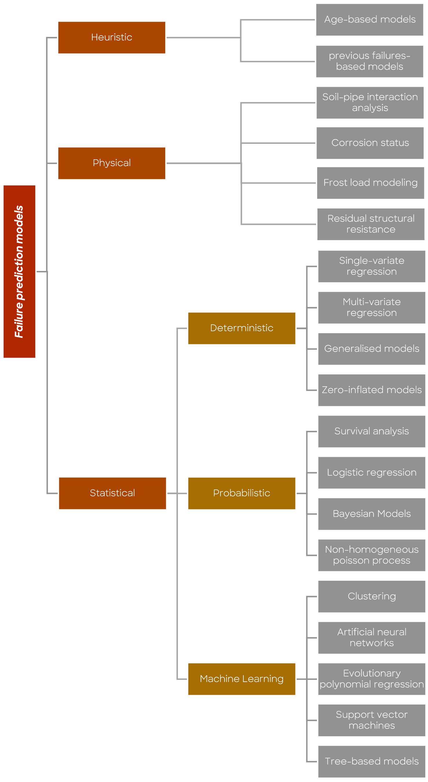
Physical models consider the underlying physical mechanisms and mechanical processes that contribute to pipe failure (Rajani and Kleiner 2001). For example, soil-pipe interaction models are used to estimate the stresses and strains on pipe walls and compare them with the remaining strength of the pipes (Rajani et al. 1996; Rajani and Makar 2000; Seica and Packer 2004; Tesfamariam et al. 2006; Farhadi and Wong 2014; Murugathasan et al. 2021). Additionally, some physical models investigate the corrosion and structural deterioration to estimate the remaining lifespan of the pipes (Zhou et al. 2012; Larin et al. 2016; Mahmoodian and Li 2015; Wasim et al. 2018; Wang et al. 2023). These models are particularly efficient when the main causes of failures are well understood. Although physical models yield accurate results, their applicability is limited to the specific pipes studied and cannot be easily generalized to other parts of the network. Consequently, these models are best suited for analyzing large-diameter pipes, which are of greater importance to asset managers due to their critical role in the infrastructure.
Statistical models utilize mathematical and statistical concepts to identify trends and relationships between independent covariates and failure parameters, such as the number of failures, failure rate, time-to-failure, and probability of failure (Kleiner and Rajani 2001). They employ pipes (assets) data and historical failure data to establish correlations between failure occurrences and contributing factors. To enhance their prediction capability, other data sources, such as pressure records, soil type data, and weather data, can be introduced to the models. The data used can be numerical (e.g., pipe length, diameter, and age) or categorical (e.g., soil type, and pipe material), each requiring appropriate handling to suit the model’s requirements (Konstantinou and Stoianov 2020). Statistical models fall into three categories: deterministic, probabilistic, and machine learning models (Nishiyama and Filion 2014; Scheidegger et al. 2015; Snider and McBean 2020; Barton et al. 2022a).
Deterministic and probabilistic models have been reviewed in detail by Scheidegger et al. (2015). These were initially developed as simple models to predict the number of failures and failure rate. Single-variate regression (Kettler and Goulter 1985), multi-variate regression (Asnaashari et al. 2009), generalized linear models (GLM) (Yamijala et al. 2009), and zero-inflated models (Konstantinou and Stoianov 2020) are examples of deterministic approaches. Time-linear (Kettler and Goulter 1985) and time-exponential (Shamir and Howard 1979) models have been used for temporal prediction of failures, wherein they are trained using past failure data to predict future failures. The use of deterministic models has been popular among water companies due to their simplistic mathematical framework and ease of interpretation. However, these models have limitations in providing comprehensive information about pipe failures, as they may not account for all relevant variables. Moreover, deterministic models are more appropriate for pipe groups. As an example, in most of the case studies, it is not easy to find a large number of pipes with multiple failures, so developing an accurate deterministic model to predict the number of failures in each pipe becomes challenging. However, deterministic models can be used to predict the number of failures in a given group of pipes.
Probabilistic models often use statistical concepts to predict the probability of failure or time-to-failure in pipes. While the deterministic models are suitable for assessing a cohort of pipes, probabilistic models are easy to apply at the asset level. Cox proportional hazard (CoxPH) models, Survival analysis (Røstum 2000; Debón et al. 2010), non-homogeneous Poisson process (NHPP) (Economou et al. 2012), Zero-inflated nonhomogeneous Poisson process (ZINHPP) (Kleiner and Rajani 2010), Weibull proportional hazard (WPH) models (Alvisi and Franchini 2010), Weibull accelerated lifetime (WAL) (Debón et al. 2010), logistic regression (LR) (Yamijala et al. 2009), and Bayesian and Naïve Bayes models (Francis et al. 2014; Tang et al. 2019) are common examples of probabilistic models. These models are flexible, can accommodate randomness, and effectively capture the complexity arising from multiple variables, making them suitable for providing valuable insight to aid in rehabilitation and replacement decisions. However, some probabilistic models, such as survival models and Bayesian models, have complex mathematical frameworks, which makes them difficult for water companies to implement as they require specialized expertise and knowledge (Barton et al. 2022a).
Machine learning (ML) models have made remarkable strides in recent years, surpassing traditional statistical models by offering enhanced predictive accuracy and expanded capabilities. Using ML algorithms, these models learn the relationships and trends by utilizing a significant portion of the data for training (train set), while the remaining data set is used to evaluate the trained model (test set). The flexibility of ML models allows them to be used for predicting number of failures, rate of failure, probability of failure, and time-to-failure. They have been effectively used for regression, classification, or as probabilistic classifiers. The previous computational challenges associated with ML models have been overcome thanks to continuous advancements in computing power. These models are capable of learning and capturing the complex correlations and trends in high-dimensional problems and large databases. ML models are particularly well-suited for application at the asset level. While they are capable of predicting the number of failures, rate of failure, time-to-failure, and probability of failure, they exhibit greater accuracy in predicting the latter. Also, tuning the hyperparameters of these models has been simplified, as it can now be carried out within the model itself for the user’s convenience.
The main ML models which have been used in the literature for pipe failure prediction are clustering (Farmani et al. 2017; Kakoudakis et al. 2017), artificial neural networks (ANN) (Tabesh et al. 2009; Kerwin et al. 2020), k-nearest neighbors (KNN) (Kutyłowska 2018), evolutionary polynomial regression (Berardi et al. 2008; Kakoudakis et al. 2018; Giraldo-González and Rodríguez 2020), support vector machines (SVM) (Kutyłowska 2019; Robles-Velasco et al. 2020), and tree-based models.
Tree-based models are a category of machine learning models which can be used for regression, classification, and even for probabilistic classification. Although they are computationally expensive, according to the literature, they have outperformed other common ML models in terms of accuracy and prediction capability. The fundamentals of these approaches are simple, and they do not require complex pre-processing, e.g., data normalization. This paper reviews various tree-based models and their application in failure prediction of water pipes. Some of the tree-based models are well known and have already been employed in this field, e.g., decision trees, random forest, gradient boosting, AdaBoost, and Catboost. Nevertheless, there are some other models which are not very known to water sector, but could be useful in overcoming the common challenges in this area such as imbalanced data, censored data, high-dimensional and complex data sets, etc.
Tree-Based Models
ML algorithms can be broadly categorized into two main types: supervised and unsupervised learning (Kim et al. 2021). Supervised ML learns from labeled data, where the algorithm is trained on previously categorized input data to make predictions for the output variables (Huang et al. 2014; Ono and Goto 2022). Supervised ML algorithms have found widespread applications in various fields. Particularly in the water sector, they have been employed for failure prediction and asset condition assessment in WDNs (Dawood et al. 2020; Barton et al. 2022b; Delnaz et al. 2023). Unsupervised ML algorithms are commonly used in clustering and anomaly detection. Clustering involves grouping related data based on shared characteristics, while anomaly detection focusses on identifying data points that deviate significantly from the rest of the data (Ono and Goto 2022). Unsupervised algorithms can learn to find patterns and relationships in data without any prior knowledge of output variable(s) (Laskov et al. 2005; Usama et al. 2019; Zoppi et al. 2021). Unsupervised learning has been mostly used to improve water pipe failure predictions (Kakoudakis et al. 2017).
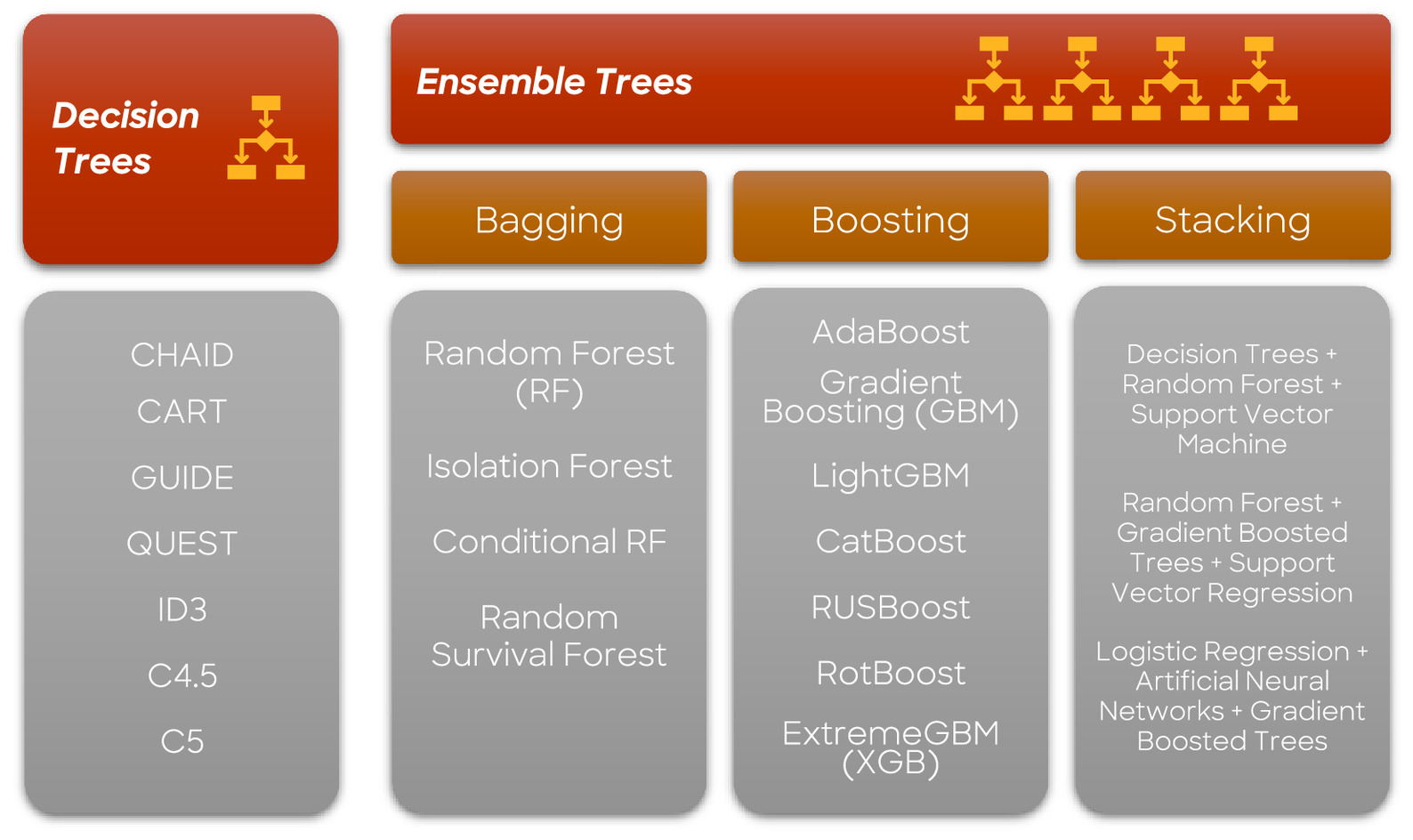
Tree-based machine learning models, a subset of supervised learning algorithms, utilize decision trees to make predictions. Their popularity has grown significantly in recent years due to their exceptional accuracy, robustness, and interpretability (Kumar 2019). These models can be categorized into two main groups: decision tree algorithms, and ensemble learning methods, which include bagging, boosting, and stacking strategies (Fig. 2) (Jafarzadeh et al. 2021). Decision tree algorithms utilize the feature values of the input data to partition the data space into smaller regions recursively (Xiaohe et al. 2014; Coadou 2022). Conversely, ensemble tree algorithms improve model accuracy and robustness by combining multiple decision trees (Mishina et al. 2015). During the model creation process, some trees (learners) may be weak, and that is where boosting strategies combine multiple weak learners to create a stronger learner (Nishio et al. 2018; Coadou 2022). The following section reviews these tree-based ML algorithms, along with relevant examples.
Decision Trees
A decision tree (DT) is a supervised machine learning algorithm that handles classification and regression problems. Its name comes from its treelike structure. When predicting the class of a data set, the DT algorithm starts at the root node, which represents the entire population, and compares the feature values of the root node with the record features. Based on this comparison, the algorithm follows the corresponding branch to the next node. The process continues until it reaches the final node (leaf) in the tree.
Fig. 3 demonstrates a simple instance where WDN data was utilized to predict pipe failure. The example employs three features: pipe type (main or service), length, and age. The data set’s pipe type feature is used to create two sub-nodes from the root node based on a yes-or-no condition. The age feature is then utilized for further splitting, with ages above 50 years serving as branch nodes, and failed as the resulting leaf node. Another branch is created using the length feature. After three splits using these features, failed and not-failed become leaf nodes, and no further splitting occurs.
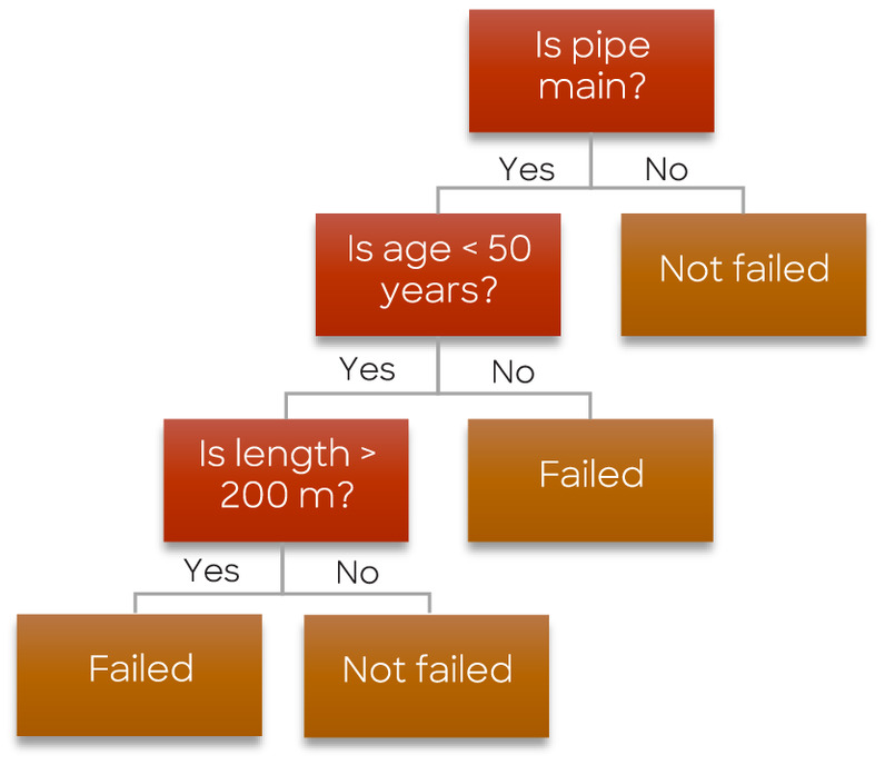
The careful selection of the root node and sub-nodes is crucial in implementing the DT algorithm, significantly influencing its performance. To achieve this, attribute selection measures (ASMs) are employed to choose the most relevant attributes for classification. Different ASMs have been developed for this purpose, including entropy, information gain, and the Gini index (Liu et al. 2004; Nnebedum 2012; Katterbauer et al. 2022; Li and Yin 2023).
The following section covers a brief explanation and mathematical formulation of some of the main ASMs. Entropy is a fundamental measure that quantifies uncertainty or randomness within a given data set. In the context of DT, entropy is utilized to evaluate the impurity of a specific node or a subset of data. The entropy value assigned to the root node reflects the overall impurity of the entire data set, while within subsequent sub-nodes it characterizes the impurity of the corresponding subset of data governed by the respective decision. Mathematically, entropy is expressed as:where is the entropy of the set (); and is the portion of the number of elements in () that belongs to the th class (Li et al. 2011).
(1)
Information gain (IG) is a measure utilized to decrease uncertainty in a manner similar to entropy. It determines the most suitable feature for splitting the root node into sub-nodes, thereby minimizing impurity in the resulting subsets. The feature with the highest IG value is selected as the preferred splitting criterion. The calculation of IG is represented as follows:in which, is the information gain of splitting set () and feature (); is the proportion of elements in subset relative to the number of elements in () (Batra and Agrawal 2017).
(2)
The Gini impurity index, like entropy, serves as an alternative measure of impurity or randomness in DTs. It quantifies the likelihood of misclassifying a randomly selected element from a set, assuming random labeling according to the label distribution within the subset. By considering the proportions of different classes or labels within a data subset, the Gini index captures the extent of impurity or randomness in that subset (Tangirala 2020; Smith et al. 2022). The Gini index is calculated aswhere has been defined in Eq. (1).
(3)
DT models have evolved over time and have been utilized in various domains. In this review, we explore some of the renowned DT models that have emerged throughout the history of their development. Fig. 4 presents a timeline of the evolution of tree-based models.
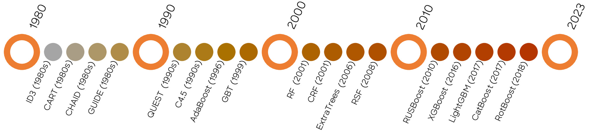
The chi-squared automatic interaction detector (CHAID) model is one of the primary tree-based classification algorithms. This algorithm partitions data based on the chi-square test and stops the partitioning process when a threshold of statistical significance is reached (Kass 1980; Jagtiani and Henderson 2010; Tamaoka et al. 2010).
Interpreting the CHAID model is intricate due to its use of multiway splits, specifically designed for categorical data analysis. Notably, the computational demands of the CHAID algorithm arise from the calculation of chi-square statistics for each potential split. In response to the need for managing both classification and regression tasks involving categorical and numerical data, and to address the challenges associated with CHAID, classification and regression trees (CART) was introduced (Breiman 1984). This algorithm utilizes the Gini index as a measure of impurity to establish splitting criteria. CART has proven to be highly successful and widely employed in diverse fields, particularly in failure prediction modeling. It is noteworthy that CART can be regarded as the progenitor of other tree-based algorithms (Tamura et al. 2019; Brédart et al. 2021; Wieczorek et al. 2021; Fiosina et al. 2023). Although CART was a successful algorithm, it had certain limitations, such as sensitivity to small changes in data and susceptibility to overfitting. To address these shortcomings, generalized, unbiased, interaction detection, and estimation (GUIDE) was developed (Loh and Shih 1997). Based on recursive partitioning, this method is considered more robust and proficient in handling complex relationships between variables. It also provides unbiased variable selection, enhancing its reliability and accuracy in modeling tasks (Kang et al. 2010; Lee 2021). CART was further developed by introducing a non-parametric method called quick unbiased efficient statistical tree (QUEST) (Breiman 1984). This algorithm is highly recognized for its ability to handle large data sets and its unbiased nature, as it does not make any assumptions about the underlying distribution of the data (Lee and Lee 2015; Song et al. 2020).
Moreover, to accommodate both categorical and continuous features, an array of approaches were proposed for partitioning the data into subsets based on different feature categories and employing binary splits for continuous variables. This concept underwent further refinements, leading to the development of the Quinlan decision tree (QDT) algorithm, also known as the iterative dichotomizer 3 (ID3) (Quinlan 1990). Other algorithms, such as C4.5 and C5.0, were later developed to overcome shortcomings, e.g., the tendency to overfit (Quinlan 1992; Nanda et al. 2011).
Ensemble Learning
Ensemble learning is an ML methodology that aims to improve prediction accuracy and robustness by combining the predictions of multiple models. It addresses the issues of errors and overfitting that may arise in individual models by harnessing the collective power of multiple models. Combined models can be of the same type or different types. Over time, various techniques have been developed for implementing ensemble learning, which have evolved in their capabilities and applications across different fields (Webb and Zheng 2004; Yang et al. 2010).
Extremely randomized trees (ExtraTrees) is one of the primary ensemble methods that builds multiple DTs and combines their outputs to make a final prediction. The trees in ExtraTrees are constructed using random splits of the input features and random thresholds for each split, which makes it less prone to overfitting than traditional DTs (Geurts et al. 2006).
Various approaches have been introduced for ensemble learning, and the main success point of these methods is diversity. Here diversity refers to generating multiple subsets from the original data set to train different predictors such that the outputs of the predictors are diverse (Ganaie et al. 2021). Ensemble approaches are broadly categorized as bagging, boosting, and stacking.
Bootstrap Aggregating (Bagging)
Bootstrap aggregating, also referred to as bagging, is an ensemble learning approach employed to create numerous subsets of the original data set through random sampling and training separate models on each subset (Fig. 5). Bagging proves particularly beneficial when working with limited data sets that are prone to overfitting. This approach is not limited solely to DT models, as it can be applied to various models, such as ANN and SVM (Mehmood et al. 2019; Muhammad et al. 2020; Modabbernia et al. 2022).
Random Forest (RF) is an ensemble ML approach that improves model accuracy and robustness by employing multiple base DTs. This approach utilizes a bagging strategy to enhance predictive capability by randomly selecting a subset of features and aims to mitigate overfitting by decorrelating each tree (Breiman 2001; Kulkarni and Sinha 2012; Shahhosseini and Hu 2020; Ogunleye 2022). Isolation forest is an unsupervised algorithm developed by using the bagging strategy. It is renowned for its ability to detect anomalies without using traditional measures such as density, which refers to the concentration of data points in a data set, and distance, which represents the spatial separation between data points. Instead, the isolation forest algorithm utilizes alternative approaches based on DT to identify anomalies. These distinctive features make isolation forest stand out in anomaly detection, as it does not rely on density or distance measures commonly employed by other algorithms (Hastuti et al. 2020; Suriyanarayanan and Kunasekaran 2020). Conditional random forest (CRF) was introduced as an algorithm that combines RF and a graphical model called conditional random fields, which is utilized to establish connections between input and output variables by employing a collection of potential functions (Kong et al. 2021). The idea of CRF is based on modeling the dependencies between the output variables using a graph structure. The graph structure in the CRF model allows it to effectively capture and exploit correlations and interactions among the output variables. This is achieved by organizing and modeling the connections between these variables using a graph, where the output variables are represented as nodes, and the dependencies between them are indicated by edges (Kaczałek and Borkowski 2016; Kumbhakarna et al. 2020). The random survival forest algorithm is another method that constructs an ensemble of DTs to predict survival probability, which entails predicting the likelihood of an event occurring within a specified time frame (Ishwaran et al. 2008).
Boosting
Boosting is a sequential strategy that involves building models in a cascading manner, with each subsequent model aiming to correct the errors made by its predecessor. In this strategy, the succeeding models depend on the performance and insights gained from the previous models. An initial subset is generated from the original data set with equal weights assigned to each data point. A base model is created using the initial subset, and subsequently, predictions are made on the entire data set using this model. The errors are then calculated by comparing the actual and predicted values. To take the errors into account and reduce them, incorrect data points are assigned higher weights, and a new model is created. Iteratively, several models are created, each correcting the errors of the previous model. The final model, regarded as a strong model, is derived by calculating a weighted average of all the previously created weak models (Fig. 6). These weak models, while not performing well individually on the entire data set, exhibit effectiveness in specific areas of the data. Consequently, each model contributes to enhancing the overall performance of the ensemble, resulting in a boosted performance (Schapire 1999; Mayr et al. 2014).
Adaptive boosting (AdaBoost) and gradient boosting trees (GBT) are two well-known examples of boosting strategies that have been widely employed in various domains. AdaBoost utilizes a collection of small decision trees called stumps, each with a maximum depth of one. This implies that the tree comprises a sole root node and two leaf nodes, permitting only a single decision split to occur. The main objective of AdaBoost is to minimize misclassifications by iteratively improving the current model by including a properly weighted predictor (Freund and Schapire 1996). GBT follows a similar boosting strategy to AdaBoost, aiming to minimize the loss function (a mathematical function to measure the error between prediction and actual values) by fitting subsequent models to the negative gradient of the loss. However, there is a subtle difference in their implementation. While AdaBoost commonly uses decision stumps as weak models, GBT is more flexible and can employ various weak models, including decision trees with larger depths (Friedman 2002). This allows GBT to capture more complex relationships in the data and potentially achieve higher accuracy compared to AdaBoost (Luo and Spindler 2016; Saez et al. 2016; Kwon et al. 2017; Toghani and Allen 2020; Anjum et al. 2022).
Light gradient boosting machine (LightGBM) has gained popularity for large-scale machine learning tasks. It incorporates a technique called gradient-based one-side sampling (GOSS) to reduce the number of samples used during training. This approach significantly accelerates the training process while maintaining predictability (Ke et al. 2017).
The categorical boosting algorithm (CatBoost) is specifically designed to handle categorical variables without needing one-hot encoding (Hancock and Khoshgoftaar 2020) or extensive preprocessing steps. This saves time and mitigates the risk of overfitting, particularly when dealing with categorical features with high cardinality.
Extreme gradient boosting (XGB) is another well-known and widely used algorithm. It operates by iteratively adding DTs, subsequently building a collection of weak predictive models, known as weak learners, which are then combined to form a robust predictive model. XGB has gained widespread recognition for its outstanding performance in various machine learning competitions hosted on platforms like Kaggle, known for its data science competitions (Hasani and Nasiri 2021), and its ability to handle missing data. XGB was used for both regression and classification tasks, and it performed well at both (Jafarzadeh et al. 2021; Tervonen et al. 2021). This method has also the ability to automatically learn the optimal imputation of missing values based on the available data (Jafarzadeh et al. 2021; Zhongyuan et al. 2022; Siregar et al. 2022).
Random undersampling boosting (RUSBoost) is also an ensemble learning algorithm, utilizing boosting strategy developed to address class imbalance problems in binary classification tasks (Seiffert et al. 2010). It is worth noting that boosting algorithms, such as RotBoost (Zhang and Zhang 2008), which combines rotation forest and AdaBoost, showcases the effectiveness of the boosting strategy when utilized in conjunction with other algorithms, demonstrating impressive accuracy.
Stacking
Stacking is an ensemble learning strategy that utilizes predictions from multiple models to construct a new model. It is also known as a meta-learning method, as it integrates the outputs of base models and serves as a valuable approach to reducing bias (Mallick et al. 2022). In this strategy (Fig. 7), the training data set is divided into subsets. A base model, such as a DT, is trained on subsets of the data, and then used to predict the th subset. These steps are repeated for each base model, resulting in a set of predictions for both the training and testing data sets. The predictions from the training data set are then employed as features to build a new model, which is subsequently used to make final predictions on the testing data set (Ganaie et al. 2021).
Several studies have used tree-based models as one or two of the base models in the ensemble. Stacking strategy, which incorporates tree-based models like DT, RF, and GBT, has found application in various domains such as estimating the amount of time, resources, and effort required for developing software, analyzing COVID-19 vaccine sentiments, predicting air quality index and using a blending approach in stacking for detecting botnet attacks in computer network traffic (Ag and Varadarajan 2021; Jain and Kashyap 2022; Afrifa et al. 2023; Gupta et al. 2023). The stacking strategy was also employed in evaluating the performance of water mains to optimize pipeline rehabilitation and to enhance the prediction of pipe conditions (Shi et al. 2017).
Evaluation Metrics
Various metrics have been proposed for the evaluation of ML prediction models. Selecting the right metric depends on the type of problem and output of the models (Vaags 2021). Each evaluation metric should be understood carefully before they are employed. Using unrelated metrics could be misleading in assessing the performance of the models, and lead to either overestimation or underestimation of their prediction capabilities (Jin et al. 2019; Rahim et al. 2021). Furthermore, traditional evaluation metrics are not able to comprehensively assess the capability of failure prediction models for pipes. This limitation results from their tendency to consider equal value for each member of the data set, i.e., pipes. As an example, correctly predicting the failure in a pipe with large diameter and length should not be equated with forecasting the failure in a short, small diameter pipe. Hence, reduction in failures versus cost of pipe replacement, and saved capacity of WDN versus replacement costs are some options to evaluate the performance of a prediction model more practically (Beig Zali et al. 2024). Another illustrative example is the work of Robles-Velasco et al. (2020) where they considered the percentage of failures avoidance by replacing 5% of high-risk pipes, i.e., 5% of the pipes with the highest likelihood of failure. Such measures not only make more sense to the engineers, but also provide decision makers with a clear understanding of the effectiveness of each approach. Some of the most commonly used metrics are introduced in Appendix I. Based on their purpose, evaluation metrics are categorized into three distinct groups: (1) regression, (2) classification, and (3) ranking. In each category, the metrics are defined, and their application is discussed. This section can serve as a guide for researchers to select the best metrics to assess their prediction models.
Application of Tree-Based Models in Sewer Pipes Assessment
Some of the most well-known tree-based approaches have been employed in evaluating the pipes’ condition and predicting the failures in sewer and wastewater systems. Here, wastewater systems are those only carry sewage, while sewer systems collect both sewage and stormwater. In most cases, tree-based models have been compared with statistical and ML approaches, to identify the model that exhibits the highest level of performance. Appendix II presents a summary of the previous research utilizing the tree-based models in this particular field.
Condition Assessment Using CCTV Footage
Since 2014, several studies have been conducted to forecast the state of sewers using network data. In the majority of cases, the necessary information for assessing the pipes has been collected through CCTV inspections of the pipes. Tree-based classifiers, specifically the RF method, were utilized to categorize the pipes into condition groups, often consisting of five groups. Subsequently, all the pipes were classified into two primary categories: those in poor condition and those in good condition. Harvey and McBean (2014) used RF to label the sewers in the City of Guelph, Ontario, Canada. After inspecting 123 km of the gravity pipes by CCTV, all pipes were assigned an internal condition grade (ICG) of 1–5. Pipes’ length, diameter, age, material, slope, road coverage, land use, and census tract, to name a few, were used to train a model to classify all pipes into two categories of pipes with good structure (ICG of 1–3), and those with poor structure (ICG of 4–5). The database suffered from a class imbalance of 11%, i.e., only 11% of the data belonged to poor structure class. However, they did not mention their approach for dealing with class imbalance issue. While the model trained with the aforementioned data achieved an AUC of 0.81, introducing the neighboring pipes conditions to the model increased its AUC to 0.85.
Vitorino et al. (2014) applied the same approach to predict the membership of the sewers to pre-defined condition classes (1–5). While the sewers had been inspected by CCTV, they employed pipes’ length, diameter, age, material, zone, condition at the previous inspection, and so on to train an RF model for predicting the pipe’s current condition. Although they did not present the variable importance matrix, it seems that the condition class at previous inspection feature had the strongest influence on the predictive capability of the model, particularly when the pipes were inspected on a regular basis. Wu et al. (2013) employed AdaBoost, RF, rotation forest, and RotBoost, along with SVM and neural networks, as ensemble classifiers for pipe defect classification. Sewer scanner and evaluation technology (SSET) was used, as a visual inspection technique for sewer pipelines, to take footage from the internal space of pipes. Using the outputs of image processing as input variables to classifiers, RotBoost outperformed the other classifiers in accuracy.
Rokstad and Ugarelli (2015) employed RF along with GompitZ [which is a sewer deterioration model (Sægrov and Schilling 2002) based on a nonhomogeneous Markov Chain model], for the classification of the individual sewer pipes (Le Gat 2008). In their research, diameter, wastewater type, construction era, road traffic, soil type, and presence of tree roots in CCTV images were used for predicting the condition class of the pipes in the sewer system of Oslo, Norway. The developed models were not highly predictive due to several factors, including the lack of explicit consideration of specific failure modes, inadequate inclusion of appropriate covariates, and potential insufficiency of the model assumptions.
Myrans et al. (2018) used the CCTV frames from sewer networks of Wessex Water, UK, to detect the failures in sewer pipes. A data set of 1,500 frames was manually labeled based on the manual of sewer condition classification (WRc plc 2013). The labeled data set was used as the training data for RF and SVM classifiers. Image feature descriptors, such as GIST, were used as model training inputs. While RF and SVM yielded AUC of 0.83 and 0.77, respectively, their results were combined to enhance the results considering three approaches: take the most likely prediction from the pair of classifiers, use both classifiers’ outputs as inputs, and use stacking. Among these approaches, the weighted stacking method led to a slightly larger AUC (). Myrans et al. (2019) used the same input data (CCTV footage) to predict the type of detected failure in sewers. 13 failure types, including joints, deposits, cracks, surface, roots, etc. were defined and assigned to each failure. The employed techniques achieved accuracies over 60%, indicating their merit in assisting the inspectors in determining the fault types.
The ability of tree-based models to consider various input variables allows them to outperform other ML algorithms, when it comes to complex classification problems, such as learning from CCTV footage and predicting the condition of unseen pipes. Taking the more relevant variables and stacking the weaker algorithms leads to higher prediction accuracy. Combining several classifiers makes it possible even to determine the type of failure in sewers with reasonable accuracy (Myrans et al. 2019). Malek Mohammadi et al. (2020) employed GBT algorithms to predict the sewers condition through CCTV footage. Although they used pH, sulphate content, water table, soil hydraulic group, and soil corrosivity, the main predictive variables of the model were age, length, and diameter.
Pipe Condition Assessment Using Static Data
Static data are the features of the pipes or network which do not change (e.g., pipe material and length), or change very gradually (e.g., pipe diameter and thickness), in a way that they can be considered constant in a case study. Soil type and installation date are other examples of static data in a water or sewer network. Syachrani et al. (2012) employed DT in predicting the real age of sewer pipelines, which is defined as an adjusted age given the pipes’ location and operation conditions. They calculated this factor as the mean age of the pipes which fall in a particular cluster (leaf). MSE can be used as the performance indicator for the prediction model; the lower the MSE, the higher the predictive capability. Conversely, lower MSE values in a given cluster represent the lower heterogeneity. They applied the DT along with a simple regression and ANN model, in a case study of 95 km pressurized and 3,219 km gravity sewer pipes in Kansas, US. All models used length, diameter, material, slope, pipe condition value (between 1 and 5), and problem type (e.g., debris, sludge, roots, etc.) as the input variables. They focused on vitrified clay pipes (VCP) and PVC pipes. The results showed that DT outperformed the other methods, in terms of ASE, MAE, and RMSE.
Santos et al. (2017) used CART, RF, Robust Tree and Robust Forest, NHPP, ZINHPP, and WAL models and the linear extended Yule process (Le Gat 2013) to predict failure in individual pipes in a sewer network in the US. Pipes’ diameter, length, age, material, and slope were considered as input variables. To assess the prediction capability of the models, they presented the percentage of avoided failures as a function of the rehabilitated length (percentage). Specifically, the analysis indicates that a small percentage of the pipes’ length being rehabilitated can potentially result in avoiding a significant number of failures. This is a more practical measure of the predictive capability, in comparison with precision, recall, accuracy, F1-score, or AUC. This is because in a water/sewer network, each pipe has its own length, diameter, cost of rehabilitation, and consequence of failure, which should be considered rather than the number of replaced pipes. The selected model, robust forest, was able to capture 13% of failures by rehabilitating only 1% of the pipes’ length.
Tavakoli et al. (2020) utilized an RF classifier to predict the pipe condition in sewers. Diameter, length, age, material, slope, depth of cover, age at the time of inspection, upstream and downstream elevations, etc. of a sewer network in Los Angeles, US, were employed as the input variables. Their best-selected model resulted in an AUC of 0.80. Van Nguyen and Seidu (2022) selected a wide range of regression models, including CART, RF, extra trees regression (ETR), AdaBoost, GBT, histogram-based GBT along with Gaussian process regression (GPR), KNN, SVR, and MLPNN to predict the sewer’s condition. Among all these models, ETR, GPR, and RF exhibited higher accuracies, respectively.
In order to split the data set to a train set and a test set, two methods can be utilized; (1) temporal split, i.e., training the model with entire assets data from a part of historical failures data, and then evaluating the model against the failures that occurred in the remaining part of failures, and (2) random split, i.e., randomly dividing the whole asset into two parts, one for training and the other for testing the model. Temporal split showed better results, in comparison with random split. It also provides the ability to predict future failures (Santos et al. 2017).
Application of Tree-Based Models in Water Pipes Assessment
Pipe Condition Assessment
Early failure prediction models for water pipes were developed to assess and predict their condition. Jilong (2014) utilized the C4.5 algorithm for the classification of water pipes into three conditions/categories: unserviceable, near-perfect condition, and serious deterioration. In addition to the common variables (diameter, age, material, pressure), distance to pump, distance to tank, and pipe load were considered as explanatory covariates for pipe condition prediction.
Shi et al. (2018) employed and RF model, besides multiple linear regression, SVM, and ANN, for pipe condition rating based on remaining pipe thickness in CI pipes. As input variables, they used pipes’ wall thickness; soil type; soil resistivity; soil pH; soil sulfite content; soil moisture; and soil corrosivity, to develop a model with more accuracy than previous ones. Based on the results, RF had the least RMSE, while SVM reached the highest . Furthermore, stacking all four algorithms led to an assessment model with better performance than each.
Mazumder et al. (2021) employed tree-based algorithms DT, RF, AdaBoost, XGB, LightBoost, and CatBoost along with KNN and Naïve Bayes for categorizing steel oil and gas pipes, based on their failure pressure, into four classes of failure probability (low, moderate, high, and severe). The models were trained on a data set of 92 experiments from the literature to predict the pipes’ conditions. CatBoost, XGB, and LightBoost presented the highest accuracy () than the others. While the study focused on oil and gas pipelines, its relevance to WDNs lies in the similarity of failure patterns, making it a noteworthy addition to this review. Assad and Bouferguene (2021) used tree-based algorithms like DT, RF, XGB and AdaBoost along with a range of other ML methods, e.g., GLM, KNN, Deep Learning, and SVM to predict the pipe condition score (1–10) in Waterloo, Canada. Among the utilized approaches, XGB and RF proved highest performance in predicting the actual condition of the pipes in test set. Pipe material, number of previous bursts and age were shown to be the most important attributes.
Estimating Time-to-Failure
Snider and McBean (2018) used RF, XGB, and ANN to predict the time-to-failure for 339 km of ductile iron (DI) pipes in a North American water utility. Cement mortar lining year, cathodic protection year, pressure, break density, number of previously recorded failures, and break age for all previously recorded failures were used to train the models. Tuning all three models, RF and XGB presented considerably better RMSE and values than the ANN. Snider and McBean (2019) compared XGB (as a representative of ML algorithms) with the WPH model (as a survival analysis model) in predicting the time-to-failure in a case study of a WDN in Canada with failure records between 1960 and 2016. They concluded that the ML model works well in short-term predictions; however, when it comes to long-term break patterns, the model does not include the censored events, which compromises its ability to predict the pipe-break events. In addition to WHP and XGB, Snider and McBean (2020) developed two more heuristic models based on age and previous breaks in each pipe. They split the failure record and pipe data sets into subsets to study the effect of data limitation on predictive capability. As expected, data shortage, either temporal or record-wise, downgraded the predictivity of the models. However, when it came to training the models with more than 5 years of failure data and more than 2,000 pipes in the training data set, XGB outperformed all the other approaches. Additionally, among the algorithms tested, XGB demonstrated the highest robustness against missing data. Snider and McBean (2021) utilized random survival forest (RSF), a combination of RF and Weibull survival models, for predicting the time-to-failure in the same case study. The RSF model worked significantly better than each of the constituent models.
Almheiri et al. (2020) employed ensembled decision trees (EDT) along with ANN and regression models (Tibshirani 1996) to predict the time-to-failure in gray CI, DI with/without lining, PVC, and hyprescon/concrete water pipes. Although regression presented the least RMSE and MAE, and the highest R among the three models, the authors recommended the EDT model for prediction due to its simplicity, computational efficiency, and ability to deal with both categorical and continuous variables. Yang et al. (2020) used simple DT to predict the survival of the pipes in China. They clustered all features into groups, in order to make the DT training easier. However, the accuracy of their model did not exceed 8%. They found that the time passed from previous failure and month of the year have the major impacts on the probability of failure in each pipe.
Training a model to predict time-to-failure at the pipe level requires long-term failure data, i.e., in short-term (censored) data tree-based models suffer from limited accuracy. Combining tree-based models with statistical models, e.g., survival models, covers their weaknesses and results in models with higher concordance.
Predicting Individual Pipes Failures
Predicting pipe failure within a specific time frame has consistently remained an intriguing area of interest for researchers. Winkler et al. (2018) studied 851 km of a WDN in Austria, with failure data since 1983. They employed DT, RF, AdaBoost, and RUSBoost to classify the individual pipes into either failed or non-failed groups. This paper stands out as a notable contribution that compares the effectiveness of tree-based models for classification purposes. Among the four models, RF and AdaBoost demonstrated the lowest false negative rate (FNR), while RUSBoost exhibited the least false positive rate (FPR). Although all methods showed similar Area Under Curve (AUC) values, RUSBoost achieved the highest AUC of 0.93, demonstrating its exceptional predictive capabilities. Leveraging an extensive historical record of pipe failures, the study harnessed common pipe features such as diameter, length, age, material, pressure, and pipe type, to achieve such high prediction performance.
Chen and Guikema (2020) utilized density-based scanning (DBSCAN) (Sander et al. 1998) spatial clustering to identify areas with high failure rates. These data were fed to ML models such as GLM, generalized additive models (GAM), regression trees, RF and GBT, to enhance the prediction accuracy. Among these models, RF yielded significantly better predictions, based on break capture versus pipe replacement length. In addition to the common features, they used average pressure, average flow, proximity to major roads, soil corrosivity and frost potential, land use, and climatological data, as explanatory features for failure prediction.
Giraldo-González and Rodríguez (2020) investigated a case study of a WDN in Bogotá, Columbia. They utilized four different models, GBT, Bayesian, SVM, and ANN, for a classification task involving two types of pipe materials: PVC and AC. The objective was to determine whether the pipes would fail or not. Based on the analysis of the predicted outcomes, the study concluded that GBT and Bayesian outperformed the other models in terms of accurately predicting failures and reducing false predictions. Konstantinou and Stoianov (2020) used RF for predicting the annual number of failures per pipe segment and for the whole WDN, along with time linear models, time exponential model, Poisson GLM, and naïve Bayes algorithm. In all cases, RF delivered the most accurate predictions, both in training and testing.
Fan et al. (2021) used LightGBM besides ANN, LR, KNN, and SVM classification to predict pipe failure in a specific year. In addition to diameter, length, age, material, number of previous breaks, and time-to-previous break, they utilized soil type, topographical data, census data (population, health insurance, and poverty), and climate data (hot/cold days). The correlation matrix of the covariates indicated low impact of census data, and high impact of age and climate data on the target. LightGBM model showed the highest area under the ROC and PRC curves among utilized models, which could be because of its ability to handle categorical variables without one-hot-encoding. Liu et al. (2022) employed RF and LR models for classifying the pipes in 1,100 km water pipes in China. Due to the class imbalance nature of the data, different treatment methods were implemented, such as the synthetic minority oversampling technique (SMOTE) (Chawla et al. 2002), oversampling, and undersampling. In all cases, RF yielded higher accuracy, recall, and AUC than LR. Nevertheless, the authors did not present the precision of the models, which is a key indicator of catching true positives among all positives. In data with imbalanced nature, increasing the precision is still a great challenge, even after applying balancing techniques.
Evaluating Failure Rate
The failure rate is often defined as the number of failures per unit length of pipes per unit of time, for which is a standard unit. Therefore, the failure rate could be predicted for a group of pipes, usually pipes in an area (e.g., a DMA), or pipes with similar properties (e.g., material, or age). This factor gives an insight to the operators about the vulnerability of a part of WDN. Shirzad and Safari (2019) compared the performance of multivariate adaptive regression splines (MARS) with RF in predicting the failure rate. Both regression models were trained with pipes’ diameter, length, age, installation depth, and average hydraulic pressure, for two case study WDNs of 139 km and 579 km. In the smaller case study, RF achieved to RMSE, MAE and of 0.31, 0.05, and 0.97, respectively, which indicates that it significantly outperformed the MARS, with 0.71, 0.36, and 0.84, respectively. In the larger WDN, both regressors worked perfectly, with RF performing slightly better. Wols et al. (2018) employed a gradient boosting regressor for predicting the failure rate in 97,000 km of water pipes in the Netherlands, which is the largest data set in terms of pipe length, in this review. They used diameter, age, material, soil type, and regional weather data, e.g., mean daily air temperature, maximum daily wind gust at ground level, daily precipitation amount, and potential evapotranspiration (i.e., rain deficit). This is one of the few studies that have used climate and soil settlement data as factors for predicting the failure rate.
Aslani et al. (2021) developed RF, boosted regression trees (BRT), MARS, and ANN, to predict the failure rate in a WDN in Florida, US. BRT exhibited the best performance in terms of RMSE and MAE in the test sets. They also used ICOMP, AIC, and CAIC metrics for ranking the performance of the models.
Although most of the models have incorporated environmental data, e.g., soil data, weather data, pipe bedding conditions, etc., into failure prediction models, only a few have shown a high correlation between environmental characteristics and failures. Nonetheless, when there was such a relationship, tree-based models often outperformed other approaches.
Probability/Likelihood of Failure
Konstantinou and Stoianov (2020) used RF and XGB besides ANN, logistic GLM, and linear discriminant (Tsitsifli et al. 2006) analysis to predict the probability of failure. The tree-based models achieved an AUC of almost 1, while the best AUC for the other models was not higher than 0.84. In addition to common pipe properties, maximum daily pressure and temperature, daily pressure, and temperature ranges, corrosivity, fracture potential, etc. were employed as explanatory features.
Vaags (2021) used XGB survival embedding (XGBSE) (Loft Data Science Team 2021), random survival forest (RSF) (Weeraddana et al. 2021), polynomial regression, CoxPH, WPH, and neural multitask logistic regression for predicting the likelihood of failure (LoF) in four utilities in Canada. They considered diameter, length, age, material, soil type and resistivity, number of previous breaks, pressure, rainfall, temperature, flow, pump station proximity, water conductivity, etc., to enhance the accuracy of predictions. In all cases, XGBSE and RSF captured a larger number of failures compared to the other models. The capability of the models for ranking the pipes was evaluated with C-index, in which XGBSE and RSF reached the highest values. Dimas et al. (2022) compared the efficiency of a DT regression model with a KNN regression model, in three case study WDNs. Although they used simple covariates, such as diameter, length, material, and the main flagging (1 for main pipes, 0 for secondary/tertiary pipes), they achieved high accuracy, particularly for DT. They did not mention the length of available failure data for any of the case studies.
Barton et al. (2022b) applied XGB to a UK WDN of 38,400 km pipes to estimate the LoF and rank the pipes. They used MCC and FNR index to select the best threshold for deciding whether a pipe fails or not. To enhance AUC values, they utilized various sets of data, e.g., number of previous breaks, length, diameter, age, material, water source, air frost, weekly soil moisture deficit and temperature, and type, corrosivity, clay content, and shrink-swelling potential of soil. Their proposed model achieved an AUC of 0.89, one of the highest values in the literature.
Increasing the depth of trees in tree-based models enhances predictivity in the training phase. However, this may lead to overfitting when applied to the test set. Deepening the trees in tree-based models tends to capture more specific details from the training data, but this may not generalize effectively to unseen or test data. Furthermore, deep trees have the ability to memorize noise and outliers during the training phase, potentially leading to poor performance when dealing with new data. Also, their sensitivity to even minor variations in the training set can cause significant changes in the trained structure of the tree, resulting in different splits and branches for data sets with similar characteristics, ultimately compromising the model’s robustness. To mitigate this issue, hyperparameter tuning becomes necessary to optimize the model’s input parameters (not variables). This allows to achieve the best prediction performance and prevents the model from overfitting.
Discussion and Conclusion
Tree-based models, including decision trees (DTs), bagging, boosting, and stacking, are widely used in machine learning. Beginning with the most straightforward approach, decision trees offer an easily interpretable visualization of the decision-making process. They can capture nonlinear relationships between features and target variables, and handle both categorical and numerical data. However, decision trees have some inherent limitations, which have paved the way for the development of improved models. One such drawback is their tendency to overfit the training data, resulting in poor performance on unseen test data. Additionally, decision trees are sensitive to small changes in the training data, and their high variance can lead to a lack of robustness in the model.
To address the problem of overfitting, researchers have introduced a concept of combining multiple DT models, e.g., bagging, boosting, and stacking. This approach improves the development of the models by averaging their predictions and effectively addressing overfitting concerns. For instance, in the case of the bagging strategy, using multiple models trained on different data subsets helps reduce overfitting by decreasing the overall variance of the model. Similarly, in boosting, the emphasis on error correction works to decrease bias and variance, thereby resulting in reduced overfitting. Furthermore, stacking contributes to the reduction of overfitting by harnessing the strengths of different models and ensuring that the final prediction is founded on a more comprehensive and robust understanding of the data. Moreover, this approach leads to the creation of a more stable model that is less sensitive to variations in the data set, resulting in improved robustness. Additionally, this technique enables the handling of data sets with a large number of features without requiring feature selection techniques. However, it is essential to note that the bagging strategy comes with inevitable trade-offs. These include reduced interpretability compared to a single DT model, increased computational complexity due to the generation of multiple trees, and the necessity of more memory resources. Nonetheless, researchers would be willing to accept these compromises in order to leverage the benefits of bagging within tree-based models.
The issue of bias toward the majority class in DT and bagging models, particularly in imbalanced data sets, is effectively addressed by the boosting strategy, which focuses on misclassified samples and significantly enhances predictive capability. However, these models also have some limitations. They can be sensitive to outliers in the data and typically require a longer training time compared to other methods. Moreover, an increased number of boosting iterations potentially leads to overfitting, highlighting the importance of careful hyperparameter tuning, which can be time-consuming and demanding in these models.
As researchers strive to enhance the predictive performance of their proposed models, the development of the stacking strategy becomes a natural focus. This strategy combines the predictions of multiple models, leveraging their individual strengths and significantly improving the overall prediction capability. Stacking allows for the utilization of diverse model types, including tree-based models, thereby enabling flexibility in capturing complex feature relationships. However, it is valuable to acknowledge the drawbacks associated with this strategy. Implementing and tuning stacking models require additional effort compared to individual models. Furthermore, constructing a meta-model within this strategy might be computationally expensive. Additionally, in a world where explainable computational intelligence is highly valued, it is worth noting that stacking models are challenging to interpret.
In summary, the decision on which model to use for decision-making depends on the specific needs and priorities within a given context. For instance, DT excels at providing clear explanations and interpretations but can be sensitive to data. Alternatively, RF, which utilizes multiple DTs, offers robustness and predictive accuracy, but presents challenges in terms of interpretation and can be computationally intensive when large number of trees need to be trained.
Statistical analysis of the research conducted in this domain indicates an increase in employing of tree-based models for failure prediction in water and sewer systems. Fig. 8(a) shows the increasing trend since 2018, and the higher number of studies on water systems in comparison with sewer systems. Usage of the three most well-known tree-based models, i.e., DT, RF, and GBT are highlighted in Fig. 8(b), underscoring the prevalence of RF comparing with other approaches, both in water and sewer systems. Fig. 8(c) demonstrates the temporal application of the mentioned tree-based approaches, showing the fact that until 2018, GBT had not been used in failure prediction of water and sewer pipes. However, subsequent to 2018 GBT has garnered a considerable share among the tree-based approaches applied in this field. It should be noted that all figures presented here illustrate the number of case studies utilizing tree-based models, and thus, the summations may not necessarily be equal. Fig. 8(d) illustrates the distribution of case studies across continents, proving that the majority of the research has been carried out in North America and Europe. Due to the inherent strengths of tree-based models in working with challenging data sets, they emerge as appropriate options to develop condition assessment models in developing countries.
A comprehensive review of the research conducted on the utilization of tree-based models in pipe condition assessment and failure prediction for water and wastewater networks indicates that, in the majority of cases, tree-based models outperform common models such as ANN, SVM, Bayesian models, etc., or achieve comparable performance. The underlying factor for this is the capacity of these models to capture intricate patterns and nonlinear interactions. Techniques utilized in tree-based models, such as ensemble modeling, effectively address the issues in other methods. For instance, the boosting method iteratively fits new trees to the residuals of the previous tree, thus reducing bias and enhancing the model’s performance. Moreover, compared to other existing methodologies like ANN, tree-based models offer the advantage of interpretability. This feature is particularly crucial in engineering domains such as the prediction of failures in water and sewer pipes. It is also important to note that tree-based models have proven to be successful in handling missing data. By combining bootstrap imputation with tree-based machine learning variable selection methods, these models can deliver strong performance even when some covariate and outcome data are missing at random. It should also be emphasized that, if the main priority is speed of training and interpretability of model, tree-based models are generally faster and more straightforward to implement.
By applying tree-based models in various case study WDNs and sewer networks, they have demonstrated their merit in accurately predicting failure rates, number of failures, binary failures, likelihood of failure, time-to-failure, and even training models based on CCTV images. These numerous advantages have encouraged researchers to adopt them increasingly. Moreover, their successful application in other fields of science has been a driving force for computer science researchers to evolve and enhance these models on a daily basis, continuously.
Pipe failure is a complex phenomenon influenced by many factors. While feature selection is a common approach in failure prediction, tree-based models offer asset managers the flexibility to include a wide array of features, thereby enhancing prediction capabilities significantly. The most common features used in the literature are diameter, length, age, and material. Other factors such as pressure data, inspection data, weather/climate data, soil data, road and traffic data, census data, etc., have been utilized by some researchers where available.
Among the studied papers, RF emerged as the most frequently used model, mainly due to its widespread availability in various programming languages, making it easily applicable. Another advantage of RF is its inherent ability to generate different trees in parallel, providing an excellent opportunity to leverage parallel computing and reduce the computational time significantly. However, it is worth mentioning that implementing parallel or distributed computing, although beneficial, may pose challenges and require careful consideration in the context of model deployment. Although ensemble models are often considered as black boxes, they represent evolved tree-based models that offer remarkable benefits, particularly in terms of superior predictive accuracy.
By examining the case studies investigated in the literature, it has been demonstrated that incorporating extensive historical failure data enhances the correlation between input variables and the target output. This, in turn, aids prediction models in capturing the underlying trends and relationships between input features and target values more effectively. In addition, the significance of having richer failure data outweighs the mere presence of longer networks with a greater number of assets.
The literature reveals a prevalent presence of tree-based models, although they have not been extensively utilized for pipe failure prediction and condition assessment. These models are rapidly advancing, not only within the water/wastewater field but also in various other fields like computer science and medical sciences. Therefore, conducting a comprehensive scientific review to explore the potential use of alternative models, e.g., CRF and stacking models that have not been applied in the water industry, yet holds considerable promise.
A wide range of metrics were employed in the literature for evaluating the prediction models. The selection of the evaluation metrics requires careful consideration, taking into account the model’s purpose and output data. While convenient data science metrics exist for problems with elements having identical values for prediction, sewer and water networks involve pipes with individual values in terms of rehabilitation cost and consequences of failure. For example, correctly predicting failure in a low-diameter pipe that serves only a few customers differs significantly from predicting failure in a large-diameter main. Although researchers have proposed novel ways for evaluating models, such as failure capture versus pipe replacement length, there is a need for further development in this area of study. Advancing evaluation methodologies will lead to more accurate and relevant assessments of prediction models in the context of sewer and water networks.
One avenue for future research could focus on enhancing the interpretability of tree-based models to provide deeper insights into the reasons behind specific predictions and to gain greater trust in these models. Given the ongoing progress in data collection within the water sector, these models could incorporate data from a variety of sources, including IoT devices like sensors, to improve predictive capability. Tree-based models can also be extended to handle diverse data types, such as time series, geospatial data, and images. Furthermore, there is a potential for developing models that can adapt to changing conditions and continually monitor water and sewer pipes, ensuring that tree-based models remain up-to-date with evolving data. Another promising area of research involves the integration of tree-based models with deep learning models, to create hybrid models capable of capturing complex relationships in data. For instance, deep learning could be employed for feature extraction, and tree-based models could effectively handle these derived features. In addition, there is room for advancement in ensemble techniques like stacking, which can enhance predictive accuracy by combining various tree-based models. Finally, it is worth noting that data sets related to pipe failures often exhibit class imbalance, with more instances of nonfailure cases than failure. Future models could explore techniques to address this imbalanceness, such as data augmentation or specialized sampling methods.
Appendix I. Evaluation Metrics for Prediction Models
All evaluation metrics are categorized into three major groups, based on their purpose, i.e., metrics for (1) regression, (2) classification, and (3) ranking (Fig. 9).
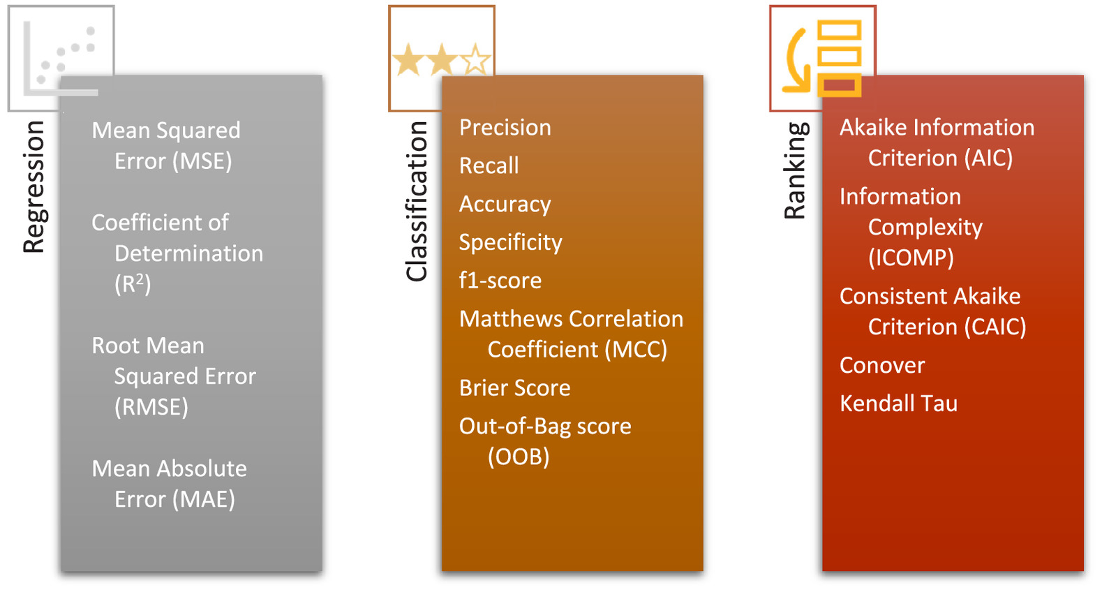
Evaluation Metrics in Regression Models
Mean squared error (MSE) measures the average squared difference between the predicted and actual values (Wallach and Goffinet 1989). The formula can be expressed aswhere = total number of data points; and and = representatives of actual and predicted values, respectively.
(4)
Coefficient of determination (CoD), also known as R-squared (), is a widely-used metric in assessing regression models and shows how good the regression model fits by showing it in a range of 0 (poor correlation) to 1 (perfect correlation) (Gelman et al. 2019). The equation of this metric is as follows:where is the mean of dependent variable.
(5)
Root mean squared error (RMSE) quantifies the average magnitude of prediction errors or residuals between the predicted and actual values (Chai and Draxler 2014). As RMSE squares the error, this metric is sensitive to outliers. The equation for this metric is as follows:
(6)
Mean absolute error (MAE) is a metric for measuring the average difference between actual and predicted values by calculating the absolute difference between these values (Chai and Draxler 2014). The formula for this metric is as follows:
(7)
Evaluation Metrics in Classification Models
Confusion matrix is a well-known table, widely used for evaluating the performance of classification models by comparing the number of predicted values to the actual values (Marom et al. 2010). It comprises four key values, as outlined as follows:
True Positive (TP): Representing number of correctly predicted positive values.
False Positive (FP): Representing number of incorrectly predicted positive values.
True Negative (TN): Representing number of correctly predicted negative values.
False Negative (FN): Representing number of incorrectly predicted negative values.
These four values used to calculate various performance metrics. Precision measures the proportion of correctly predicted positive instances out of all instances that were predicted as positive
(8)
Recall measures the proportion of correctly predicted positive instances out of all actual positive instances
(9)
Accuracy provides an assessment of how well the model performs in terms of correctly classifying instances
(10)
Specificity also measures the proportion of correctly predicted negative values out of all actual negative instances
(11)
F1-Score is a common metric, because of getting a harmonic average of both precision and recall providing a balanced measure of the models’ performance
(12)
Matthews correlation coefficient (MCC) is a metric that utilizes the four key values of the confusion matrix to provide a score ranging from to 1. A score of 1 indicates a perfect model, 0 represents a random prediction, and signifies a complete disagreement between the predicted and actual values (Chicco and Jurman 2020):
(13)
Brier score is defined as the mean squared difference between predicted probabilities and the actual values, in which lower scores indicate better predictability (Rufibach 2010)where = total number of instances in data; = actual binary value of 0 and 1; and = predicted probability of positive class.
(14)
Out-of-bag score (OOB) is a metric which estimates the model’s predictability on unseen data, derived from instances that were not used for training in each tree of ensemble models utilizing bagging strategy as RF (Fauzi 2018):where = actual known outcome of the th instance; = predicted outcome of the th instance using the trees that did not include it in their training subset; and = indicator function which returns 1 if the condition is true and 0 if false.
(15)
Area under the receiver operating characteristic curve (AUC-ROC) is a widely used evaluation metric for classification tasks. It assesses the performance of a classifier by measuring the true positive rate (TPR) and false positive rate (FPR) at various classification thresholds, and subsequently calculates the area under the curve. Its value is within range of 0 to 1, where 0.5 indicates a random selection and the higher the values, the stronger the classification (Huang et al. 2014).
Evaluation Metrics for Ranking
Concordance index (C-index) evaluates the accuracy and ranking ability of a model in distinguishing between relevant and non-relevant cases. It qualifies the degree of concordance and ranges between 0.5 and 1, in which C-index of 1 signifies the perfect concordance (Brentnall and Cuzick 2018).
Akaike information criterion (AIC) is a criterion for model selection and comparison which considers both models explanation ability and also the used number of parameters (Bozdogan 2000; Wagenmakers and Farrell 2004). The equation for calculation AIC is as follows:where = number of parameters of model; and = maximum likelihood estimate of the likelihood function of the model.
(16)
In addition to AIC, there are other criteria, such as information complexity (ICOMP) and consistent Akaike criterion (CAIC), that are employed for ranking the likelihoods obtained from models (Bozdogan 2009; Mohebbi et al. 2019).
The Conover-Iman test, a nonparametric test, utilizes the ranks of observations to determine a test statistic that quantifies the differences in the central tendency (location parameter) among various groups being compared (Iman and Conover 1982). The Kendall Tau rank correlation distance serves as a metric for quantifying the dissimilarity between two rankings. It offers insight into the extent of differences between the rankings. The Kendall Tau ranking ranges from 0 to 1, where a value of 0 signifies identical rankings, while a value of 1 represents the highest degree of disagreement between the rankings (Kendall 1938).
Appendix II. Summary of the Literature Review
| Reference | Clean water/wastewater | Objective | Main variables | Performance measure | Tree-based method(s) | Case studies | Length of WDN (km) | Failure data availability (year) | Material |
|---|---|---|---|---|---|---|---|---|---|
| Syachrani et al. (2012) | Wastewater | Real age | L; D; material; slope; pipe condition; problem type; etc. | MSE, MAE, RMSE | DT | Kansas, US | 95 (pressurized) + 3219 (gravity) | Not mentioned | VCP, PVC |
| Harvey and McBean (2014) | Wastewater | Individual pipe conditions (2 categories) | L; D; age; material; slope; road coverage; watermain breaks; land use; census tract; etc. | AUC, Youden (1950) J index | RF | City of Guelph, Ontario, Canada | 123 (gravity) | N/A | PVC, VCP, CP, AC, RC |
| Jilong (2014) | Water | Individual pipe conditions (3 categories) | D; age; material; pressure; distance to pump; distance to tank; load | AUC | C4.5 | Not mentioned | Not mentioned | Not mentioned | DI, CI, CP |
| Vitorino et al. (2014) | Wastewater | Pipe condition | L; D; age; material; zone; previous inspection; age at previous inspection | — | RF | — | — | — | DI, PVC, VCP, RPM, RCP |
| Rokstad and Ugarelli (2015) | Wastewater | Condition class (5 categories) | D; effluent type; construction era; road traffic; type of bedding soil; presence of trees | — | RF | Oslo municipality, Norway | 499 | 2002–2012 | CP, other |
| Wu et al. (2013) | Wastewater | Defect types | Image processing features | Correct classification rate (%), Recognition accuracy (%) | AdaBoost, RF, rotation forest, RotBoost | — | — | — | — |
| Santos et al. (2017) | Wastewater | Blockage failure for individual pipes | D; L; age; material; slope | % of avoided failures | DT, CART, RF, robust DT, robust forest | A sewer network in US | 3,803 | January 2012–May 2013 | PVC, DI, VCP, RPM |
| Myrans et al. (2018) | Wastewater | Pipe condition (Fault/normal) | GIST descriptor | Accuracy, FPR, AUC | RF | Wessex Water, UK | 5.5 | — | Brick, vitrified clay and concrete |
| Shi et al. (2018) | Water | Remaining wall thickness rating | Wall thickness; soil type; soil resistivity; soil pH; soil sulfite content; soil moisture; soil corrosivity | RMSE, | RF (ensembled with other ML methods) | City of Toronto | Not mentioned | January 1998–October 1999 | CI |
| Snider and McBean (2018) | Water | Time-to-failure for individual pipes | D; L; age; material; cement mortar lining year; cathodic protection year; pressure, break density, number of previously recorded failures, and break age for all previously recorded failures | RMSE, R | RF, XGB | A North American water utility | 339 | 1960–2017 | DI |
| Winkler et al. (2018) | Water | Failure/non-failure in pipe level | D; L; age; material; pressure; pipe type; etc. | AUC | DT, RF, AdaBoost, RUSBoost | A city in Austria | 851 | 1983 | PE, ST, PVC, DI, AC |
| Myrans et al. (2019) | Wastewater | Type of a detected fault | GIST descriptor | — | RF | Wessex Water, UK | 30 | — | Vitrified clay, PVC and brick |
| Shirzad and Safari (2019) | Water | Failure rate for classes of pipes | D; L; age; installation depth; average hydraulic pressure | RMSE, MAE, | RF | Mahabad city and Mashhad city, Iran | 139 and 579 (for each case study) | 1 year | PE and AC (for each case study) |
| Wols et al. (2018) | Water | Failure rate () | D; age; material; soil type; regional weather data | GB regression | Netherlands | 97,667 | January 2009–December 2014 | AC, GCI, DI, PVC, ST | |
| Almheiri et al. (2020) | Water | Time to failure for individual pipes | D; L; age; material | RMSE, MAE, | EDT | Sainte-Foy, Quebec | 432 | 1986–2001 | Grey CI, DI with/without lining, PVC, and hyprescon/concrete |
| Chen and Guikema (2020) | Water | Failure/non-failure in pipe level | D; L; age; material; average pressure; average flow; road proximity; soil corrosivity and frost potential; climatological data | Break capture versus length capture | DT, RF, GBT (+DBSCAN) | A WDN in Midwest US | 681 | 2008–2017 | CI, other |
| Giraldo-González and Rodríguez (2020) | Water | Failure/non-failure in pipe level | D; L; age; material; soil properties (contraction and expansion potential, moisture content); precipitation; land use; number of valves and hydrants connected to the pipe | Precision, recall, f-score, AUC | GBT | A WDN in Bogotá, Colombia | 1,819 | 2012–2018 | PVC, AC |
| Gorenstein et al. (2020) | Water | Ranking of pipe segments | L; age; material; etc. | RMSE, Conover, Kendall’s Tau | RF | Mekorot Company, Israel | Not mentioned | June 2016–December 2019 | Not mentioned |
| Konstantinou and Stoianov (2020) | Water | Annual number of failures in pipe segment and WDN level, probability of failure | D; L; age; material; maximum daily pressure and temperature; daily pressure and temperature range; corrosivity; fracture potential; etc. | AUC | RF, XGB | Not mentioned | 374 | 2003–2016 | — |
| Malek Mohammadi et al. (2020) | Wastewater | Pipe conditions (good/ critical) | D; L; age, material, flow rate, pipe depth, slope, soil type, pH, sulfate content, water table, soil hydraulic group, and soil corrosivity | ROC, confusion matrix | GBT | City of Tampa, Florida | 2,900 | N/A | — |
| Snider and McBean (2019) | Water | Time-to-next break for individual pipes | D; L; age; material; soil type; cement mortar lining year; cathodic protection year | RMSE, MAE, R, C-index | XGB | A WDN in Canada | 5,136 | 1960–2016 | CI |
| Snider and McBean (2020) | Water | Time-to-next break for individual pipes | — | C-index | XGB | A WDN in Canada | — | 1960–2016 | CI |
| Tavakoli et al. (2020) | Wastewater | Pipe condition | D; L; age; material; slope; depth of cover; age at the time of inspection; up/down elevation | Precision, recall, f1-score, AUC | RF | City of Los Angeles, US | — | N/A | VCP, AC, PVC, ST, CI, DI, etc. |
| Yang et al. (2020) | Water | Survival time of the pipes | Information of surrounding buildings; pipes lifetime; road width | Precision, ratio of risk | DT | Beijing, China | Not mentioned | January 2013–December 2016 | Not mentioned |
| Amini (2021) | Water | Probability of failure, age at first failure, current rate of failure | — | — | RF, XGB | Thirteen Canadian water utilities, including Barrie, Calgary, Halifax, etc. | — | — | CI, PVC, DI, AC, etc. |
| Aslani et al. (2021) | Water | Failure rate for pipes, pipe replacement ranking | D; L; age; material; available land and water; total precipitation; average temperature | RMSE, MAE, AIC, ICOMP, CAIC | RF, BRT | City of Tampa, Florida | Not mentioned | 2015–2020 | DI, CI, Galvanised Iron, PVC |
| Mazumder et al. (2021) | Oil and gas | Categorizing the pipes based on their failure pressure, into low, moderate, high and severe classes | D; wall thickness, defect depth; defect length; yield stress; ultimate tensile test; operating pressure | Precision, recall, accuracy | DT, RF, AdaBoost, XGBoost, LightBoost, CatBoost | 92 experimental test results for oil and gas pipelines, from literature | — | — | ST |
| Snider and McBean (2021) | Water | Time-to-next-break | D; L; age; material; pressure; soil type; cement mortar lining year; cathodic protection; age of pipes at 1st, 2nd, and 3rd last break | C-index, MAE | Random Survival Forest | A large water utility located in Canada | Not mentioned | CI, DI, AC, PVC | |
| Vaags (2021) | Water | LoF | D; L; age; material; soil type and resistivity; number of previous breaks; pressure; rainfall; temperature; flow; pump station proximity; water conductivity; etc. | RMSE, , C-index | XGB Survival Embedding, Random Survival Forest | 4 Utilities in Canada | 4,528, 1,570, 486, 1,473 | 64, 10, 45, 28 | PVC, DI, CI, AC, ST |
| Weeraddana et al. (2021) | Water | Failed/ not failed pipes | D; L; age; number of previous breaks; type | AUC | Random Survival Forest | Three major Australian states: VIC, NSW and QLD | — | 2000–2017 (VIC & NSW), 2013–2017 (QLD) | AC, CI, DI, PE, PVC, etc. |
| Assad and Bouferguene (2021) | Water | Pipe condition | D; L; age; material; number of previous breaks; annual average daily traffic; shallow main () | MAE, MAPE, RMSE, R | DT, RF, XGB, AdaBoost | Waterloo, Canada | 450 | — | PVC, DI, CI |
| Barton et al. (2022b) | Water | Probability of pipe failure | Number of previous breaks; L; D; age; material; water source; air frost; weekly soil moisture deficit and temperature; type, corrosivity, clay content, and shrink-swelling potential of soil | AUC, briers score, Mathews Correlation Coefficient | XGB | A UK WDN | 38,400 | 2015–2018 | PE, Iron, AC, PVC, ST, DI |
| Dimas et al. (2022) | Water | Probability of pipe failure | D; L; material; the main flagging (1 for main pipes, 0 for secondary/ tertiary pipes) | AUC | DT | Mourati zone, Greece; C-Town | Not mentioned | Not mentioned | Grey CI, seam ST, AC |
| Fan et al. (2021) | Water | Failed/ not failed pipes in a certain year | D; L; age; material; number of previous breaks; time-to-previous break; soil type; topographical data; census data; climate data | Precision, recall, accuracy, AUC | LightGBM | Cuyahoga County, Cleveland, US | 8,500 | Not mentioned | CI, DI, other |
| Liu et al. (2022) | Water | Failed/ not failed pipes in a certain year | D; L; age; material; qualification of construction enterprises, bridge pipe or not, road class, failure record | Accuracy, recall, specificity, AUC, out of bag score | RF | A WDN in Suzhou, China | 1,107 | Not mentioned | DI, CI, ST, PE, prestressed concrete cylinder pipe |
| Liu et al. (2022) | Oil | Failed/ not failed pipes | D; thickness; depth; slope; welding date, process, and company; max pressure; | Precision, recall, accuracy, AUC | XGB | — | — | — | — |
| Gioele (2022) | Water | — | D; L; age; material; average pressure | — | RF | City of Manresa, Spain | — | 2005–2019 | — |
| Robles-Velasco et al. (2020) | Water | — | — | — | — | — | — | — | — |
| Van Nguyen and Seidu (2022) | Wastewater | Pipe condition | D; L; age; material; slope; depth; rainfall, traffic; population; soil type; pipe type; groundwater; etc. | RMSE, MAE, | CART, RF, Extra Trees Regression, AdaBoost, GBT, Histogram-Based GBT | Oslo, Norway | 703 | — | PE, PVC, concrete, other |
| Abokifa and Sela (2023) | Water | Failure rate of sectors in WDN | D; L; age; fraction of materials by pipe length in each zone | RMSE, MAE | RF | A large metropolitan water utility in the US | 8,625 | September 2016–2019 | CI, PVC, DI, AC |
| Beig Zali et al. (2024) | Water | Likelihood of Failure in individual pipes | D; L; age; material; pressure; soil type | Precision, recall; AUC; 2 new measures | RF, XGB | A water utility in the UK | 32,800 | 2 | AC, CI, PVC, PE |
| Robles-Velasco et al. (2020) | Water | Failed/ not failed pipes in future | D; L; age; material; connections; mean and fluctuations of pressure; number of previous failures; time since last failure; soil type | Accuracy, recall, specificity, | RF | Seville, Spain | 3,800 | 2012–2018 | DI, CI, AC, PE, concrete, AC |
Data Availability Statement
All data, models, and code generated or used during the study appear in the published article.
Acknowledgments
This research has been funded by Datatecnics Corporation Limited and UKRI, under Knowledge Transfer Partnership (KTP) InnovateUK with Grant No. 12418.
References
Abokifa, A. A., and L. Sela. 2023. “Integrating spatial clustering with predictive modeling of pipe failures in water distribution systems.” Urban Water J. 20 (4): 465–476. https://doi.org/10.1080/1573062X.2023.2180393.
Afrifa, S., V. Vijayakumar, P. Appiahene, T. Zhang, and E. A. Domfeh. 2023. “Ensemble machine learning techniques for accurate and efficient detection of botnet attacks in connected computers.” Engineering 4 (1): 650–664. https://doi.org/10.3390/eng4010039.
Ag, P. V., and V. Varadarajan. 2021. “Estimating software development efforts using a Random Forest-based stacked ensemble approach.” Electronics 10 (10): 1195. https://doi.org/10.3390/electronics10101195.
Almheiri, Z., M. A. Meguid, and T. Zayed. 2020. “Intelligent approaches for predicting failure of water mains.” J. Pipeline Syst. Eng. Pract. 11 (4): 04020044. https://doi.org/10.1061/(ASCE)PS.1949-1204.0000485.
Alvisi, S., and M. Franchini. 2010. “Comparative analysis of two probabilistic pipe breakage models applied to a real water distribution system.” Civ. Eng. Environ. Syst. 27 (1): 1–22. https://doi.org/10.1080/10286600802224064.
Amini, M. 2021. “Application of machine learning algorithms to the prediction of water main deterioration.” Master thesis, Dept. of Building, Civil, and Environmental Engineering, Concordia Univ.
Anjum, M., K. Khan, W. Ahmad, A. Ahmad, M. Amin, and A. Nafees. 2022. “Application of ensemble machine learning methods to estimate the compressive strength of fiber-reinforced nano-silica modified concrete.” Polymers 14 (18): 3906. https://doi.org/10.3390/polym14183906.
Aslani, B., S. Mohebbi, and H. Axthelm. 2021. “Predictive analytics for water main breaks using spatiotemporal data.” Urban Water J. 18 (6): 433–448. https://doi.org/10.1080/1573062X.2021.1893363.
Asnaashari, A., E. A. McBean, I. Shahrour, and H. Bonakdari. 2009. “Prediction of watermain failure frequencies using multiple and Poisson regression.” Water Sci. Technol. Water Supply 9 (1): 9–19. https://doi.org/10.2166/ws.2009.020.
Assad, A., and A. Bouferguene. 2021. “Data mining algorithms for water main condition prediction—Comparative analysis.” J. Water Resour. Plann. Manage. 148 (2): 04021101. https://doi.org/10.1061/(ASCE)WR.1943-5452.0001512.
Barton, N. A., S. H. Hallett, S. Jude, and T. Tran. 2022a. “An evolution of statistical pipe failure models for drinking water networks: A targeted review.” Water Sci. Technol. Water Supply 22 (4): 3784–3813. https://doi.org/10.2166/ws.2022.019.
Barton, N. A., S. H. Hallett, S. Jude, and T. Tran. 2022b. “Predicting the risk of pipe failure using gradient boosted decision trees and weighted risk analysis.” Clean Water 5 (1). https://doi.org/10.1038/s41545-022-00165-2.
Batra, M., and R. Agrawal. 2017. “Comparative analysis of decision tree algorithms.” In Advances in intelligent systems and computing, 31–36. New York: Springer.
Beig Zali, R., M. Latifi, A. A. Javadi, and R. Farmani. 2024. “Semi-supervised clustering approach for pipe failure prediction with imbalanced dataset.” J. Water Resour. Plann. Manage. 150 (2): 04023078. https://doi.org/10.1061/JWRMD5.WRENG-6263.
Berardi, L., O. Giustolisi, Z. Kapelan, and D. Savic. 2008. “Development of pipe deterioration models for water distribution systems using EPR.” J. Hydroinf. 10 (2): 113–126. https://doi.org/10.2166/hydro.2008.012.
Bozdogan, H. 2000. “Akaike’s information criterion and recent developments in information complexity.” J. Math. Psychol. 44 (1): 62–91. https://doi.org/10.1006/jmps.1999.1277.
Bozdogan, H. 2009. “A new class of information complexity (ICOMP) criteria with an application to customer profiling and segmentation.” DergiPark. Istanbul Univ. Accessed April 4, 2024. https://dergipark.org.tr/tr/pub/iuisletme/issue/9248/115706.
Brédart, X., E. Séverin, and D. Veganzones. 2021. “Human resources and corporate failure prediction modeling: Evidence from Belgium.” J. Forecasting 40 (7): 1325–1341. https://doi.org/10.1002/for.2770.
Breiman, L. 1984. “Classification and regression trees.” Biometrics 40 (3): 874. https://doi.org/10.2307/2530946.
Breiman, L. 2001. “Random forests.” Mach. Learn. 45 (Mar): 5–32. https://doi.org/10.1023/A:1010933404324.
Brentnall, A. R., and J. Cuzick. 2018. “Use of the concordance index for predictors of censored survival data.” Stat. Methods Med. Res. 27 (8): 2359–2373. https://doi.org/10.1177/0962280216680245.
Chai, T., and R. R. Draxler. 2014. “Root mean square error (RMSE) or mean absolute error (MAE)?—Arguments against avoiding RMSE in the literature.” Geosci. Model Dev. 7 (3): 1247–1250. https://doi.org/10.5194/gmd-7-1247-2014.
Chawla, N. V., K. W. Bowyer, L. J. Hall, and W. P. Kegelmeyer. 2002. “SMOTE: Synthetic minority over-sampling technique.” J. Artif. Intell. Res. 16 (Mar): 321–357. https://doi.org/10.1613/jair.953.
Chen, T. C., and S. D. Guikema. 2020. “Prediction of water main failures with the spatial clustering of breaks.” Reliab. Eng. Syst. Saf. 203 (Mar): 107108. https://doi.org/10.1016/j.ress.2020.107108.
Chicco, D., and G. Jurman. 2020. “The advantages of the Matthews correlation coefficient (MCC) over F1 score and accuracy in binary classification evaluation.” BMC Genomics 21 (1): 1–13. https://doi.org/10.1186/s12864-019-6413-7.
Coadou, Y. 2022. “Boosted decision trees.” In World scientific ebooks, 9–58. Singapore: World Scientific. https://doi.org/10.1142/9789811234033_0002.
Dawood, T., E. Elwakil, H. M. Novoa, and J. A. Delgado. 2020. “Water pipe failure prediction and risk models: State-of-the-art review.” Can. J. Civ. Eng. 47 (10): 1117–1127. https://doi.org/10.1139/cjce-2019-0481.
Debón, A., A. Carrión, E. Cabrera, and H. E. G. Solano. 2010. “Comparing risk of failure models in water supply networks using ROC curves.” Reliab. Eng. Syst. Saf. 95 (1): 43–48. https://doi.org/10.1016/j.ress.2009.07.004.
Delnaz, A., F. Nasiri, and S. S. Li. 2023. “Asset management analytics for urban water mains: A literature review.” Environ. Syst. Res. 12 (1): 12. https://doi.org/10.1186/s40068-023-00287-7.
Dimas, P., D. Nikolopoulos, and C. Makropoulos. 2022. “Simulation framework for pipe failure detection and replacement scheduling.” Optimization 21 (1): 37. https://doi.org/10.3390/environsciproc2022021037.
Economou, T., Z. Kapelan, and T. C. Bailey. 2012. “On the prediction of underground water pipe failures: Zero inflation and pipe-specific effects.” J. Hydroinf. 14 (4): 872–883. https://doi.org/10.2166/hydro.2012.144.
Fan, X., X. Wang, and X. Zhang. 2021. “Machine learning based water pipe failure prediction: The effects of engineering, geology, climate and socio-economic factors.” Reliab. Eng. Syst. Saf. 219 (Mar): 108185. https://doi.org/10.1016/j.ress.2021.108185.
Farhadi, B., and R. C. K. Wong. 2014. “Numerical modeling of pipe-soil interaction under transverse direction.” In Proc., Int. Pipeline Conf. New York: ASME.
Farmani, R., K. Kakoudakis, K. Behzadian, and D. Butler. 2017. “Pipe failure prediction in water distribution systems considering static and dynamic factors.” Procedia Eng. 186 (May): 117–126. https://doi.org/10.1016/j.proeng.2017.03.217.
Fauzi, M. A. 2018. “Random forest approach for sentiment analysis in Indonesian language.” Indones. J. Electr. Eng. Comput. Sci. 12 (1): 46. https://doi.org/10.11591/ijeecs.v12.i1.pp46-50.
Fiosina, J., P. Sievers, M. Drache, and S. Beuermann. 2023. Polymer reaction engineering meets explainable machine learning. Cambridge, UK: Cambridge Open Engage.
Francis, R. A., S. D. Guikema, and L. R. Henneman. 2014. “Bayesian belief networks for predicting drinking water distribution system pipe breaks.” Reliab. Eng. Syst. Saf. 130 (May): 1–11. https://doi.org/10.1016/j.ress.2014.04.024.
Freund, Y., and R. E. Schapire. 1996. “Experiments with a new boosting algorithm.” In Proc., 13th Int. Conf. on Machine Learning, 148–156. San Francisco: Morgan Kaufmann Publishers Inc.
Friedman, J. H. 2002. “Stochastic gradient boosting.” Comput. Stat. Data Anal. 38 (4): 367–378. https://doi.org/10.1016/S0167-9473(01)00065-2.
Ganaie, M., M. Hu, M. Tanveer, and P. N. Suganthan. 2021. “Ensemble deep learning: A review.” Eng. Appl. Artif. Intell. 115 (Oct): 105151. https://doi.org/10.1016/j.engappai.2022.105151.
Gelman, A., B. Goodrich, J. Gabry, and A. Vehtari. 2019. “R-squared for Bayesian regression models.” Am. Stat. 73 (3): 307–309. https://doi.org/10.1080/00031305.2018.1549100.
Geurts, P., D. Ernst, and L. Wehenkel. 2006. “Extremely randomized trees.” Mach. Learn. 63 (1): 3–42. https://doi.org/10.1007/s10994-006-6226-1.
Gioele, B. P. 2022. “A new machine learning approach to support asset management in water distribution networks.” Master thesis, School of Industrial, Aerospace and Audiovisual Engineering, Universitat Politècnica de Catalunya–BarcelonaTech, Terrassa.
Giraldo-González, M. M., and J. M. Rodríguez. 2020. “Comparison of statistical and machine learning models for pipe failure modeling in water distribution networks.” Water 12 (4): 1153. https://doi.org/10.3390/w12041153.
Gorenstein, A., M. Kalech, D. F. Hanusch, and S. Hassid. 2020. “Pipe fault prediction for water transmission mains.” Water 12 (10): 2861. https://doi.org/10.3390/w12102861.
Gupta, N. S., Y. Mohta, K. Heda, R. Armaan, B. Valarmathi, and G. Arulkumaran. 2023. “Prediction of air quality index using machine learning techniques: A comparative analysis.” J Environ. Public Health 2023 (May): 1–26. https://doi.org/10.1155/2023/4916267.
Hancock, J. F., and T. M. Khoshgoftaar. 2020. “CatBoost for big data: An interdisciplinary review.” J. Big Data 7 (1): 94. https://doi.org/10.1186/s40537-020-00369-8.
Harvey, R. R., and E. A. McBean. 2014. “Predicting the structural condition of individual sanitary sewer pipes with random forests.” Can. J. Civ. Eng. 41 (4): 294–303. https://doi.org/10.1139/cjce-2013-0431.
Hasani, S., and H. R. Nasiri. 2021. “COV-ADSX: An automated detection system using X-ray images, deep learning, and XGBoost for COVID-19.” Software Impacts 11 (May): 100210. https://doi.org/10.1016/j.simpa.2021.100210.
Hastuti, R., I. Waspada, P. W. Wirawan, and N. Bahtiar. 2020. “Designing computer-assisted problem-based learning (CAPBL) environment for performance analysis of isolation forest algorithm.” J. Phys. 1524 (Apr): 012103. https://doi.org/10.1088/1742-6596/1524/1/012103.
Huang, G., S. Song, J. N. D. Gupta, and C. Y. Wu. 2014. “Semi-supervised and unsupervised extreme learning machines.” IEEE Trans. Cybern. 44 (12): 2405–2417. https://doi.org/10.1109/TCYB.2014.2307349.
Iman, R. L., and W. J. Conover. 1982. “A distribution-free approach to inducing rank correlation among input variables.” Commun. Stat.- Simul. Comput. 11 (3): 311–334. https://doi.org/10.1080/03610918208812265.
Ishwaran, H., U. B. Kogalur, E. H. Blackstone, and M. S. Lauer. 2008. “Random survival forests.” Ann. Appl. Stat. 2 (3): 124. https://doi.org/10.1214/08-AOAS169.
Jafarzadeh, H., M. Mahdianpari, E. W. Gill, F. Mohammadimanesh, and S. Homayouni. 2021. “Bagging and boosting ensemble classifiers for classification of multispectral, hyperspectral and PolSAR data: A comparative evaluation.” Remote Sens. 13 (21): 4405. https://doi.org/10.3390/rs13214405.
Jagtiani, J., and C. E. Henderson. 2010. “Can banks circumvent minimum capital requirements? The case of mortgage portfolios under Basel II.” In Social science research network. Philadelphia: Federal Reserve Bank of Philadelphia.
Jain, V., and K. L. Kashyap. 2022. “Multilayer hybrid ensemble machine learning model for analysis of Covid-19 vaccine sentiments.” J. Intell. Fuzzy Syst. 43 (5): 6307–6319. https://doi.org/10.3233/JIFS-220279.
Jilong, S. 2014. “Decision tree classification model in water supply network.” CUNY Academic Works. Accessed March 4, 2024. https://academicworks.cuny.edu/cc_conf_hic/65/.
Jin, W., M. Fatehi, K. Abhishek, M. Mallya, B. Toyota, and G. Hamarneh. 2019. “Artificial intelligence in glioma imaging: Challenges and advances.” J. Neural Eng. 17 (2): 021002. https://doi.org/10.1088/1741-2552/ab8131.
Kaczałek, B., and A. Borkowski. 2016. “Urban road detection in airborne laser scanning point cloud using random forest algorithm.” ISPRS Ann. Photogramm. Remote Sens. Spatial Inf. Sci. 41 (Jun): 255–259. https://doi.org/10.5194/isprs-archives-xli-b3-255-2016.
Kakoudakis, K., K. Behzadian, R. Farmani, and D. Butler. 2017. “Pipeline failure prediction in water distribution networks using evolutionary polynomial regression combined with K-means clustering.” Urban Water J. 14 (7): 737–742. https://doi.org/10.1080/1573062X.2016.1253755.
Kakoudakis, K., R. Farmani, and D. Butler. 2018. “Pipeline failure prediction in water distribution networks using weather conditions as explanatory factors.” J. Hydroinf. 20 (5): 1191–1200. https://doi.org/10.2166/hydro.2018.152.
Kang, M., M. Kim, and J. Lee. 2010. “Analysis of rigid pavement distresses on interstate highway using decision tree algorithms.” KSCE J. Civ. Eng. 14 (2): 123–130. https://doi.org/10.1007/s12205-010-0123-7.
Kass, G. V. 1980. “An exploratory technique for investigating large quantities of categorical data.” Appl. Stat. 20 (2): 8. https://doi.org/10.2307/2986296.
Katterbauer, K., H. Syed, S. Y. Genç, and L. Cleenewerck. 2022. “Environmental compliance and financial performance of Shariah-compliant enterprises—A data-driven analysis.” Revista De Gestão Social E Ambiental 16 (2): e03043. https://doi.org/10.24857/rgsa.v16n2-025.
Ke, G., Q. Meng, T. Finley, T. Wang, W. Chen, W. Ma, Q. Ye, and T. Liu. 2017. “LightGBM: A highly efficient gradient boosting decision tree.” Adv. Neural Inf. Proc. Syst. 30 (Mar): 3149–3157. https://doi.org/10.5555/3294996.3295074.
Kendall, M. 1938. “A new measure of rank correlation.” Biometrika 30 (1/2): 81–89. https://doi.org/10.2307/2332226.
Kerwin, S. M., B. G. De Soto, B. T. Adey, K. Sampatakaki, and H. Heller. 2020. “Combining recorded failures and expert opinion in the development of ANN pipe failure prediction models.” Sustainable Resilient Infrastruct. 8 (1): 86–108. https://doi.org/10.1080/23789689.2020.1787033.
Kettler, A. J., and I. C. Goulter. 1985. “An analysis of pipe breakage in urban water distribution networks.” Can. J. Civ. Eng. 12 (2): 286–293. https://doi.org/10.1139/l85-030.
Kim, H. J., H. B. Bae, J. W. Jeon, Y. R. Ham, K. Y. Na, K. Lee, Y. K. Hyon, and D. S. Choi. 2021. “A novel approach to dry weight adjustments for dialysis patients using machine learning.” PLoS One 16 (4): e0250467. https://doi.org/10.1371/journal.pone.0250467.
Kirmeyer, G. J., W. Richards, and C. D. Smith. 1994. Assessment of water distribution systems and associated research needs. Denver: American Water Works Association.
Kleiner, Y., and B. Rajani. 2001. “Comprehensive review of structural deterioration of water mains: Statistical models.” Urban Water 3 (3): 131–150. https://doi.org/10.1016/S1462-0758(01)00033-4.
Kleiner, Y., and B. Rajani. 2010. “I-WARP: Individual water main renewal planner.” Drinking Water Eng. Sci. 3 (1): 71–77. https://doi.org/10.5194/dwes-3-71-2010.
Kong, Y., B. Yan, Y. Liu, H. Leung, and X. Peng. 2021. “Feature-level fusion of polarized SAR and optical images based on random forest and conditional random fields.” Remote Sens. 13 (7): 1323. https://doi.org/10.3390/rs13071323.
Konstantinou, C., and I. Stoianov. 2020. “A comparative study of statistical and machine learning methods to infer causes of pipe breaks in water supply networks.” Urban Water J. 17 (6): 534–548. https://doi.org/10.1080/1573062X.2020.1800758.
Kulkarni, V., and P. K. Sinha. 2012. “Pruning of Random Forest classifiers: A survey and future directions.” In Proc., 2012 Int. Conf. on Data Science and Engineering (ICDSE), 64–68. New York: IEEE.
Kumar, G. D. 2019. “Tree-based modeling techniques.” In IGI Global eBooks, 1–18. Pennsylvania: IGI Global.
Kumbhakarna, V. M., S. B. Kulkarni, and A. Dhawale. 2020. “NLP algorithms endowed for automatic extraction of information from unstructured free-text reports of radiology monarchy.” Engineering 9 (12): 338–343. https://doi.org/10.35940/ijitee.l8009.1091220.
Kutyłowska, M. 2018. “Application of K-nearest neighbours method for water pipes failure frequency assessment.” In Vol. 59 of Proc., E3S Web of Conf., 00021. Les Ulis, France: EDP Sciences.
Kutyłowska, M. 2019. “Forecasting failure rate of water pipes.” Water Sci. Technol. 19 (1): 264–273. https://doi.org/10.2166/ws.2018.078.
Kwon, S. K., E. Hyun, J. H. Lee, J. Lee, and S. H. Son. 2017. “Detection scheme for a partially occluded pedestrian based on occluded depth in lidar–radar sensor fusion.” Opt. Eng. 56 (11): 1. https://doi.org/10.1117/1.OE.56.11.113112.
Larin, O., E. Barkanov, and O. Vodka. 2016. “Prediction of reliability of the corroded pipeline considering the randomness of corrosion damage and its stochastic growth.” Eng. Fail. Anal. 66 (May): 60–71. https://doi.org/10.1016/j.engfailanal.2016.03.022.
Laskov, P., P. Düssel, C. Schäfer, and K. Rieck. 2005. “Learning intrusion detection: Supervised or unsupervised?” In Vol. 3617 of Image analysis and processing—ICIAP 2005. ICIAP 2005. Lecture notes in computer science, edited by F. Roli and S. Vitulano, 50–57. Berlin: Springer. https://doi.org/10.1007/11553595_6.
Lee, C. 2021. “Using classification tree models to determine course placement.” Educ. Meas. 41 (2): 82–89. https://doi.org/10.1111/emip.12470.
Lee, S., and C. Lee. 2015. “Application of decision-tree model to groundwater productivity-potential mapping.” Sustainability 7 (10): 13416–13432. https://doi.org/10.3390/su71013416.
Le Gat, Y. 2008. “Modelling the deterioration process of drainage pipelines.” Urban Water J. 5 (2): 97–106. https://doi.org/10.1080/15730620801939398.
Le Gat, Y. 2013. “Extending the Yule process to model recurrent pipe failures in water supply networks.” Urban Water J. 11 (8): 617–630. https://doi.org/10.1080/1573062X.2013.783088.
Li, L., S. Wang, and G. Gong. 2011. “Research on decision tree algorithm based on information entropy.” Adv. Mater. Res. 267 (May): 732–737. https://doi.org/10.4028/www.scientific.net/amr.267.732.
Li, Y., and S. Yin. 2023. “User cold start recommendation system based on hofstede cultural theory.” Int. J. Web Serv. Res. 20 (1): 1–17. https://doi.org/10.4018/IJWSR.321199.
Liu, W., B. Wang, and Z. Song. 2022. “Failure prediction of municipal water pipes using machine learning algorithms.” Water Resour. Manage. 36 (4): 1271–1285. https://doi.org/10.1007/s11269-022-03080-w.
Liu, X., H. Huang, and W. Xu. 2004. “A contribution to decision tree construction based on rough set theory.” In Lecture notes in computer science. New York: Springer.
Loft Data Science Team. 2021. “XGBSE: XGBoost survival embeddings.” Accessed April 4, 2024. https://github.com/loft-br/xgboost-survival-embeddings.
Loh, W. Y., and Y. S. Shih. 1997. “Split selection methods for classification trees.” Statistica Sin. 7 (4): 815–840.
Luo, Y., and M. Spindler. 2016. High-dimensional L2 boosting: Rate of convergence. Ithaca, NY: Cornell Univ.
Mahmoodian, M., and C. Li. 2015. “Structural integrity of corrosion-affected cast iron water pipes using a reliability-based stochastic analysis method.” Struct. Infrastruct. Eng. 12 (10): 1356–1363. https://doi.org/10.1080/15732479.2015.1117114.
Malek Mohammadi, M. M., M. Najafi, N. Salehabadi, R. Serajiantehrani, and V. Kaushal. 2020. “Predicting condition of sanitary sewer pipes with gradient boosting tree.” In Pipelines 2020, 80–89. Reston, VA: ASCE.
Mallick, J., S. Pal, and M. Ahmed. 2022. “Combining high resolution input and stacking ensemble machine learning algorithms for developing robust groundwater potentiality models in Bisha watershed, Saudi Arabia.” Appl. Water Sci. 12 (4): 77. https://doi.org/10.1007/s13201-022-01599-2.
Marom, N. D., L. Rokach, and A. Shmilovici. 2010. “Using the confusion matrix for improving ensemble classifiers.” In Proc., 2010 IEEE 26th Convention of Electrical and Electronics Engineers in Israel, 000555–000559. New York: IEEE.
Mayr, A., H. Binder, O. Gefeller, and M. Schmid. 2014. “The evolution of boosting algorithms.” Methods Inf. Med. 53 (6): 419–427. https://doi.org/10.48550/arXiv.1403.1452.
Mazumder, R. K., A. M. Salman, and Y. Li. 2021. “Failure risk analysis of pipelines using data-driven machine learning algorithms.” Struct. Saf. 89 (May): 102047. https://doi.org/10.1016/j.strusafe.2020.102047.
Mehmood, K., H. A. Hassan, A. Raza, A. Altalbe, and H. Farooq. 2019. “Optimal power generation in energy-deficient scenarios using bagging ensembles.” IEEE Access 7 (May): 155917–155929. https://doi.org/10.1109/ACCESS.2019.2946640.
Mishina, Y., R. Murata, Y. Yamauchi, T. Yamashita, and H. Fujiyoshi. 2015. “Boosted random forest.” IEICE Trans. Inf. Syst. 98 (9): 1630–1636. https://doi.org/10.1587/transinf.2014OPP0004.
Modabbernia, A., H. C. Whalley, D. C. Glahn, P. M. Thompson, R. S. Kahn, and S. Frangou. 2022. “Systematic evaluation of machine learning algorithms for neuroanatomically-based age prediction in youth.” Hum. Brain Mapp. 43 (17): 5126–5140. https://doi.org/10.1002/hbm.26010.
Mohebbi, S., E. Pamukçu, and H. Bozdogan. 2019. “A new data adaptive elastic net predictive model using hybridized smoothed covariance estimators with information complexity.” J. Stat. Comput. Simul. 89 (6): 1060–1089. https://doi.org/10.1080/00949655.2019.1576683.
Muhammad, F. T., H. Chen, M. Kashif, A. L. Noman, K. Asad, and S. Muhammad. 2020. “Short term load forecasting using bootstrap aggregating based ensemble artificial neural network.” Recent Adv. Electr. Electron. Eng. 13 (7): 980–992. https://doi.org/10.2174/2213111607666191111095329.
Murugathasan, P., A. S. Dhar, and B. Hawlader. 2021. “An experimental and numerical investigation of pullout behavior of ductile iron water pipes buried in sand.” Can. J. Civ. Eng. 48 (2): 134–143. https://doi.org/10.1139/cjce-2019-0366.
Myrans, J., R. M. Everson, and Z. Kapelan. 2019. “Automated detection of fault types in CCTV sewer surveys.” J. Hydroinf. 21 (1): 153–163. https://doi.org/10.2166/hydro.2018.073.
Myrans, J., Z. Kapelan, and R. M. Everson. 2018. “Combining classifiers to detect faults in wastewater networks.” Water Sci. Technol. 77 (9): 2184–2189. https://doi.org/10.2166/wst.2018.131.
Nanda, S. S., S. Mishra, and S. Mohanty. 2011. “Oriya language text mining using C5.0 algorithm.” Int. J. Comput. Sci. Inf. Technol. 2 (1): 551–554.
Nishio, M., M. Nishizawa, O. Sugiyama, R. Kojima, M. Yakami, T. Kuroda, and K. Togashi. 2018. “Computer-aided diagnosis of lung nodule using gradient tree boosting and Bayesian optimization.” PLoS One 13 (4): e0195875. https://doi.org/10.1371/journal.pone.0195875.
Nishiyama, M., and Y. Filion. 2014. “Forecasting breaks in cast iron water mains in the city of Kingston with an artificial neural network model.” Can. J. Civ. Eng. 41 (10): 918–923. https://doi.org/10.1139/cjce-2014-0114.
Nnebedum, V. I. 2012. “The adaptability of decision tree method in mining industry safety data.” Int. J. Comput. Appl. Technol. 50 (22): 4–10. https://doi.org/10.5120/7932-1080.
Nunes, R., E. Arraut, and M. A. Da Silva Pimentel. 2023. “Risk assessment model for the renewal of water distribution networks: A practical approach.” Water 15 (8): 1509. https://doi.org/10.3390/w15081509.
Ogunleye, J. O. 2022. “Predictive data analysis using linear regression and random forest.” In Data integrity and data governance. London: IntechOpen.
Ono, S., and T. Goto. 2022. “Introduction to supervised machine learning in clinical epidemiology.” Ann. Clin. Epidemiol. 4 (3): 63–71. https://doi.org/10.37737/ace.22009.
Quinlan, J. R. 1990. “Probabilistic decision trees.” In Machine learning, edited by Y. Kodratoff and R. S. Michalski, 140–152. San Mateo, CA: Morgan Kaufmann.
Quinlan, J. R. 1992. C4.5 programs for machine learning. San Mateo, CA: Morgan Kaufmann.
Rahim, A. I. A., M. H. W. Ibrahim, S. Chua, and K. I. Musa. 2021. “Hospital facebook reviews analysis using a machine learning sentiment analyzer and quality classifier.” Healthcare 9 (12): 1679. https://doi.org/10.3390/healthcare9121679.
Rajani, B., and Y. Kleiner. 2001. “Comprehensive review of structural deterioration of water mains: Physically based models.” Urban Water 3 (3): 151–164. https://doi.org/10.1016/S1462-0758(01)00032-2.
Rajani, B., and J. Makar. 2000. “A methodology to estimate remaining service life of grey cast iron water mains.” Can. J. Civ. Eng. 27 (6): 1259–1272. https://doi.org/10.1139/l00-073.
Rajani, B., C. Zhan, and S. Kuraoka. 1996. “Pipe-soil interaction analysis of jointed water mains.” Can. Geotech. J. 33 (3): 393–404. https://doi.org/10.1139/t96-061.
Robles-Velasco, A., P. Cortés, J. Muñuzuri, and L. Onieva. 2020. “Prediction of pipe failures in water supply networks using logistic regression and support vector classification.” Reliab. Eng. Syst. Saf. 196 (Apr): 106754. https://doi.org/10.1016/j.ress.2019.106754.
Rokstad, M. M., and R. M. Ugarelli. 2015. “Evaluating the role of deterioration models for condition assessment of sewers.” J. Hydroinf. 17 (5): 789–804. https://doi.org/10.2166/hydro.2015.122.
Røstum, J. 2000. “Statistical modelling of pipe failures in water networks.” Ph.D. thesis, Dept. of Hydraulic and Environmental Engineering, Norwegian Univ. of Science and Technology.
Rufibach, K. 2010. “Use of brier score to assess binary predictions.” J. Clin. Epidemiol. 63 (8): 938–939. https://doi.org/10.1016/j.jclinepi.2009.11.009.
Sægrov, S., and W. Schilling. 2002. “Computer aided rehabilitation of sewer and storm water.” In Proc., 9th Int. Conf. on Urban Drainage. Reston, VA: Urban Water Resources Research Council of the Environmental Water Resources Institute of ASCE. https://doi.org/10.1061/40644(2002)88.
Saez, Y., A. Baldominos, and P. Isasi. 2016. “A comparison study of classifier algorithms for cross-person physical activity recognition.” Sensors 17 (12): 66. https://doi.org/10.3390/s17010066.
Sander, J., M. Ester, H. P. Kriegel, and X. Xu. 1998. “Density-based clustering in spatial databases: The algorithm GDBSCAN and its applications.” Data Min. Knowl. Discovery 2 (2): 169–194. https://doi.org/10.1023/A:1009745219419.
Santos, P. A., C. Amado, S. T. Coelho, and J. P. Leitão. 2017. “Stochastic data mining tools for pipe blockage failure prediction.” Urban Water J. 14 (4): 343–353. https://doi.org/10.1080/1573062X.2016.1148178.
Schapire, R. E. 1999. “A brief introduction to boosting.” In Vol. 2 of Proc., Int. Joint Conf. on Artificial Intelligence, 1401–1406. San Francisco: Morgan Kaufmann Publishers Inc.
Scheidegger, A., J. P. Leitão, and L. Scholten. 2015. “Statistical failure models for water distribution pipes–A review from a unified perspective.” Water Res. 83 (Mar): 237–247. https://doi.org/10.1016/j.watres.2015.06.027.
Seica, M. V., and J. A. Packer. 2004. “Finite element evaluation of the remaining mechanical strength of deteriorated cast iron pipes.” J. Eng. Mater. Technol. 126 (1): 95–102. https://doi.org/10.1115/1.1631027.
Seiffert, C., T. M. Khoshgoftaar, J. Van Hulse, and A. Napolitano. 2010. “RUSBoost: A hybrid approach to alleviating class imbalance.” IEEE Trans. Syst. Man Cybern. Part A Syst. Humans 40 (1): 185–197. https://doi.org/10.1109/TSMCA.2009.2029559.
Selcuk, S. 2016. “Predictive maintenance, its implementation and latest trends.” Proc. Inst. Mech. Eng., Part B: J. Eng. Manuf. 231 (9): 1670–1679. https://doi.org/10.1177/0954405415601640.
Shahhosseini, M., and G. Hu. 2020. “Improved weighted random forest for classification problems.” In Vol. 1301 of Progress in intelligent decision science. IDS 2020. Advances in intelligent systems and computing, edited by T. Allahviranloo, S. Salahshour, and N. Arica, 42–56. Cham, Switzerland: Springer.
Shamir, U., and C. D. D. Howard. 1979. “An analytic approach to scheduling pipe replacement.” J. Am. Water Works Assn. 71 (5): 248–258. https://doi.org/10.1002/j.1551-8833.1979.tb04345.x.
Shi, F., Y. Liu, Z. Liu, and E. Li. 2018. “Prediction of pipe performance with stacking ensemble learning based approaches.” J. Intell. Fuzzy Syst. 34 (6): 3845–3855. https://doi.org/10.3233/JIFS-169556.
Shi, F., Z. Liu, and E. Li. 2017. “Prediction of pipe performance with ensemble machine learning based approaches.” In Proc., 2017 Int. Conf. on Sensing, Diagnostics, Prognostics, and Control (SDPC), Shanghai, China, 408–414. New York: IEEE. https://doi.org/10.1109/SDPC.2017.84.
Shirzad, A., and M. J. S. Safari. 2019. “Pipe failure rate prediction in water distribution networks using multivariate adaptive regression splines and random forest techniques.” Urban Water J. 16 (9): 653–661. https://doi.org/10.1080/1573062X.2020.1713384.
Siregar, M. U., P. W. Hardjita, F. A. Asdin, D. Wardani, A. Wijayanto, Y. Yunitasari, and M. Anshari. 2022. “Housing price prediction using a hybrid genetic algorithm with extreme gradient boosting.” In Proc., IC3INA ′22: Proc., 2022 Int. Conf. on Computer, Control, Informatics and Its Applications. New York: Association for Computing Machinery.
Smith, H., P. J. Biggs, N. P. French, A. Smith, and J. Marshall. 2022. “Lost in the forest.” In bioRxiv (cold spring harbor laboratory). New York: bioRxiv—Bioinformatics.
Snider, B., and E. A. McBean. 2018. “Improving time to failure predictions for water distribution systems using extreme gradient boosting algorithm: (049).” Accessed March 4, 2024. https://ojs.library.queensu.ca/index.php/wdsa-ccw/article/view/12099.
Snider, B., and E. A. McBean. 2019. “Improving urban water security through pipe-break prediction models: Machine learning or survival analysis.” J. Environ. Eng. 146 (3): 04019129. https://doi.org/10.1061/(ASCE)EE.1943-7870.0001657.
Snider, B., and E. A. McBean. 2020. “Watermain breaks and data: The intricate relationship between data availability and accuracy of predictions.” Urban Water J. 17 (2): 163–176. https://doi.org/10.1080/1573062X.2020.1748664.
Snider, B., and E. A. McBean. 2021. “Combining machine learning and survival statistics to predict remaining service life of watermains.” J. Infrastruct. Syst. 27 (3): 04021019. https://doi.org/10.1061/(ASCE)IS.1943-555X.0000629.
Song, J., Y. Wang, M. Yang, and R. Liu. 2020. “The application of decision tree model in differential diagnosis of myelodysplastic syndrome and aplastic anemia.” Indian J. Pharm. Sci. 83 (6): 50–58. https://doi.org/10.36468/pharmaceutical-sciences.spl.399.
St. Clair, A. M., and S. K. Sinha. 2012. “State-of-the-technology review on water pipe condition, deterioration and failure rate prediction models!” Urban Water J. 9 (2): 85–112. https://doi.org/10.1080/1573062x.2011.644566.
Suriyanarayanan, C., and S. Kunasekaran. 2020. “Anomaly detection using machine learning techniques.” Malaya J. Mat. 8 (4): 2144–2148. https://doi.org/10.26637/MJM0804/0139.
Syachrani, S., H. M. Jeong, and C. S. Chung. 2012. “Decision tree–Based deterioration model for buried wastewater pipelines.” J. Perform. Constr. Facil. 27 (5): 633–645. https://doi.org/10.1061/(ASCE)CF.1943-5509.0000349.
Tabesh, M., J. Soltani, R. Farmani, and D. Savic. 2009. “Assessing pipe failure rate and mechanical reliability of water distribution networks using data-driven modeling.” J. Hydroinf. 11 (1): 1–17. https://doi.org/10.2166/hydro.2009.008.
Tamaoka, K., H. L. Yamaguchi, Y. Miyaoka, and S. Kiyama. 2010. “Effects of gender-identity and gender-congruence on levels of politeness among young Japanese and Koreans.” J. Asian Pac. Commun. 20 (1): 23–45. https://doi.org/10.1075/japc.20.1.02tam.
Tamura, T., Y. Okubo, Y. Deguchi, S. Koshikawa, M. Takahashi, Y. Chida, and K. Okada. 2019. “Dairy cattle behavior classifications based on decision tree learning using 3-axis neck-mounted accelerometers.” Anim. Sci. J. 90 (4): 589–596. https://doi.org/10.1111/asj.13184.
Tang, K., D. Parsons, and S. Jude. 2019. “Comparison of automatic and guided learning for Bayesian networks to analyse pipe failures in the water distribution system.” Reliability 186 (Jun): 24–36. https://doi.org/10.1016/j.ress.2019.02.001.
Tangirala, S. 2020. “Evaluating the impact of GINI index and information gain on classification using decision tree classifier algorithm.” Int. J. Adv. Comput. Sci. Appl. 11 (2): 612–619. https://doi.org/10.14569/IJACSA.2020.0110277.
Tavakoli, R., A. Sharifara, and M. Najafi. 2020. “Prediction of pipe failures in wastewater networks using random forest classification.” In Proc., Pipelines 2020, San Antonio, Texas. Reston, VA: Utility Engineering and Surveying Institute of ASCE.
Tervonen, J., K. Pettersson, and J. Mäntyjärvi. 2021. “Ultra-short window length and feature importance analysis for cognitive load detection from wearable sensors.” Electronics 10 (5): 613. https://doi.org/10.3390/electronics10050613.
Tesfamariam, S., B. Rajani, and R. Sadiq. 2006. “Possibilistic approach for consideration of uncertainties to estimate structural capacity of ageing cast iron water mains.” Can. J. Civ. Eng. 33 (8): 1050–1064. https://doi.org/10.1139/l06-042.
Tibshirani, R. 1996. “Regression shrinkage and selection via the lasso.” J. R. Stat. Soc. B 58 (1): 267–288. https://doi.org/10.1111/j.2517-6161.1996.tb02080.x.
Toghani, M. T., and G. I. Allen. 2020. “MP-Boost: Minipatch boosting via adaptive feature and observation sampling.” In Proc., 2021 IEEE Int. Conf. on Big Data and Smart Computing (BigComp), Jeju Island, Korea (South), 75–78. New York: IEEE. https://doi.org/10.1109/BigComp51126.2021.00023.
Tsitsifli, S., V. Kanakoudis, Y. Bakouros, and P. Areos. 2006. “Pipe reliability assessment using discriminant analysis and classification: A case study from Mexico.” In Proc., 8th Int. Conf.: Protection and Restoration of the Environment, Crete, Greece, edited by E. Gidarakos, N. Nikolaidis, and C. Christodoulatos, 1–8. Bethesda, MD: National Center for Biotechnology Information.
Usama, M., J. Qadir, A. Raza, H. Arif, K. A. Yau, Y. Elkhatib, A. Hussain, and A. Al-Fuqaha. 2019. “Unsupervised machine learning for networking: Techniques, applications and research challenges.” IEEE Access 7 (Mar): 65579–65615. https://doi.org/10.1109/ACCESS.2019.2916648.
Vaags, E. H. 2021. “Improving prediction of water main failures using statistical and machine learning algorithms.” Ph.D. thesis, Dept. of Civil Engineering, Univ. of British Columbia.
Van Nguyen, L., and R. Seidu. 2022. “Application of regression-based machine learning algorithms in sewer condition assessment for Ålesund City, Norway.” Water 14 (24): 3993. https://doi.org/10.3390/w14243993.
Vitorino, D., S. T. Coelho, P. V. Santos, S. Sheets, B. Jurkovac, and C. Amado. 2014. “A random forest algorithm applied to condition-based wastewater deterioration modeling and forecasting.” Procedia Eng. 89 (Mar): 401–410. https://doi.org/10.1016/j.proeng.2014.11.205.
Wagenmakers, E., and S. Farrell. 2004. “AIC model selection using Akaike weights.” Psychonomic Bull. Rev. 11 (1): 192–196. https://doi.org/10.3758/BF03206482.
Wallach, D., and B. Goffinet. 1989. “Mean squared error of prediction as a criterion for evaluating and comparing system models.” Ecol. Modell. 44 (3–4): 299–306. https://doi.org/10.1016/0304-3800(89)90035-5.
Wang, Q., et al. 2023. “Evolution of corrosion prediction models for oil and gas pipelines: From empirical-driven to data-driven.” Eng. Fail. Anal. 146 (Apr): 107097. https://doi.org/10.1016/j.engfailanal.2023.107097.
Wasim, M., S. Shoaib, N. M. Mubarak, and A. M. Asiri. 2018. “Factors influencing corrosion of metal pipes in soils.” Environ. Chem. Lett. 16 (3): 861–879. https://doi.org/10.1007/s10311-018-0731-x.
Webb, G., and Z. P. Zheng. 2004. “Multistrategy ensemble learning: Reducing error by combining ensemble learning techniques.” IEEE Trans. Knowl. Data Eng. 16 (8): 980–991. https://doi.org/10.1109/TKDE.2004.29.
Weeraddana, D., S. Mallawaarachchi, T. Warnakula, Z. Li, and Y. Wang. 2021. “Long-term pipeline failure prediction using nonparametric survival analysis.” In Lecture notes in computer science, 139–156. New York: Springer.
Wieczorek, W., J. Kozak, Ł. Strąk, and A. Nowakowski. 2021. “Minimum query set for decision tree construction.” Entropy 23 (12): 1682. https://doi.org/10.3390/e23121682.
Winkler, D. T., M. Haltmeier, M. Kleidorfer, W. Rauch, and R. Sitzenfrei. 2018. “Pipe failure modelling for water distribution networks using boosted decision trees.” Struct. Infrastruct. Eng. 14 (10): 1402–1411. https://doi.org/10.1080/15732479.2018.1443145.
Wols, B., A. Vogelaar, A. Moerman, and B. Raterman. 2018. “Effects of weather conditions on drinking water distribution pipe failures in the Netherlands.” Water Sci. Technol. 19 (2): 404–416. https://doi.org/10.2166/ws.2018.085.
WRc plc. 2013. Manual of sewer condition classification. 5th ed. Swindon, UK: WRc Publications.
Wu, W., Z. Liu, and Y. He. 2013. “Classification of defects with ensemble methods in the automated visual inspection of sewer pipes.” Pattern Anal. Appl. 18 (2): 263–276. https://doi.org/10.1007/s10044-013-0355-5.
Xiaohe, Z., Z. Liang, Z. Jixian, and S. Huiyong. 2014. “An object-oriented classification method of high resolution imagery based on improved AdaTree.” IOP Conf. Ser.: Earth Environ. Sci. 17 (1): 012212. https://doi.org/10.1088/1755-1315/17/1/012212.
Yamijala, S., S. D. Guikema, and K. Brumbelow. 2009. “Statistical models for the analysis of water distribution system pipe break data.” Reliab. Eng. Syst. Saf. 94 (2): 282–293. https://doi.org/10.1016/j.ress.2008.03.011.
Yang, P., Y. H. Yang, B. Zhou, and A. Y. Zomaya. 2010. “A review of ensemble methods in bioinformatics.” Curr. Bioinf. 5 (4): 296–308. https://doi.org/10.2174/157489310794072508.
Yang, Y., Y. Hu, and J. Zheng. 2020. “A decision tree approach to the risk evaluation of urban water distribution network pipes.” Safety 6 (3): 36. https://doi.org/10.3390/safety6030036.
Youden, W. J. 1950. “Index for rating diagnostic tests.” Cancer 3 (1): 32–35. https://doi.org/10.1002/1097-0142(1950)3:1%3C32::AID-CNCR2820030106%3E3.0.CO;2-3.
Zhang, C., and J. Zhang. 2008. “RotBoost: A technique for combining Rotation Forest and AdaBoost.” Pattern Recognit. Lett. 29 (10): 1524–1536. https://doi.org/10.1016/j.patrec.2008.03.006.
Zhongyuan, G., M. Cao, C. Wang, N. Yu, and H. Qing. 2022. “Research on mining maximum subsidence prediction based on genetic algorithm combined with XGBoost model.” Sustainability 14 (16): 10421. https://doi.org/10.3390/su141610421.
Zhou, W., H. P. Hong, and S. Zhang. 2012. “Impact of dependent stochastic defect growth on system reliability of corroding pipelines.” Int. J. Press. Vessels Pip. 96 (Aug): 68–77. https://doi.org/10.1016/j.ijpvp.2012.06.005.
Zoppi, T., A. Ceccarelli, and A. Bondavalli. 2021. “Unsupervised algorithms to detect zero-day attacks: Strategy and application.” IEEE Access 9 (Jun): 90603–90615. https://doi.org/10.1109/ACCESS.2021.3090957.
Information & Authors
Information
Published In

Journal of Water Resources Planning and Management
Volume 150 • Issue 7 • July 2024
Copyright
This work is made available under the terms of the Creative Commons Attribution 4.0 International license, https://creativecommons.org/licenses/by/4.0/.
History
Published online: Apr 22, 2024
Published in print: Jul 1, 2024
Discussion open until: Sep 22, 2024
Authors
Metrics & Citations
Metrics
Citations
Download citation
If you have the appropriate software installed, you can download article citation data to the citation manager of your choice. Simply select your manager software from the list below and click Download.