Small-Scale Irrigation: Improving Food Security under Changing Climate and Water Resource Conditions in Ethiopia

Zhang, Ying; Sankaranarayanan, Sriram; Nie, Wanshu; Zaitchik, Ben; Siddiqui, Sauleh

doi:10.1061/JWRMD5.WRENG-6190

Open access

Technical Papers

Jun 6, 2024

Small-Scale Irrigation: Improving Food Security under Changing Climate and Water Resource Conditions in Ethiopia

Authors: Ying Zhang https://orcid.org/0000-0002-0036-7502 [email protected], Sriram Sankaranarayanan, Wanshu Nie https://orcid.org/0000-0003-3639-9570, Ben Zaitchik, and Sauleh SiddiquiAuthor Affiliations

Publication: Journal of Water Resources Planning and Management

Volume 150, Issue 8

https://doi.org/10.1061/JWRMD5.WRENG-6190

PDF

Abstract

We develop a new systems modeling tool that integrates knowledge from hydrology, agriculture, and economics to understand the effect of small-scale irrigation on food security and groundwater sustainability in Ethiopia. Irrigation is an effective tool to mitigate climate impacts and improve agricultural yields. Small-scale irrigation, such as decentralized groundwater irrigation, is well suited for developing countries where small-holder farming communities are widely dispersed and can only afford small infrastructure investment. We study the underlying interdependencies between food and water systems in Ethiopia, where small-holder agriculture is the foundation of the nation’s economy and climate variability has led to great challenges to its food security. Our coupled market and crop model with groundwater module captures the interdependencies of climate, water availability, irrigation, crop yield, farmland allocation, crop production, transport, and consumption based on a system approach across multiple spatial scales. We study the implication of small-scale irrigation to Ethiopia’s food security and water resource conditions as a “what-if” question by comparing an irrigation scenario to the calibrated baseline in 2015, a year of significant drought and crop failure over a large portion of Ethiopia. Our model offers fresh insights into geographic disparities in outcomes that are driven by baseline climate variability, soil fertility, and market conditions. In general, we find that small-scale irrigation can potentially improve food security through increases in food consumption, but it requires policy support to direct the increases of production to domestic consumption while maintaining a sustainable groundwater condition. By using Ethiopia as an example, we show the strength of our model to study how water infrastructure resources support critical functions and service in water and food systems.

Introduction

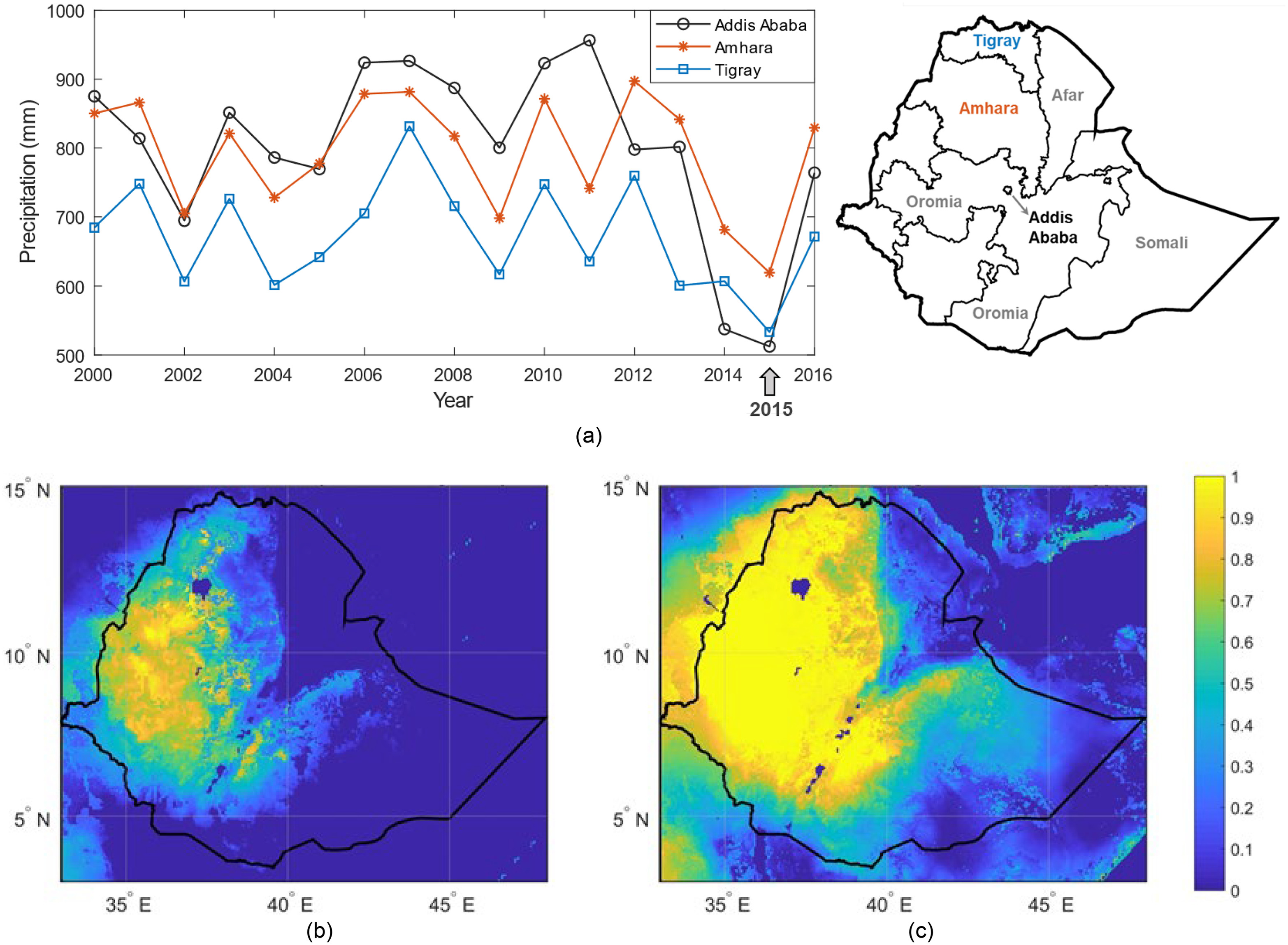
Uneven spatial and temporal distribution of naturally occurring water resources can cause flood and drought, decrease crop production, and increase food insecurity. The effects are exacerbated under climate change, threatening livelihoods in countries that rely heavily on rainfed agriculture. Ethiopia—with less than 3% of irrigated farmland (calculated value for 2015; FAO 2016; World Bank 2019), 41% of GDP dependent on agriculture, and over 70% of labor force with main occupation in agriculture (World Bank 2015, 2017)—is extremely vulnerable to the changing climate. In 2020, for instance, climate shocks such as erratic rainfall, pest infestations, and ethnic conflict are projected to increase emergency needs for food and displaced populations, leading USAID to estimate that at least 8 million people will require humanitarian assistance (USAID 2020). Rainfall variability in Ethiopia is also highly heterogeneous. For instance, while the communities were still in recovery from a severe drought in 2016, which impacted the north and central highland regions in Ethiopia, the subsequent 2017 drought led to extensive crop failure and livestock losses in the south (USAID 2022). Going forward, climate variability will continue to be a major contributing factor in Ethiopia’s food security challenges (USAID 2015), while climate change projections show great uncertainties in the direction of rainfall change in this region (Trisos et al. 2022).

Ethiopia needs more productive agriculture to strengthen the foundation of its economy, and more urgently, to achieve food security. The government of Ethiopia has actively promoted irrigation as an effective tool to mitigate climate impacts and improve agricultural yields (Ethiopia National Planning Commission 2016). The official performance evaluation of its national Growth and Transformation Plan (GTP), which was implemented over the period of 2009 and 2010 through 2014 and 2015, estimates that 2.34 million hectares (ha) of land is developed through small-scale irrigation schemes during the plan period (Ethiopia National Planning Commission 2016). However, other sources report a much smaller expansion of area equipped for irrigation. For example, according to the AQUASTAT database (FAO 2016), Ethiopia was reported to have 860,000 ha equipped for irrigation in 2015, up from 690,000 ha in 2010. While there is uncertainty regarding the size of historical and existing irrigating area because of variations in data sources, the consensus is that Ethiopia has a great irrigation potential and is in urgent need to reduce its dependence on rainfed agriculture (Ethiopia National Planning Commission 2016; Haile and Kasa 2015; Mendes and Paglietti 2015; Mirzakhail et al. 2012).

The potential of irrigable land ranges from a lower value of 2.7 million ha estimated by FAO (Mendes and Paglietti 2015) to an upper value of 5.1 million ha estimated by the Ethiopian government (Ethiopia National Planning Commission 2016; Mirzakhail et al. 2012). Other literature provides estimates around 3.5 million ha (Awulachew et al. 2007; Hagos et al. 2009; Haile and Kasa 2015). Given that 74% of all farmers in Ethiopia are small-holders, who work on land-holdings of up to approximately two hectares (FAO 2017), small-scale irrigation plays an important role in expanding irrigation nationwide. That is, small-holder farmers can operate and maintain a type of irrigation technology effectively by themselves to supplement unreliable rainfall at small-scale plots.

Groundwater irrigation is well suited for widely dispersed small-holder farming communities because of its flexibility and affordability. In contrast, a stable surface-water irrigation system often requires large-scale public investments and favors clustered farming communities or large-scale farms (Pavelic et al. 2013). A traditional focus on irrigation using surface water in Ethiopia, such as individual household-based river diversions and rainwater harvesting, or a larger-scale community-based irrigation withdrawal from a reservoir, has tended to distract decision makers from the potential of groundwater irrigation (Chokkakula and Giordano 2013). Ethiopia has a vast and nearly unexplored groundwater potential, estimated to be 2.5–47 billion cubic meters (Awulachew et al. 2007; Ethiopia Ministry of Agriculture 2011; Makombe et al. 2011; Mengistu et al. 2021; Mirzakhail et al. 2012). This suggests that a more broadly accessible small-scale irrigation strategy that uses groundwater rather than surface water could be valuable, and its growth may well be spurred by improved access to drilling services and pumps at low costs (Villholth 2013).

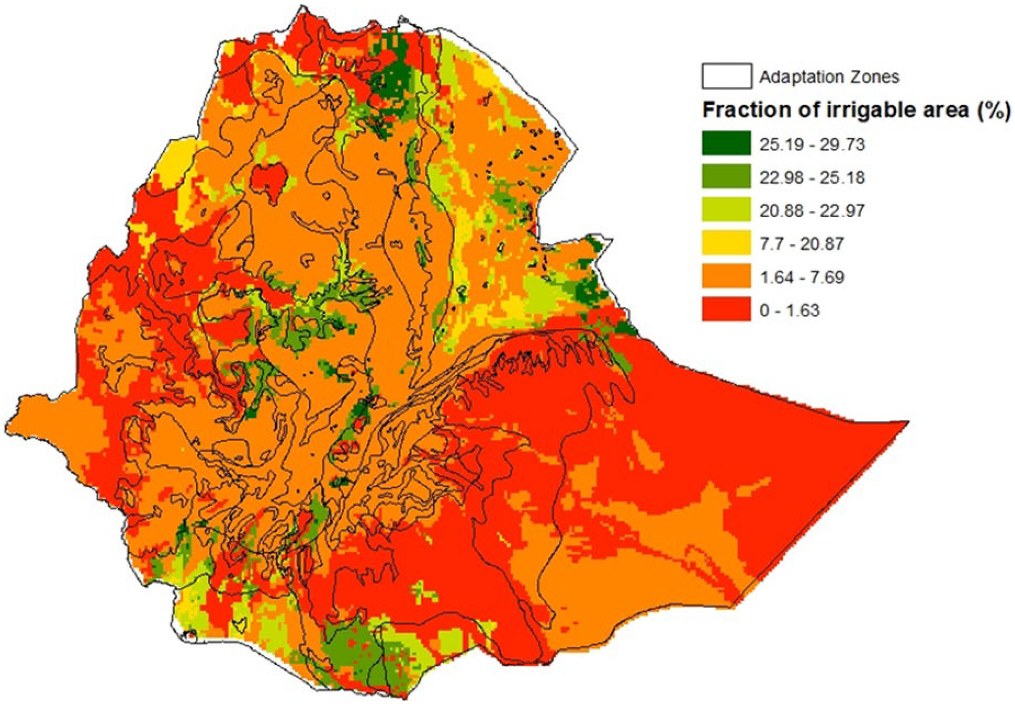
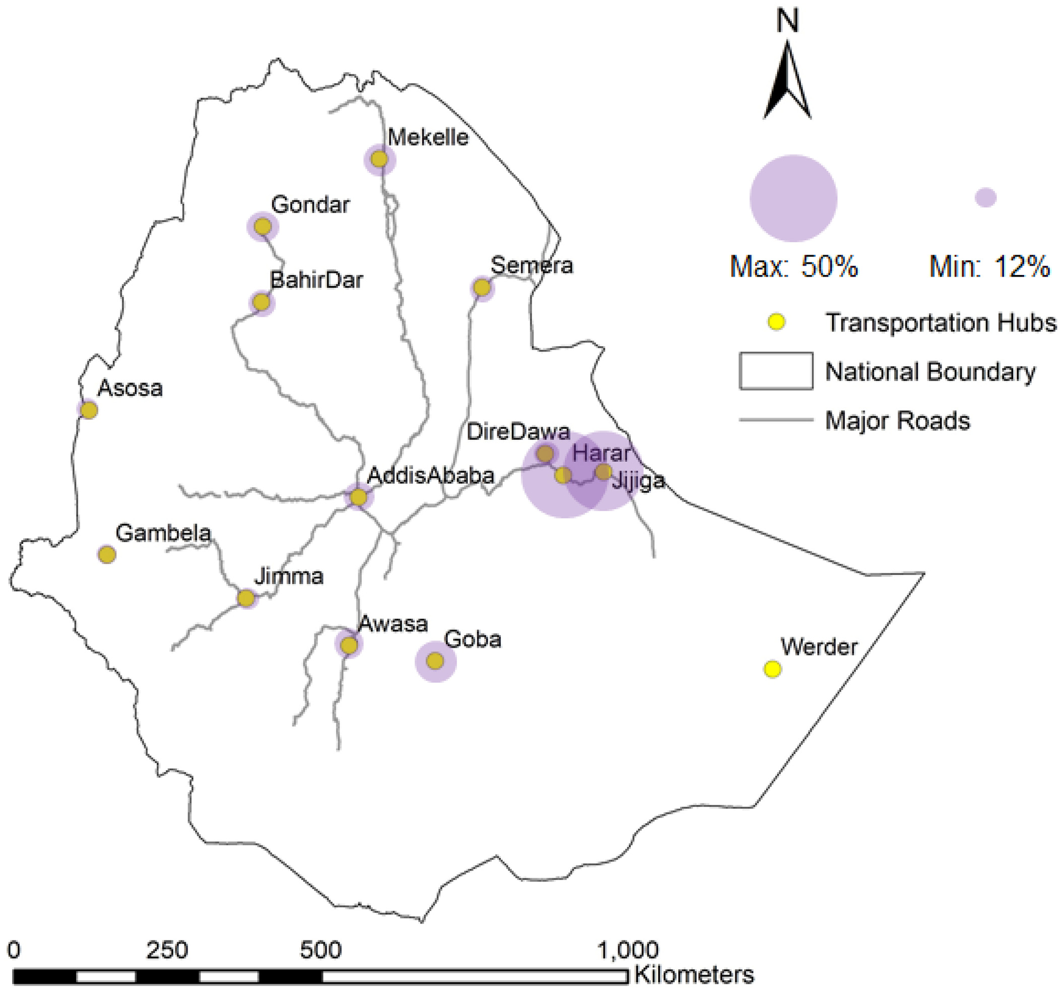
A few studies estimate the groundwater potential for irrigation covering all or a part of Ethiopia (Ayenew et al. 2013; Altchenko and Villholth 2015; Worqlul et al. 2017), among which Worqlul et al. (2017) provides spatially explicit estimates of irrigation potential using shallow groundwater (

< 25 m

) at a gridded scale of

1 km \times 1 km

in Ethiopia. They considered key factors including groundwater depth, potential borehole yield, and net irrigation requirement over the growing season to estimate the fraction of potential irrigable area using shallow groundwater (Fig. 1 in this study), which provides favorable locations for small-scale groundwater irrigation as a supplement to rainfall during the growing season. With additional considerations of land use, soil properties, slope, and market access, a total area of approximately 0.5 million ha is considered to be suitable for groundwater irrigation in Ethiopia (roughly 8% of estimated potential irrigable land; Worqlul et al. 2017).

Fig. 1. Fraction of potential irrigable area using shallow groundwater ( $< 25 m$ ) overlaid with the boundaries of adaptation zones (a spatial unit implemented in this study). (Data from Worqlul et al. 2017.)

Although irrigation may improve crop yield under climate variability and climate change, there is uncertainty in the effect of irrigation on food security because the net benefit can be specific to location and stakeholder. Additionally, irrigation is influenced by different factors, such as allocation of crop land, market access, and crop prices. A sustainable groundwater irrigation plan may also be desirable and therefore requires ex ante evaluation to avoid overexploitation.

There are some studies that develop decision support tool for farmers in agricultural planning and management, including the application of irrigation (e.g., Rader et al. 2009), while only a few studies evaluate irrigation effects on food security, the economy, and the environment through an integrated model framework (e.g., Cai et al. 2003; Clarke et al. 2017; Worqlul et al. 2018; Jander et al. 2023; Gai et al. 2022), and these studies are scaled from farm to basin level and rarely include market access when evaluating the food security and economic outcomes of irrigation. For instance, Clarke et al. (2017) applied an integrated decision support system to investigate the influences of new farming technologies (including irrigation) on production and economic outcomes at two representative farms in Ethiopia while minimizing negative environmental impacts at the watershed scale. Although the two farms were selected to ensure a reasonable access to markets, they did not include an endogenous interconnected food market network in their model beyond the area of the farms.

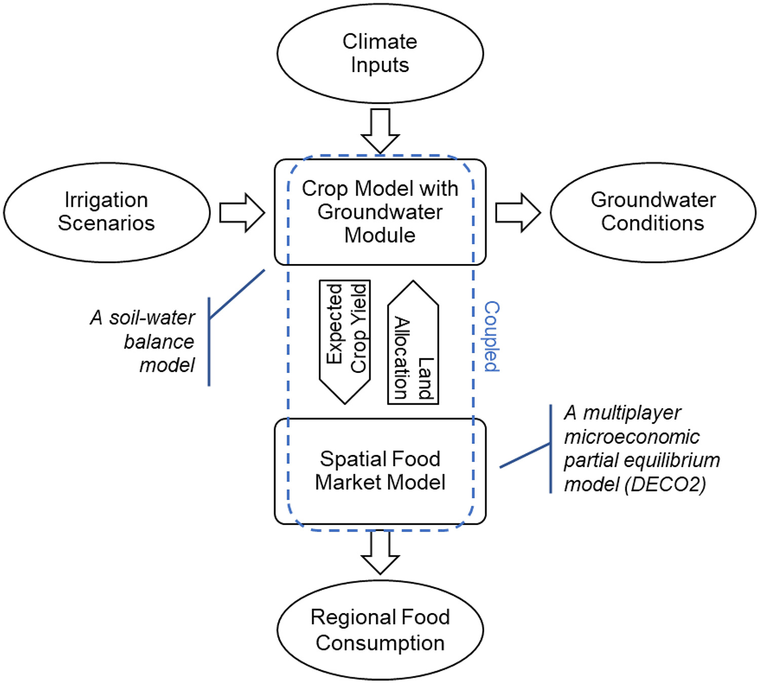
In this study, we develop a new systems modeling tool that can integrate knowledge from hydrology, agriculture, and economics to understand the effect of irrigation on food security and groundwater sustainability. Although individual models exist for these factors, a bottom-up integration of these factors has yet to take place in the context of Ethiopia, a climate-vulnerable country. We address this gap in the literature by developing an integrated model that couples crop yield, subsurface hydrology (including groundwater recharge), and spatial food markets (Fig. 2). Specifically, a gridded process-based crop model across Ethiopia is coupled with a spatially interconnected food market model at the national scale. We use this integrated model for regional evaluation of food security under different small-scale irrigation scenarios, while also endogenously tracking the associated groundwater resources in Ethiopia. We compare two main outcome variables—the resulted regional crop consumption and groundwater storage change—under different irrigation scenarios to evaluate the effect of irrigation. In this way, we test the hypothesis of whether small-scale irrigation can improve food security under changing climate and water resource conditions in the country. It is worth noting that crop produced in one area may not be consumed in the same area because of spatial transport and trade (both domestic and international trade). The spatially interconnected food market model included in this integrated modeling framework can capture the effect of trade on regional crop consumption. Therefore, we also compare other outcome variables, such as transport and export of crops, under different irrigation scenarios to diagnose the underlying mechanism of how irrigation affects food security.

Fig. 2. Coupled model framework. DECO stands for Distributed Extendible Complementarity model.

The following section describes the model in detail and presents the small-scale irrigation scenarios imposed to evaluate the corresponding subnational impacts. Next, we present the model results, followed by a discussion section, where we discuss the broader implications of the study results as well as the limitations of this study. Last, we conclude with the key findings of our study.

Methods

Extended from a previous study (Sankaranarayanan et al. 2020), we develop a coupled model framework, which includes a crop model, a spatial food market model, and a closed feedback loop between them (Fig. 2). The crop model and its coupling to the spatial food market model are new developments since the previous study, where the spatial food market model was developed. The crop model simulates crop yields based on soil properties, crop characteristics, climate conditions and irrigation scenarios. The simulated crop yield is then taken as the input to the food market model, affecting decision-making on crop land allocation, together with other decision factors such as total available land, cost of farming (including cost of switching between crops), and endogenous crop prices. Once their decisions on land allocation are made, this information is taken back to the crop model to compute the associated groundwater conditions. In the spatial market model, farmers’ decisions act on the supply chain of crops through a connected food market network with explicitly modeled road infrastructure for crop transport costs, which results in food consumption at the subnational level.

Crop Model with Groundwater Module

The crop model is a gridded process-based soil-water balance model that takes climate inputs (e.g., temperature and precipitation), irrigation amount, soil water holding capacities, and crop-specific characteristics (e.g., crop calendar and drought resistant extent) as inputs. The model tracks the daily soil moisture change over time, simulates daily crop root growth and evapotranspiration, and produces a ratio of expected crop yield over maximum yield for each growing period [Eq. (1)]. The ratio is called a yield factor. It ranges from 0 to 1 given different climate and irrigation conditions during the growing period. The maximum yield is defined as the yield where there is no water stress for the crop to grow. A yield factor multiplied to the maximum yield gives the actual yield under potential water stress. Therefore, a yield factor of zero indicates crop failure (i.e., zero crop yield), whereas a yield factor of one indicates there is no water stress on the crop yield

Y F_{c} = \frac{Y a_{c}}{Y m_{c}}

(1)

where

Y F

= yield factor;

Y a

= actual yield under potential water stress; and

Y m

= maximum yield for crop

c

over a growing period. The yield factor is estimated using

Y F_{c} = 1 - K y_{c} (1 - \frac{E T_{c a d j}}{E T_{c}})

(2)

where

K y

= empirical yield response factor, which varies across crop types;

E T_{c a d j}

= adjusted (actual) crop evapotranspiration; and

E T_{c}

= crop evapotranspiration for standard conditions (no water stress).

E T_{c}

is calculated using the reference evapotranspiration, which depends on the local weather, multiplied by a crop-specific empirical coefficient.

E T_{c a d j}

is calculated using the soil-water balance model. The general approach follows Food and Agricultural Organization (FAO) published empirical methodology (Doorenbos et al. 1980; Allen et al. 1998), which has been applied in multiple studies to simulate climate impacts to crop yield (Block et al. 2008; Sankaranarayanan et al. 2020; Williams et al. 2020; Zhang et al. 2020; Lala et al. 2021; Bazzana et al. 2022; Lala et al. 2023). However, building on the previous studies, we developed a new groundwater module within the crop model to simulate groundwater conditions over time given climate inputs, crop patterns, and groundwater exploitation for irrigation. The model is calibrated using climate and land surface model outputs customized for the study region.

The newly developed groundwater module (Fig. S1) takes deep percolation (DP) from the soil column above it as the recharge to groundwater storage over time. A positive DP can occur when there is excess water after going through all the layers in the soil column, likely during an intense rainfall and/or irrigation event. When groundwater irrigation occurs, the needed amount of irrigation water is extracted from the groundwater storage. If the irrigation is overapplied, the remaining water would percolate back to the groundwater reservoir. There is also a baseflow out of the groundwater reservoir, which is calibrated so that the long-term average of daily baseflow equals the long-term average of daily DP. This assumes that groundwater storage under natural conditions does not change in a long-term period. We do not consider lateral flow in this simplified groundwater module. At every time step

i

, the groundwater storage

S

is evaluated using

S_{i} = S_{i - 1} + D P_{i} - B_{i} - I_{i}

(3)

where

B

= baseflow and

I

is the irrigation amount applied, at daily time step

i

. An initial groundwater storage is assumed, and the storage change over time is tracked.

D P

should converge to the same value as the groundwater recharge

R g

after calibration. To obtain the value of

R g

, we need to first estimate the value of

R l

[Eq. (4)], which is then partitioned into the groundwater recharge

R g

and the surface runoff

R s

[Eq. (5)]

R l = P e {(\frac{S S}{S S m a x})}^{γ}

(4)

where

S S

= soil water content and

S S m a x

is the total available soil water capacity, within the effective root zone;

γ

= calibration parameter called the runoff coefficient; and

P e

= effective precipitation [Eq. (6)]. The calculation of

R l

follows the approach of Bergström (1995), which is applied in the WaterGap Global Hydrology Model (WGHM; Döll et al. 2003). We calibrate

γ

and the partition of

R l

into surface runoff

R s

and groundwater recharge

R g

, such that

D P

and

R g

converge to the same value after model calibration

R l = R g + R s

(5)

where

R l

= lumped sum of groundwater recharge

R g

and surface runoff

R s

. This approach is also applied in the WaterGAP model (Döll et al. 2003; Döll and Fiedler 2008; Hunger and Döll 2008).

The calibration is performed using simulation outputs from the Noah Multiparameterization Land Surface Model (Noah-MP LSM, version 3.6; Niu et al. 2011) within the framework of NASA’s Land Information System (LIS; Kumar et al. 2006). Building on its earlier versions of Noah LSM (Ek et al. 2003), Noah-MP offers multiphysics options such as dynamic leaf, groundwater, and runoff schemes, and has delivered robust performance in the simulation of water and energy fluxes in many river basins across the globe (Yang et al. 2011; Cai et al. 2014). Noah-MP LSM simulations used the Moderate Resolution Imaging Spectroradiometer-International Geosphere Biosphere Program (MODIS-IGBP; Friedl et al. 2010) 1-km resolution land cover, State Soil Geographic (Schwarz and Alexander 1995) 1-km resolution soil texture, and 30-m resolution Shuttle Radar Topography Mission elevation data (Farr et al. 2007). The simulation is forced by the combination of two atmospheric forcing data sets: NASA’s Modern Era Reanalysis for Research and Applications version 2 (MERRA-2; Bosilovich 2015) and the Climate Hazards group Infrared Precipitation with Stations data (CHIRPS; Funk et al. 2015). CHIRPS has been temporally disaggregated from daily to 6-hourly at 0.05° spatial resolution providing rainfall input to Noah-MP while MERRA-2 provides the remaining meteorological inputs such as temperature, humidity, radiation, and wind at hourly scale. The simulation was run at a spatial resolution of 5 km and the outputs of surface and subsurface runoff, groundwater recharge, and soil moisture change for the period of 2000–2015 are used for calibration analysis. Additional information on the calibration can be found in the Supplemental Materials.

To calculate effective precipitation, we incorporate a new equation for canopy interception [Eq. (6)] in the crop model. Note that the total rainfall would be partly intercepted by plant canopy and the remaining part (i.e., the throughfall) either becomes surface runoff or infiltrates the soil column. Compared to the original model structure (Sankaranarayanan et al. 2020), which implicitly assumes a certain portion of the total rainfall does not reach the soil, our updated approach takes account of the effects of canopy interception and loss to runoff. Incorporating the canopy interception reduces the total water reaching the soil because of canopy evaporation and increases infiltration to runoff ratio by spreading the rain event out over a longer period of time as throughfall. Meanwhile, capturing the surface runoff using a well-established analytical equation (Döll et al. 2003) enables us to better calibrate the crop model against data from land surface model simulations and create a computationally efficient crop model in the two-way coupling model framework (i.e., with the spatial food market model).

Specifically, the canopy interception [Eq. (6)] is estimated using the monthly Greenness Vegetation Fraction (GVF) map over 2002–2015, which is derived from Moderate Resolution Imaging Spectroradiometer’s Normalized Difference Vegetation Index (MODIS NDVI; Huete et al. 1999) data using methods described in Case et al. (2014) as implemented by Nie et al. (2018). This data set provides vegetation greenness information in the range of 0 to 1 at the global gridded scale. In land surface models, GVF is widely used to calculate the canopy interception (Kumar et al. 2018). In order to obtain the GVF or canopy interception ratio for main crop types (e.g., maize, millet, teff, wheat, sorghum, and barley) such that we can model the climate and irrigation effects on crop yield specifically for each crop type, we overlay the monthly GVF map averaged over the available years with the livelihood zonal map in Ethiopia, which identifies where main crop types are grown (FEWS NET 2018). Subsequently, we estimate the canopy interception ratios for each crop type over each growing stage (i.e., planting, vegetative, flowering, yield formation, and ripening, spanning different months) using the spatial average value of GVF in areas where each main crop is growing

P e = (1 - G V F) \times P

(6)

where

P e

= effective precipitation or throughfall given the total precipitation

P

and the

G V F

.

Spatial Food Market Model

The improved Distributed Extendible COmplementarity model (DECO2; Sankaranarayanan et al. 2020) is a multiplayer microeconomic partial equilibrium model, which is designed and calibrated to simulate the responses of Ethiopia’s food markets under potential external shocks. In the model, there are multiple representative players or market actors along the food supply chain, including crop producers, distributors, storage managers, and consumers across subnational zones (Fig. S2). The crop producers sell crops to distributors. The distributors transport the crops across zones and sell them to storage managers, who then sell them to consumers. The model solves for equilibrium between supply and demand for every exchange between two representative players, while every representative player maximizes her own profit or utility noncooperatively. This is framed as a mixed complementarity problem and thus the so-called “COmplementarity” model. While partial-equilibrium models are common for analyzing food markets (e.g., FAO 1998; Rosegrant et al. 2008; Wailes and Chavez 2011; Robinson et al. 2015), DECO2 and its original DECO (Bakker et al. 2018) distinguish themselves by providing a detailed modeling of market actors across the country and their decision-making process, and by serving as a tool for subnational analyses of trade and commerce in Ethiopia. Mathematical formulations of DECO2 are provided in the Supplemental Materials.

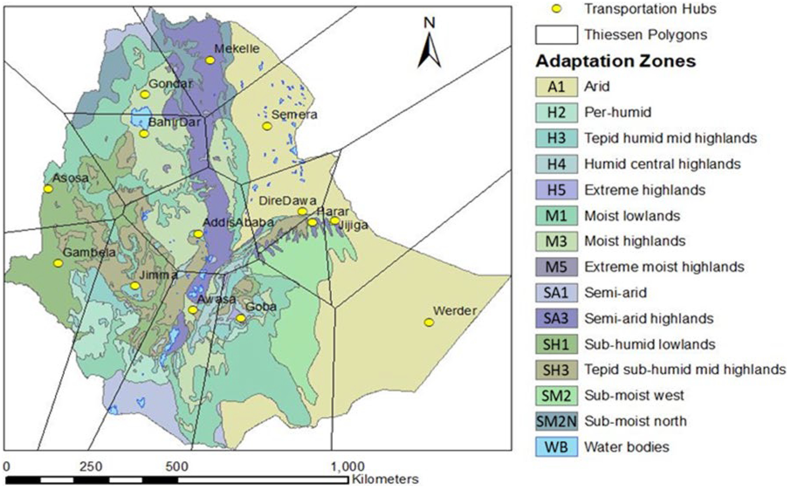
The model is also spatially disaggregated with representative players in each subnational zone or food market. There are two different layers of spatial disaggregation in the model. The first layer is based on adaptation zones (Fig. 3), which are defined by Ethiopian government considering agroclimatic factors (Federal Democratic Republic of Ethiopia 2015). With one representative crop producer in each zone, application of the adaptation zones allows us to better represent production activities integrated with climate and soil characteristics within each zone. However, using adaptation zones to model crop transport with one representative distributor in each zone is inappropriate, because some adaptation zones spread far distances and some are noncontiguous. Therefore, the second layer of spatial disaggregation is based on selected transportation hubs in cities with the actual road network connecting them to endogenously model crop transport in the country (Fig. 3). We then apply Thiessen polygons (Thiessen 1911) surrounding the transportation hubs to connect the two different layers (Fig. 3). A Thiessen polygon has the property that every point in that polygon is the closest to the center (i.e., the transportation hub) within that polygon. We assume that the representative crop producer in any adaptation zone sells in one or more markets proportionally based on the overlap between the adaptation zone and each market’s Thiessen polygon. This indicates that the crop productions are sold to the closest markets geographically.

Fig. 3. Spatial disaggregation of Distributed Extendible COmplementarity model (DECO2) with two different model spatial units of adaptation zones and Thiessen polygons centered around transportation hubs (i.e., food markets). [Reprinted with minor modifications from Sankaranarayanan et al. (2020), under Creative Commons-BY-4.0 license (https://creativecommons.org/licenses/by/4.0/).]

In each adaptation zone, the crop producer decides the land allotted to each crop with the objective of maximizing her profit. We model individual primary food crops, which include teff, sorghum, barley, maize, and wheat, a representative secondary food crop of vegetables, and a lumped cash crop of coffee and oil seeds. The crop producer makes decisions based on the expected yield of each crop, the producer price (i.e., the price the crop producer sells to the distributor), and the costs of production including a penalty term for switching crop types in the same farmland over growing seasons.

The distributor at a transportation hub then distributes the collected crop production from multiple adaptation zones to the spatially connected transportation hubs (i.e., food markets). The flow-in (flow-out) of crops at each transportation hub is balanced out with the supply deficit (surplus) at this hub. That is, the distributor transports crops from high supply and low demand areas to low supply and high demand areas, bearing the transportation costs, while making profits from the differentiated local market prices. All the crop prices including the producer and the consumer price are endogenously solved at each food market. In addition to the transportation hubs, an external node for international import and export is connected to the transportation hub in the capital city (i.e., Addis Ababa). International import (export) occurs only when the domestic crop price at Addis Ababa is higher (lower) than the sum of global price and the import (export) cost, which are defined exogenously.

DECO2 can be solved at yearly time-steps, with two growing seasons per year. The model solves three years altogether and only keeps the first year’s output in a rolling horizon. In this way, the players neither have perfect knowledge of the future, nor are they short-sighted. DECO2 is calibrated against historical data, including crop area and production at the administrative zonal level mainly in the cropping year of 2015 (Central Statistical Agency of Ethiopia 2015). The two growing seasons in Ethiopia are “meher” and “belg.” “Meher” is the main growing season, which produces over 70% of all food (Sankaranarayanan et al. 2020) and relies on the rains falling primarily on western Ethiopia during June–September (Zhang et al. 2016). The latter relies on the minor rainy season spanning March–April. On the consumption end, we assume that all produced crops are consumed. The quantity demanded is proportional to the population in each transportation hub and the area surrounding it (i.e., the Thiessen polygon). We then obtain price elasticity of demand from Tafere et al. (2010) to derive the food demand curves for food markets in Ethiopia. Given the supply of food and demand of food, we synthetically generate the food transport quantities in the model. Subsequently, the model calibration is achieved by appropriately adjusting the input parameters, namely the crop production costs and the slope and intercept of the demand curves. We refer the reader to Sankaranarayanan et al. (2020) for more information on the model.

Model Coupling

The crop model and the spatial food market model are coupled through the feedback of expected yield and allotted land of different crops. This way of coupling the model assumes that the farmers have reasonably a good understanding of their crops’ yield with respect to water availability. Specifically in the coupled model, the baseline yield can be calculated given the historical crop production divided by the corresponding crop area. Using the baseline (actual) yield in combination with the yield factor in the same year, which is calculated by the crop model, we obtain the maximum yield for each crop type. The maximum yield multiplied by an alternative yield factor under a different water condition leads to a different crop yield from the baseline. With this coupled model, we can study the effects of irrigation on crop yield and the subsequent responses in crop production, transport, and consumption at spatially disaggregated levels.

As we feed the expected crop yields from the crop model into DECO2 to drive crop producers’ decision-making, the resultant crop land allocations are fed back into the crop model to estimate the effect on groundwater conditions. The crop patterns in each adaptation zone affect the groundwater conditions through crop-specific canopy interceptions and crop water requirement (i.e., evapotranspiration). In addition, spatially varying soil properties (e.g., water holding capacity) and crop-specific calendars in combination with the spatial-temporal climate conditions (e.g., daily precipitation and temperature at a gridded scale) also affect the groundwater conditions. If groundwater irrigation exists, in addition to the direct impact on groundwater conditions through water withdrawals, the indirect impact through the change of crop patterns in each adaptation zone is also accounted for.

The crop model operates at a gridded scale that covers Ethiopia and produces an estimated yield factor in each grid-cell as if a certain type of crop is grown at this grid-cell. The gridded yield factors are then aggregated to the level of the adaptation zone using area-weighted averages, which are then taken into consideration by the representative crop producer in each adaptation zone to maximize her own profit in DECO2. The associated effect on groundwater conditions in each adaptation zone is calculated using the ratio of crop area (from DECO2) over total land area in this zone multiplied by the sum of groundwater storage change over all the grids in this zone. More details on the model coupling can be found in the Supplemental Materials.

Irrigation Scenarios

To show the coupled model’s capability, we run a scenario where an irrigation of

2 mm / day

is available to maize in every adaptation zone. Maize is one of the primary food crops in the country, ranking first and second in production and farming area, respectively (Central Statistical Agency of Ethiopia 2015). Maize is also more sensitive to dry conditions than the other primary food crops (Zhang et al. 2020). Under the irrigation scenario,

2 mm / day

acts as supplementary irrigation to maize during the main growing season (i.e., “Meher”). In comparison, the calibrated baseline in 2015 is treated as no irrigation available for any of the crops. This is a reasonable assumption given Ethiopia’s small irrigation extent in 2015. The fraction of irrigable area using shallow groundwater (

< 25 m

) in each adaptation zone (Fig. 1) is also considered as an upper limit when we implement the irrigation scenario. That is, the total area being irrigated cannot exceed the irrigable area using shallow groundwater defined based on Worqlul et al. (2017). By comparing the irrigation scenario to the baseline, we address the “what-if” question in the base year of 2015, a year of significant drought and crop failure over a large portion of Ethiopia (Singh et al. 2016). That is, whether small-scale irrigation using groundwater can improve food security under the changing climate and water resource conditions in Ethiopia. We do not consider irrigation cost in this study.

While our study assumes that the irrigation is only available to Maize, it is of course realistic to expect that crop producers might use the irrigation for other crops too. Cash crops such as fruits and vegetables may be more likely to be irrigated than maize; however, the current crop yield model is only capable of modeling the primary food crops (i.e., maize, millet, teff, wheat, sorghum, and barley). Because of this model limitation as well as the nature of maize and its prevalence in Ethiopia compared to other primary food crops, most of the irrigation water is likely to be used by maize. We encourage readers to understand this scenario as one of small-scale irrigation possibilities, rather than an exact representation of what will happen, and interpret the associated results with this scenario setup in mind. The goal here is not to come up with the exact mix of crops that will be irrigated in this scenario, but the impact on groundwater from a resulting mix of crops after irrigation schemes have been applied.

Results

Spatial Effects of Irrigation on Cropland Allocation and Production

We observe that the yield of maize improves given the available groundwater irrigation compared to the nonirrigated baseline. However, the extent of improvement varies across space with significant positive effects observed in fertile and temperate, but drought-prone areas. The improvement is attributed to the increase in crop yield under irrigation, rather than an extensification of the cropland.

In 2015, the northwestern part of the country was dry during the main rainy season (June–September) with considerably less rain than historical average [Fig. 4(a)]. As a result, simulated maize yield in those regions is stressed by insufficient water in the baseline without irrigation, where the estimated yield factors for maize are less than one for most areas [Fig. 4(b)]. Under the irrigation scenario, there is an overall increase of maize yield factors, particularly in places where soil is fertile and temperature is moderate, such as northwestern Ethiopia [Fig. 4(c)]. In contrast, some regions still have low yield factors under the irrigation scenario because of low soil fertility and immoderate temperature, including the Somali and Afar regions (Fig. 4), which are mostly desert. This is also consistent with the map of adaptation zones, where the “arid” category (i.e., A1) overlaps a large part of Somali and Afar (Fig. 3).

Fig. 4. (a) Total precipitation during Ethiopia’s main raining season (June–September) from 2000 to 2016 in Addis Ababa, Amhara region, and Tigray region; (b) the calculated yield factor for maize in 2015 without irrigation; and (c) with irrigation of targeted $2 mm / day$ . The yield factor ranges from 0 to 1, where 0 means crop failure and 1 means no water stress. A map showing administrative regions mentioned in the text is provided in (a).

In the baseline, the largest farming area among adaptation zones is located at the moist highlands [i.e., M3; Fig. 5(a)], most of which overlaps with Amhara and Oromia region in the northwest and was significantly impacted by the dry conditions in 2015. Overall, about 30% of M3’s land is used to grow crops, indicating relatively high fertile soil in this zone particularly compared to the arid zone (i.e., A1) where 0% of its land is used to grow crops [Fig. 5(a)]. A relatively large farming area of maize is found in the tepid subhumid mid highlands (i.e., SH3) and the moist highlands (i.e., M3), compared to other adaptation zones in Ethiopia [Fig. 5(a)].

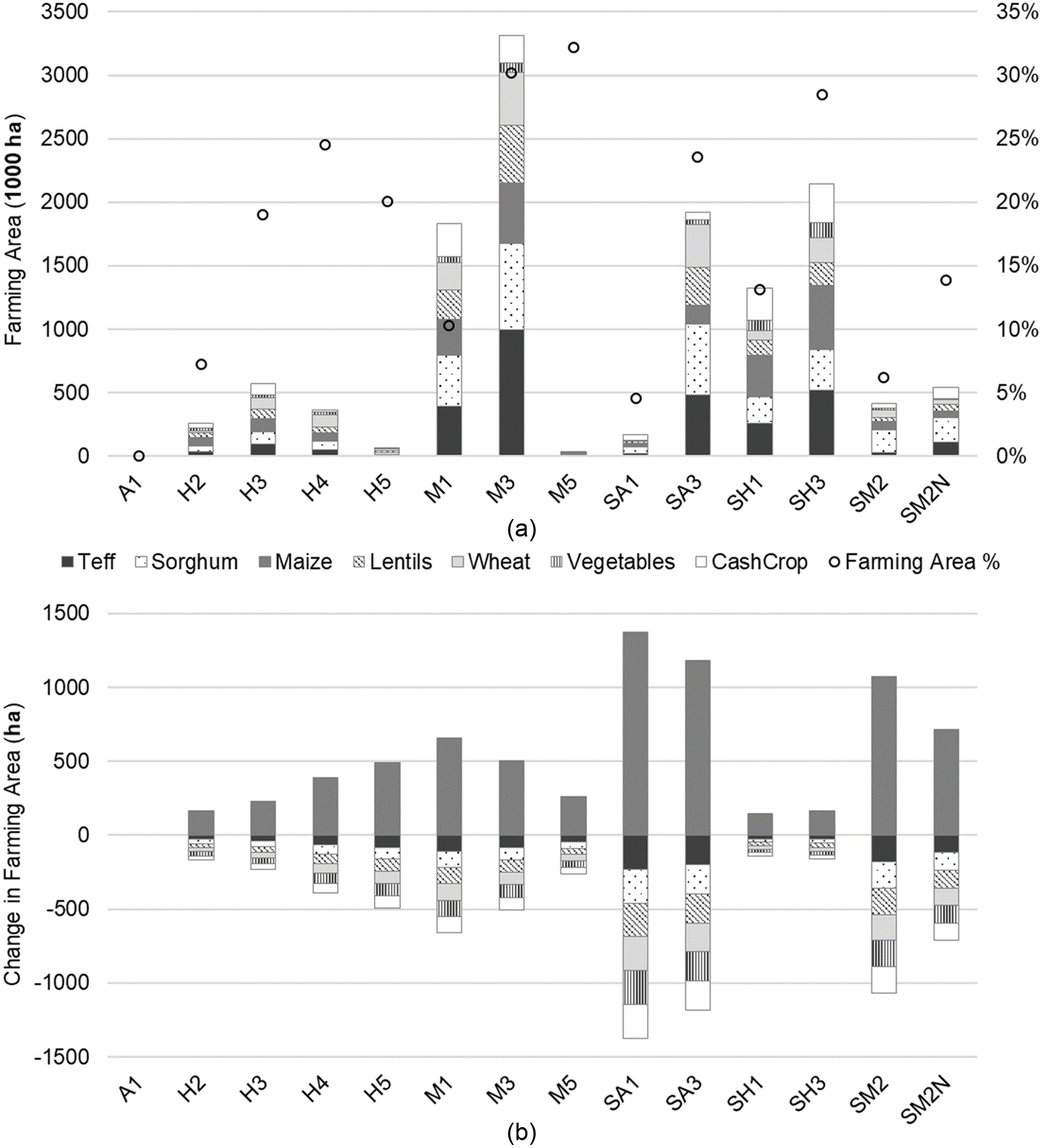
Fig. 5. (a) Farming area allotted to each crop in each adaptation zone shown with stacked bars at the baseline (without irrigation); and (b) the changes in farming area by crop under the irrigation scenario compared to the baseline, where the positive changes are for maize only while negative changes are stacked together for other crops. The positive change in farming area in each adaptation zone is similar to the aggregate negative change, and thus the total farming area for all the crops is barely changed. The percentage of total farming area of the total zonal area is shown using circles in (a) with a secondary y-axis on the right. Note that the y-axis of the farming area in (a) is on a different scale from the y-axis in (b).

The largest changes in cropping patterns under the irrigation scenario compared to the baseline occur in the semiarid zones, SA1 and SA3 [Fig. 5(b)], where without irrigation growing maize can be difficult and nonprofitable. Therefore, under the irrigation scenario, crop producers in the two zones switch relatively large farming areas to grow maize. However, the switched farming area is a very small portion of the total farmland for all adaptation zones (

< 0.1 %

overall; Fig. 5). Therefore, the crop patterns alter only slightly under the irrigation scenario. Additionally, the total farming area for all the crops is barely changed, as the model heavily penalizes changes of the farming area. The penalty is applied to represent the land tenure system in Ethiopia, which limits rural households’ farmland access.

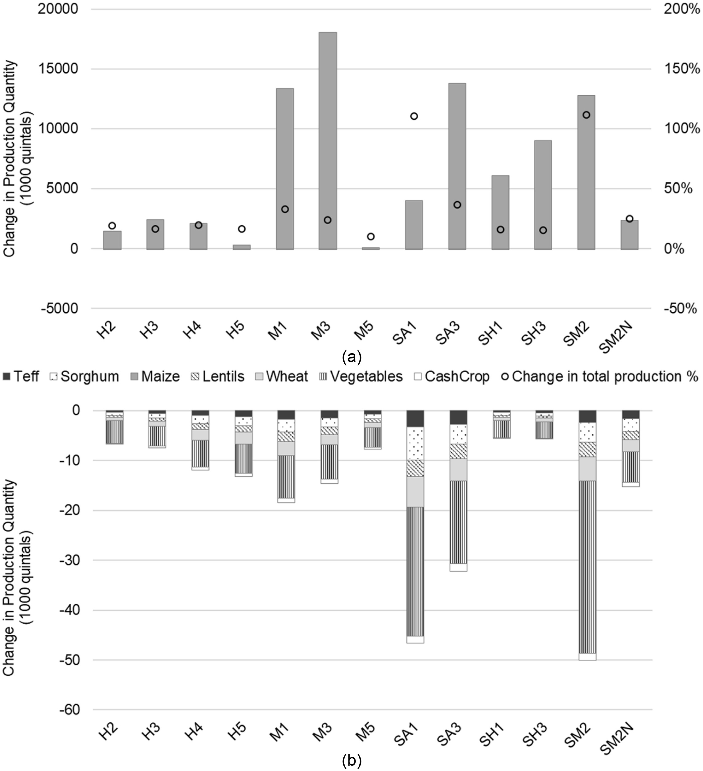
Although the total farming area barely changes under the irrigation scenario, the total production of all crops increases more than 100% in some adaptation zones (Fig. 6). This is because the production of maize increases sharply under the irrigation scenario despite the slight decrease in the production of all other crops. It indicates that the yield of maize per unit of land is increased because of the availability of irrigation to maize. The crop producers are willing to allot more land to grow maize instead of the crops that are planted in the baseline, resulting in a reduced production of all other crops except maize. Among the adaptation zones, the moist lowlands and highlands (i.e., M1 and M3), which were heavily hit by the 2015 drought, benefit the most from the irrigation with the largest increase in total production under the irrigation scenario compared to the baseline.

Fig. 6. Changes in production quantity for (a) maize (positive change) and all other crops in the model (stacked bar of negative changes) in each adaptation zone under the irrigation scenario compared to the baseline (without irrigation). The percent change in total production of all crops is also shown using circles with a secondary y-axis on the right. Note that the negative changes for other crops are much smaller than the positive changes for maize and thus are almost invisible in (a). Therefore, (b) shows a zoom in for the other crops (excluding maize).

Associated Effects on the Crop Transport, Trade, and Consumption

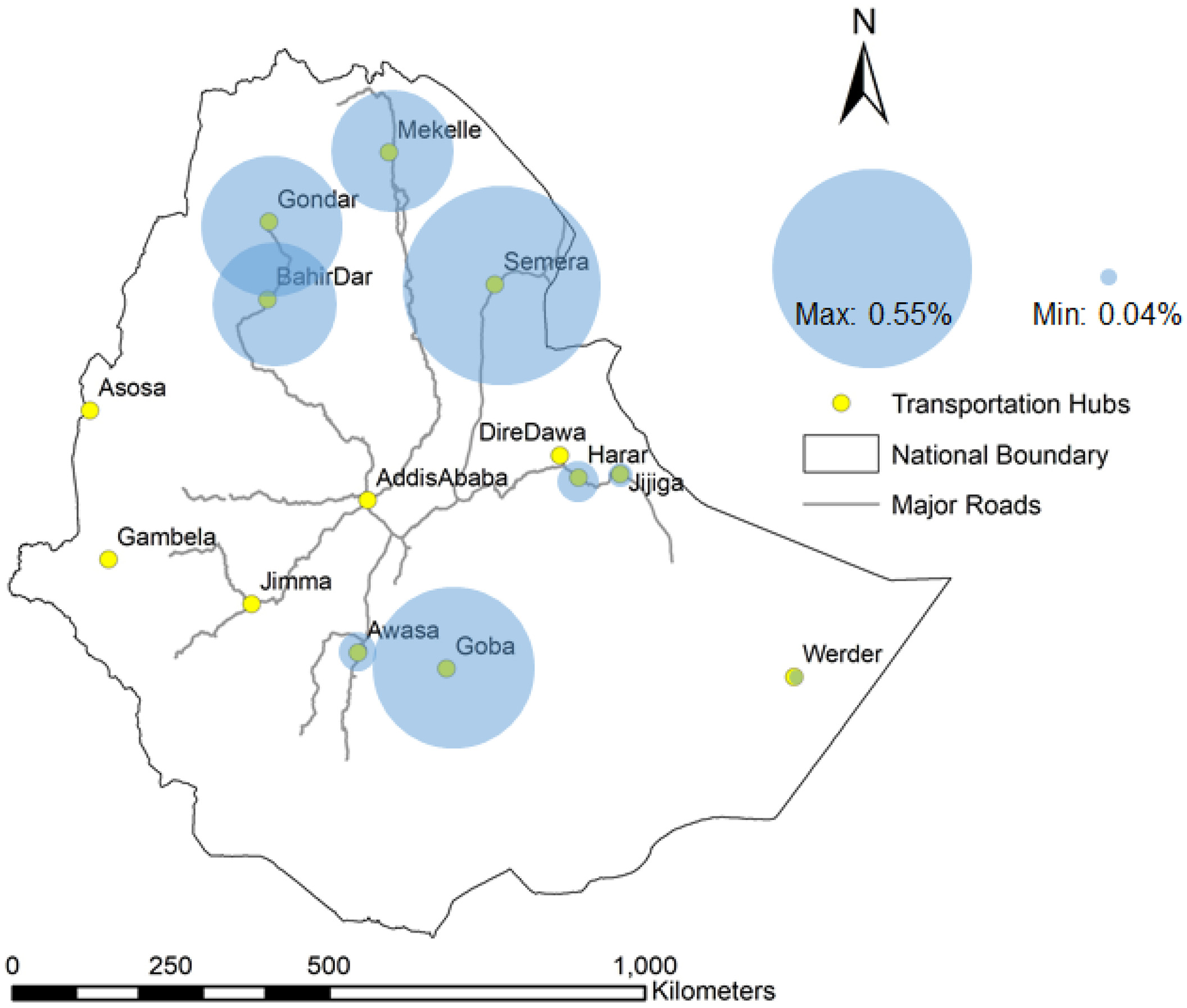
The spatial change of maize production affects the transport of maize for domestic consumption and international export (Fig. 7). The interconnected spatial transport network and the potential for international export lead to only an average of 0.18% increase in domestic food consumption (roughly 0.3 kg per capita) despite a substantial 28% boost in crop production (Fig. 8). This is because distributors are likely to transport the crops for international export because of higher profit than selling them to domestic consumers. As a result, the domestic consumption does not always linearly increase with the production in a region because of the interconnected spatial transport network and the possibility of international export.

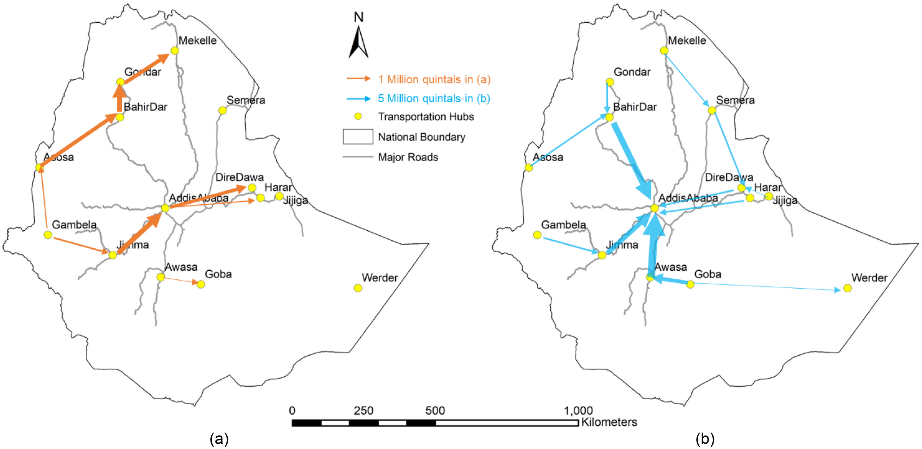
Fig. 7. Maize transport pattern (a) under baseline (without irrigation); and (b) under the irrigation scenario. Note that the arrow scale is changed with the same size arrow under the irrigation scenario representing transporting a quantity 5 times the baseline. A larger quantity of maize is transported to Addis Ababa for international export under the irrigation scenario.

Fig. 8. Percent changes in food consumption (of all crops in quintals) in transportation hubs (i.e., food markets) under the irrigation scenario compared to the baseline (without irrigation).

In general, there is a trend of transporting maize from the west to the east of the country in the baseline; that is, from the more fertile and productive west to the eastern desert. The patterns are changed under the irrigation scenario, where 54% of total maize production is transported to the national capital, Addis Ababa, for international export. For comparison, the international export of maize counts for only 2% of the total maize production in the baseline. This indicates that under the irrigation scenario, distributors are willing to transport the excess of domestic maize supply to Addis Ababa for international export, gaining the profit from the price gap between the domestic and international market. Additionally, almost all food markets become net exporters of maize under the irrigation scenario, indicating a surplus of maize supply compared to demand in most regions.

Associated Effects on Stakeholders’ Profits

The percent change of farmer’s profit increases 18% on average (Fig. 9). The increase is more evident in places where without irrigation maize yield is low. Therefore, irrigation could bring them comparatively high profit. For example, crop producer’s profit in Harar, a food market in the east side of the country, increases 50% under the irrigation scenario compared to the baseline (Fig. 9). Most of the producer sales (to distributer) in Harar is from the submoist west (i.e., SM2), where the irrigation scenario brings over 100% increase in maize production [Fig. 6(a)].

Fig. 9. Percent changes in crop producer’s profit in transportation hubs (i.e., food markets) under the irrigation scenario compared to the baseline (without irrigation).

Associated Effects on Groundwater Storage

The changes in groundwater storage because of the assumed irrigation are comparable to the changes in groundwater storage caused by the drought in 2015 (Fig. 10). Although 2015 is a drought year for a large part of the country, particularly in the moist lowlands, moist highlands, and extreme moist highlands (i.e., M1, M3, and M5), the overall groundwater storage is increased because of an opposite climate effect to other parts of the country. Under the irrigation scenario, groundwater storage decreases in all zones, and the impact of irrigation is generally larger than the negative impact of the drought. As a result, a

2 mm / day

of irrigation for maize causes an average of 4 mm annual reduction of groundwater storage.

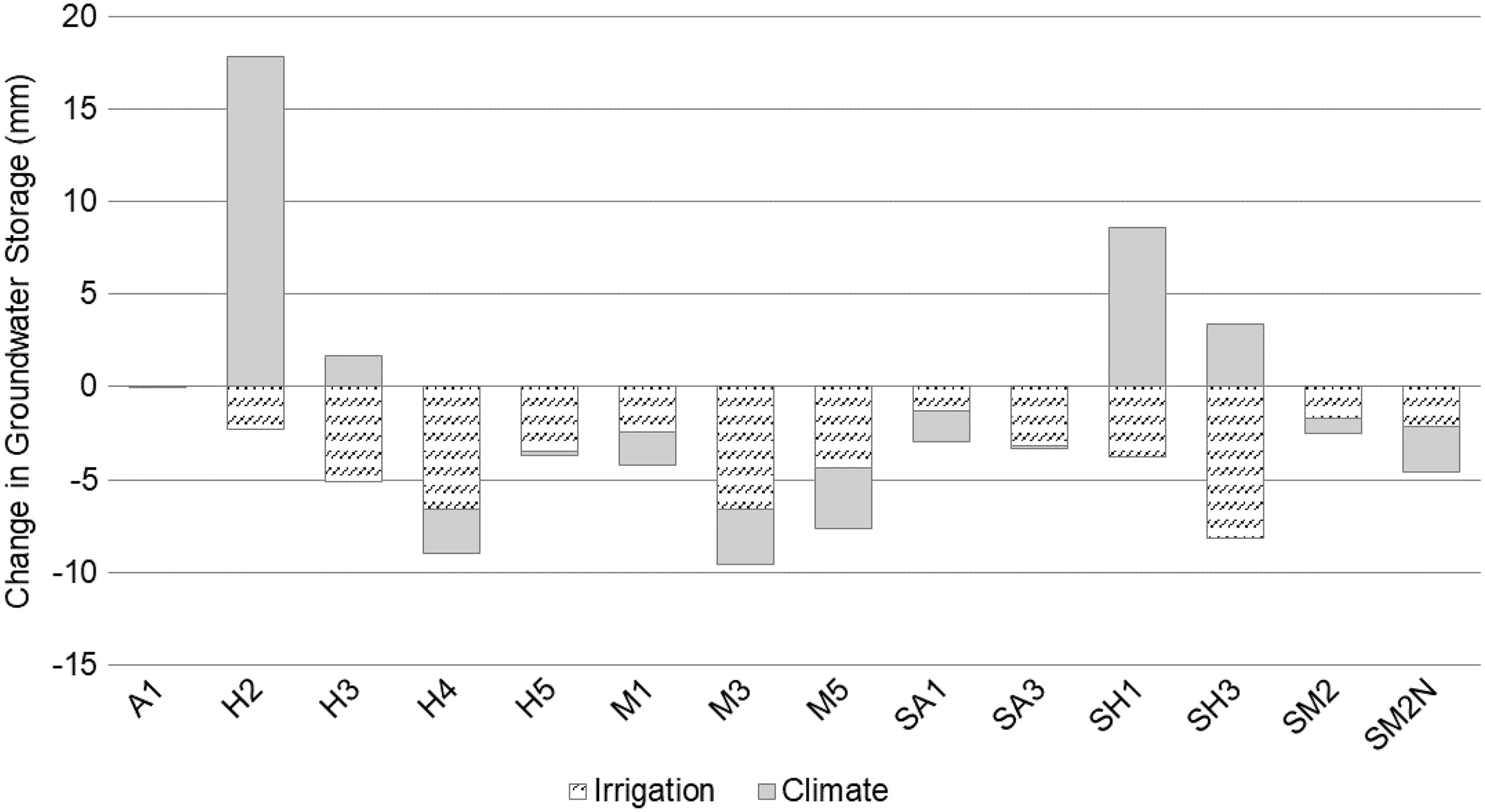
Fig. 10. Changes in groundwater storage due to climate variability (i.e., climate conditions in 2015) and irrigation.

Correspondingly, the annual cumulative change in groundwater storage volume because of irrigation reaches approximately 3 billion cubic meters. Compared to the range of potential groundwater storage reported in the literature (i.e., 2.5–47 billion cubic meters in Ethiopia), the experimental scenario of groundwater irrigation applied to all maize planting areas could potentially deplete the aquifer storage. However, there is a wide range of uncertainty in groundwater storage in the country, and the resultant groundwater storage change because of the assumed irrigation falls at the lower end of the available groundwater storage spectrum. Additionally, the concurrent climate conditions in the model year of 2015 increased the overall groundwater storage by approximately 0.9 billion cubic meters, resulting in a net reduction of 2.1 billion cubic meters in the groundwater storage under the combined effects of climate and irrigation.

Discussion

Despite spatial variability, the overall crop production increases 28% under the irrigation scenario. This result can be contrasted with the simulated economic impact of policies that directly target export policy. For example, following the international food price spikes of 2008, Ethiopia banned the export of teff, a grain that is a primary staple of Ethiopian diets, in order to stabilize the domestic price at a low level and ensure domestic teff consumption. In a previous study (Sankaranarayanan et al. 2020), the authors applied DECO2 to evaluate the effect of lifting the teff ban on the food system in Ethiopia. It was found that the percent change in profit of the crop producer is very small. Even with a free export market where the teff ban is completely lifted, the overall increase in crop producers’ profit is slightly over 0.2%, because the profit from the export is enjoyed almost exclusively by the distributor and storage manager as opposed to the initial production activity. The extra profit cannot pass down to the crop producers because of the lack of market power, transportation infrastructure, and therefore access to multiple markets for the crop producers to sell their teff at a higher price (Sankaranarayanan et al. 2020). In comparison, this study shows that small-scale irrigation, as opposed to lifting the export ban, benefits the crop producer to a much higher extent with crop producers gaining an average of 18% in profits. As an irrigation policy is directly related to the initial production activity, it brings direct benefit to the crop producers. In contrast, lifting an export ban, although increases the demand for crops, does not necessarily benefit the rural crop producers because of poor distribution markets and transportation infrastructure in Ethiopia.

It should be noted that this 28% increase in crop production and 18% increase in producer profits came with only a corresponding 0.18% increase in domestic consumption, because the majority of the increase in production flows to the international export market. This is consistent with what has been found in a previous study, where significant increases in exports of agricultural products were observed given simulated irrigation investments in Ethiopia (Beyene and Engida 2016). Similarly, in another previous study that focuses on the Sub-Saharan African region, it was found that irrigation expansion can shift the region from a net import position to a net export position (Xie et al. 2018). This is also consistent with our finding that the feasibility of irrigation expansion for improving food security not only depends on biophysical factors but also on socioeconomic factors. Considering the importance of food security in Ethiopia, which faces significant food shortage challenges (Abduselam Abdulahi 2017), policymakers may implement relevant policies to increase domestic consumption, such as another restrictive cap on international exports, or a consumer subsidy using export revenue. For example, the Productive Safety Net Program launched by the Ethiopian government has been providing payments to food insecure households to assure food consumption (International Food Policy Research Institute & Ethiopia Development Research Institute 2014). These kinds of policies would shift the balance of irrigation benefits from increased producer and distributor income through trade to increased food consumption—an outcome that might be particularly valuable during drought years like 2015.

The outcome of crop yield and production under the irrigation scenario shows that groundwater is a good buffer of drought during an acute, severe event like the drought of 2015, providing water for the crops when necessary through groundwater irrigation. However, the impact of irrigation on groundwater conditions in the longer term cannot be ignored. Depending on local climate conditions, the reduction of groundwater storage because of irrigation may not be replenished in time during the noncropping season and over the long run, and thus it can lead to gradual groundwater depletion. A set of user-defined irrigation scenarios can be run using our model to evaluate the corresponding groundwater table change along with food security and profits outcomes. Our model can provide insights in developing a sustainable irrigation strategy for the policy-makers.

There are limitations of our model that should be considered when interpreting results. First, we do not model potential traffic congestion. In our model, the travel time is not affected by the level of occupied road capacity, and thus food transport costs, which are a function of the travel time, are not affected. With a greater traffic load toward Addis Ababa for international export under the irrigation scenario, we may be overestimating the quantity of crop transported to Addis Ababa for international export given the possible omitted increase in transport cost. From a policy implementation perspective, the road network expansion may be necessary to facilitate food transport given increased domestic production.

Second, we do not explicitly model the international market for crops. We assume that the changes in Ethiopia’s export would not affect the global market condition. With increase in maize supply in the global market due to Ethiopia’s increasing export of maize under the irrigation scenario, the international price of maize may drop, resulting in a decrease in export profits. Therefore, our results may overestimate the maize export quantity and profit. Future research may improve this part of the model through coupling with a global market model or incorporating a global supply and demand curve.

Third, the groundwater module does not simulate lateral fluxes of groundwater; therefore, the decrease of groundwater table in one zone may be over or underestimated without considering the lateral subsurface flow in or out of the zone. Additionally, we assume the baseflow is constant such that the long-term groundwater storage changes without human interventions stay relatively stable. This serves the purpose of this study that changes in the modeled groundwater storage are attributed to the short-term climate conditions, cropping patterns, and irrigations. However, in the real world, the baseflow can vary both seasonally and interannually, which can lead to uncertainties in the resultant groundwater storage changes. Future study can improve this part of modeling given available data or empirical evidence in the region (e.g., baseflow trends could be associated with precipitation trends; Ficklin et al. 2016).

Last, we do not model the cost of irrigation, such as the pumping cost which depends on the groundwater depth, and how that affects crop producers’ decision-making in applying irrigation. If there are spatial differences in irrigation costs because of the availability and depth of the groundwater, crop production under the irrigation scenario may alter spatially. Future investigation regarding this aspect requires a finer spatial scale analysis to determine the locations of farmlands and how they overlay with groundwater availability and depth. The costs of small-scale irrigation also depend on the type of irrigation pumps or systems being used. The costs would consist of investment and installation costs, operation and maintenance costs, in addition to the cost of energy. For example, diesel and solar pumps are identified as two potential options of powered groundwater irrigation in Sub-Saharan Africa with different cost profiles, where the cost of diesel-powered irrigation is affected by the volatility of diesel prices while solar pumps have zero energy costs but a high investment cost (Xie et al. 2021). Irrigation systems such as drip irrigation versus canal irrigation are associated with different installation costs; they also have different energy-water use efficiencies and thus could affect the energy and water costs (Bell et al. 2020). Additionally, irrigation costs may be considered in the model in a way such that the irrigation amount is endogenously decided by the crop producers for a potential set of crops which they choose to irrigate, instead of presetting a fixed amount for a certain crop, as in this study. This may drive the irrigation applied to high-profit crops. Furthermore, the irrigation efficiencies may also affect crop producers’ decision regarding the irrigation amount, leading to varied consumptive uses of irrigation water and subsequently affecting water availability in a basin (Grafton et al. 2018; Contor and Taylor 2013). Moreover, the overall irrigation development also requires institutional support, such as qualified personnel to train and help farmers operate and maintain irrigation pumps and systems and incentives to promote powered irrigation (Alam 1991; Amede 2015), which can affect farmers’ willingness to adopt small-scale irrigation as well as the costs associated with it. In Ethiopia, one of the major institutional challenges of developing small-scale irrigation is how to manage and efficiently use the available water, considering competing water users and irrigable plots of different crops (Amede 2015). In practice, institutional arrangements can significantly affect the development of small-scale irrigation and should be carefully designed by policymakers.

While this study has its limitations, it offers valuable insights and contributions to our understanding of the complex interplay between irrigation, food security, and groundwater sustainability at a subnational scale in Ethiopia. The systems modeling tool we developed bridges the gap in existing literature by integrating hydrology, agriculture, and economics tailored to the climate-vulnerable context of Ethiopia. The model can also be adapted to other countries given available data to support macroscale decision-making under potential irrigation interventions. This study also paves the way for future improvements and refinements in modeling, such as incorporating global market dynamics and addressing the variations in irrigation costs. It offers a foundation for further investigations and policy considerations aimed at enhancing food security and sustainable groundwater management in Ethiopia and other countries.

Conclusion

In this study, we developed a model that integrates Ethiopia’s climate, crop water conditions, crop production, and food markets to understand the economy-wide effect and the environmental impact under groundwater irrigation. When we use our model to determine the impact of widespread availability of groundwater irrigation for maize, as expected, we found that farmers allocate more land to grow maize. With improved maize yield under the irrigation, the maize production also increased substantially. In addition, our model offers fresh insights into geographic disparities in outcomes that are driven by baseline climate variability (level of water deficit that can be supplemented by irrigation), soil fertility (to what extent irrigation water can be held in soil to benefit crop growth), and market conditions (where supply needs to meet demand considering an interconnected distribution network). One of our key contributions lies in identifying that in the absence of complementary food security policies, domestic consumption of maize does not increase as much as production as a large portion goes to international exports. The resultant decreases in groundwater tables under the irrigation scenario also vary across regions given different irrigated areas, soil properties, and local climate conditions in recharging the groundwater. Small-scale irrigation using groundwater can potentially improve food security through increases in food consumption, but it requires policy support to direct the increases of production to domestic consumption instead of international export while maintaining a sustainable groundwater condition. Although we only demonstrate one example scenario in this study, our model can be used for a wide range of designed scenarios to inform policy and decision-making.

Supplemental Materials

File (supplemental_materials_jwrmd5.wreng-6190_zhang.pdf)

Download
1.25 MB

Data Availability Statement

Some or all data, models, or code that support the findings of this study are available from the corresponding author upon reasonable request.

Acknowledgments

This work was supported by NSF Grant #1639214 for INFEWS/T1: Understanding multi-scale resilience options for vulnerable regions.

References

Abduselam Abdulahi, M. 2017. “Food security situation in Ethiopia: A review study.” Int. J. Health Econ. Policy 2 (3): 86–96. https://doi.org/10.11648/j.hep.20170203.11.

Abstract

Introduction

Methods

Crop Model with Groundwater Module

Spatial Food Market Model

Model Coupling

Irrigation Scenarios

Results

Spatial Effects of Irrigation on Cropland Allocation and Production

Associated Effects on the Crop Transport, Trade, and Consumption

Associated Effects on Stakeholders’ Profits

Associated Effects on Groundwater Storage

Discussion

Conclusion

Supplemental Materials

Data Availability Statement

Acknowledgments

References

Information

Published In

Copyright

History

Authors

Affiliations

Metrics

Citations

Download citation

Figures

Other

Share

Copy the content Link

Share with email

Share

Request Username

Create a new account

Change Password

Password Changed Successfully

Verify Phone

Congrats!