Simulation-Based Schemes to Determine Economical Irrigation Depths Considering Volumetric Water Price and Weather Forecasts
Publication: Journal of Water Resources Planning and Management
Volume 149, Issue 9
Abstract
Exacerbating water and food insecurity in drylands urge the more efficient use of water in irrigation through volumetric water pricing. The optimum irrigation depths can be determined using a combination of numerical simulation, water costs, and weather forecasts. In this context, we evaluated the effectiveness of three simulation-based schemes to determine irrigation depths that maximize net income during each irrigation interval using the WASH_2D model, which simulates water flow and solute transport through the plant–soil–atmosphere system. Those schemes were three-point (Scheme A) and two-point (Scheme B) schemes, which were used to optimize irrigation depth using three or two simulated cumulative transpiration at different irrigation depths, respectively, considering volumetric water price and weather forecasts; and a refilling scheme (Scheme C), which was used to determine irrigation depth required to return the simulated volumetric water content in the root zone to the field capacity. Those schemes were compared with the typical tensiometer-based automated irrigation scheme (Scheme D) by carrying out a field experiment in a sandy field of the Arid Land Research Center, Tottori University, Japan, using a major crop, sweet potatoes, in 2021. Compared with Scheme D, Schemes A, B, and C achieved 28%, 7%, and 21% higher net income due to applying 26%, 6%, and 17% less water and producing 21%, 5%, and 16% more biomass, respectively. The total simulated net income of Schemes A and B matched those of the measured schemes. Both simulated volumetric water content and actual evapotranspiration were in fair agreement with observed values. Regarding the accuracy of weather forecast, both daily reference evapotranspiration and rainfall forecasts were overestimated, with relative RMS error (RMSE) of 0.81 and 0.77 compared with observed values. In conclusion, both the two- and three-point schemes, which combined simulation, weather forecasts, and water prices, demonstrated significant benefits for farmers in terms of net income and water use compared with the use of basic types and costly automated irrigation systems.
Introduction
Optimizing irrigation depth () is a key factor to improve water-use efficiency. Gu et al. (2020) summarized four types of irrigation scheduling methods, including evapotranspiration (ET)-based, soil water–based, plant water–based, and model-based methods, and discussed how the methods determine irrigation depth and triggering time. Those methods mainly depend on two parameters, ET and volumetric water content (). Accurate estimation of those parameters significantly contributes to optimal determination of (Davis and Dukes 2010; Payero and Irmak 2013), but determining the trigger value and predicting or measuring the readily available soil water remain the major challenges (Stirzaker et al. 2017).
Automated irrigation systems (AIS) based on soil-water monitoring are used widely to improve irrigation water-use efficiency (IWUE) (Ghazichaki and Monem 2019; Farooq et al. 2019). Several studies have evaluated the AIS based on (Munoz-Carpena et al. 2008), suction-based sensors (Munoz-Carpena et al. 2005; Shock and Wang 2011; Abd El Baki et al. 2020), and electronic detectors of the wetting front (Stirzaker et al. 2017). However, these systems have drawbacks associated with inaccuracy of monitoring using sensors (Evett et al. 2011), the position of sensors (Shock and Wang 2011), and high initial investment. Even if a soil-moisture sensor is accurate and the position of the sensor is appropriate, water may be wasted when irrigation is carried out just after rain (Glória et al. 2019). Hence, irrigation decisions can be made more efficiently based on numerical simulation using soil physical models with evapotranspiration modules.
Simulation models can simulate water movement across soil, plant, and atmosphere with fair accuracy if appropriate parameter values are used (Raes et al. 2009). Some of these models use the Richards’ equation to compute the soil-water flow in the plant root zone (e.g., Fujimaki et al. 2014; Šimůnek et al. 2006; Ramos et al. 2017). Kumar et al. (2022) used HYDRUS-1D to simulate various irrigation scenarios to determine the best sensor depths for better irrigation scheduling. Many studies used these models to determine using a refilling approach in which soil moisture in the root zone is returned to the desired value. For example, Liu et al. (2017) used the RZWQM2 model (Ahuja et al. 2000) to calculate the value of required to return in the soil profile to field capacity (FC). Fujimaki et al. (2020) conducted a numerical experiment using the WASH_1D model to refill the soil profile to FC. Other studies used the refilling approach and crop models to optimize either water productivity (WP) or net income. Jalil et al. (2020) used the AquaCrop model (Steduto et al. 2009) to optimize WP when was applied to replenishing the soil moisture with 50% of depleted water under standard ET of total available water (TAW); Cammarano et al. (2012) used seasonal simulations using the CROPCRO-Cotton model (Jones et al. 2003) to maximize net income (gross margin) with 11 different values of at each of 10 different sites when 50% of TAW is depleted. Without considering weather forecasts (WFs), these models may overestimate , particularly when heavy rainfall events occur soon after irrigation.
Because the utilization of historical weather data to estimate daily reference ET () was not applicable in most cases (Xiong et al. 2016), WFs have been used to estimate using the Penman–Monteith (PM) (Allen et al. 1998) method (Cai et al. 2007; Luo et al. 2015). These studies indicated that forecasted was more beneficial for real-time irrigation scheduling than the measured values in previous years, even with the uncertainty of forecasts. Currently, the accuracy of WFs is improving; for example, Bauer et al. (2015) evaluated the accuracy of numerical weather predictions for 3, 5, 7, and 10 consecutive days, and demonstrated that short predication intervals of 3 and 5 days have a high degree of accuracy. Gedam et al. (2022) quantified inaccuracies of short-term WFs from the India Meteorological Department and their impact on irrigation scheduling. They found that using corrected short-term WFs can improve irrigation scheduling greatly and save irrigation costs. Hence, the use of short-term WFs to determine the optimum can increase the economic benefits compared with irrigation schemes without using WFs (Perera et al. 2014).
From an economic perspective, the deficit irrigation (DI) scheme (English 1990) has been used to either save water or increase WP. Several studies aimed to minimize yield loss or maximize farmers’ income using limited water (Nijbroek et al. 2003; Zhang and Oweis 2007). However, DI may be beneficial only when the water price is set at a high level. Garcia-Vila and Fereres (2012) used an economic optimization procedure to determine an optimal value of that maximizes net income by imposing both water and crop prices.
A combination of numerical simulations, WFs, and water pricing was used in several studies to determine optimal values that maximize farmers’ net income. For example, Wang and Cai (2009) and Jamal et al. (2019) used the SWAP model (van Dam et al. 1997) to determine the daily value that maximizes seasonal net income based on the function. Wang and Cai (2009) imposed water pricing based on cultivated area and used WF data (1–2 weeks), whereas Jamal et al. (2019) used volumetric water pricing and 7-day WFs. Considering the volumetric water pricing and the benefit of short-term WFs, Fujimaki et al. (2014), Abd El Baki et al. (2017, 2018a, b), and Abd El Baki and Fujimaki (2021a, b) used the WASH_2D model to determine the value of that maximizes net income in each irrigation interval. The determinations were based on either a nonlinear (Fujimaki et al. 2014) or linear (Abd El Baki et al. 2020) relationship between and cumulative transpiration by using the 1–2-day WF data in a sandy soil or 3-day WF data in a loamy clay soil. However, neither of the simulation-based optimization schemes (Fujimaki et al. 2014; Abd El Baki et al. 2020) have been compared with a simulation-based refilling scheme, which is simpler than both.
This study compared the performance of three simulation schemes incorporated into the WASH_2D model with that of a typical automated irrigation system, operated via soil-suction monitoring to determine . Two simulation schemes, called two-point and three-point schemes, used information from numerical simulations, volumetric water pricing, and short-term weather forecasts to determine a value of that gives maximum net income in each irrigation interval, whereas the third scheme, called a refilling scheme, determined a value of each irrigation interval that was used to return simulated to FC. The evaluation was assessed by carrying out a field experiment in a sandy field in the Arid Land Research Center using a major crop, sweet potatoes.
Materials and Methods
Simulation Model
We used the WASH_2D model (Fujimaki et al. 2014) to determine irrigation depths for the proposed simulation schemes. The model simulates the two-dimensional movement of water, solute, and heat in soils using the finite-difference method. It separately calculates the evaporation using a bulk transfer equation (van Bavel and Hillel 1976) and the transpiration using a combination of the dual crop coefficient approach (Allen et al. 1998) and a macroscopic root water uptake model. It also includes a growth module to simulate the response of plant to irrigation. The software with the open-source code can be downloaded freely from the website of the Arid Land Research Center, Tottori University (Fujimaki et al. 2014).
Simulation-Based Schemes
Optimization Schemes
Irrigation depths in millimeters were determined in each irrigation interval such that net income, , was maximized. The value of (in dollars per hectare) is calculated aswhere = producer’s price of crop [$ dry matter (DM)]; = crop transpiration productivity [produced dry matter () divided by cumulative transpiration ()]; = cumulative transpiration over irrigation interval (mm, where ); = income correction factor; = price of water (); and = other costs (e.g., fertilizer, labor, and so forth) (). The correction factor is used to avoid underestimating the contribution of low transpiration in the early growth stagewhere = average value of basal crop coefficient (); and = expected cumulative transpiration at end of growing season. Abd El Baki and Fujimaki (2021a) stated that usually ranges between 1 and 3. Because is determined mainly by the two dynamic factors, and , if the other factors are constant, the relationship between and is described in two different ways.
(1)
(2)
Three-Point Scheme
The relationship between and is described by a nonlinear functionwhere = transpiration rate (); and are fitting parameters; and = cumulative transpiration at no irrigation. By substituting Eq. (3) into Eq. (1), the maximum () is achieved when the first derivative of Eq. (1) with regard to becomes zero
(3)
(4)
Thus, the optimal irrigation depth is
(5)
The nonlinear relationship [Eq. (3)] is solved assuming that the three points of correspond to [Fig. 1(a)]: (, ) refers to a cumulative transpiration value when irrigation is not performed; (, ) refers to the upper boundary of both values; and (, ) refers to values intermediate of the previous of two points. Further details of the calculation procedure were introduced by Fujimaki et al. (2014).
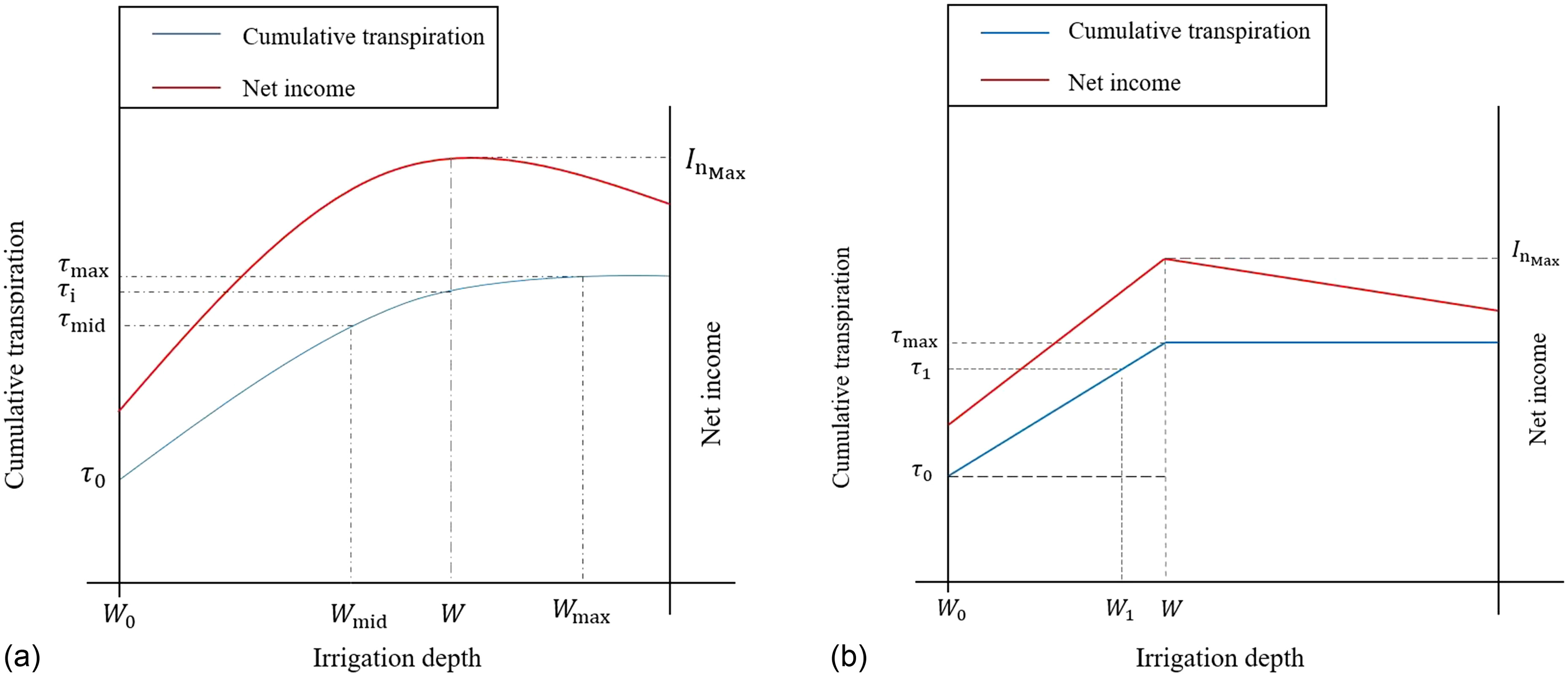
Two-Point Scheme
In this scheme, the relationship between and is described by two linear segments as
(6)
(7)
The former segment is defined by two points of corresponding to [Fig. 1(b)]: (, ) and (, ), where = (potential to determine the slope, . By substituting Eq. (6) into Eq. (1), the value of is determined at when the first derivative of Eq. (1) becomes zero
(8)
Hence, is determined as
(9)
(10)
Refilling Scheme
This scheme was proposed by Fujimaki et al. (2020). The value of is determined in a fixed irrigation interval to return , the volumetric water content at the end of each irrigation interval, to , the volumetric water content at field capacity, as follows:where = row spacing (cm); = width of root zone (cm); and = depth of plant root zone (cm)where , , and are fitting parameters. The WASH_2D model estimates using the two-dimensional water balance equation of the combined liquid and gaseous phases aswhere = time (s); = liquid water flux (); = water vapor flux (); and = horizontal distance and depth (cm), respectively; and is a sink term that refers to plant water uptake, which is described as (van Genuchten 1987)where , , and = reduction coefficient due to drought and salinity stresses, normalized root density distribution, and potential transpiration (), respectively. Parameter is expressed in the additive form aswhere , , and are fitting parameters. Parameter is calculated aswhere = fitting parameter; and = soil depth and depth below which roots exist (cm), respectively; and = horizontal distance from the plant (cm). Parameter in Eq. (14) is calculated using the well-known FAO56 PM equation as (Allen et al. 1998)where = reference evapotranspiration; and = basal crop coefficientwhere , , , , and are fitting parameters. The factors, and are expressed as functions of , rather than days after planting, to make the plant more dynamically respondent to both drought and salinity stresses. Further detail information of the WASH_2D model were presented by Fujimaki et al. (2014).
(11)
(12)
(13)
(14)
(15)
(16)
(17)
(18)
Simulation Procedure
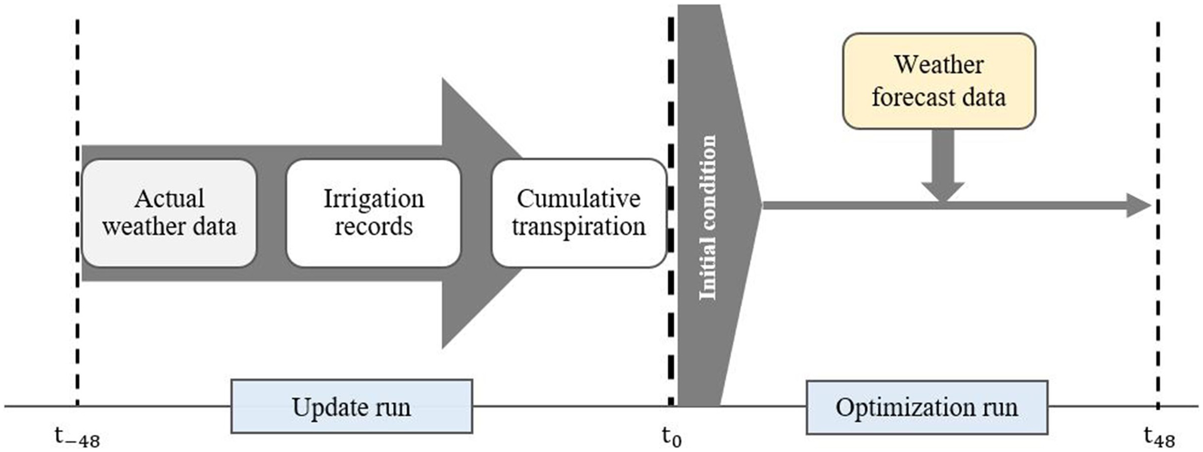
To determine , two steps were performed (Fig. 2). In Step 1, we ran the simulation to update the initial conditions using the information of the previous irrigation interval (48 h): irrigation records, meteorological data, and cumulative transpiration. In this step, was calculated for the refilling scheme to return updated values of to . In Step 2, the optimization was performed for both the three-point and two-point schemes using information from the update from Step 1 in addition to weather forecast data to determine values of that maximize in each irrigation interval. Weather forecast data were used to predict liquid water inputs from rain, evaporation from soil surface, and .
Field Evaluation
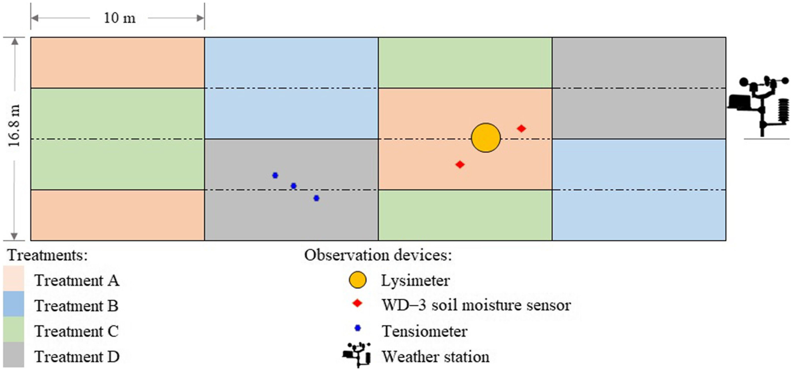
The proposed schemes were evaluated using a field experiment located in the Arid Land Research Center of Tottori University in 2021. It was carried out as a randomized complete block design with four independent blocks and the following four treatments (Fig. 3):
1.
Treatment A: was determined every 2 days using the three-point scheme.
2.
Treatment B: was determined every 2 days using the two-point scheme.
3.
Treatment C: was determined every 2 days to return to using the refilling scheme.
4.
Treatment D: was controlled by an automated system consisting of a solenoid valve, a CR300 series data logger (Campbell Scientific, Logan, Utah) and three tensiometers installed at a depth of 20 cm. Irrigation timing and were determined automatically by setting the scan interval for the measurement of average matric potential of the three tensiometers to 15 min and the trigger value to (Abd El Baki et al. 2020). This value was chosen to minimize downward percolation loss and to avoid drought stress, which occurs well below field capacity in sandy soils. We set up this treatment because it somewhat automatically meets crop water requirement in timely manner while minimizing deep percolation loss if the system is properly set. In Treatments A, B, and C, the irrigation interval was fixed at 2 days, because this sandy soil has low available water, and if the irrigation interval was set to three days, plants often would suffer from severe drought stress, which may negatively affect the final yield. If we set the irrigation interval at 1 day, Schemes A and B often gave zero recommended irrigation depth, which indicates that the interval is too short. In general, a 1-day interval may keep the soil wet longer, resulting in larger evaporation loss.
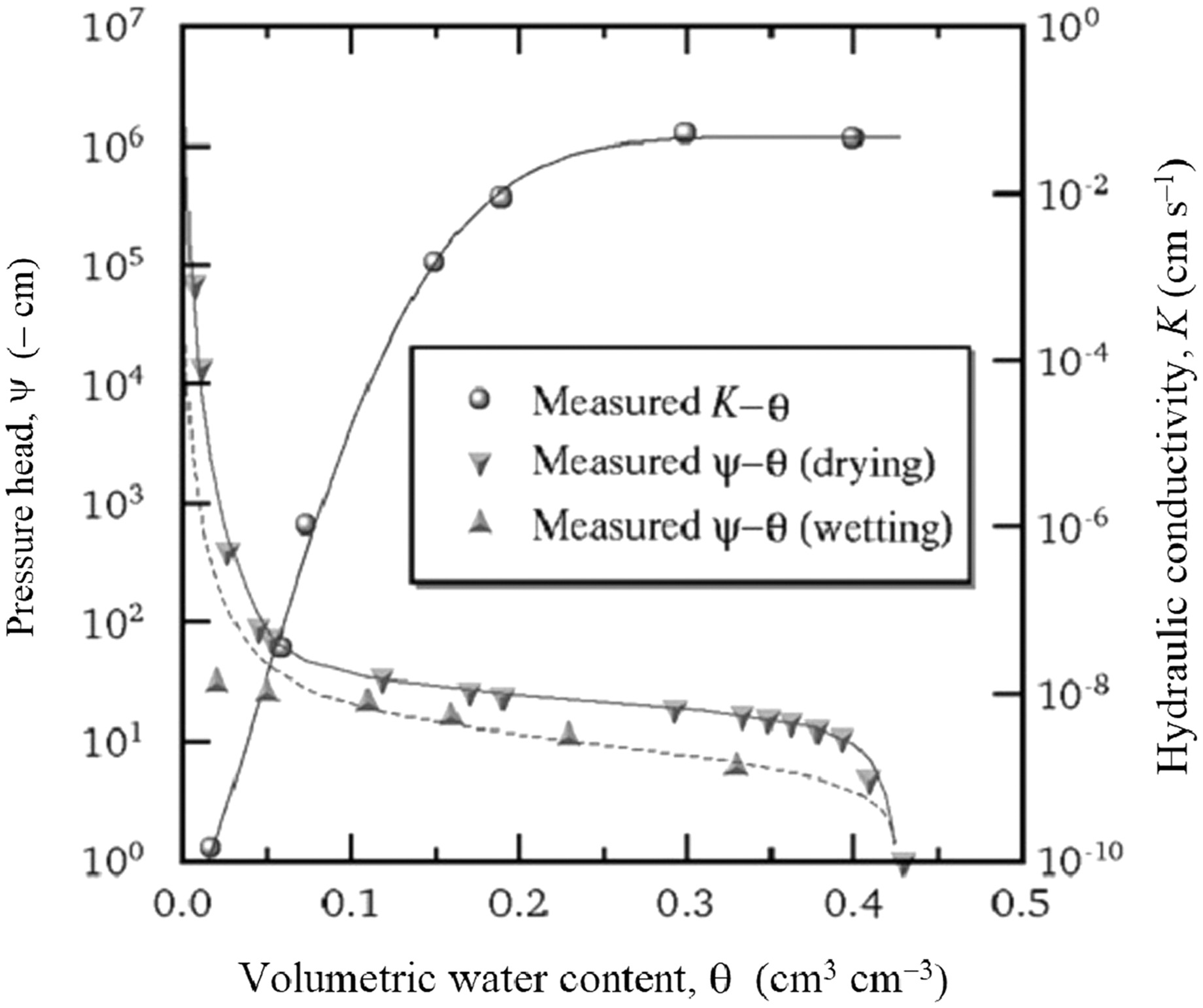
A drip irrigation network was installed, and each replicate was irrigated with seven drip tubes spaced at 60 cm intervals along 10 m. The emitter spacings and discharge rate were 20 cm and , respectively. The soil was sand (99.1% sand); the hydraulic properties are shown in Fig. 4.
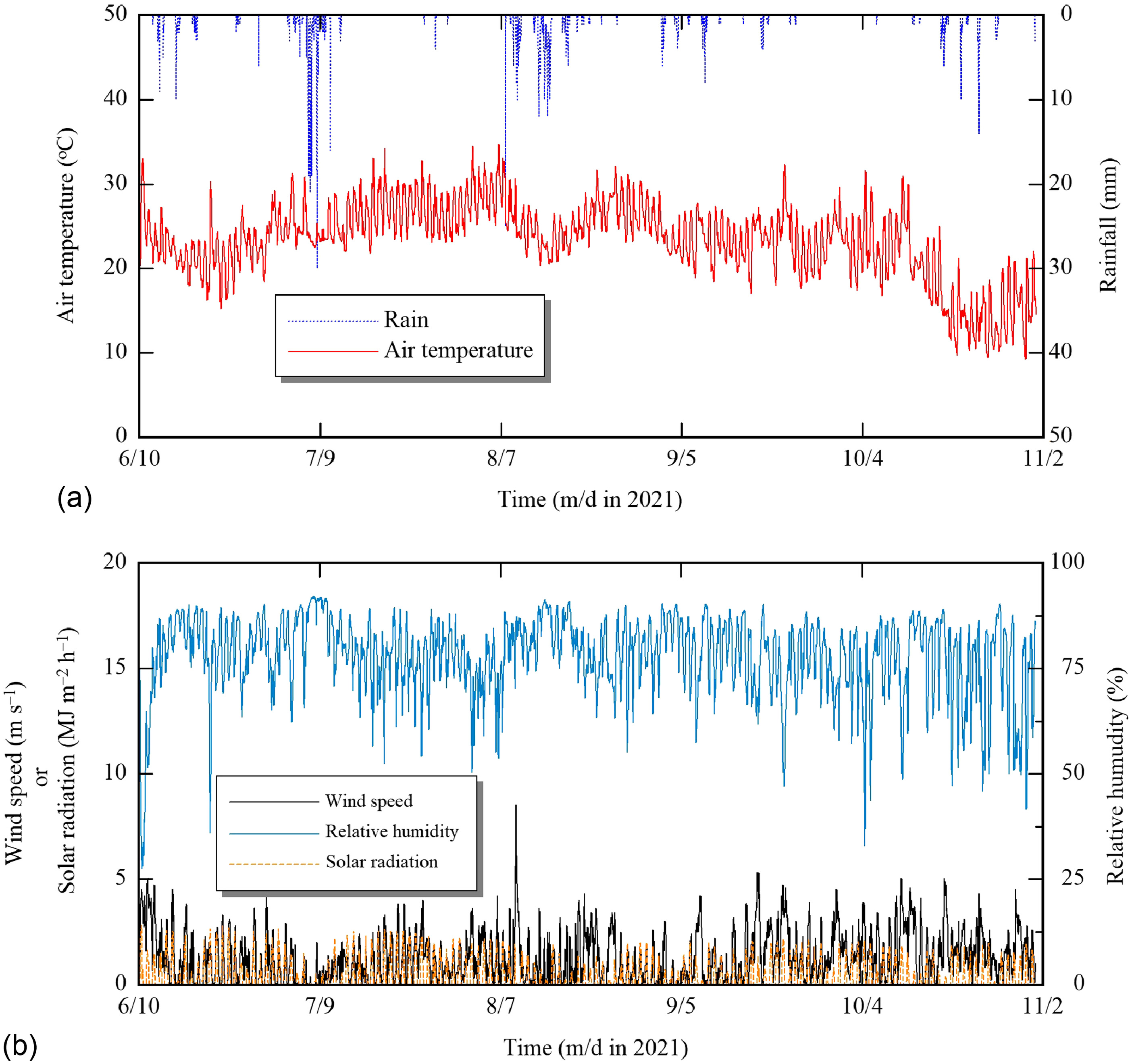
Actual weather data [air temperature (°C), rainfall (mm), wind speed (), solar radiation (), and relative humidity (%)] were collected from a weather station installed in the field (Fig. 5). Weather forecast data were accessed and downloaded from the website of Yahoo! Japan (Yahoo Japan Corporation 2022). Measured weather data were used to compute ET over the growing season. The Yahoo! website provides numerical values for all parameters required to compute except solar radiation. Instead, it provides nonnumerical forecasts of sky cover such as “rain,” “cloudy,” or “clear.” Those descriptions were used to calculate the solar radiation in accordance with Fujimaki et al. (2014). The wind speed values provided by the Yahoo! website refer to a standard height of 10 m, so those data were converted to 2-m heights based on the approach described by Allen et al. (1998).
The feasibility of the WASH_2D model to simulate soil water flow was evaluated as follows:
1.
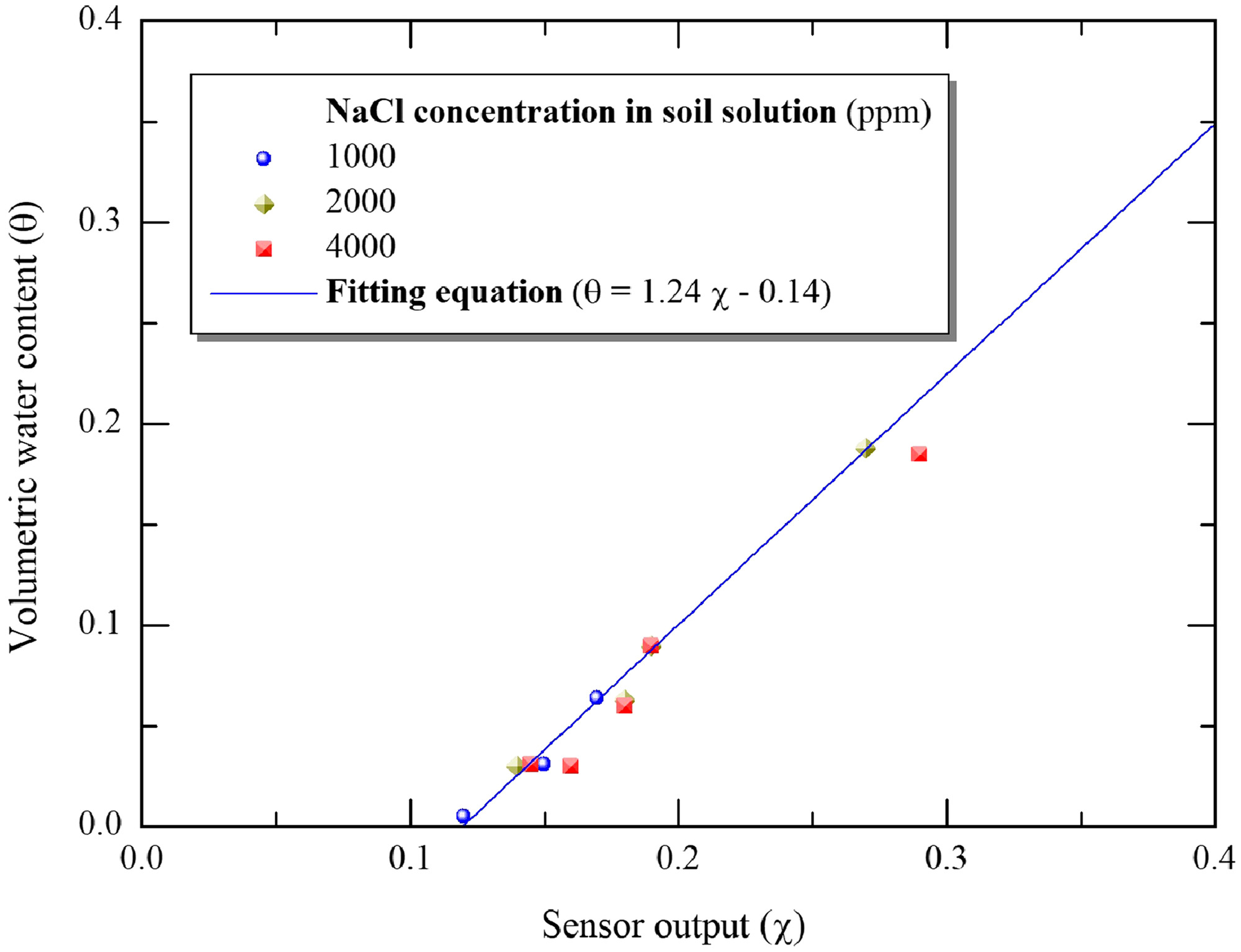
The simulated values of were compared with the measured values using two soil moisture sensors (WD-3-W-5Y, ARP, Horikawa, Hatano, Kanagawa, Japan) inserted 5 and 45 cm below the plant in two replicates. The sensor was calibrated for the Tottori sand (Fig. 6).
2.
The simulated values of were compared with the observed values. ET was measured using a weighing lysimeter with a diameter and depth of 1.5 and 2 m, respectively. The value of () was calculated using a water balance equation as follows:where = lysimeter water volume per unit lysimeter area (mm); = discrete time level; = precipitation (); = irrigation (); and = drainage from lysimeter (). The lysimeter weight was recorded at 5-min intervals. To reduce the measurement noise, we used the hourly moving averaged values.
(19)
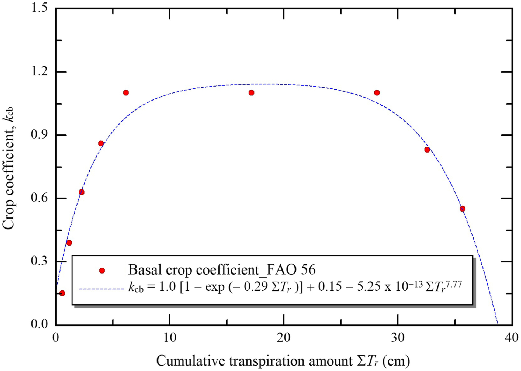
The cuttings of sweet potato [Ipomoea batatas (L.), cv. Kintoki] were transplanted on June 10 at 40 cm intervals along the drip tubes. The parameter values of the stress response function [Eq. (13)] were determined to , , and , from a pot experiment. The parameter values of the function [Eq. (16)] were obtained by fitting to those reported by Allen et al. (1998), assuming that during the initial, development, middle, and late stages was 2, 3, 4, and , respectively (Fig. 7). We estimated the net income by setting based on typical value of producer prices in 2020 (FAOSTAT 2021); was set to $0.0002/kg, similar to a case in Israel (Cornish et al. 2004); and was set to 0.003 (Siqinbatu et al. 2013).
Nitrogen-phosphorus-potassium (NPK) fertilizers were applied throughout the growing seasons in two forms: (1) a solid form in two types, and , at total rates of 60, 35, and , P, and K, respectively; and (2) liquid fertilizer () at total rates of 95, 15, and , P, and K, respectively (Laurie et al. 2012). The daily application rate of NPK liquid fertilizer was constant and equal among treatments. Plant samples were collected at 35, 53, 74, 97, 119, and 144 days after transplanting (DAT) to evaluate the plant growth in terms of leaf area index (LAI), biomass, and harvest index, defined as the ratio of dry weight (DW) of tubers (g) to the total plant dry weight (g) (Bourke 1985). Plants were harvested on November 1, 2021. Yield and its components—dry weight of fresh leaves (), dry weight of shriveled leaves (), fresh weight (FW) of tubers (), dry weight of dry tubers (), dry weight of stem (), and total biomass ()—were analyzed statistically using a randomized complete block design. The ANOVA test was conducted using SPSS version 26.0 software to estimate the significant differences among the four treatments.
Results and Discussion
Plant Growth and Yield
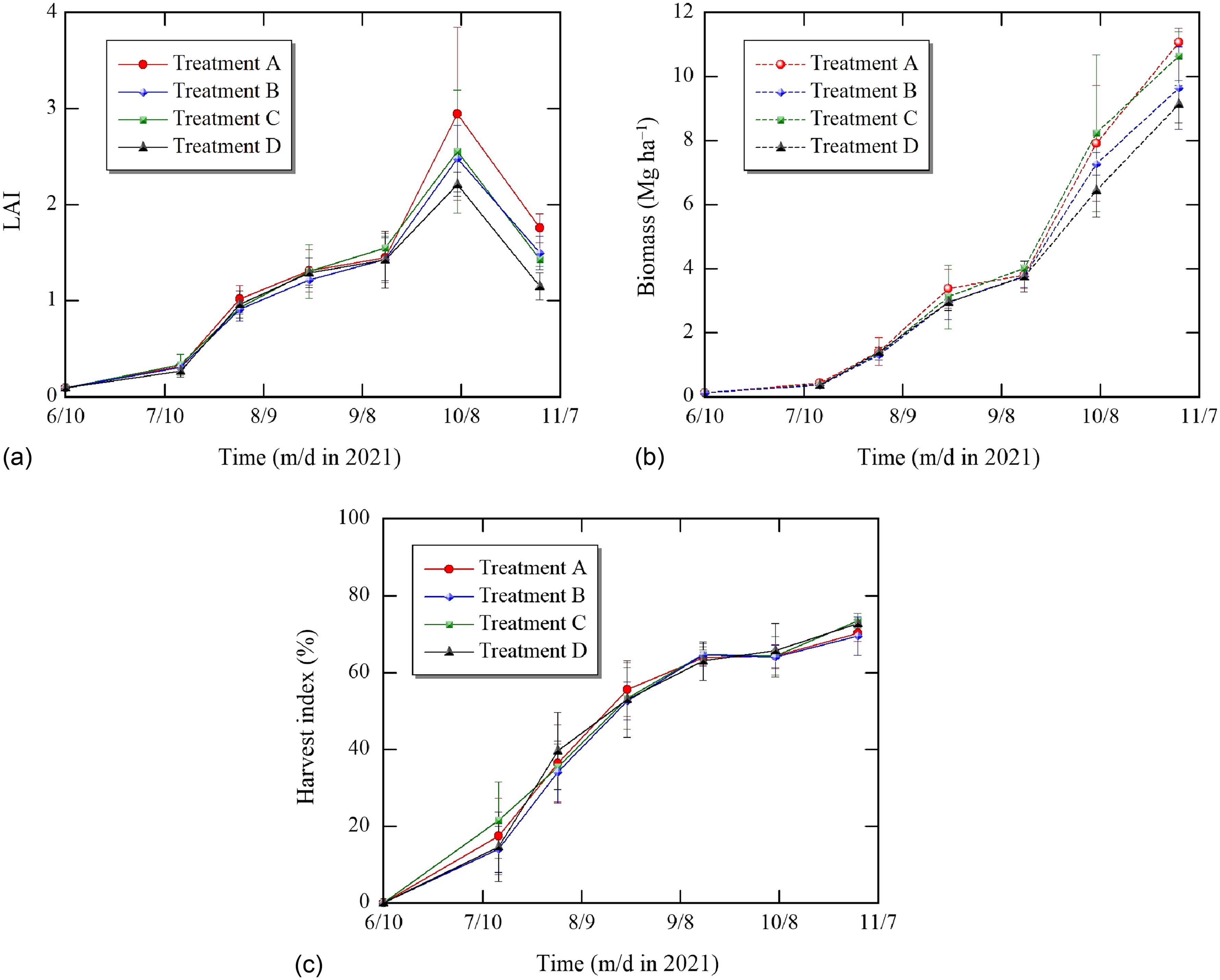
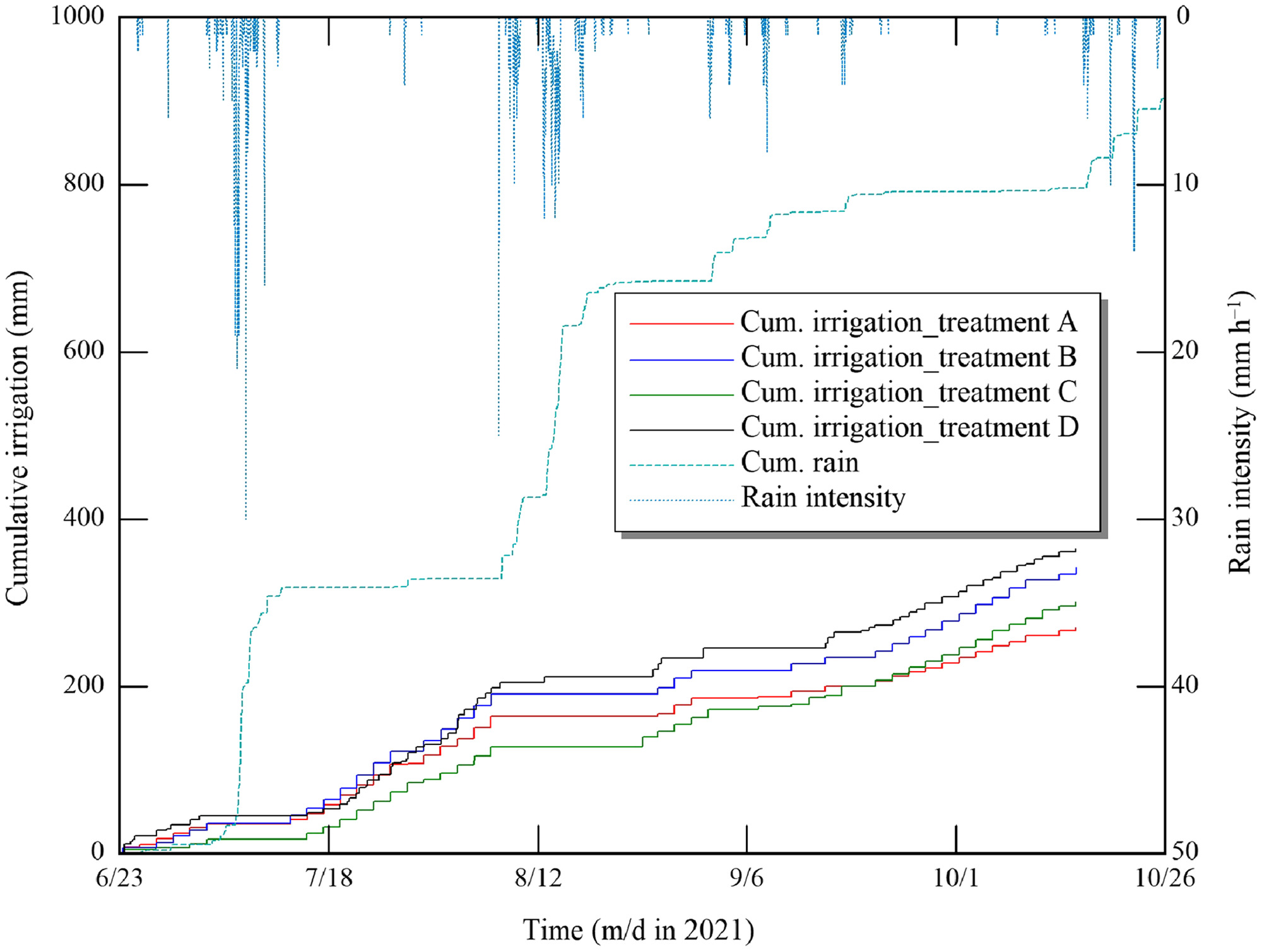
The LAI, biomass, and harvest index as functions of time are shown in Fig. 8. The maximum mean values of LAI for Treatments A, B, C, and D were 2.9, 2.5, 2.6, and 2.2, respectively, which were measured at 119 DAT (October 7), after which values declined. The harvest index indicated similar values for Treatments A, B, C, D, i.e., 70%, 69%, 74%, and 73%, respectively. The results of LAI and harvest index agreed with those reported by Bourke (1985). The growth rate of biomass, which is the slope of Fig. 8(b), was stagnant from 74 DAT (August 23) to 97 DAT (September 15), with a mean value of . This likely was due to lesser solar radiation and heavy rainfall events that may have caused deep nutrient leaching beyond the plant rootzone. After 97 DAT, the growth rate recovered and varied among the treatments, which may have been due to the effect of irrigation on nutrients uptake by plants. Treatment C tended to have less water applied than other treatments until August 6, after which irrigation gradually increased (Fig. 9). This may have led to less nutrient leaching in Treatment C than in other treatments, and partly offset negative effects of drought stress in the early stage. As a result, the fresh tuber yield was 19.7, 19.4, 19.7 and for Treatments A, B, C and D, respectively. The statistical analysis of yield components is presented in Table 1. There were no significant differences for whole components among the treatments (). Treatment A had a higher dry mass of leaves and LAI. Treatments A and C had slightly higher values of fresh tuber yield than the other treatments, probably due to higher nutrient uptake, which may have increased the photosynthetic rates, which enhanced the transport of carbohydrates from the leaves to the tubers (Abd El-Baky et al. 2010).
| Variable | Treatment | ANOVA ( probability) | |||
|---|---|---|---|---|---|
| A | B | C | D | ||
| DW, green leaves () | 0.46 | ||||
| DW, shriveled leaves () | 0.33 | ||||
| DW, stem () | 0.34 | ||||
| FW, tubers () | 0.06 | ||||
| DW, tubers () | 0.14 | ||||
| Biomass () | 0.23 | ||||
| LAI | 0.46 | ||||
Note: Treatments A, B, C, and D refer to three-point, two-point, refilling, and automated irrigation schemes, respectively. Data are mean values ± standard error.
Net Income
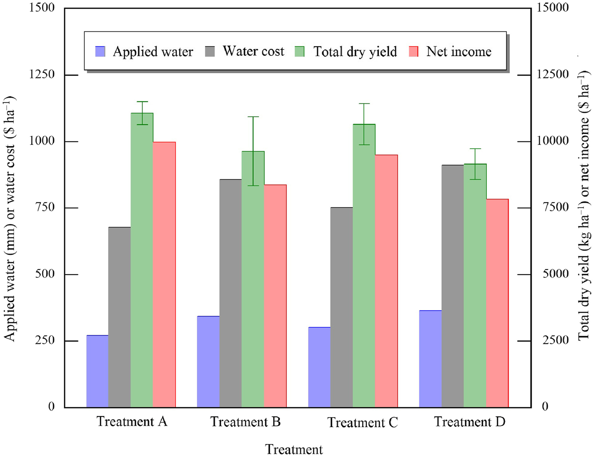
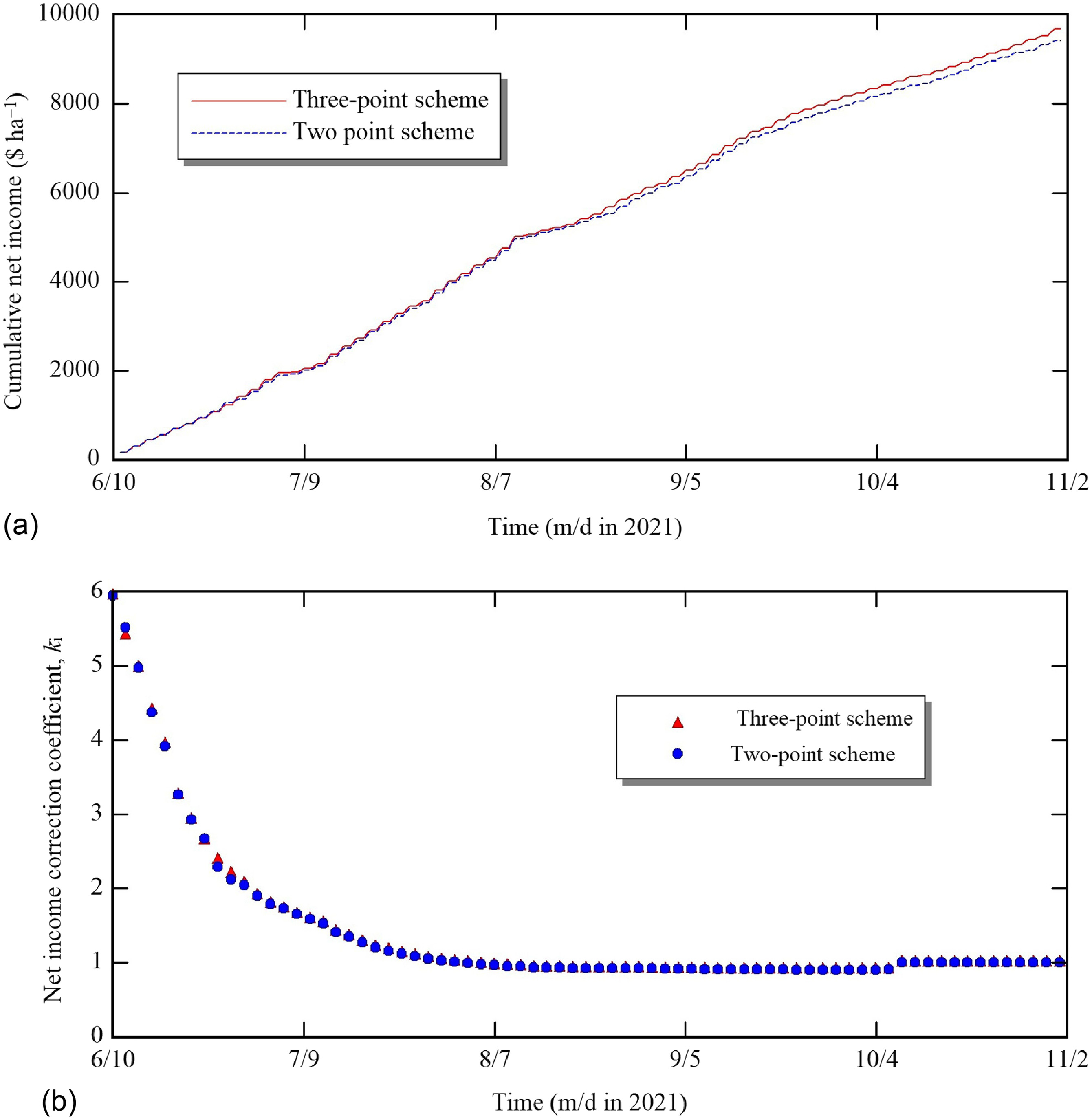
We focused on the cost of applied water to motivate farmers to save water. The main concern of farmers is not water productivity (yield per applied water), but net income (Fujimaki et al. 2014). Hence, the effectiveness of the proposed schemes in terms of net income is presented in Fig. 10. Treatment A achieved net income by 16%, 5% and 22% higher than that of Treatments B, C, and D, respectively. This was due to producing 13%, 4% and 17% higher biomass and applying 24%, 11%, and 27% less water than in Treatments B, C, and D, respectively. One of the major advantages of the three-point and two-point schemes is maximizing the farmers’ net income in each irrigation event, rather than the seasonal net income, as employed in other studies (e.g., Wang and Cai 2009). To confirm that simulated net income matched the observed value, the cumulative virtual net income for the three-point and two-point schemes is illustrated in Fig. 11(a). The total simulated net income achieved for the three-point and two-point schemes was $9,677 and , respectively, whereas the actual values were $9,983 and , respectively. The optimization gave almost the same gross net income as the actual values. The values decreased sharply from 6 to 1 as the crop grew [Fig. 11(b)].
Accuracy of Numerical Simulation
Evapotranspiration
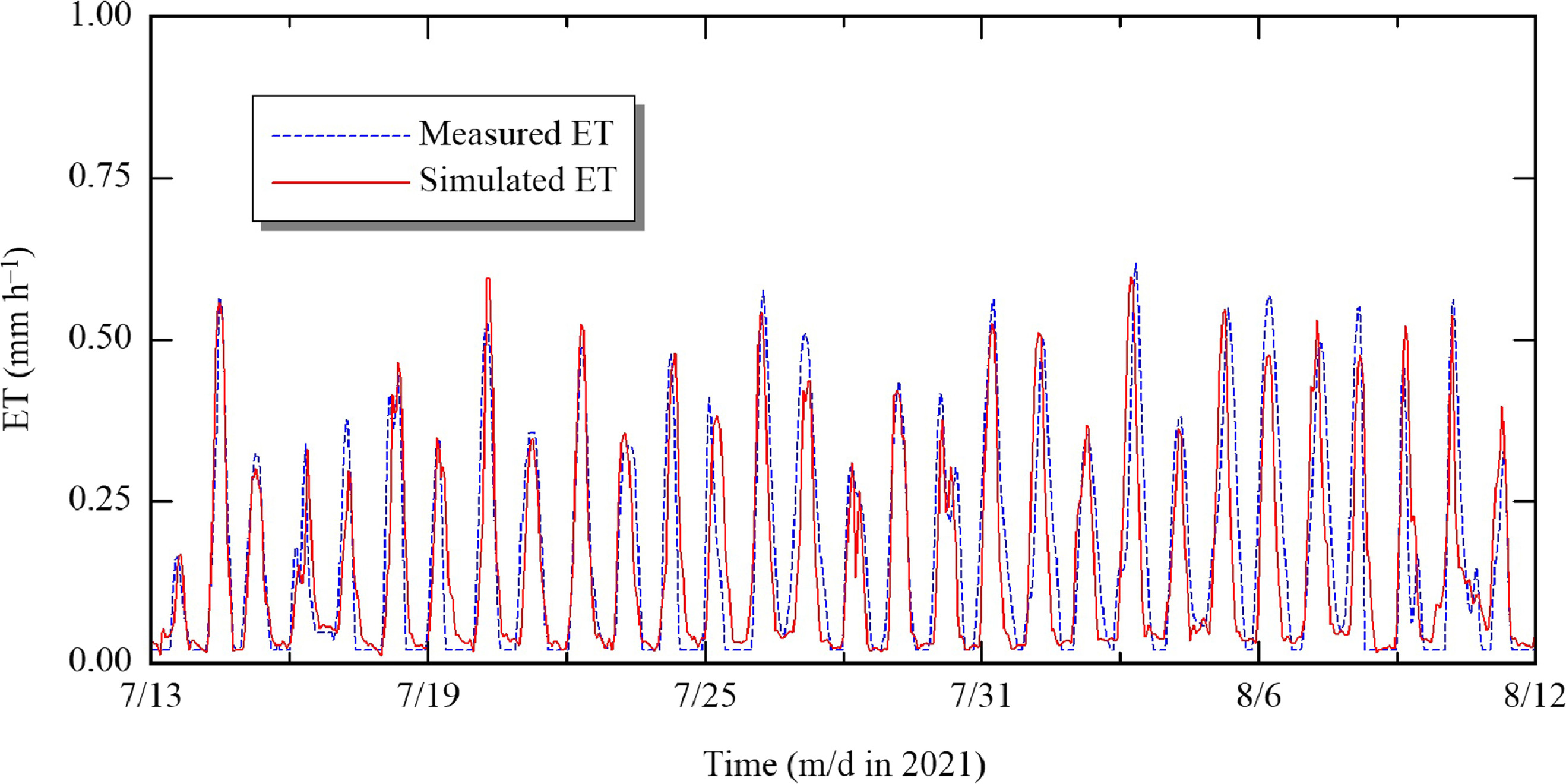
The fluctuation of simulated ET was compared with the observed value measured with a weighing lysimeter (Fig. 12). The model tended to underestimate ET values, with a RMS error (RMSE) of . The discrepancy may have been caused partly by disturbance of weight measurement by wind over [Fig. 5(b)], as reported by Schrader et al. (2013) and Lorite et al. (2012), particularly because the level of lysimeter surface was slightly higher than the surrounding field, by 3–5 cm. This also may have caused the drip tubes to touch the surface of the lysimeter, affecting the weight measurement due to tension change caused by temperature fluctuation.
Volumetric Water Content
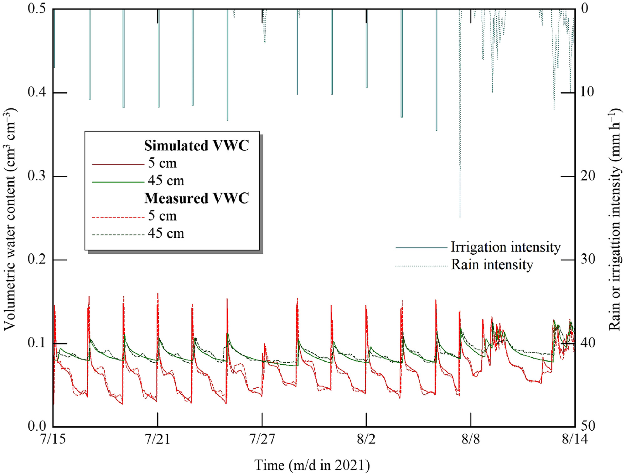
The measured and simulated for the period July 15–August 14 is illustrated in Fig. 13. We showed the response of to both irrigation and rainfall events in Treatment A for top and deep soil layers below the plant. The model accurately simulated , with a RMSE of 0.015 and compared with the measured values at 5 and 45 cm below an emitter, respectively. These results agreed with those reported by Fujimaki et al. (2014) and Abd El Baki et al. (2020) for Tottori sand and by Zhu et al. (2018) for loamy soil with the same bulk density as Tottori sand.
Impact of Short Weather Forecast on Irrigation Optimization
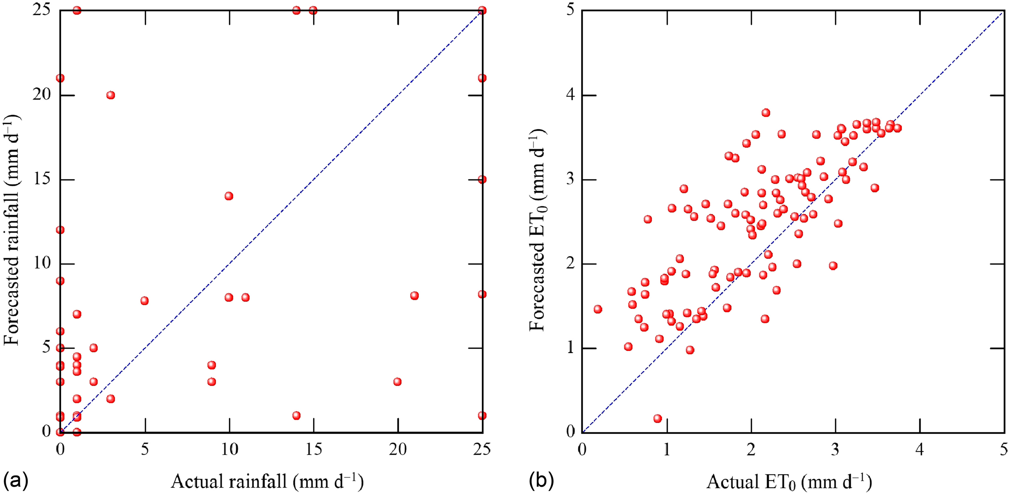
To check the accuracy of rain forecasts and WF data, which greatly affected the determination of , we compared daily forecasted rainfall and daily forecasted with the daily observed values (Fig. 14). As WFs were downloaded in the morning of each irrigation day at 09:00 until the day end at 23:59, the term “daily” means from 9:00 to 24:00. Total measured and forecasted rainfall across the growing season were similar, 598 and 648 mm, respectively. In contrast, the forecasted amount of each rainfall event often deviated greatly from the measured amounts. The total number of measured and forecasted rainfall events were 39 and 52 over 120 days, respectively. Setting effective rainfall to , the RMSE between measured and forecasted values was , in which 17% and 15% of rain events exceeded this setting (25 mm d−1), respectively. This is consistent with the findings of Shrestha et al. (2013), who found that the RMSE for daily forecasted rainfall ranged from 4.67 to . Relative RMSE, which is the ratio of the average value to the RMSE, was 0.77. Those underestimations and overestimations of rain may have caused overestimation and underestimation of , respectively. On the other hand, daily calculated using hourly forecasted values generally was overestimated, with a RMSE of compared with calculated using the measured values. Relative RMSE was 0.81. Those overestimations may have caused overestimations of . This likely was due to overestimation of wind speed, with a RMSE of , and underestimation of relative humidity, with a relative RMSE of 1.17. These results agreed with the possible reasons reported by Lorite et al. (2015), who observed that high wind speed and close proximity to the sea caused larger errors in estimation, and by Xiong et al. (2016), who indicated that relative humidity is an important factor to estimate in humid regions. An interval longer than 2 days in this study is appropriate in finer-textured soils, but accuracy at longer forecast horizons would be even lower than that at 2 days. Gowing and Ejieji (2001) observed that using short-term weather forecasts (up to 5 days ahead) is useful to save both cost and irrigation depth, and thereby increases net income in wet seasons, whereas it led to improved water-use efficiency of limited water supply in dry seasons. Cai et al. (2011) reported that even an imperfect 1-week forecast still was valuable in terms of both profit gain and water saving. In parallel to the present study, Abd El Baki and Fujimaki (2021a) observed that using 1-day weather forecasts led to more-accurate estimates of , with a RMSE for a sandy filed. We expect that the accuracy of numerical weather forecast will continue improving with the use of faster supercomputers using finer grids and improved submodels. Despite the current accuracy of WFs, they may still have benefits for determining irrigation depths.
Advantages and Disadvantages of the Proposed Schemes
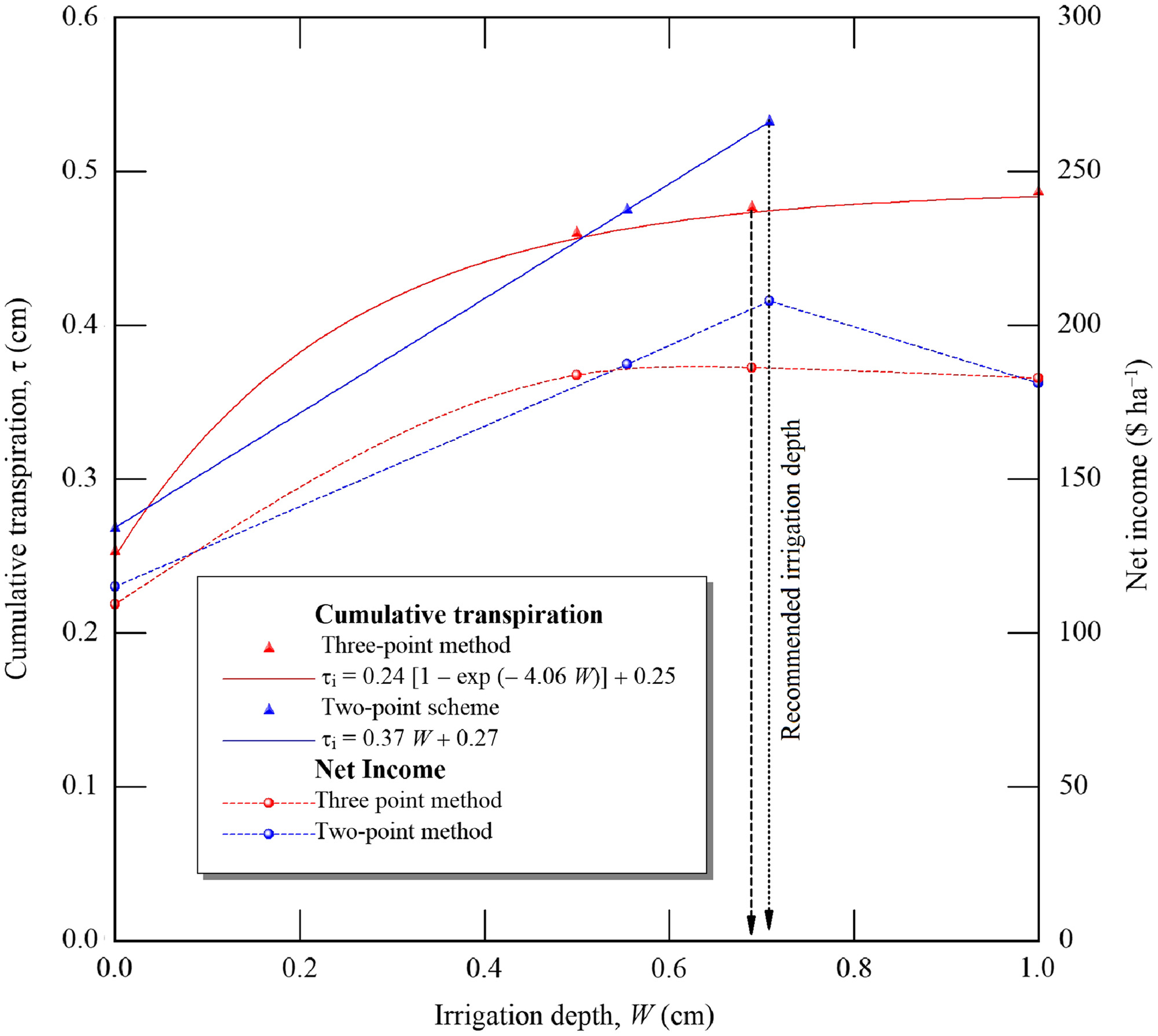
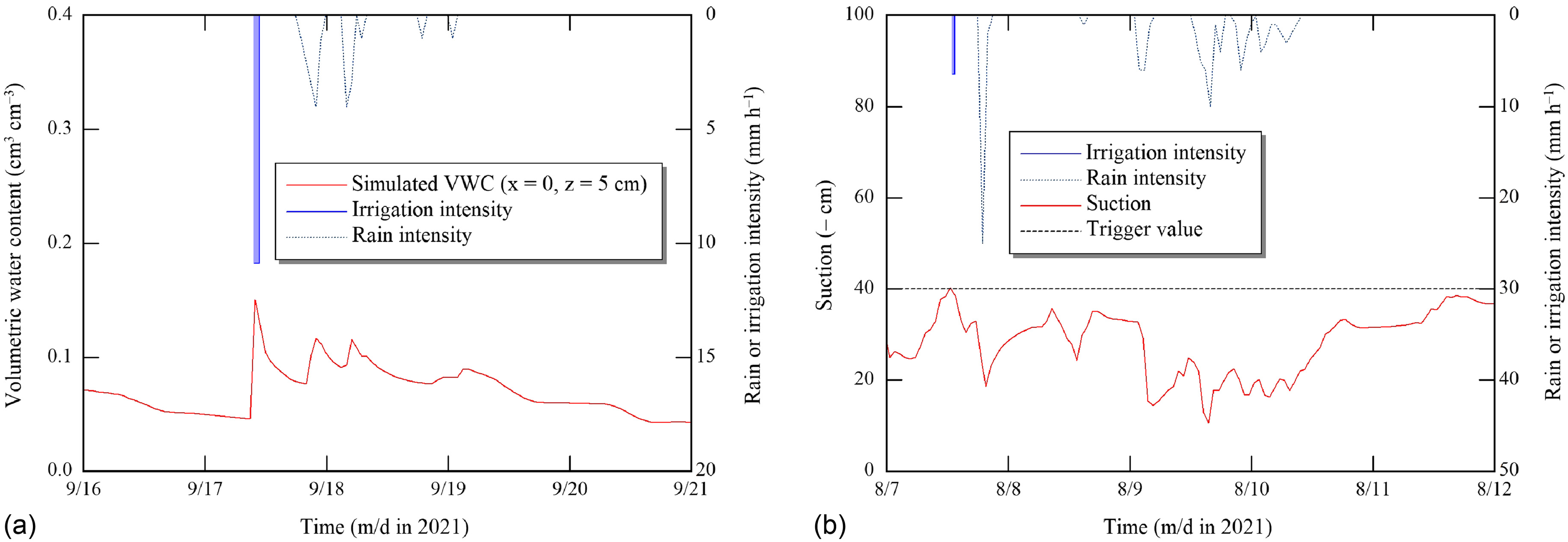
The combination of numerical simulation, volumetric water pricing, and weather forecasts could be useful in making optimal irrigation decisions. In this regard, Fig. 15 shows an example of determining using the three-point and two-point schemes on July 15. Both gave similar recommended values of , as 0.69 and 0.71 cm at a maximum value of , respectively. We found that both schemes gave similar values of recommended only when irrigation was not performed in the previous event. In other cases, the two-point scheme often gave a higher , partly due to inappropriate setting of (0.55 cm in Fig. 15), which is the main drawback of the scheme (Abd El Baki and Fujimaki 2021). Scheme B may give higher net income than other treatments only when the relationship between and cumulative transpiration can be described by two linear segments (trapezoidal). Our results indicate that the assumption invoked in Scheme B generally was inappropriate in the experimental condition. On the same day, the refilling scheme suggested refilling water into the root zone with for the next 2 days. The drawback of the refilling scheme is that it neglects the near-future rainfall events [Fig. 16(a)]. For example, the refilling scheme suggested to return to on September 17. Irrigation began at 09:00, and rainfall started at 17:00. Such a case occurred only once across the entire season. This may be another reason why Treatment C gave higher values of than Treatment B. The automated irrigation scheme also tended to neglect the near-forecast rainfall events [Fig. 16(b)]. On August 7, water was applied automatically with at 13:00 when the trigger suction value approached . Soon after that, 2.5 cm of rainfall occurred at 17:00. This overirrigation repeated six times, which may be a reason why Treatment D applied more water and leached nutrients beyond the plant rootzone than did the other schemes. Automated irrigation systems also are sensitive to the selection of optimum trigger suction value, which requires additional field studies (Migliaccio et al. 2010). If one tensiometer was set under a clogged emitter, the observed suction value could result in the application of more water. Thus, the proposed simulation schemes, as an innovative technology considering weather forecasts, would be more affordable to farmers to maximize their net income or, at the very least, provide promising trends for optimizing water use. The proposed schemes are a type of appropriate and/or intermediate technology (Schumacher 1999) that farmers can adopt easily after being trained using the most effective agricultural extension methods, such as demonstration, farmer-to-farmer, and household extension methods.
Conclusions
The use of numerical simulation considering weather forecasts and volumetric water prices could maximize farmers’ net income compared with automated irrigation. Both the two-point and the three-point schemes aimed to determine irrigation depth to achieve maximum net income in each irrigation interval. As a result of a field experiment, we found that the three-point scheme was the most effective in terms of net income. The cumulative simulated net income with the three- and two-point schemes at the end of the growing season fairly matched the measured values. Although the refilling scheme attained the second highest net income, it sometimes could not respond to the near-future rainfall events, which may waste water and deeply leach nutrients beyond the rootzone. Similarly, automated irrigation wasted more water and cause more nutrient leaching than did the other treatments. The model could simulate and ET in fair agreement with observed values. Estimates of daily using WF data were affected by overestimation, with a RMSE of . Total forecasted rainfall matched with the measured value, but although weather forecasts frequently failed to predict the occurrence of rainfall events. These simulation schemes will be practiced widely in the future under semiarid conditions and compared with rainfed agriculture. In general, the use of numerical simulation and weather forecasts can increase farmers’ net income under volumetric water pricing. In addition, farmers may save the high cost of purchasing, installing, and maintain automated systems.
Data Availability Statement
Some data, models, or code that support the findings of this study are available from the corresponding author upon reasonable request, including the WASH_2D model, simulation data, weather forecasts, meteorological data, irrigation records, observed data of soil moisture and evapotranspiration, and yield and its components.
Acknowledgments
We thank all members of irrigation and drainage lab of the Arid Land Research Center for their assistance in data collection and other processes that led to successful results.
References
Abd El Baki, H. M., and H. Fujimaki. 2021a. “Determining economical irrigation depths in a sandy field using a combination of weather forecast and numerical simulation.” Water 13 (Nov): 3403. https://doi.org/10.3390/w13233403.
Abd El Baki, H. M., and H. Fujimaki. 2021b. “An evaluation of a new scheme for determination of irrigation depths in the Egyptian Nile Delta.” Water 13 (Sep): 2181. https://doi.org/10.3390/w13162181.
Abd El Baki, H. M., H. Fujimaki, I. Tokumoto, and T. Saito. 2017. “Determination of irrigation depths using a numerical model of crop growth and quantitative weather forecast and evaluation of its effect through a field experiment for potato.” J. Jpn. Soc. Soil Phys. 136 (Apr): 15–24. https://doi.org/10.34467/jssoilphysics.136.0_15.
Abd El Baki, H. M., H. Fujimaki, I. Tokumoto, and T. Saito. 2018a. “A new scheme to optimize irrigation depth using a numerical model of crop response to irrigation and quantitative weather forecasts.” Comput. Electron. Agric. 150 (5): 387–393. https://doi.org/10.1016/j.compag.2018.05.016.
Abd El Baki, H. M., H. Fujimaki, I. Tokumoto, and T. Saito. 2018b. “Optimizing irrigation depth using a plant growth model and weather forecast.” J. Agric. Sci. 10 (7): 55–66. https://doi.org/10.5539/jas.v10n7p55.
Abd El Baki, H. M., M. Raoof, and H. Fujimaki. 2020. “Determining irrigation depths for soybean using a simulation model of water flow and plant growth and weather forecasts.” Agronomy 10 (3): 369. https://doi.org/10.3390/agronomy10030369.
Abd El-Baky, M. M. H., A. A. Ahmed, M. A. El-Nemr, and M. F. Zaki. 2010. “Effect of potassium fertilizer and foliar zinc application on yield and quality of sweet potato.” Res. J. Agric. Biol. Sci. 6 (4): 386–394.
Ahuja, L. R., K. W. Rojas, J. D. Hanson, M. J. Shaffer, and L. Ma. 2000. Root zone water quality model: Modeling management effects on water quality and crop production. Littleton, CO: Water Resources Publications.
Allen, R., L. Pereira, D. Raes, and M. Smith. 1998. Crop evapotranspiration: Guidelines for computing crop water requirements, 135–142. Rome: FAO.
Bauer, P., A. Thorpe, and G. Brunet. 2015. “The quiet revolution of numerical weather prediction.” Nature 525 (Aug): 47–55. https://doi.org/10.1038/nature14956.
Bourke, R. M. 1985. “Influence of nitrogen and potassium fertilizer on growth of sweet potato (Ipomoea batatas) in Papua New Guinea.” Field Crops Res. 12 (Jan): 363–375. https://doi.org/10.1016/0378-4290(85)90081-4.
Cai, J. B., Y. Liu, T. Lei, and L. S. Pereira. 2007. “Estimating reference evapotranspiration with the FAO Penman–Monteith equation using daily weather forecast messages.” Agric. For. Meteorol. 145 (1): 22–35. https://doi.org/10.1016/j.agrformet.2007.04.012.
Cai, X., M. I. Hejazi, and D. Wang. 2011. “Value of probabilistic weather forecasts: Assessment by real-time optimization of irrigation scheduling.” J. Water Resour. Plann. Manage. 137 (5): 391–403. https://doi.org/10.1061/(asce)wr.1943-5452.0000126.
Cammarano, D., J. Payero, B. Basso, P. Wilkens, and P. Grace. 2012. “Agronomic and economic evaluation of irrigation strategies on cotton lint yield in Australia.” Crop Pasture Sci. 63 (Feb): 647–655. https://doi.org/10.1071/CP1202.
Cornish, G., B. Bosworth, and C. Perry. 2004. Water charging in irrigated agriculture—An analysis of international experience, 19–26. Rome: FAO.
Davis, S. L., and M. D. Dukes. 2010. “Irrigation scheduling performance by evapotranspiration-based controllers.” Agric. Water Manage. 98 (1): 19–28. https://doi.org/10.1016/j.agwat.2010.07.006.
English, M. 1990. “Deficit irrigation. I: Analytical framework.” J. Irrig. Drain. Eng. 116 (3): 399–412. https://doi.org/10.1061/(ASCE)0733-9437(1990)116:3(399).
Evett, S. R., R. C. Schwartz, N. T. Mazahrih, M. A. Jitan, and I. M. Shaqir. 2011. “Soil water sensors for irrigation scheduling: Can they deliver a management allowed depletion?” Acta Hortic. 888 (26): 231–237. https://doi.org/10.17660/ActaHortic.2011.888.26.
FAOSTAT (Food and Agriculture Organization Corporate Statistical Database). 2021. “Producer prices.” Accessed June 23, 2021. https://www.fao.org/faostat/en/#data/PP.
Farooq, M., M. Hussain, S. Ul-Allah, and K. H. M. Siddique. 2019. “Physiological and agronomic approaches for improving water-use efficiency in crop plants.” Agric. Water Manage. 219 (Sep): 95–108. https://doi.org/10.1016/j.agwat.2019.04.010.
Fujimaki, H., H. M. Abd El Baki, S. M. Mahdavi, and H. Ebrahimian. 2020. “Optimization of irrigation and leaching depths considering the cost of water using WASH_1D/2D models.” Water 12 (9): 2549. https://doi.org/10.3390/w12092549.
Fujimaki, H., I. Tokumoto, T. Saito, M. Inoue, M. Shibata, T. Okazaki, K. Nagaz, and F. El Mokh. 2014. “Determination of irrigation depths using a numerical model and quantitative weather forecast and comparison with an experiment.” In Vol. 5 of Practical applications of agricultural system models to optimize the use of limited water, edited by L. R. Ahuja, L. Ma, and R.J. Lascano, 209–235. Madison, WI: ACSESS.
Garcia-Vila, M., and E. Fereres. 2012. “Combining the simulation crop model AquaCrop with an economic model for the optimization of irrigation management at farm level.” Eur. J. Agron. 36 (May): 21–31. https://doi.org/10.1016/j.eja.2011.08.003.
Gedam, S., S. Pallam, B. V. N. P. Kambhammettu, V. Anupoju, and S. K. Regonda. 2022. “Investigating the accuracies in short-term weather forecasts and its impact on irrigation practices.” J. Water Resour. Plann. Manage. 149 (2): 04022079. https://doi.org/10.1061/JWRMD5.WRENG-5644.
Ghazichaki, Z. H., and M. J. Monem. 2019. “Development of quantified model for application of control systems in irrigation networks by system dynamic approach.” Irrig. Drain. 68 (12): 433–442. https://doi.org/10.1002/ird.2331.
Glória, A., C. Dionísio, C. Simões, J. Cardoso, and P. Sebastião. 2019. “Water management for sustainable irrigation systems using internet-of-things.” Sensors 20 (14): 1402. https://doi.org/10.3390/s20051402.
Gowing, J. W., and C. J. Ejieji. 2001. “Real-time scheduling of supplemental irrigation for potatoes using a decision model and short-term weather forecasts.” Agric. Water Manage. 47 (2): 137–153. https://doi.org/10.1016/s0378-3774(00)00101-3.
Gu, Z., Z. Qi, R. Burghate, S. Yuan, X. Jiao, and J. Xu. 2020. “Irrigation scheduling approaches and applications: A review.” J. Irrig. Drain. Eng. 146 (6): 04020007. https://doi.org/10.1061/(ASCE)IR.1943-4774.0001464.
Jalil, A., F. Akhtar, and U. K. Awan. 2020. “Evaluation of the AquaCrop model for winter wheat under different irrigation optimization strategies at the downstream Kabul River Basin of Afghanistan.” Agric. Water Manage. 240 (Jun): 106321. https://doi.org/10.1016/j.agwat.2020.106321.
Jamal, A., R. Linker, and M. Housh. 2019. “Optimal irrigation with perfect weekly forecasts versus imperfect seasonal forecasts.” J. Water Resour. Plann. Manage. 145 (5): 06019003. https://doi.org/10.1061/(ASCE)WR.1943-5452.0001066.
Jones, J. W., G. Hoogenboom, C. H. Porter, K. J. Boote, W. D. Batchelor, L. A. Hunt, P. W. Wilkens, U. Singh, A. J. Gijsman, and J. T. Ritchie. 2003. “The DSSAT cropping system model.” Europ. J. Agronomy 18 (Sep): 235–265. https://doi.org/10.1016/S1161-0301(02)00107-7.
Kumar, H., P. Srivastava, J. Lamba, E. Diamantopoulos, B. Ortiz, G. Morata, B. Takhellambam, and L. Bondesan. 2022. “Site-specific irrigation scheduling using one-layer soil hydraulic properties and inverse modeling.” Agric. Water Manage. 273 (Apr): 107877. https://doi.org/10.1016/j.agwat.2022.107877.
Laurie, S. M., M. Faber, P. J. van Jaarsveld, R. N. Laurie, C. P. du Plooy, and P. C. Modisane. 2012. “β-Carotene yield and productivity of orange-fleshed sweet potato (Ipomoea batatas L. Lam.) as influenced by irrigation and fertilizer application treatments.” Sci. Hortic. 142 (Jul): 180–184. https://doi.org/10.1016/j.scienta.2012.05.017.
Liu, C., Z. Qi, Z. Gu, D. Gui, and F. Zeng. 2017. “Optimizing irrigation rates for cotton production in an extremely arid area using RZEWM2-simulated water stress.” Trans. ASABE 60 (5): 1–14. https://doi.org/10.13031/trans.12365.
Lorite, I. J., J. M. Ramírez-Cuesta, M. Cruz-Blanco, and C. Santos. 2015. “Using weather forecast data for irrigation scheduling under semi-arid conditions.” Irrig. Sci. 33 (5): 411–427. https://doi.org/10.1007/s00271-015-0478-0.
Lorite, I. J., C. Santos, L. Testi, and E. Fereres. 2012. “Design and construction of a large weighing lysimeter in an almond orchard.” Span. J. Agric. Res. 10 (1): 238–250. https://doi.org/10.5424/sjar/2012101-243-11.
Luo, Y., S. Traore, X. Lyu, W. Wang, Y. Wang, Y. Xie, X. Jiao, and G. Fipps. 2015. “Medium range daily reference evapotranspiration forecasting by using ANN and public weather forecasts.” Water Resour. Manage. 29 (Jul): 3863–3876. https://doi.org/10.1007/s11269-015-1033-8.
Migliaccio, K. W., B. Schaffer, J. H. Crane, and F. S. Davies. 2010. “Plant response to evapotranspiration and soil water sensor irrigation scheduling methods for papaya production in South Florida.” Agric. Water Manage. 97 (Sep): 1452–1460. https://doi.org/10.1016/j.agwat.2010.04.012.
Munoz-Carpena, R., M. D. Dukes, Y. Li, and W. Klassen. 2008. “Design and field evaluation of a new controller for soil-water based irrigation.” Appl. Eng. Agric. 24 (Aug): 183–191. https://doi.org/10.13031/2013.24266.
Munoz-Carpena, R., Y. C. Li, W. Klassen, and M. D. Dukes. 2005. “Field comparison of tensiometer and granular matrix sensor automatic drip irrigation on tomato.” HortTechnology 15 (3): 584–590. https://doi.org/10.21273/HORTTECH.15.3.0584.
Nijbroek, R., G. Hoogenboom, and G. H. Jones. 2003. “Optimizing irrigation management for a spatially variable soybean field.” Agric. Syst. 76 (1): 359–377. https://doi.org/10.1016/S0308-521X(02)00127-0.
Payero, J. O., and S. Irmak. 2013. “Daily energy fluxes, evapotranspiration and crop coefficient of soybean.” Agric. Water Manage. 129 (6): 31–43. https://doi.org/10.1016/j.agwat.2013.06.018.
Perera, K. C., A. W. Western, B. Nawarathna, and B. George. 2014. “Forecasting daily reference evapotranspiration for Australia using numerical weather prediction outputs.” Agric. For. Meteorol. 194 (3): 50–63. https://doi.org/10.1016/j.agrformet.2014.03.014.
Raes, D., P. Steduto, T. C. Hsiao, and E. Fereres. 2009. “AquaCrop—The FAO crop model to simulate yield response to water: II. Main algorithms and software description.” Agron. J. 101 (Jul): 438–447. https://doi.org/10.2134/agronj2008.0140s.
Ramos, T. B., L. Simionesei, E. Jauch, C. Almeida, and R. Neves. 2017. “Modelling soil water and maize growth dynamics influenced by shallow groundwater conditions in the Sorraia Valley region, Portugal.” Agric. Water Manage. 185 (Apr): 27–42. https://doi.org/10.1016/j.agwat.2017.02.007.
Schrader, F., W. Durner, J. Fank, S. Gebler, T. Pütz, M. Hannes, and U. Wollschläger. 2013. “Estimating precipitation and actual evapotranspiration from precision lysimeter measurements.” Procedia Environ. Sci. 19 (Jun): 543–552. https://doi.org/10.1016/j.proenv.2013.06.061.
Schumacher, E. F. 1999. Small is beautiful: Economics as if people mattered: 25 Years later with commentaries. Hachette, UK: Hartley & Marks.
Shock, C. C., and F. Wang. 2011. “Soil water tension, a powerful measurement for productivity and stewardship.” HortScience 46 (Feb): 178–185. https://doi.org/10.21273/HORTSCI.46.2.178.
Shrestha, D. L., D. E. Robertson, Q. J. Wang, T. C. Pagano, and H. A. P. Hapuarachchi. 2013. “Evaluation of numerical weather prediction model precipitation forecasts for short-term streamflow forecasting purpose.” Hydrol. Earth Syst. Sci. 17 (3): 1913–1931. https://doi.org/10.5194/hess-17-1913-2013.
Šimůnek, J., M. Van Genuchten, and M. Šejna. 2006. The HYDRUS software package for simulating two- and three-dimensional movement of water, heat, and multiple solutes in variably-saturated media: Technical manual. Prague, Czech Republic: PC-Progress.
Siqinbatu, Y. KItaya, H. Hirai, R. Endo, and T. Shibuya. 2013. “Effects of water contents and concentrations in soil on growth of sweet potato.” Field Crops Res. 152 (4): 36–43. https://doi.org/10.1016/j.fcr.2013.07.004.
Steduto, P., T. C. Hsiao, D. Raes, and E. Fereres. 2009. “AquaCrop—The FAO crop model to simulate yield response to water: I. Concepts and underlying principles.” Agron. J. 42 (7): 101516. https://doi.org/10.2134/agronj2008.0139s.
Stirzaker, R., T. Maeko, J. Annandale, J. Steyn, G. Adhanom, and T. Mpuisang. 2017. “Scheduling irrigation from wetting front depth.” Agric. Water Manage. 179 (5): 306–313. https://doi.org/10.1016/j.agwat.2016.06.024.
van Bavel, C. H. M., and D. Hillel. 1976. “Calculating potential and actual evaporation from a bare soil surface by simulation of concurrent flow of water and heat.” Agric. Meteorol. 17 (Jul): 453–476. https://doi.org/10.1016/0002-1571(76)90022-4.
van Dam, J. C., J. Huygen, J. G. Wesseling, R. A. Feddes, P. Kabat, P. E. V. van Walsum, P. Groenendijk, and C. A. van Diepen. 1997. Theory of SWAP version 2.0. Simulation of water flow, solute transport and plant growth in the soil–water–atmosphere–plant environment. Wageningen, Netherlands: Wageningen Agricultural Univ.
van Genuchten, M. T. 1987. A numerical model for water and solute movement in and below the root zone. Riverside, CA: US Salinity Laboratory.
Wang, D. B., and X. M. Cai. 2009. “Irrigation scheduling—Role of weather forecasting and farmers’ behavior.” J. Water Resour. Plann. Manage. 135 (5): 364–372. https://doi.org/10.1061/(ASCE)0733-9496(2009)135:5(364.
Xiong, Y., Y. Luo, Y. Wang, S. Traore, J. Xu, X. Jiao, and G. Fipps. 2016. “Forecasting daily reference evapotranspiration using the Blaney–Criddle model and temperature forecasts.” Arch. Agron. Soil Sci. 62 (6): 790–805. https://doi.org/10.1080/03650340.2015.1083983.
Yahoo Japan Corporation. 2022. “Weather in Tottori prefecture.” Accessed February 20, 2022. https://weather.yahoo.co.jp/weather/ jp/31/6910/31302.html.
Zhang, H., and T. Oweis. 2007. “Water–yield relations and optimal irrigation scheduling of wheat in the Mediterranean region.” Agric. Water Manage. 38 (3): 195–211. https://doi.org/10.1016/S0378-3774(98)00069-9.
Zhu, H., T. Liu, B. Xue, Y. A, and G. Wang. 2018. “Modified Richards’ equation to improve estimates of soil moisture in two-layered soils after infiltration.” Water 10 (9): 1174. https://doi.org/10.3390/w10091174.
Information & Authors
Information
Published In

Journal of Water Resources Planning and Management
Volume 149 • Issue 9 • September 2023
Copyright
This work is made available under the terms of the Creative Commons Attribution 4.0 International license, https://creativecommons.org/licenses/by/4.0/.
History
Received: Mar 29, 2022
Accepted: Mar 22, 2023
Published online: Jul 7, 2023
Published in print: Sep 1, 2023
Discussion open until: Dec 7, 2023
ASCE Technical Topics:
- Business management
- Contracts and subcontracts
- Engineering fundamentals
- Flow simulation
- Forecasting
- Hydrologic engineering
- Hydrologic properties
- Hydrology
- Irrigation
- Irrigation engineering
- Irrigation systems
- Mathematics
- Models (by type)
- Practice and Profession
- Pricing
- Statistics
- Water and water resources
- Water conservation
- Water content
- Water management
- Water policy
- Water supply
- Water use
Authors
Metrics & Citations
Metrics
Citations
Download citation
If you have the appropriate software installed, you can download article citation data to the citation manager of your choice. Simply select your manager software from the list below and click Download.