Abstract
Water resources model development and simulation efforts have seen rapid growth in recent decades to aid evaluations and planning around water scarcity and allocation. Models are typically developed by two distinct communities: (1) large-scale hydrologic modelers emphasizing hydroclimatological processes, and (2) water systems modelers emphasizing environmental, infrastructural, and institutional features that shape water scarcity at the local basin level. This study assesses whether two representative models from these communities produce consistent insights when evaluating the water scarcity vulnerabilities in the Upper Colorado River Basin within the state of Colorado. Results showed that although the regional-scale model [model for scale adaptive river transport (MOSART)—water management (WM)] can capture the aggregate effect of all water operations in the basin, it underestimates the subbasin-scale variability in specific user’s vulnerabilities. The basin-scale water systems model [State of Colorado’s Stream Simulation Model (StateMod)] suggests a larger variance of scarcity across the basin’s water users due to its more detailed accounting of local water allocation infrastructure and institutional processes. This model intercomparison highlights potentially significant limitations of large-scale studies in seeking to evaluate water scarcity and actionable adaptation strategies, as well as ways in which basin-scale water systems model’s information can be used to better inform water allocation and shortage when used in tandem with larger-scale hydrological modeling studies.
Introduction
Societies around the world have long struggled with how to best allocate and manage water resources among multiple competing uses. Simulation modeling is a principal tool for analyzing the behavior of water resources systems, evaluating future conditions, and assessing alternative management policies. In research efforts modeling water management under future conditions, a divide has emerged between global modelers focused on hydroclimatological processes and water-systems modelers focusing on the environmental, infrastructural, and institutional features that shape water scarcity at the local basin level. Both communities are interested in addressing similar societal and scientific questions, namely how changes in the availability and allocation of water affect its human uses, and how human uses impact the spatial and temporal distribution of water resources as well as other natural processes. The two communities approach these questions from different vantage points. Water systems models emphasize the representation of elements pertaining to water management and use. They require downscaled inputs of the climatic conditions that shape water availability in their watersheds (e.g., de Boer et al. 2021; Fereidoon and Koch 2018). Large-scale water management models are typically one component of large-scale hydrologic models that emphasize the representation of regional and global hydroclimatic processes and thus are constrained to using simplified representations of the human systems elements (Nazemi and Wheater 2015a, b).
Watersheds and river basins are defining spatial domains for such analyses because environmental changes or human actions taking place in one part of a basin often have implications for another (consider, for example, the effects of upstream agricultural return flows or of a downstream reservoir construction). Assessing water scarcity vulnerabilities at these scales requires not only careful accounting of the geophysical processes taking place, but also of the human elements that shape the movement of water: physical infrastructure and human uses, as well as the institutional and governance elements (Loucks and van Beek 2017). The inclusion of infrastructure and institutional elements is often intrinsically linked with ensuring the insights from water scarcity vulnerability analyses are decision relevant (Hadjimichael et al. 2020). Regional water management agencies and river basin commissions therefore face significant requirements beyond standard model evaluations; the diverse representations of water demands and the rules of supply allocation require careful accounting of stakeholders’ interests in a river basin (Barrow 1998; Palmer et al. 2013).
Table 1 summarizes how some of the most prominent regional water resources systems models abstract these elements. Focusing on water allocation processes, typically, river basin models abstract the water system into a node-link network, in which nodes represent either sources or reservoirs of water in a system or a demand location, and links represent the conveyance via which water is transported from one to the other. Key sectoral demands (energy, agriculture, and industry) are then associated with specific model nodes and can vary substantially across different administrative divisions (counties, cities, and towns) due to both climatic and socioeconomic distinctions. Basin-scale water management models represent multisectoral demands at various levels of complexity, depending on the problems to which they are applied, but typically aim to represent several stakeholders and actors [literature reviews have been given by Brown et al. (2015), Tomlinson et al. (2020), Trindade et al. (2020), and Zomorodian et al. (2018)]. Such models are largely data-driven and developed specifically for the basin they represent. Developers have to specify demand levels or curves for each use type and water allocation mechanisms, such as rules, compacts and laws (CWCB and CDWR 2016; Purkey et al. 2008; Vicuna et al. 2007; Wheeler et al. 2016; Zeff et al. 2021).
| Models | Physical features | Human and institutional features | |||
|---|---|---|---|---|---|
| River routing | Groundwater | Demand accounting | Reservoir operations | Institutional allocation mechanisms | |
| Large-scale hydrologic and water management models | |||||
| WaterGAP (Alcamo et al. 2003) | Spatially distributed | Transfer function | No | Generic rules | Generic rules |
| WASMOD-M (Widén-Nilsson et al. 2007) | Spatially distributed | No | No | No | No |
| H08 (Hanasaki et al. 2008) | Spatially distributed | No | Multiple sectors | Generic rules | Generic rules |
| WBMplus (Wisser et al. 2010) | Spatially distributed | Transfer function | Single sector | Generic rules | Generic rules |
| PCR-GLOBWB (van Beek et al. 2011) | Spatially distributed | Transfer function | Multiple sectors | Generic rules | Generic rules |
| CLM-MOSART-WM (Voisin et al. 2017, 2013a) | Spatially distributed | Transfer function | Multiple sectors | Generic rules | Generic rules |
| VIC-MOSART-WM (Voisin et al. 2018) | Spatially distributed | No | Multiple sectors | Generic rules | Generic rules |
| VIC-MOSART-WM (Turner et al. 2021, 2020) | Spatially distributed | No | Multiple sectors | Data-driven rules | Generic rules |
| SWAT (Arnold et al. 1998)/SWAT+ (Wu et al. 2020) | Spatially distributed | Transfer function | Multiple sectors | Data-driven rules | Generic rules |
| VIC-ResOpt (Dang et al. 2020) | Spatially distributed | Transfer function | Multiple sectors | Data-driven rules | Generic rules |
| Regional water systems models | |||||
| Generic modeling tools | |||||
| RiverWare (Zagona et al. 2001) | Nodal | No | Multiple stakeholders | User specified | User specified |
| WEAP21 (Yates et al. 2005) | Nodal | Transfer function | Multiple stakeholders | Generic rules | User specified |
| HEC-ResSim (USACE 2013) | Nodal | No | Multiple stakeholders | User specified | User specified |
| Location/use-case-specific models | |||||
| StateMod (Parsons and Bennett 2006) | Nodal | No | Multiple stakeholders | User specified | User specified |
| CalSim (Draper et al. 2004) | Nodal | Transfer function | Multiple stakeholders | User specified | User specified |
| MODSIM (Labadie 2006) | Nodal | Modeled externally | Multiple stakeholders | User specified | User specified |
| CALFEWS (Zeff et al. 2021) | Nodal | Transfer function | Multiple stakeholders | User specified | User specified |
Note: The summary of features presented in this table is not intended as a comprehensive review of models, but to instead provide representative examples across the two broader classes of models.
Models at this scale also explicitly represent the availability and capacity of storage and conveyance infrastructure present in the basin. In terms of reservoirs, specific operating rules and constraints need to be described using control rule curves, specific releases and restrictions, or target levels. This level of specificity enables detailed, component-specific analysis of impacts in the basin as a result of management decisions or environmental changes. Vulnerability to water scarcity can be evaluated with regards to shortage to utility- or user-specific water deliveries (Hadjimichael et al. 2020; Palmer and Characklis 2009; Yoon et al. 2021), or looking at sectoral impacts, such as on agricultural productivity or power generation (Quinn et al. 2018; Yang et al. 2015; Zeff et al. 2021).
Decision makers responsible for the studied basin can also use these models to compare how impacts differ across their stakeholders as well as evaluate the tradeoffs between them, especially in a planning context. Due to the practical challenges of developing such data-intensive analysis tools and computational demands, these models are not typically used to study water scarcity vulnerabilities at a resolution needed to promote collaborative planning among stakeholders at larger regional or national scales (Dobson et al. 2020). This limited representation at the watershed scale may lead to either overconfident or underconfident vulnerability assessments in larger contexts because even though the watershed is a logical boundary from the point of view of local decision making, water resources problems are in fact shaped by events taking place outside the river basin, such as atmospheric, land, and hydrologic processes, as well as human systems. Information about these processes and how they shape the availability of water is typically external to basin-scale models, which rely on downscaled hydroclimatic and other time series to be used as input.
These processes are instead captured by Earth system models (ESMs), including land surface models (LSMs), which represent feedbacks between the physical climate system and global-scale biogeochemistry (Calvin and Bond-Lamberty 2018; Flato 2011). LSMs emphasize characterizing the terrestrial processes among soil, vegetation, and water, and evaluating their influence on water and energy, as well as carbon exchange (Haddeland et al. 2014; Leung et al. 2020; Schewe et al. 2014; Wood et al. 2011). Recognizing the fundamental and increasing effects of human activities on these terrestrial processes, particularly on the water cycle, many authors have called for improved representation of anthropogenic effects in these LSM models (Gleick 2000; Pokhrel et al. 2012; Schellnhuber 1999).
Large-scale hydrologic models (LHMs) have been developed to place more emphasis on the water cycle rather than energy and carbon processes, and to better account for the effects of anthropogenic changes on regional and global water cycles (Haddeland et al. 2006a; Hanasaki et al. 2006; Wada et al. 2017). LHMs solve the local water balance across large scales and use accumulated gridded runoff and base flow to estimate discharge over river networks. They employ conceptual models for their calculations, avoiding the data-intensive requirements of basin-scale models and maintaining parsimony in the modeled representations across large hydrologic regions. With large-scale data sets becoming more available, LHMs have seen increasing the sophistication of their representation of hydrologic processes (Table 1). Paired with spatially distributed water management models, LHMs have also been used to study multisectoral effects, such as water scarcity impacts on the energy and agricultural sectors (Condon and Maxwell 2014; van Vliet et al. 2016; Voisin et al. 2018). Although sectoral demand allocation can be represented regionally (Voisin et al. 2013b), the continental and global simulations mostly focus on irrigation water demand and changes in water availability (Haddeland et al. 2014; Wada et al. 2016).
Spatially distributed sectoral water demands are typically an input to LHMs. The complexity of deriving spatially distributed transient and sectoral water demands as drivers of multiscale hydrology motivates the need to better represent the interactions between sectoral water demand and water availability (Haddeland et al. 2006b; Hanasaki et al. 2006). Integrated assessment models (IAMs), such us the Global Change Assessment Model (GCAM), are market equilibrium models that simulate water demands for human activities by accounting for several global markets [e.g., agricultural production, electricity, and manufacturing (Hejazi et al. 2014a, b, 2013)]. Water demand data generated from GCAM are often used as input to LHMs that in turn simulate surface runoff and the allocation of water to different demands, including reservoir releases. Such analyses can be used to assess water scarcity in regional to global scales and its impacts to multiple sectors, as well as the effects of various policies on water availability (Dolan et al. 2021; Graham et al. 2020; Hejazi et al. 2015; Khan et al. 2020; Kyle et al. 2021).
We therefore observe the growing confluence of two branches of research addressing water scarcity through a focus on water supply availability and allocation; each relies on different scale-dependent dynamics: basin-scale water systems models and LHMs. The two classes of models have been converging toward one another, with basin-scale models directing efforts toward improved incorporation of hydroclimatic processes (Beh et al. 2017; Burrow et al. 2021; Quinn et al. 2018) and LHMs directing efforts to more accurately represent how humans manage and use water (Turner et al. 2020; Voisin et al. 2017; Wada et al. 2017; Yassin et al. 2019). The main objective of this study is to explore the consistency of water scarcity inferences drawn from a representative model from each of these two classes of models: State of Colorado’s Stream Simulation Model (StateMod) and model for scale adaptive river transport (MOSART)—water management (WM).
The aim here is not to compare model performance with regards to the accuracy of their basin-scale predictions—in fact, MOSART-WM has to make simplifying assumptions in its predictions at the subbasin scale as a means of enabling continental- to global-scale analyses. Rather, this study seeks to better understand how the modeling choices and differences in system representations employed by StateMod and MOSART-WM impact the water scarcity inferences they produce in a human-activity dominated basin, such as those within the Upper Colorado River. This model intercomparison sheds light on how to most appropriately interpret large-scale studies on water scarcity as well as how the two scales of analysis may be bridged to balance both large-scale dynamics and decision-scale relevance.
More specifically, we would like to address the following two questions. From the perspective of the basin-scale water systems modeling community, can LHMs inform how to appropriately capture processes and interactions happening outside the basin that nonetheless shape locally relevant conditions? From the perspective of the LHM community, can high-resolution basin-scale models inform how human processes are accounted for in regional scales?
Study Area, Models, and Methods
Study Area
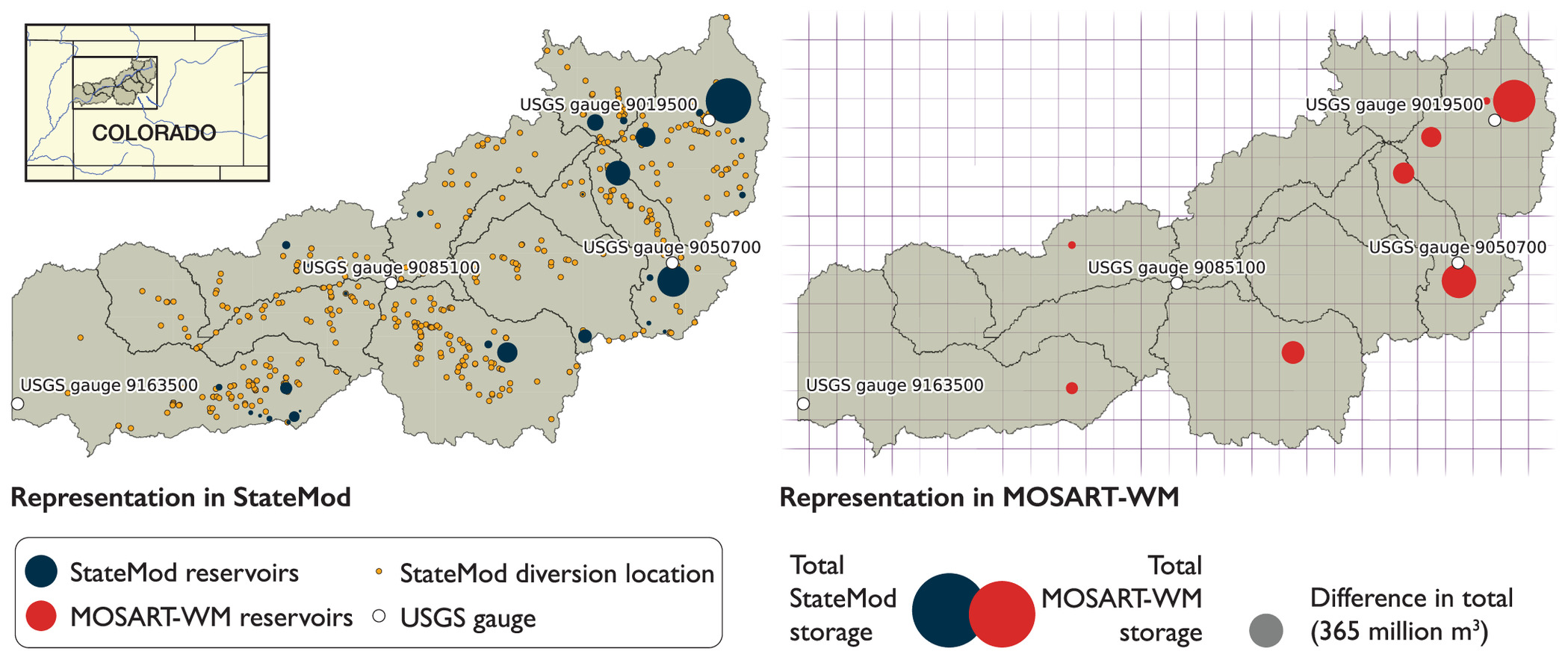
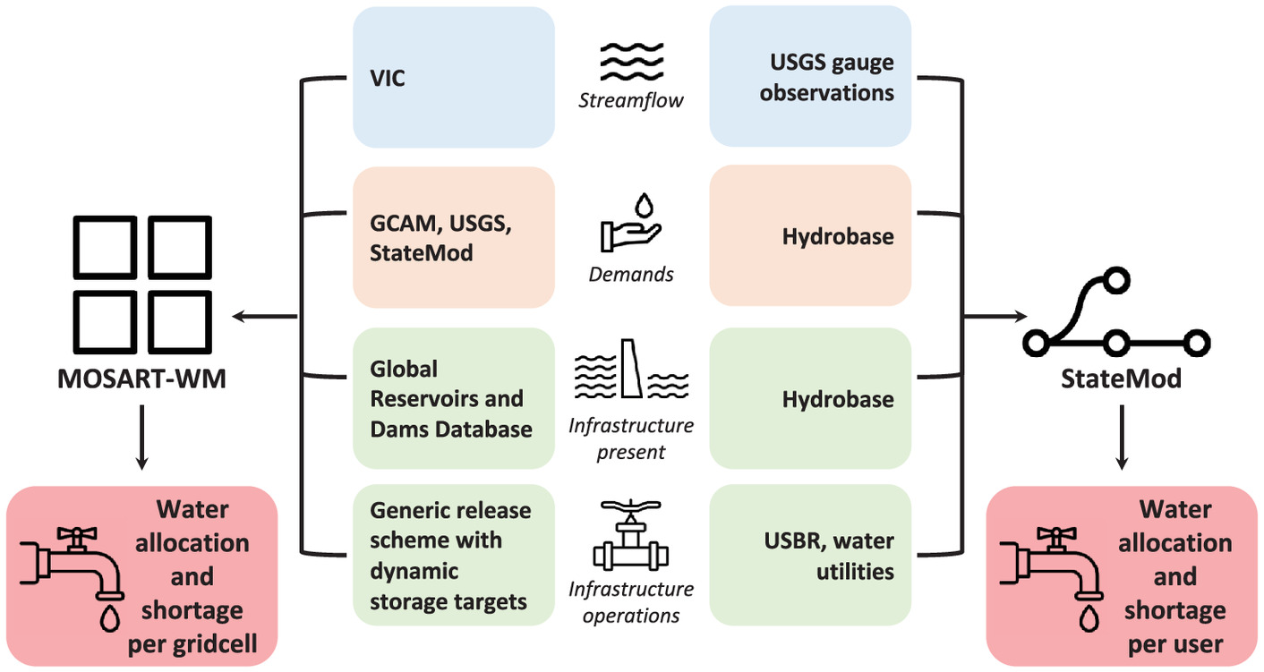
Our study focuses on the Upper Colorado River Basin (UCRB) within the state of Colorado. The basin spans (9,915 sq mi) in western Colorado and includes the headwaters of the Colorado River at the Continental Divide. Several thousand diversion locations draw water from the river and its tributaries, indicated by orange points in Fig. 1. Consumptive use in this basin is primarily for the purposes of irrigation, but major transbasin diversions of water also take place, delivering (460,000 acre-ft) of water per year to northern and eastern Colorado for municipal, industrial, and agricultural uses (State of Colorado 2015). Several of these diversions are accommodated by reservoirs, indicated by the dark blue points in Fig. 1. The subsequent sections present the two water management models used in this study, StateMod and MOSART-WM, with Table 2 presenting a summary of the differences in the representation of various system elements (e.g., demands, infrastructure, and operations) and Fig. 3 summarizing the differences in inputs and outputs.
| Feature | StateMod | MOSART-WM |
|---|---|---|
| Water availability | Naturalized inflows based on USGS measurements and diversion data. | Spatially distributed simulated runoff based on the hydrology model VIC informed with observed gridded climate. |
| Irrigation demands | Calculated for each crop using maximum irrigation water requirement and irrigation efficiency. | Simple crop water demand model that applies region-specific assumptions of blue (irrigation water) needs per crop and irrigation efficiencies. Crop areas are derived from GCAM simulations. |
| Municipal demands | Using monthly averages of recent records. | Assumed to be a function of population, per-capita income, and water prices. Coefficients are estimated by calibration to match historical estimates of municipal water use. |
| Industrial demands | Using monthly averages of recent records. | Includes water use for electricity generation, primary energy sector, and manufacturing. For each, technology-specific water use coefficients are applied to the various industrial activities. The industrial activity levels are the output of GCAM simulations. |
| Transbasin demands | Using utility records where available or set to historical average monthly diversions. | Not represented |
| Irrigation consumptive use | Calculated using crop information (e.g., type and irrigation efficiency). | Withdrawals demands are converted to consumptive demands for input into MOSART-WM by using estimated conversion factors. |
| All other consumptive use | Using constant rates. | Withdrawals demands are converted to consumptive demands for input into MOSART-WM by using conversion factors. |
| Reservoir operations | Defined rules to represent diversions to meet content targets and diversion projects. | Generic operating rules that mimic monthly release and storage variations patterns based on the objective of the reservoir (e.g., flood control, irrigation, and so on), its physical characteristics and inflow climatology, and follows daily constraints for minimum environmental flow, and minimum and maximum storage volumes. For example, large reservoirs operated for flood control will have their storage reduced prior to the flood freshet and scale to capture and control this flooding, whereas irrigation reservoirs will fill up their storage for sustained release throughout the irrigation season. |
| Prior appropriation water rights | Accounted for all important rights [above (11 cu ft/s)]. | Water rights are not represented. Rather, MOSART-WM incorporates a generic water allocation priority rule in which non-irrigation demands are first met followed by irrigation demands. Following this prioritization, reservoir water supplies are further distributed such as to distribute shortage proportionally among model cells. |
Sources: Data about the StateMod inputs and representation from CWCB and CDWR (2016). Data about MOSART-WM inputs and representation from Hejazi et al. (2013, 2015) and Voisin et al. (2013b).
Note: Information for MOSART-WM is representative of the default model (referred to as GCAM-informed MOSART-WM). For the other two runs included in this paper, water demands have been adjusted as described in the “Methods” section.
StateMod
StateMod is a network-based water system model for water accounting and allocation. StateMod determines water availability to individual users and projects based on hydrologic conditions, water rights, and operating rules (CWCB and CDWR 2016). StateMod is a component model of Colorado’s Decision Support System (CDSS), a collection of databases, data management tools, and models, used to support water resources planning in major water basins in the state, particularly those draining into the Upper Basin of the Colorado River: White, Yampa, Upper Colorado, Gunnison, Dolores, San Juan, and San Miguel (CWCB 2012; Malers et al. 2001; Parsons and Bennett 2006). CDSS and StateMod are distinguished in their use to adjudicate conflicts and allocations within the basins, which requires them to capture a high degree of specific users’ details. The implementation of StateMod for each basin represents a base streamflow data set that simulates current demands, infrastructure, and administrative environment to allow for the evaluation of potential future impacts of changes in diversions, reservoirs, water rights, or management strategies (CWCB and CDWR 2016). For each basin, StateMod replicates its unique application of the prior appropriation doctrine according to the basin’s hydrologic conditions and operational rules and agreements (Table 2).
The UCRB StateMod model is made up of more than 800 nodes, representing key diversion structures, reservoirs, and instream flow structures (CWCB and CDWR 2016). Because it would be impractical to represent each and every water right and diversion structure in this basin individually, a smaller number of key structures of a basin were identified so as to ensure a full accounting of the basin’s water balance and that all consequential operations are represented. Diversion structures with total absolute water rights equal to or above () were considered important and are explicitly represented in their strict locations. In total, there are 375 key diversion structures in the UCRB StateMod model making up 75% of the consumptive use of water in the basin (CWCB and CDWR 2016). The remaining consumptive use was modeled using aggregate diversion structures, with 65 nodes in the model.
StateMod explicitly represents reservoirs in the basin with decreed capacities equal to or in excess of (4,000 acre-ft). In this manner, 94% of the total storage capacity in the basin is explicitly modeled using 18 reservoir structures, whereas the remaining 6% of storage capacity is represented using 13 aggregated reservoir and stock pond structures (presented in blue dots in Fig. 1). StateMod models the storage capacity of this basin in its entirety, i.e., 1,811 million (1,468,038 acre-ft). Operations and storage targets for the key reservoirs are represented explicitly using the different rights (accounts) related to each operation or project (Table 2). The aggregated reservoirs are represented with one account and serve as supplemental supply to direct flow rights, with their operational targets being the respective unmet demand.
Water demands for irrigation, municipal, industrial, and transbasin uses are calculated using different procedures. For irrigation structures, monthly demand is calculated based on the maximum crop irrigation water requirement, divided by the average irrigation efficiency of each structure and its historical diversion during that month, which also ensures that irrigation requirements are anticorrelated with streamflow. This estimated demand represents the volume of water the diversion location would have diverted absent any physical or legal availability constraints. Monthly municipal and industrial demands are set to averages of recent records. Transbasin demands are set to values provided by the administering authorities where available. Otherwise, for transbasin demands going to municipal purposes, demands are set to historical average monthly diversions, and for those delivered for irrigation purposes, demands are set using wet, dry, and average patterns from historical diversion data.
To estimate consumptive use of water for irrigation uses, StateMod considers a monthly irrigation efficiency for each structure as well as its soil moisture capacity. Soil moisture capacity is modeled as a small reservoir, retiming the physical consumption of the water and affecting the amount of return flow in any given month. Soil moisture capacity for each irrigation structure is based on Natural Resources Conservation Service mapping. At each monthly time step, water that exceeds the crop water requirement and the capacity of the crop’s soil moisture returns to the stream. The timing of the return flows is determined using two patterns, one for diversions close to the stream and another for diversions taking place farther from the stream. Consumptive use for municipal diversions follows monthly efficiencies representing municipal consumptive use patterns. For industrial and hydroelectric power generation diversions, consumptive use is assumed to be 100% and 0%, respectively.
To appropriately simulate river basin operations, the model requires an estimate of undepleted naturalized flow. This calculation requires three steps (CWCB and CDWR 2016): (1) adjust flows in 78 USGS gauge locations by removing all historical operations and diversions with data provided by the US Bureau of Reclamation, local irrigation districts and water boards, and the State Engineer’s office; (2) for every gauge, fill in any missing data points in the time series using regression models with nearby gauges; and (3) distribute streamflow gains to any user-specified ungauged flow nodes necessary for the model’s operation. The resulting base streamflow data set used in this analysis assumes present day infrastructure, operations, and diversions superimposed on the naturalized flow.
MOSART-WM
MOSART-WM is a spatially distributed (i.e., grid-based) regional-scale river routing water management model consisting of a physically based river-routing base (MOSART) (Li et al. 2013) coupled with a generalized water-management (WM) submodel (Voisin et al. 2013b, 2017). In the river-routing component, simulated spatially distributed surface runoff is first routed across hillslopes and then discharged into a tributary subnetwork before entering the main channel to travel across grid cells. The water management component simulates reservoir storage and releases by adopting generic operating rules that mimic monthly release patterns based on the objective of the reservoir (e.g., flood control and irrigation), monthly inflow, storage levels, and water demand. These rules emulate typical reservoir operations simulations for specific uses (irrigation, flood control, and combinations) and are scaled to the reservoir characteristics and associated inflow and demand. More information on these generic operating rules has been given by Hanasaki et al. (2006), Nazemi and Wheater (2015a), and Voisin et al. (2013a). The daily operations further follow daily constraints for minimum environmental flow and minimum and maximum storage volumes. The water management component serves to allocate water supply to sector-specific water demands at the grid-cell resolution.
For input into MOSART-WM, we leveraged the large-scale hydrology simulations by Brekke et al. (2014) based on the macroscale physically-based variable infiltration capacity (VIC) hydrologic model (Liang et al. 1994) forced with observed historical climate (Maurer et al. 2002). The monthly spatially distributed (1/2 degree) sectoral consumptive water demand input to MOSART-WM was leveraged from Hejazi et al. (2015). The demand data set reflects the annual basin-scale emulation of sectoral water demand by a global climate assessment model that has been spatially and temporally disaggregated to a monthly and 1/2-degree resolution as described by Li et al. (2018). The historical emulations were calibrated regionally with respect to the USGS observations (Maupin et al. 2014) as evaluated by Hejazi et al. (2015).
The downscaling algorithms employed proxy information such as population and areas equipped with irrigation information to map water demands to a finer spatial scale of 1/2 degree. The monthly demand data set described in the preceding paragraph was further processed for input to MOSART-WM by disaggregating demand results from 1/2- to 1/8-degree resolution (the demand for each 1/2-degree grid cell was equally partitioned among the 1/8-degree cells it contains). The monthly demand was uniformly disaggregated to a daily time step for input into MOSART-WM. For our experiments, we used 2010 levels of sectoral water demands in order to isolate our results from the impact of global change, as done by Zhou et al. (2018).
In order keep the comparison of model elements to those strictly necessary to identify differences in our inferences, we eliminated the return flow transfer function from the MOSART-WM implementation used in this study, abstracting therefore water demand as only the demand for water to be consumed. Water demand was therefore input as a consumptive water requirement, and only consumptive water demands were extracted from the river channels. Because MOSART-WM dynamically simulates surface-water transport and availability, the demand for surface water was determined as the difference between the demand input and the amount provided by groundwater, as a preprocessing step. The demand was further specified to include both irrigation and nonirrigation (electricity, domestic, mining, livestock, and manufacturing) demands. Voisin et al. (2017) provided a more detailed description of the return flow and groundwater components. For the model experiments, we adjusted the baseline demand input for consistency with StateMod inputs (“Demand Harmonization” section).
The reservoir locations were obtained from the Global Reservoir and Dam Database (GRanD) reservoir database (Lehner et al. 2011). The GRanD database attempts to account for all surface water reservoirs with a storage capacity greater than , with many smaller dams and reservoirs being added where data become available. In MOSART-WM, only those reservoirs with storage capacity larger than are included to focus on reservoirs that most influence river discharge (Fig. 1). The reservoirs were mapped onto the stream network with aggregation of reservoir storage and reservoir-purpose (e.g., irrigation, flood control, and so on) assigned based on the reservoir with the largest storage capacity (Voisin et al. 2013a, b).
Water allocation in MOSART-WM involves a sequence of identifying various supply sources to meet water demand at individual grid cells (Fig. 2). The daily demand input for a grid cell is first met by extracting water from the water storage in the subsurface. The subsurface flow is then routed into the subbasin main channel. The remaining demand is then extracted from the main channel water storage, with the constraint to leave at least 50% of the flow in the main channel for computational stability in the hydrodynamic routing model. If the demand of a grid cell is still not fully met, the subbasin will request water from multiple reservoirs. A dependency database associates each grid cell with a reservoir, which can be used to request water. In order to maximize water supply, a grid cell within 50 km of a river can request water from all the reservoirs impounding this river and its tributaries as long as the elevation of the reservoir is higher than the grid cell. Biemans et al. (2011) provided more details on this dependency between grid cells and reservoirs, as well as a sensitivity analysis on the dependency relationships and their impact on simulated flow.
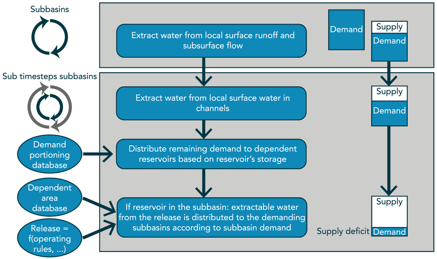
In our experiment, the demand from a grid cell to a specific reservoir equaled the remaining demand adjusted by the ratio of the storage in that reservoir to the combined storage of all reservoirs from which the grid cell can request water. This was determined at the beginning of each month in the simulation. As such, the grid cell request to one reservoir varied every month and every year. Conversely, the extractable water from the computed release from any given reservoir consisted of the release minus the minimum flow. That extractable water was distributed across the demanding grid cells specified by the dependency database with a priority for nonirrigation water demands first, followed by irrigation demands. If the available supply did not meet the demand to this reservoir, the available supply was distributed to the demanding grid cells proportionally to the ratio between the demand of each grid cell’s demand and the total demand to that reservoir. If the grid cell water demand to the surface water system was still not met, then this deficit was accounted as a shortage for that day. Voisin et al. (2017, 2013a) provided additional details on the dependency database, allocation scheme, and the reservoir release procedure used by WM.
Comparative Analysis Approach
The principal aim of this study is to compare the insights one would draw from the two models about water scarcity in the UCRB. In doing so, the largest barrier arises when comparing model elements (inputs, outputs, and processes) that are conceived and represented very differently by models of different classes. For example, due to the scales at which they operate, the models utilize different data sets with information about streamflow, human demands, infrastructure, and operations (Fig. 3). To account for human demands, standard MOSART-WM experiments utilize outputs from GCAM simulations, which significantly underrepresent basin demands as specified by the Department of Natural Resources in StateMod.
Adjusting MOSART-WM water demands to StateMod equivalents presents another complication. The implementation of MOSART-WM used in this experiment abstracts water demand as only being the demand for water to be consumed in order to eliminate the effects of return flows, as described previously. The abstraction used by StateMod also includes conveyance losses and nonconsumptive diversions (such as for power generation), so adjustments between the two need to take that into account.
The scale differences of the two models also complicate the comparison of their outputs. State variables, such as water shortages, are spatially distributed in MOSART-WM but represented in explicit node points in StateMod. Directly relating one to the other is not straightforward because one MOSART-WM grid cell (representing a spatial extent) is not equivalent to one StateMod node (representing one diversion location or other structure)—a grid cell can have several or no diversion locations within it. We therefore compared model outputs across scales using three system states: basinwide water balance, monthly streamflow, and threshold-based classifications of water shortage vulnerability.
For the current experiments, MOSART-WM was simulated at 1/8-degree spatial resolution on a daily time step across the continental United States for the historical period 1980–2008, with model results subsequently aggregated to a monthly resolution. Results for the Upper Colorado River basin were extracted from the model domain for comparison with StateMod output over 218 grid cells. Subsequent sections further describe the various external inputs into MOSART-WM, endogenous model processes, and model options, also summarized in Table 2. The following sections describe how the inputs were harmonized to enable the comparison and how the output comparison was performed across the three state variables.
Harmonizing Demand Inputs
For the comparative evaluation between StateMod and MOSART-WM, three different versions of MOSART-WM demand inputs were used to diagnose the degree to which demand differences influence the model comparison: (1) the integrated assessment model (GCAM) demand as specified by Voisin et al. (2013b) and described in the MOSART-WM model description given previously (referred to as GCAM-informed MOSART-WM), (2) downscaled USGS-based estimates of water demand based on Moore et al. (2015) (USGS-informed MOSART-WM), and (3) the same downscaled USGS-based estimates of water demand scaled such that the total basinwide consumptive water demand in MOSART-WM matches that defined in StateMod (StateMod-informed MOSART-WM).
Although calibrated with respect to regional USGS observed water demand, the GCAM version of demand is the output of a relatively coarse resolution global integrated assessment model that does not take local-scale water availability into account, with a subsequent downscaling process applied to define water demand at -degree resolution (Voisin et al. 2013b). The USGS-based estimates, in contrast, are based on actual historical estimates of water use developed at the county level, further spatially downscaled based on proxy information similar to the process applied to the GCAM model output. The GCAM and USGS estimates are fundamentally different because the former is the result of global economic model output whereas the latter is observationally derived. GCAM state-scale annual withdrawal water demand is, however, calibrated with respect to USGS for year 2010 [Hejazi et al. (2015) provided the evaluation].
Finally, we also tested a version in which we scaled the USGS demand to match StateMod inputs of demand at the basin-level, applying a uniform multiplier across all model cells in the basin. StateMod demands are based on detailed basin-level historical records and thus represent the most localized source of information available. This final version of demand allowed for a comparison between StateMod and MOSART-WM in which demand has been harmonized between the two models, allowing us to isolate nondemand model factors and their influence on differences between model outcomes.
Across each of the MOSART-WM demand versions described previously, water demand was specifically input into the model as consumptive rather than withdrawal demand. For the harmonization experiment in which we scaled the USGS-based demands to StateMod demands (StateMod-informed MOSART-WM), we applied the following sector-specific consumption/withdrawal conversion ratios following Hejazi et al. (2014b):
•
irrigation diversions: (41.5%);
•
municipal and industrial diversions: (13.9%);
•
reservoir diversions: 0 (0%);
•
transbasin diversions: 1 (100%); and
•
any other diversion: 0 (0%).
Evaluating Outputs
As explained previously, output comparison between the two models has been performed at various levels: the annual basinwide water balance, monthly streamflow at four gauges along the main stem of the river, and classification of water shortages. We next present how these comparisons were performed.
Basinwide Water Balance Comparison
The water balance comparison tracks three principal model outputs: total surface runoff in the basin, total annual demand, and end-of-year total storage at all of the basin’s reservoirs. Total surface runoff in MOSART-WM is estimated as the sum of the surface runoff input to all grid cells representing the basin (input hydrologic simulations). Input surface runoff is the same across all three MOSART-WM runs. Total surface runoff in StateMod is calculated by summing all water gains at all inflow nodes. StateMod considers as total inflow to the basin (i.e., water available for allocation depending on institutional and physical constraints) the sum of runoff, return flows, and positive changes in reservoir and soil moisture contents, with the sum of runoff and return flows making up over 99% of total inflows.
Water demands in StateMod represent the amount a given structure would have diverted absent physical or legal availability constraints. At every time step, StateMod determines allocative diversion at each location as the minimum of (1) its water rights, (2) the available supply of water in the stream, (3) its diversion capacity, and (4) the water demand. Total water demand in StateMod is therefore always equal to or greater than the diversions that take place. The allocated diversions are then used to meet the structure’s demand and return flows from each structure are estimated as the difference between demand and consumption. In this experiment, MOSART-WM represented water demands only as consumptive (as explained previously), and total water demands were estimated as the sum of all demands in every grid cell in the basin. Finally, storage levels in the basin were calculated for both models as the sum of all reservoir volume at the end of December each year.
Monthly Streamflow at Four Gauges
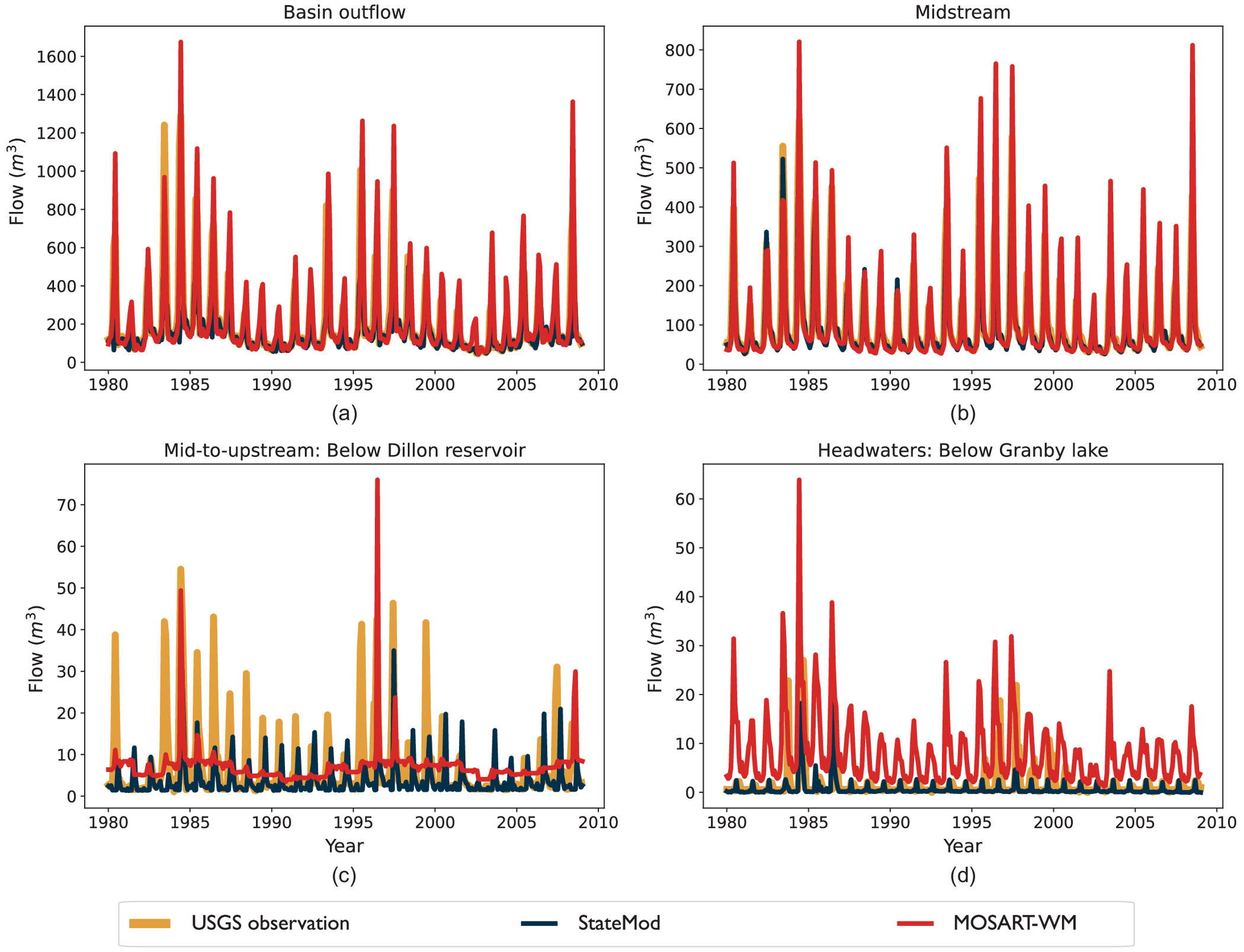
We also compared the streamflow represented by each model against USGS observations at four gauges in the basin (Fig. 1). The four locations were selected to track how streamflow estimates compare with observations, moving from the basin outlet to the headwaters. The four gauge locations were the following: basin outlet near the Colorado–Utah state line (USGS gauge 9163500), midstream of the Colorado River below Glenwood Springs, Colorado (USGS gauge 9085100), on the Blue River tributary below the Dillon reservoir (USGS gauge 9050700), and at the headwaters of the Colorado River near Granby, Colorado (USGS gauge 9019500). For the StateMod-modeled flows, data were extracted at the nodes representing those USGS gauges in the network representation used by the model. For MOSART-WM flows, we used the streamflow at the grid cell containing the main river channel and nearest to the latitude and longitude of each of the gauges.
Classification of Water Shortage Vulnerability
Evaluating water scarcity vulnerability for basins with a large number of stakeholders requires the use of metrics that are relevant to the decision makers and address concerns of credibility, salience, and legitimacy (White et al. 2010). Given the variability of hydrologic conditions, these metrics also need to account for temporal variations in vulnerability (for example, a decade of wet conditions where supply is well met followed by 5 years of drought). In this study, we focused on water shortages (unmet demands) experienced by basin users as an indicator of water scarcity vulnerability, by estimating their magnitude (as a percentage of demand), their frequency of annual occurrence, and their annual duration. Because water resources management is typically concerned with ensuring the necessary volumes of water across different needs, it is common to establish minimum or maximum levels of performance and use them to gauge whether system or user vulnerability is acceptable and identify policies to pursue (Beh et al. 2017; Hall and Borgomeo 2013; McPhail et al. 2018).
In multiactor systems, such as the UCRB, using a single metric, either applied uniformly across all users in the basin or applied on aggregate to the entire basin, ignores the users’ potential asymmetries in capacity and agency to adapt to change (Hadjimichael et al. 2020). This is especially the case in systems where users span small agricultural producers, large agricultural cooperatives, industrial producers, and municipal suppliers. Further, because the aim of the study was to assess the consistency of water scarcity vulnerability inferences between two models, the choice of a single metric by which such assessment is made might bias the comparison.
We therefore employed two types of water shortage metrics, each comprising combinations of magnitude, frequency, and duration levels. The first metric creates bins between 0% and 100% for both the magnitude percentage of shortage (as it relates to demand) and its frequency of occurrence (percent of years in the simulated record). We considered 10 bins of 10% increments for the magnitude dimension and 20 bins of 5% increments for the frequency dimension. Combining these bins created 200 possible magnitude and frequency combinations that can be used as a water shortage vulnerability metric. The second metric replicates this procedure, but instead of looking at a frequency of occurrence of a particular level of shortage, tracks its duration in increments of continuous years, up to a maximum of 30 years. This generated 300 possible magnitude and duration metric combinations. Applying all metrics allowed us to compare the consistency of inferences drawn from the two models across a number of thresholds in order to minimize comparison bias and ensure the relevancy of the inferences that are being assessed.
Results
Due to the differences in scale and structure between the two models as well as their state variables, the comparison of inferences about water scarcity drawn from the two was performed across several scales (basinwide, upstream to downstream gauges, individual, and grouped shortages), several state variables (streamflow, storage, and water shortages), and several water shortage metrics (500 combinations of magnitude, frequency, and duration). Three instances of MOSART-WM were simulated, namely GCAM-informed, USGS-informed, and StateMod-informed, each referring to the respective data set informing the water demands used as input. We used all three instances for the basinwide comparison but only focused on the StateMod-informed MOSART-WM run for subsequent comparisons of monthly streamflow and shortages because it eliminated the demand discrepancy between the two models, as can be seen in Fig. 4(b) and discussed subsequently.
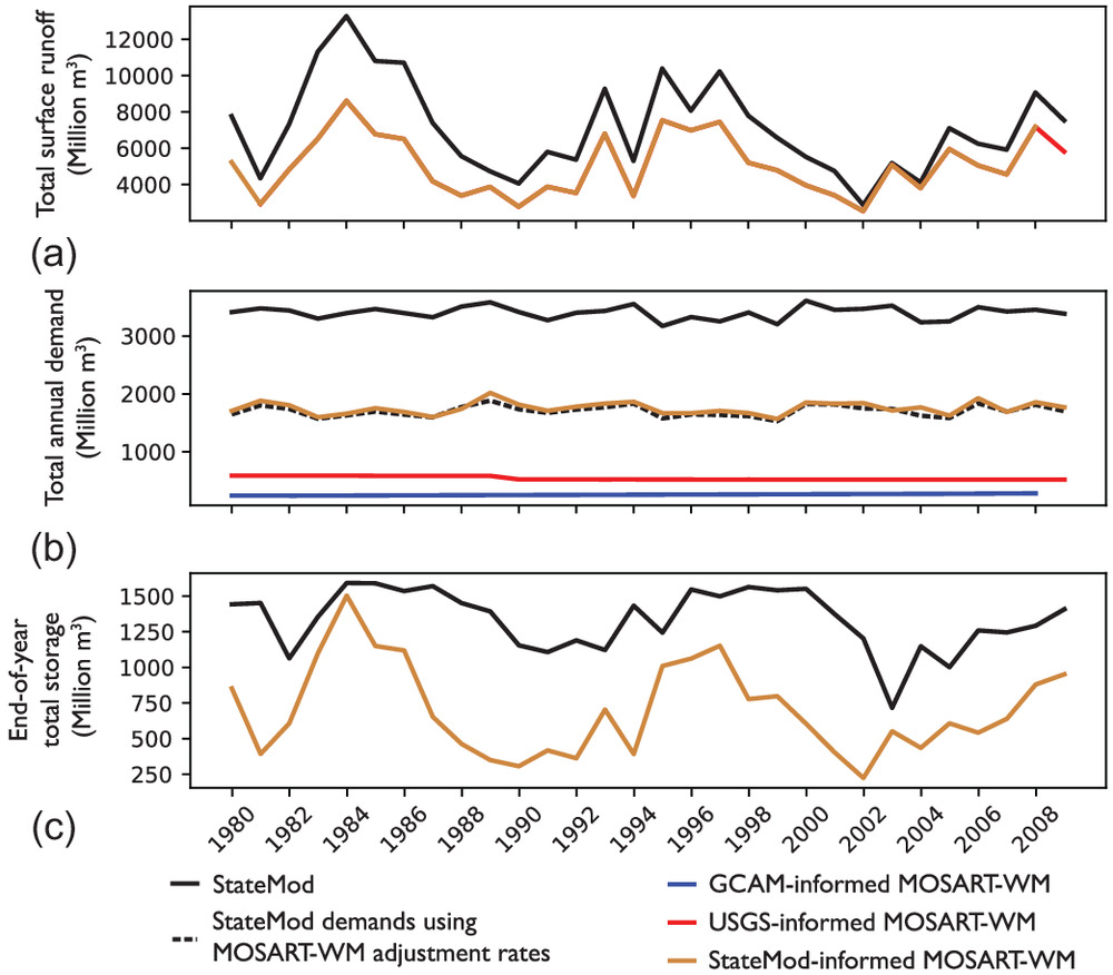
Inferences drawn from the two models are first compared at the basin scale, presented in Fig. 4. Total surface runoff [Fig. 4(a)] was the same across all three MOSART-WM runs because it is an input to the model, indicated by the brown line. Total surface runoff in StateMod is indicated in black and represents the sum of runoff and return flows. Surface runoff inputs to MOSART-WM were obtained through large-scale hydrologic simulations by Brekke et al. (2014) using the macroscale VIC model. Total surface runoff in MOSART-WM does not include return flows in these runs because only the consumptive parts of demand are diverted from the surface flow. The MOSART-WM surface runoff input from VIC appears to underestimate total surface runoff in this basin [Fig. 4(a)], especially during wetter periods (e.g., 1982–1988). This difference is attributed directly to the VIC model used to produce this runoff input. The Brekke et al. (2014) evaluation was conducted at a downstream location for a larger drainage area and has not been calibrated to this scale. Both models capture the occurrence of dry periods in the region (e.g., 1988–1992 and 2002–2006), as noted in the literature (Pielke et al. 2005; Rhee et al. 2018).
Different total annual demands inform the two models [Fig. 4(b)]. StateMod represents water demands as the ideal amount the user or structure would have diverted absent physical or legal availability constraints, as described in previous sections. Depending on the available flow and the users’ right seniority, only part of the water demands is allocated to users, resulting in shortages to users throughout the basin. Out of the total allocated volume of water across the basin, approximately 20% is consumed on average every year, with the rest being returned to the stream at variable rates depending on type of water use and its location.
Water demands in MOSART-WM represent only consumptive use demands, in other words, only the consumptive component of what is allocated (which is, by definition, lower than the ideal water demands used for accounting by the state and its models). To allow direct comparison between the StateMod water demands and the consumptive water demands used by MOSART-WM, we used withdrawal-to-consumption ratios for each type of use, as explained in previous sections. The resulting conversion is shown in Fig. 4(b) as a dashed line. Be that as it may, the original MOSART-WM (line in blue), which uses downscaled water demand forcings from GCAM, as well as the adapted version of MOSART-WM, which uses adjusted water demand data from USGS (line in red), both underrepresent these demands for consumptive use: the GCAM-informed demands and the USGS-informed demands are approximately 10% and 25% of the StateMod-informed demands, respectively [Fig. 4(b)].
Lastly, Fig. 4(c) compares the total end-of-year (December) stored volume of water across the basin, as represented by the two models. All instances of MOSART-WM (GCAM-, USGS-, and StateMod-informed) had the same storage values because most of the represented demand is downstream of the reservoirs and reservoir operations are essentially driven by monthly inflow climatology. Total stored volume was underrepresented by MOSART-WM, largely due to the underrepresentation of available storage in the basin (Fig. 1). StateMod represented the entire storage capacity in the basin, at 1,811 million . In StateMod and with the Colorado State institutional structure, reservoir storage is specifically managed to meet the demand. Approximately 75% of the reservoir capacity was used at varying levels during the 1980–2009 period, dropping to around 40% at the end of 2003 (year after the driest). MOSART-WM represents a smaller storage capacity in this basin, 1,446 million , because the reservoirs represented in the GRanD database have a minimum cutoff of storage capacity being greater than (Lehner et al. 2011). This capacity was also used at lower levels: stored water in the basin was represented at approximately 49% of the available storage, with the lowest level reaching 16% of total capacity in 2002. Fig. S1 presents the same results, but with the fraction of reservoir storage in each model instead of their absolute volumes. It is worth noting that the two models start with different storage levels, which also vary much more substantially in the MOSART-WM simulation (coefficient of variation for StateMod reservoir levels is 15.8%, and for MOSART-WM it is 45.3%).
With regards to streamflow, the two models are compared against USGS observations at four gauges in the basin (Figs. 5 and S2 ). At the basin outflow and the midstream location [Figs. 5(a and b)], both models tracked the observed flow time series fairly closely. At the gauge below Dillon reservoir, on the Blue River tributary, MOSART-WM appears to underestimate high flows and overestimate low flows [Fig. 5(c)]. Because this gauge is located below the Dillon reservoir, the low-flow discrepancy could be attributed to reservoir releases not represented in the model during those periods. The last gauge is located in the headwaters of the river, below Granby Lake [Fig. 5(d)], where both models diverge from observations—this is seen more notably when comparing flow duration curves [Fig. S2(d) ]. This is partly because both models were calibrated starting from the basin outflow and struggled to match observations closer to the headwaters. Another potentially contributing factor here is the fact that this USGS gauge lacked streamflow measurements from October until April for most of the comparison period. To allow a comparison here, we used average monthly observation values from months in the record that were available, as calculated during the StateMod calibration process (CWCB and CDWR 2016). It is also worth noting here that the water demands used in the MOSART-WM simulations (i.e., GCAM-, USGS-, or StateMod-informed) did not affect the simulated streamflow presented.
To understand the effects of the discrepancies between the two models on the inferences one would draw about water scarcity in this basin, we looked at water shortages estimated by the two models. For StateMod, shortages were estimated at each model node, each of which represents a diversion location or a small group of them. In MOSART-WM, shortages were estimated at model grid cells (representing a spatial subsection of the basin). To limit the potential bias introduced by the choice of water scarcity metric as well as ensure their relevance across decision makers and stakeholders in such a multiactor basin, we used two types of metrics: (1) one focused on combinations of shortage magnitude (percentage of demand) and frequency (percentage of time), and (2) the second focusing on shortage magnitude (percentage of demand) and duration (number of continuous years), as detailed in the “Methods” section. Fig. 6 presents the resulting vulnerability classification of users in this basin, with Figs. 6(a and b) showing classified nodes using StateMod outputs and Figs. 6(c and d) showing classified grid cells using MOSART-WM outputs.
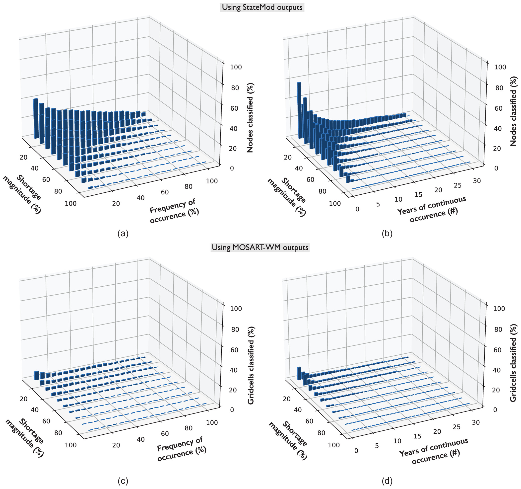
Fig. 6(a) shows the percentage of StateMod nodes that would be classified as vulnerable under the different combinations of magnitude and frequency levels. For example, if we choose as our metric that a user is vulnerable to water scarcity if they experience a water shortage of 10% of their demand 5% of the time (i.e., the column in the back left corner of the flat plane) then 41% of them would be classified as vulnerable. The remaining 59% of users experience shortage levels that are either smaller in magnitude or less frequent, or no shortages at all, under the conditions present during the 1980–2009 period. Because this is the strictest metric combination considered (acceptable levels of magnitude and frequency are the lowest), it follows that this is also the maximum percentage of users that would be classified as being vulnerable under any of the remaining magnitude and frequency combinations.
Alternatively, as an illustrative example for the metric considering combinations of shortage and duration [Fig. 6(b)], a user is vulnerable to water scarcity if they experience a water shortage of 10% of their demand for 5 consecutive years (i.e., the fifth from the left column in the back of the flat plane) yielding the classification of 22% of the users as being vulnerable. Under any combination of shortage-duration metrics, the largest number of users that would be classified as vulnerable to water scarcity is 58%. Lastly, in Figs. 6(a and b), there is always a small number of users that experience at least some level of shortage (columns in the back right corners of both panels).
The implication of these StateMod results is that even with the strictest metric combinations considered, approximately half of the basin would not be identified as vulnerable to water scarcity during this period. As a result, even with the fine-grained outputs of StateMod, if one were to aggregate to a basinwide metric by combining all demands and shortages across users, the shortages that were experienced would be dampened by the ones that did not. Specifically, within the studied period, the basin as a whole experienced a total shortage of 10% of its total demands 3.4% of the time for no more than 1 year in duration. In other words, none of the metrics shown in Figs. 6(a and b) would classify the entire basin as vulnerable to water scarcity even though up to 58% of its users would be.
It is also worth noting that this analysis used a short period of recent historical conditions with little hydroclimatic variability and assumed stationarity because the primary aim has been to investigate how inferences from the two models converge. Under more realistic conditions of change, the presence of increased variance in the states of the system (i.e., hydroclimatic factors such as streamflow and water demands) as well as in their spatial distributions could significantly increase this difference between user-level experience and the attenuated basin-level conclusion (Hadjimichael et al. 2020; Hyun et al. 2019).
Figs. 6(c and d) suggest that a similar type of attenuation is occurring with the MOSART-WM outputs. Model outputs in this case were classified using the MOSART-WM grid cells that overlap the basin (Fig. 1) and the water shortage assigned to each grid cell by the model was used to identify how many grid cells would be considered vulnerable using the same metrics as described previously. Looking at the magnitude-frequency metrics [Fig. 6(c)], the largest percentage of grid cells that would be classified as vulnerable under the metric instance of a water shortage of 10% of their demand 5% of the time is approximately 9%. Looking at the equivalent strictest metric in magnitude-duration spectrum [Fig. 6(d)] for the case where a water shortage of 10% of demand for 1 year yields a classification of 13% of basin grid cells as being vulnerable. Using MOSART-WM to evaluate water scarcity vulnerability for this basin produces a different picture, one where the majority of the basin is not vulnerable.
Another interesting insight is that a basinwide aggregation of all grid cells would lead to conclusions that are more consistent with the grid cell–level than the equivalent StateMod comparison described previously. Specifically, aggregating demands and shortages across all grid cells would indicate that the basin as a whole experienced a 10% shortage 73% of the time during the studied period, with 11 consecutive years as its maximum duration. These results suggest that MOSART-WM estimates larger and longer shortages on average, but the variance of these shortages is much smaller. Conversely, StateMod estimates smaller and shorter shortages on average, but represents much larger variability among the basin users.
This could be due to the fact that MOSART-WM does not explicitly represent the allocation and other institutional mechanisms that define how much and to whom water is diverted in the basin. Instead, the model adopts an allocative approach that focuses on a spatially distributed water balance accounting of basin inflows and outflows through time and attempts to equalize shortage across cells (for any number of cells connected to upstream reservoirs, the reservoirs will proportion available water supply to the unmet demand of each cell). The spatially distributed nature of this accounting can also attenuate imbalances between shortages and demands, as basin users are not distributed equally across all grid cells of the basin. If the majority of diversions takes place in a small number of MOSART-WM grid cells, estimating the percentage of grid cells that is short on water biases our inferences about how much of the basin is vulnerable.
With regards to the spatial consistency of these shortages, Fig. 7 focuses on three water districts in the basin and compares the total shortages across all StateMod nodes present in each district with the total shortages across all MOSART-WM grid cells overlapping each district. Fig. 7(a) shows the location and extent of these districts in the basin. In Figs. 7(b–d), the solid lines indicate the sum of all monthly shortages across all StateMod nodes and brown lines indicate the sum of all monthly shortages across all MOSART-WM grid cells.
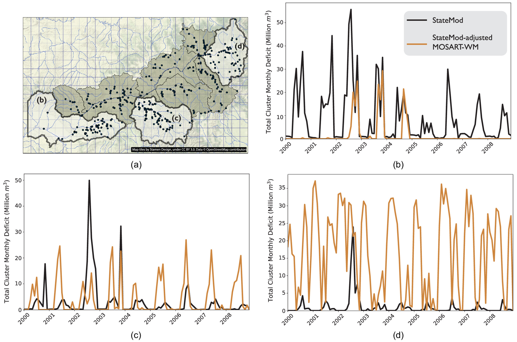
For the water district nearest the basin outflow [Fig. 7(b)], MOSART-WM assigns no shortages () for most of the 9-year period, with the exception of years 2002–2004. For the midstream water district [Fig. 7(c)], MOSART-WM appears to underestimate shortages assigned by StateMod during the most severe year (2002) and overestimate shortages during all others. Lastly, in the uppermost water district [Fig. 7(d)], MOSART-WM consistently overestimates shortages across all years in the selected period. These findings can be attributed to the allocative mechanisms used by MOSART-WM and other LHMs to proportion reservoir water supply to dependent cells downstream from them (Nazemi and Wheater 2015b).
Conclusion
Large-scale hydrologic models and basin-scale water systems models are being developed by their respective communities to study water supply availability and shortage from two different vantage points: the former emphasize sound representation of regional and global hydroclimatic processes, the latter prioritize human water management and use. This study explored whether representative models from the two communities, MOSART-WM and StateMod, are indeed consistent in the insights they produce regarding water scarcity in a basin, and whether insights from one can be used to best inform the other. The two models differ in scale and structure, so the comparison of inferences was performed across several levels of aggregation (basinwide, upstream to downstream, individual, and group shortages), state variables (streamflow, storage, and water shortages), and water shortage metrics (500 combinations of magnitude, frequency, and duration).
Our findings showed that both models captured the aggregate monthly effects of all water management processes in the basin fairly well, with the basin outflow [Fig. 5(a)] represented closely by the two models. This suggests that besides providing a regionally consistent model of hydrologic and other processes, the large-scale model can in fact be used to bridge aggregate dynamics between interacting basins for which high-resolution models might not exist. From the perspective of the water systems modeling community, this capacity could, for instance, allow for analyses on how changes in an upstream basin (for which a high-resolution model is not available) affect a basin of interest. Drawing water availability and vulnerability conclusions for smaller areas within the catchment however becomes a limitation for the large-scale model. Even though midstream streamflow dynamics were captured fairly well [Fig. 5(b)], when moving upstream [Fig. 5(c)] MOSART-WM begins to diverge from observations and StateMod, especially in the headwaters, where both models struggled due to the accuracy of inflow data. This results in different conclusions being potentially derived about water scarcity vulnerability for water users in this basin.
To compare these inferences, we used a set of water shortage metrics (Fig. 6) that classified whether model nodes (StateMod) or model grid cells (MOSART-WM) would be considered vulnerable during this 30-year period. The comparison suggested that looking at the basin as a whole (i.e., all aggregated shortages as a percentage of all aggregated demands), MOSART-WM estimated larger and longer shortages than StateMod. When looking at the variance across grid cells and nodes, respectively, we observed much larger variability among the basin users described by StateMod. This is attributed to main differences in the two models: the lack of detailed allocation and operation processes that describe how prior appropriation in the basin consistently allocates available water to senior users first, and the spatially distributed nature of MOSART-WM, which evenly allocates available water to sets of users associated with specific reservoirs.
Due to this spatial distribution, individual grid cells in this model should not be assessed in isolation. Our vulnerability classification in Fig. 6 attempted to overcome this by looking at the percentage of all grid cells in the basin meeting a vulnerability criterion, but alternative aggregate mappings or thresholds might be more appropriate when attempting to actually inform the operation of the large-scale model based on outputs from the basin-scale model. We therefore complemented our assessment with a comparison using three water districts in the basin (Fig. 7). Looking at the aggregate shortage of the grid cells present in each district compared with the aggregate shortage of the nodes present clarified how the subbasin performance of MOSART-WM is in fact very different from StateMod. Water shortages were significantly underestimated in one district [Fig. 7(b)] and significantly overestimated in another [Fig. 7(d)]. This explains why even though on aggregate, the large-scale model appears to represent regulated flow fairly well, it still fails to capture the water scarcity variability within the basin.
This inconsistency also presents itself as a clear opportunity for how high-resolution basin-scale models can inform the modeling of human processes in regional or larger scales. Our results suggest that LHMs can be limited in how they assess the effects of conservation policies and other human interventions at the river basin scale. LHMs typically do not represent local hydrological conditions, water infrastructure, and water institutions that can be fundamental in shaping water shortages. In fact, MOSART-WM is the only model in its class that attempts to track water shortages, which is what allows for such a comparison to be performed. Other large-scale models, such as IAMs, typically do not represent water shortages. There is therefore an urgent need to better incorporate local water shortage processes and mechanisms in large-scale modeling approaches. Incorporating basin-scale information in large-scale models would enable not only a more nuanced representation of how water scarcity vulnerability manifests itself in a basin, but also the potential consideration of sensible human action feedbacks (i.e., how humans might respond to water shortages is different when their drought experience is more or less severe).
Incorporating more of this information is not an easy task however. The UCRB used in this example is a comparatively data- and model-rich basin, with a long history of data collection, management, and incorporation into model-based decision making. Extending the approach to much larger scales, such as those typically assessed by MOSART-WM, will require the use of agent-based models to emulate institutional and economic drivers of demand and supply allocation, data assimilation, and other machine learning methods to compensate for where observation data are sparse (Berglund 2015; Wada et al. 2017). Further, updating large-scale information with more accurate localized estimates (such as our adjustment of water demands) gives rise to complications in the large-scale model outside the basin under study because these estimates are no longer consistent with their original source—recall that the original version of MOSART-WM used water demands from GCAM, which were estimated at about 10% of the local values.
Future steps of this work thus include an examination of the implications of such adjustments to regions within the large-scale model, especially with regard to water deliveries and availability in basins downstream. Reconciliation of differences and coordinated development between LHMs and local water systems models offers the potential for improved water scarcity analysis that accounts for both large-scale dynamics (hydroclimate, regional markets, and so on) and detailed representations of the physical and institutional mechanisms that shape water scarcity at the local level.
Supplemental Materials
File (supplemental materials_jwrmd5_wreng-5522.hadjimichael.pdf)
- Download
- 457.72 KB
Data Availability Statement
All data and code to replicate the results of this study can be found in a repository online at https://github.com/antonia-had/Hadjimichael-etal_2021_JWRPM.
Reproducible Results
Md. Atif Ibne Haidar (reproducibility reviewer) downloaded all materials and reproduced results in all figures and tables.
Acknowledgments
This research was sponsored by the DOE Office of Science as a part of the research in MultiSector Dynamics within the Earth and Environmental System Modeling program.
References
Alcamo, J., P. Döll, T. Henrichs, F. Kaspar, B. Lehner, T. Rösch, and S. Siebert. 2003. “Development and testing of the WaterGAP 2 global model of water use and availability.” Hydrol. Sci. J. 48 (3): 317–337. https://doi.org/10.1623/hysj.48.3.317.45290.
Arnold, J. G., R. Srinivasan, R. S. Muttiah, and J. R. Williams. 1998. “Large area hydrologic modeling and assessment part I: Model development1. JAWRA.” J. Am. Water Resour. Assoc. 34 (1): 73–89. https://doi.org/10.1111/j.1752-1688.1998.tb05961.x.
Barrow, C. J. 1998. “River basin development planning and management: A critical review.” World Dev. 26 (1): 171–186. https://doi.org/10.1016/S0305-750X(97)10017-1.
Beh, E. H., F. Zheng, G. C. Dandy, H. R. Maier, and Z. Kapelan. 2017. “Robust optimization of water infrastructure planning under deep uncertainty using metamodels.” Environ. Modell. Software 93 (Jul): 92–105. https://doi.org/10.1016/j.envsoft.2017.03.013.
Berglund, E. Z. 2015. “Using agent-based modeling for water resources planning and management.” J. Water Resour. Plann. Manage. 141 (11): 04015025. https://doi.org/10.1061/(ASCE)WR.1943-5452.0000544.
Biemans, H., I. Haddeland, P. Kabat, F. Ludwig, R. W. A. Hutjes, J. Heinke, W. Bloh, and D. Gerten. 2011. “Impact of reservoirs on river discharge and irrigation water supply during the 20th century.” Water Resour. Res. 47 (3): W03509. https://doi.org/10.1029/2009WR008929.
Brekke, L., A. W. Wood, and T. Pruitt. 2014. Downscaled CMIP3 and CMIP5 hydrology prodictions: Release of hydrology projections, comparison with preceding information and summary of user needs. Washington, DC: Bureau of Reclamation.
Brown, C. M., J. R. Lund, X. Cai, P. M. Reed, E. A. Zagona, A. Ostfeld, J. Hall, G. W. Characklis, W. Yu, and L. Brekke. 2015. “The future of water resources systems analysis: Toward a scientific framework for sustainable water management.” Water Resour. Res. 51 (8): 6110–6124. https://doi.org/10.1002/2015WR017114.
Burrow, A., A. S. Hering, D. P. Morton, and A. M. Newman. 2021. “Optimal design and operation of river basin storage under hydroclimatic uncertainty.” J. Water Resour. Plann. Manage. 147 (9): 04021055. https://doi.org/10.1061/(ASCE)WR.1943-5452.0001337.
Calvin, K., and B. Bond-Lamberty. 2018. “Integrated human-earth system modeling—State of the science and future directions.” Environ. Res. Lett. 13 (6): 063006. https://doi.org/10.1088/1748-9326/aac642.
Condon, L. E., and R. M. Maxwell. 2014. “Feedbacks between managed irrigation and water availability: Diagnosing temporal and spatial patterns using an integrated hydrologic model.” Water Resour. Res. 50 (3): 2600–2616. https://doi.org/10.1002/2013WR014868.
CWCB and CDWR (Colorado Water Conservation Board and Colorado Division of Water Resources). 2016. Upper Colorado River Basin water resources planning model user’s manual. Denver: Colorado Water Conservation Board and Colorado Division of Water Resources.
CWCB (Colorado Water Conservation Board). 2012. Colorado River water availability study phase I report. Denver: Colorado Water Conservation Board.
Dang, T. D., D. T. Vu, A. F. M. K. Chowdhury, and S. Galelli. 2020. “A software package for the representation and optimization of water reservoir operations in the VIC hydrologic model.” Environ. Modell. Software 126 (Apr): 104673. https://doi.org/10.1016/j.envsoft.2020.104673.
de Boer, T., H. Paltan, T. Sternberg, and K. Wheeler. 2021. “Evaluating vulnerability of Central Asian water resources under uncertain climate and development conditions: The case of the Ili-Balkhash Basin.” Water 13 (5): 615. https://doi.org/10.3390/w13050615.
Dobson, B., G. Coxon, J. Freer, H. Gavin, M. Mortazavi-Naeini, and J. W. Hall. 2020. “The Spatial Dynamics of Droughts and Water Scarcity in England and Wales.” Water Resour. Res. 56 (9): e2020WR027187. https://doi.org/10.1029/2020WR027187.
Dolan, F., J. Lamontagne, R. Link, M. Hejazi, P. Reed, and J. Edmonds. 2021. “Evaluating the economic impact of water scarcity in a changing world.” Nat. Commun. 12 (1): 1915. https://doi.org/10.1038/s41467-021-22194-0.
Draper, A. J., A. Munévar, S. K. Arora, E. Reyes, N. L. Parker, F. I. Chung, and L. E. Peterson. 2004. “CalSim: Generalized model for reservoir system analysis.” J. Water Resour. Plann. Manage. 130 (6): 480–489. https://doi.org/10.1061/(ASCE)0733-9496(2004)130:6(480).
Fereidoon, M., and M. Koch. 2018. “SWAT-MODSIM-PSO optimization of multi-crop planning in the Karkheh River Basin, Iran, under the impacts of climate change.” Sci. Total Environ. 630 (Jul): 502–516. https://doi.org/10.1016/j.scitotenv.2018.02.234.
Flato, G. M. 2011. “Earth system models: An overview.” Wiley Interdiscip. Rev. Clim. Change 2 (6): 783–800. https://doi.org/10.1002/wcc.148.
Gleick, P. H. 2000. “A look at twenty-first century water resources development.” Water Int. 25 (1): 127–138. https://doi.org/10.1080/02508060008686804.
Graham, N. T., M. I. Hejazi, S. H. Kim, E. G. R. Davies, J. A. Edmonds, and F. Miralles-Wilhelm. 2020. “Future changes in the trading of virtual water.” Nat. Commun. 11 (1): 3632. https://doi.org/10.1038/s41467-020-17400-4.
Haddeland, I., et al. 2014. “Global water resources affected by human interventions and climate change.” Proc. Natl. Acad. Sci. U.S.A. 111 (9): 3251–3256. https://doi.org/10.1073/pnas.1222475110.
Haddeland, I., D. P. Lettenmaier, and T. Skaugen. 2006a. “Effects of irrigation on the water and energy balances of the Colorado and Mekong River Basins.” J. Hydrol. 324 (1–4): 210–223. https://doi.org/10.1016/j.jhydrol.2005.09.028.
Haddeland, I., T. Skaugen, and D. P. Lettenmaier. 2006b. “Anthropogenic impacts on continental surface water fluxes.” Geophys. Res. Lett. 33 (8): L08406. https://doi.org/10.1029/2006GL026047.
Hadjimichael, A., J. Quinn, E. Wilson, P. Reed, L. Basdekas, D. Yates, and M. Garrison. 2020. “Defining robustness, vulnerabilities, and consequential scenarios for diverse stakeholder interests in institutionally complex river basins.” Earths Future 8 (7): e2020EF001503. https://doi.org/10.1029/2020EF001503.
Hall, J., and E. Borgomeo. 2013. “Risk-based principles for defining and managing water security.” Philos. Trans. R. Soc. London, Ser. A 371 (2002): 20120407. https://doi.org/10.1098/rsta.2012.0407.
Hanasaki, N., S. Kanae, and T. Oki. 2006. “A reservoir operation scheme for global river routing models.” J. Hydrol. 327 (1–2): 22–41. https://doi.org/10.1016/j.jhydrol.2005.11.011.
Hanasaki, N., S. Kanae, T. Oki, K. Masuda, K. Motoya, N. Shirakawa, Y. Shen, and K. Tanaka. 2008. “An integrated model for the assessment of global water resources–Part 1: Model description and input meteorological forcing.” Hydrol. Earth Syst. Sci. 12 (4): 1007–1025. https://doi.org/10.5194/hess-12-1007-2008.
Hejazi, M., et al. 2014b. “Long-term global water projections using six socioeconomic scenarios in an integrated assessment modeling framework.” Technol. Forecast. Soc. Change 81 (Jan): 205–226. https://doi.org/10.1016/j.techfore.2013.05.006.
Hejazi, M., J. Edmonds, V. Chaturvedi, E. Davies, and J. Eom. 2013. “Scenarios of global municipal water-use demand projections over the 21st century.” Hydrol. Sci. J. 58 (3): 519–538. https://doi.org/10.1080/02626667.2013.772301.
Hejazi, M., J. Edmonds, L. Clarke, P. Kyle, E. Davies, V. Chaturvedi, M. Wise, P. Patel, J. Eom, and K. Calvin. 2014a. “Integrated assessment of global water scarcity over the 21st century under multiple climate change mitigation policies.” Hydrol. Earth Syst. Sci. 18 (8): 2859–2883. https://doi.org/10.5194/hess-18-2859-2014.
Hejazi, M. I., et al. 2015. “21st century United States emissions mitigation could increase water stress more than the climate change it is mitigating.” Proc. Natl. Acad. Sci. U.S.A. 112 (34): 10635–10640. https://doi.org/10.1073/pnas.1421675112.
Hyun, J.-Y., S.-Y. Huang, Y.-C. E. Yang, V. Tidwell, and J. Macknick. 2019. “Using a coupled agent-based modeling approach to analyze the role of risk perception in water management decisions.” Hydrol. Earth Syst. Sci. 23 (5): 2261–2278. https://doi.org/10.5194/hess-23-2261-2019.
Khan, Z., et al. 2020. “Integrated energy-water-land nexus planning to guide national policy: An example from Uruguay.” Environ. Res. Lett. 15 (9): 094014. https://doi.org/10.1088/1748-9326/ab9389.
Kyle, P., M. Hejazi, S. Kim, P. Patel, N. Graham, and Y. Liu. 2021. “Assessing the future of global energy-for-water.” Environ. Res. Lett. 16 (2): 024031. https://doi.org/10.1088/1748-9326/abd8a9.
Labadie, J. W. 2006. “MODSIM: Decision support system for integrated river basin management.” In Proc., of the 3rd Int. Congress on Environmental Modelling and Software. Fort Collins, CO: International Environmental Modelling and Software Society.
Lehner, B., et al. 2011. “High-resolution mapping of the world's reservoirs and dams for sustainable river-flow management.” Front. Ecol. Environ. 9 (Mar): 494–502. https://doi.org/10.1890/100125.
Leung, L. R., D. C. Bader, M. A. Taylor, and R. B. McCoy. 2020. “An introduction to the E3SM special collection: Goals, science drivers, development, and analysis.” J. Adv. Model. Earth Syst. 12 (11): e2019MS001821. https://doi.org/10.1029/2019MS001821.
Li, H., M. S. Wigmosta, H. Wu, M. Huang, Y. Ke, A. M. Coleman, and L. R. Leung. 2013. “A Physically based runoff routing model for land surface and earth system models.” J. Hydrometeorol. 14 (3): 808–828. https://doi.org/10.1175/JHM-D-12-015.1.
Li, X., C. R. Vernon, M. I. Hejazi, R. P. Link, Z. Huang, L. Liu, and L. Feng. 2018. “Tethys—A python package for spatial and temporal downscaling of global water withdrawals.” J. Open Res. Software 6 (1): 9. https://doi.org/10.5334/jors.197.
Liang, X., D. P. Lettenmaier, E. F. Wood, and S. J. Burges. 1994. “A simple hydrologically based model of land surface water and energy fluxes for general circulation models.” J. Geophys. Res. Atmos. 99 (D7): 14415–14428. https://doi.org/10.1029/94JD00483.
Loucks, D. P., and E. van Beek. 2017. Water resource systems planning and management: An introduction to methods, models, and applications. Cham, Switzerland: Springer International.
Malers, S. A., R. R. Bennett, and N.-L. Catherine. 2001. “Colorado’s decision support systems: Data-centered water resources planning and administration.” In Proc., Watershed Management and Operations Management, 1–9. Reston, VA: ASCE.
Maupin, M. A., J. F. Kenny, S. S. Hutson, J. K. Lovelace, N. L. Barber, and K. S. Linsey. 2014. Estimated use of water in the United States in 2010. Reston, VA: USGS.
Maurer, E. P., A. W. Wood, J. C. Adam, D. P. Lettenmaier, and B. Nijssen. 2002. “A long-term hydrologically based dataset of land surface fluxes and states for the conterminous United States.” J. Clim. 15 (22): 3237–3251. https://doi.org/10.1175/1520-0442(2002)015%3C3237:ALTHBD%3E2.0.CO;2.
McPhail, C., H. R. Maier, J. H. Kwakkel, M. Giuliani, A. Castelletti, and S. Westra. 2018. “Robustness metrics: How are they calculated, when should they be used and why do they give different results?” Earths Future 6 (2): 169–191. https://doi.org/10.1002/2017EF000649.
Moore, B. C., A. M. Coleman, M. S. Wigmosta, R. L. Skaggs, and E. R. Venteris. 2015. “A high spatiotemporal assessment of consumptive water use and water scarcity in the conterminous United States.” Water Resour. Manage. 29 (14): 5185–5200. https://doi.org/10.1007/s11269-015-1112-x.
Nazemi, A., and H. S. Wheater. 2015a. “On inclusion of water resource management in Earth system models–Part 1: Problem definition and representation of water demand.” Hydrol. Earth Syst. Sci. 19 (1): 33–61. https://doi.org/10.5194/hess-19-33-2015.
Nazemi, A., and H. S. Wheater. 2015b. “On inclusion of water resource management in Earth system models–Part 2: Representation of water supply and allocation and opportunities for improved modeling.” Hydrol. Earth Syst. Sci. 19 (1): 63–90. https://doi.org/10.5194/hess-19-63-2015.
Palmer, R. N., H. E. Cardwell, M. A. Lorie, and W. Werick. 2013. “Disciplined planning, structured participation, and collaborative modeling—Applying shared vision planning to water resources.” JAWRA J. Am. Water Resour. Assoc. 49 (3): 614–628. https://doi.org/10.1111/jawr.12067.
Palmer, R. N., and G. W. Characklis. 2009. “Reducing the costs of meeting regional water demand through risk-based transfer agreements.” J. Environ. Manage. 90 (5): 1703–1714. https://doi.org/10.1016/j.jenvman.2008.11.003.
Parsons, R., and R. Bennett. 2006. “Reservoir operations management using a water resources model.” In Proc., Operating Reservoirs in Changing Conditions, 304–311. Reston, VA: ASCE.
Pielke, R. A., N. Doesken, O. Bliss, T. Green, C. Chaffin, J. D. Salas, C. A. Woodhouse, J. J. Lukas, and K. Wolter. 2005. “Drought 2002 in Colorado: An unprecedented drought or a routine drought?” Pure Appl. Geophys. 162 (8): 1455–1479. https://doi.org/10.1007/s00024-005-2679-6.
Pokhrel, Y., N. Hanasaki, S. Koirala, J. Cho, P. J.-F. Yeh, H. Kim, S. Kanae, and T. Oki. 2012. “Incorporating anthropogenic water regulation modules into a land surface model.” J. Hydrometeorol. 13 (1): 255–269. https://doi.org/10.1175/JHM-D-11-013.1.
Purkey, D. R., B. Joyce, S. Vicuna, M. W. Hanemann, L. L. Dale, D. Yates, and J. A. Dracup. 2008. “Robust analysis of future climate change impacts on water for agriculture and other sectors: A case study in the Sacramento Valley.” Clim. Change 87 (S1): 109–122. https://doi.org/10.1007/s10584-007-9375-8.
Quinn, J. D., P. M. Reed, M. Giuliani, A. Castelletti, J. W. Oyler, and R. E. Nicholas. 2018. “Exploring how changing monsoonal dynamics and human pressures challenge multireservoir management for flood protection, hydropower production, and agricultural water supply.” Water Resour. Res. 54 (7): 4638–4662. https://doi.org/10.1029/2018WR022743.
Rhee, G., J. Salazar, and C. Grigg. 2018. “How long does a 15-year drought last? On the correlation of rare events.” J. Clim. 32 (5): 1345–1359. https://doi.org/10.1175/JCLI-D-18-0326.1.
Schellnhuber, H. J. 1999. “‘Earth system’ analysis and the second Copernican revolution.” Nature 402 (S6761): C19–C23. https://doi.org/10.1038/35011515.
Schewe, J., et al. 2014. “Multimodel assessment of water scarcity under climate change.” Proc. Natl. Acad. Sci. U.S.A. 111 (9): 3245–3250. https://doi.org/10.1073/pnas.1222460110.
State of Colorado. 2015. Colorado’s water plan. Denver: American Water Works Association.
Tomlinson, J. E., J. H. Arnott, and J. J. Harou. 2020. “A water resource simulator in Python.” Environ. Modell. Software 126 (Apr): 104635. https://doi.org/10.1016/j.envsoft.2020.104635.
Trindade, B. C., D. F. Gold, P. M. Reed, H. B. Zeff, and G. W. Characklis. 2020. “Water pathways: An open source stochastic simulation system for integrated water supply portfolio management and infrastructure investment planning.” Environ. Modell. Software 132 (Oct): 104772. https://doi.org/10.1016/j.envsoft.2020.104772.
Turner, S. W. D., K. Doering, and N. Voisin. 2020. “Data-driven reservoir simulation in a large-scale hydrological and water resource model.” Water Resour. Res. 56 (10): e2020WR027902. https://doi.org/10.1029/2020WR027902.
Turner, S. W. D., J. C. Steyaert, L. Condon, and N. Voisin. 2021. “Water storage and release policies for all large reservoirs of conterminous United States.” J. Hydrol. 603 (Dec): 126843. https://doi.org/10.1016/j.jhydrol.2021.126843.
USACE (US Army Corps of Engineers). 2013. “HEC-ResSim 3.1 user’s manual.” In HEC-RAS river analysis system hydraulic reference manual version, edited by J. D. Klipsch and M. B. Hurst, 556. Davis, CA: US Army Corps of Engineers Institute for Water Resources Hydrologic Engineering Center.
van Beek, L. P. H., Y. Wada, and M. F. P. Bierkens. 2011. “Global monthly water stress: 1. Water balance and water availability.” Water Resour. Res. 47 (7): W07517. https://doi.org/10.1029/2010WR009791.
van Vliet, M. T. H., D. Wiberg, S. Leduc, and K. Riahi. 2016. “Power-generation system vulnerability and adaptation to changes in climate and water resources.” Nat. Clim. Change 6 (4): 375–380. https://doi.org/10.1038/nclimate2903.
Vicuna, S., E. P. Maurer, B. Joyce, J. A. Dracup, and D. Purkey. 2007. “The sensitivity of California water resources to climate change scenarios.” JAWRA J. Am. Water Resour. Assoc. 43 (2): 482–498. https://doi.org/10.1111/j.1752-1688.2007.00038.x.
Voisin, N., M. I. Hejazi, L. R. Leung, L. Liu, M. Huang, H.-Y. Li, and T. Tesfa. 2017. “Effects of spatially distributed sectoral water management on the redistribution of water resources in an integrated water model.” Water Resour. Res. 53 (5): 4253–4270. https://doi.org/10.1002/2016WR019767.
Voisin, N., M. Kintner-Meyer, D. Wu, R. Skaggs, T. Fu, T. Zhou, T. Nguyen, and I. Kraucunas. 2018. “Opportunities for joint water–energy management: Sensitivity of the 2010 western U.S. electricity grid operations to climate oscillations.” Bull. Am. Meteorol. Soc. 99 (2): 299–312. https://doi.org/10.1175/BAMS-D-16-0253.1.
Voisin, N., H. Li, D. Ward, M. Huang, M. Wigmosta, and L. R. Leung. 2013a. “On an improved sub-regional water resources management representation for integration into Earth system models.” Hydrol. Earth Syst. Sci. 17 (9): 3605–3622. https://doi.org/10.5194/hess-17-3605-2013.
Voisin, N., L. Liu, M. Hejazi, T. Tesfa, H. Li, M. Huang, Y. Liu, and L. R. Leung. 2013b. “One-way coupling of an integrated assessment model and a water resources model: Evaluation and implications of future changes over the US Midwest.” Hydrol. Earth Syst. Sci. 17 (11): 4555–4575. https://doi.org/10.5194/hess-17-4555-2013.
Wada, Y., et al. 2017. “Human–water interface in hydrological modelling: Current status and future directions.” Hydrol. Earth Syst. Sci. 21 (8): 4169–4193. https://doi.org/10.5194/hess-21-4169-2017.
Wada, Y., I. E. M. de Graaf, and L. P. H. van Beek. 2016. “High-resolution modeling of human and climate impacts on global water resources.” J. Adv. Model. Earth Syst. 8 (2): 735–763. https://doi.org/10.1002/2015MS000618.
Wheeler, K. G., M. Basheer, Z. T. Mekonnen, S. O. Eltoum, A. Mersha, G. M. Abdo, E. A. Zagona, J. W. Hall, and S. J. Dadson. 2016. “Cooperative filling approaches for the Grand Ethiopian Renaissance Dam.” Water Int. 41 (4): 611–634. https://doi.org/10.1080/02508060.2016.1177698.
White, D. D., A. Wutich, K. L. Larson, P. Gober, T. Lant, and C. Senneville. 2010. “Credibility, salience, and legitimacy of boundary objects: Water managers’ assessment of a simulation model in an immersive decision theater.” Sci. Public Policy 37 (3): 219–232. https://doi.org/10.3152/030234210X497726.
Widén-Nilsson, E., S. Halldin, and C. Xu. 2007. “Global water-balance modelling with WASMOD-M: Parameter estimation and regionalization.” J. Hydrol. 340 (1–2): 105–118. https://doi.org/10.1016/j.jhydrol.2007.04.002.
Wisser, D., S. Frolking, E. M. Douglas, B. M. Fekete, A. H. Schumann, and C. J. Vörösmarty. 2010. “The significance of local water resources captured in small reservoirs for crop production—A global-scale analysis.” J. Hydrol. Green-Blue Water Initiative 384 (3–4): 264–275. https://doi.org/10.1016/j.jhydrol.2009.07.032.
Wood, E. F., et al. 2011. “Hyperresolution global land surface modeling: Meeting a grand challenge for monitoring Earth’s terrestrial water.” Water Resour. Res. 47 (5): W05301. https://doi.org/10.1029/2010WR010090.
Wu, J., H. Yen, J. G. Arnold, Y. C. E. Yang, X. Cai, M. J. White, C. Santhi, C. Miao, and R. Srinivasan. 2020. “Development of reservoir operation functions in SWAT+ for national environmental assessments.” J. Hydrol. 583 (Apr): 124556. https://doi.org/10.1016/j.jhydrol.2020.124556.
Yang, T., X. Gao, S. L. Sellars, and S. Sorooshian. 2015. “Improving the multi-objective evolutionary optimization algorithm for hydropower reservoir operations in the California Oroville–Thermalito complex.” Environ. Modell. Software 69 (Jul): 262–279. https://doi.org/10.1016/j.envsoft.2014.11.016.
Yassin, F., S. Razavi, M. Elshamy, B. Davison, G. Sapriza-Azuri, and H. Wheater. 2019. “Representation and improved parameterization of reservoir operation in hydrological and land-surface models.” Hydrol. Earth Syst. Sci. 23 (9): 3735–3764. https://doi.org/10.5194/hess-23-3735-2019.
Yates, D., J. Sieber, D. Purkey, and A. Huber-Lee. 2005. “WEAP21—A demand-, priority-, and preference-driven water planning model.” Water Int. 30 (4): 487–500. https://doi.org/10.1080/02508060508691893.
Yoon, J., et al. 2021. “A coupled human–natural system analysis of freshwater security under climate and population change.” Proc. Natl. Acad. Sci. U.S.A. 118 (14): e2020431118. https://doi.org/10.1073/pnas.2020431118.
Zagona, E. A., T. J. Fulp, R. Shane, T. Magee, and H. M. Goranflo. 2001. “Riverware: A generalized tool for complex reservoir system modeling.” JAWRA J. Am. Water Resour. Assoc. 37 (4): 913–929. https://doi.org/10.1111/j.1752-1688.2001.tb05522.x.
Zeff, H. B., A. L. Hamilton, K. Malek, J. D. Herman, J. S. Cohen, J. Medellin-Azuara, P. M. Reed, and G. W. Characklis. 2021. “California’s food-energy-water system: An open source simulation model of adaptive surface and groundwater management in the Central Valley.” Environ. Modell. Software 141 (Jul): 105052. https://doi.org/10.1016/j.envsoft.2021.105052.
Zhou, T., N. Voisin, and T. Fu. 2018. “Non-stationary hydropower generation projections constrained by environmental and electricity grid operations over the western United States.” Environ. Res. Lett. 13 (7): 074035. https://doi.org/10.1088/1748-9326/aad19f.
Zomorodian, M., S. H. Lai, M. Homayounfar, S. Ibrahim, S. E. Fatemi, and A. El-Shafie. 2018. “The state-of-the-art system dynamics application in integrated water resources modeling.” J. Environ. Manage. 227 (Dec): 294–304. https://doi.org/10.1016/j.jenvman.2018.08.097.
Information & Authors
Information
Published In

Journal of Water Resources Planning and Management
Volume 149 • Issue 2 • February 2023
Copyright
This work is made available under the terms of the Creative Commons Attribution 4.0 International license, https://creativecommons.org/licenses/by/4.0/.
History
Received: Aug 19, 2021
Accepted: Oct 4, 2022
Published online: Dec 8, 2022
Published in print: Feb 1, 2023
Discussion open until: May 8, 2023
ASCE Technical Topics:
Authors
Metrics & Citations
Metrics
Citations
Download citation
If you have the appropriate software installed, you can download article citation data to the citation manager of your choice. Simply select your manager software from the list below and click Download.
Cited by
- James H. Stagge, David E. Rosenberg, Anthony M. Castronova, Avi Ostfeld, Amber Spackman Jones, Journal of Water Resources Planning and Management’s Reproducibility Review Program: Accomplishments, Lessons, and Next Steps, Journal of Water Resources Planning and Management, 10.1061/JWRMD5.WRENG-6559, 150, 8, (2024).
- Astrid Hernández-Cruz, Samuel Sandoval-Solís, Leopoldo G. Mendoza-Espinosa, Jorge Ramírez-Hernández, Josué Medellín-Azuara, Luis W. Daesslé, Assessing Water Management Strategies under Water Scarcity in the Mexican Portion of the Colorado River Basin, Journal of Water Resources Planning and Management, 10.1061/JWRMD5.WRENG-5985, 149, 9, (2023).