Geotechnical Investigation of Exposed Intertidal Flats at the Great Bay Estuary Using Sediment Sampling and Satellite-Based Synthetic Aperture Radar
Publication: Journal of Waterway, Port, Coastal, and Ocean Engineering
Volume 150, Issue 4
Abstract
Estuarine intertidal flats are exposed to a wide range of changing environmental conditions, but despite many years of field studies, little is known about their geotechnical characteristics. This study investigates (1) the variability of sediment grain size distributions, water contents, and Atterberg limits of three distinct exposed tidal flats; and (2) the potential pathways for remote characterization of those sites. Sediment samples were collected from three flats in the Great Bay Estuary located in the Gulf of Maine at the border of New Hampshire and Maine, United States: two sites composed of primarily fine-grained soils (Adams Point and Woody) and one composed of predominately coarse-grained soils (Mast Cove). Additionally, high-resolution X-band synthetic aperture radar (SAR) images were collected concurrently to field measurements from various satellites and over different incidence angles. In each image, the footprint area corresponding to the three exposed tidal flats was extracted, and statistical properties of the backscatter intensity histograms for each region were computed and compared. Moisture contents, fines contents, and grain size distributions varied between the three sites, with the USCS classifications ranging from elastic silts (Woody) and low-plasticity silts (Adams Point) with high water contents (83.2%–172.7%) and fines contents (83.4%–99.5%) to silty sand and well-graded sands with gravels (Mast Cove) with lower water contents (17.7%–48.3%) and fines contents (4.8%–44.3%). Across the sites, the statistical properties of the SAR backscatter exhibited distinct trends regarding mean backscatter, entropy, and uniformity in relation to the Unified Soil Classification Scheme (USCS) classification and fines content. These trends were consistent across all images collected. A potential sediment classification scheme to derive the USCS classification from the X-band SAR imagery is suggested utilizing the mean, entropy, and uniformity of the backscatter coefficient.
Introduction
Tidal flats represent important coastal environments that support productive ecosystems, provide commercial and recreational opportunities, and protect coastal communities from erosion. Effects driven by climate change, such as a rise in sea level and an increase in storm frequency, and anthropogenic activities threaten the physical stability of mudflats (Fagherazzi et al. 2017). Effective coastal management strategies for mudflats require an in-depth understanding of the physical properties of tidal flat sediments. Geotechnical properties of sediments, such as the fines content, can be linked to erodibility (Dunn 1959; Winterwerp et al. 2012) and are important parameters in assessing the vulnerability of coastal systems (Boumboulis et al. 2021). However, the geotechnical properties of tidal flats and the variability thereof are still poorly understood.
Tidal flats can be difficult to access, and the soft nature of their sediments can complicate field sampling and accurate measurements. As an alternative (or complement) to physical measurements, satellite-based data may provide insight when in situ sampling is difficult, including for initial site characterization and for assessing large spatial areas. For example, synthetic aperture radar (SAR) images have been used to characterize soil texture (i.e., composition) for agricultural plots (Baghdadi et al. 2008; Bousbih et al. 2019; Domenech et al. 2020; Gorrab et al. 2015; Han et al. 2017; Marzahn and Meyer 2020; Zribi et al. 2012). Additionally, the use of C-band data alone (van der Wal et al. 2005) and in conjunction with multispectral measurements (van der Wal and Herman 2007) has been used for monitoring the fines content (or fraction of fine sediments) of tidal flats in the Netherlands. van der Wal et al. (2005) found that for intertidal flats at high moisture contents, C-band SAR was sensitive to surface roughness and that there was a good correlation between sediment type and surface roughness, indicating that SAR can be used to map soil type. Other studies (Choe and Kim 2011; Deroin 2012; Gade et al. 2008; Lee et al. 2012) have addressed techniques to monitor changes to soil type across tidal flats using decision tree analyses for X-band data (Lee et al. 2012) and by inverting SAR models to assess surface properties (Choe and Kim 2011; Deroin 2012; Gade et al. 2008). However, these techniques often rely on multipolarized or multifrequency data, generally distinguish between sands and muds without consideration for the geotechnical characterization/classification, and rarely utilize or apply these techniques to high-resolution data.
This study examines the variability of grain size properties, water contents, Atterberg limits, and sediment classifications using the Unified Soil Classification System (USCS) across three distinct tidal flats along the Great Bay Estuary to improve the overall understanding of the geotechnical properties of fringing tidal flats. Additionally, the variability in SAR signals from high-resolution images for different tidal flats is investigated. Correlations and trends observed between the water contents, fines contents, Atterberg limits, and USCS classification and SAR signals are discussed, and environmental conditions associated with the variation in sediment characteristics at the different intertidal flats are considered. Finally, a sediment classification scheme using X-band SAR signals is presented.
Methods
Regional Context
The Great Bay Estuary (Fig. 1) is a drowned river valley located in southeastern New Hampshire (NH) in the northeastern United States and within the Gulf of Maine. It is a shallow, tidally dominated, and well-mixed estuary (Swift and Brown 1983). The Lower Piscataqua River region of the estuary system extends from New Castle Island, NH, to Dover Point, NH. The Little Bay/Great Bay region of the estuary is located between Dover, NH and Greenland, NH (Fig. 1). The Little Bay and Great Bay regions of the estuary are separated by Furber Strait near Adams Point. The mean tidal range at the mouth of the estuary is 2.5 m and decreases to 1.8 m in the bay (Bilgili et al. 2003). About 50% of the estuary is exposed as fringing tidal flats at low tide (Bilgili et al. 2005; Cook et al. 2019). A sediment map for the entire Great Bay estuary is presented by Wengrove et al. (2015).

Fig. 1. (a) Map of the Great Bay Estuary in New Hampshire and the locations of the field survey sites; (b) transects for Adams Point; (c) transects for Woody; and (d) transects for Mast Cove.
(Image © Google, Data SIO, NOAA, U.S. Navy, NGA, GEBCO.)
Sediment Sampling and Processing
A total of 101 soil samples were carefully collected in 10-cm-tall transparent tubes with a diameter of 6.67 cm [Fig. 2(a)] during field surveys at three distinct fringing tidal flats on the Great Bay Estuary from August 4 to 8, 2021: Mast Cove [63 samples, Fig. 1(d)] located along the lower Piscataqua River, Adams Point [23 samples, Fig. 1(b)], and a site located near Adams Point, referred to as Woody [15 samples, Fig. 1(d)]. Two samples were collected simultaneously from Adams Point and Woody during each measurement time, whereas two simultaneous samples were only collected on August 6, 2021 p.m. from Mast Cove. Woody is characterized by a significant number of drainage channels, while only a single drainage channel is observed running through the middle of the tidal flats at Adams Point and Woody. Samples were always extracted during low tide when the flats were exposed (Table 1). Of the 101 samples collected, 38 were processed immediately after collection at the University of New Hampshire (UNH) for gravimetric water contents. The remaining 63 samples were transported by automobile back to Virginia Tech (VT) and tested for gravimetric water contents, Atterberg limits following ASTM 2487 (ASTM D4318-17e1, ASTM 2005), and grain sizes following ASTM 6913 (ASTM 2017a). Samples were then classified following the USCS classification, where samples with more than 50% of the material between 4.75 and 0.075 mm were classified as sands and samples with more than 50% of material less than 0.075 mm were classified as fine-grained soil (ASTM D2487-17, ASTM 2017b). Water contents were obtained by oven-drying 100 g of soil for 24 h at 100°C and weighing the samples before and after drying. Samples with a high percentage of fines were difficult to dry sieve; thus, a wet sieve analysis was performed following ASTM D1140-17 (ASTM 2017c) to obtain the fines content of the samples. Due to the presence of coarse sediments in the Mast Coves samples, a dry sieve analysis was also performed on these samples. The dry sieve analysis was performed using a stack of sieves consisting of No. 4 (4.75 mm), 10 (2.00 mm), 20 (0.85 mm), 40 (0.425 mm), 100 (0.150 mm), and 200 (0.075 mm) sieves. Atterberg limits were also performed on the fines contents from Adams Point, Woody, and Mast Cove to obtain the liquid limit (LL) and plastic limit (PL) following ASTM 2487 (ASTM D4318-17e1, ASTM 2005).


| Satellite | Date/time | Incidence angle (°) | Image time (UTC) | Sites imaged | Approximate survey times (UTC) | No. of samples tested |
|---|---|---|---|---|---|---|
| TanDEM-X (TDX) | August 4, 2021 p.m. | 39.9 | 22:36 | Adams Point | 20:50/21:20 | 7 |
| Woody | 22:30/22:50 | 9 | ||||
| Cosmo-SkyMed 2 (CSK2) | August 5, 2021 a.m. | 28.0 | 10:14 | Adams Point | 10:40/11:10 | 16 |
| Woody | 9:40/10:00 | 6 | ||||
| Mast Cove | N/A | N/A | ||||
| Cosmo-SkyMed 4 (CSK4) | August 6, 2021 p.m. | 38.1 | 22:36 | Adams Point | N/A | N/A |
| Mast Cove | 20:40/21:10 | 22 | ||||
| N/A | August 7, 2021 a.m. | N/A | N/A | Mast Cove | 10:10/10:40 | 10 |
| Cosmo-SkyMed 2 (CSK2) | August 7, 2021 p.m. | 38.1 | 22:36 | Mast Cove | 22:10/22:40 | 10 |
| N/A | August 8, 2021 a.m. | N/A | N/A | Mast Cove | 10:20/10:40 | 11 |
| Cosmo-SkyMed 3 (CSK3) | August 8, 2021 p.m. | 45.7 | 22:30 | Mast Cove | 22:20/22:40 | 10 |
Satellite Images
Concurrent to field measurements, five X-band horizontally co-polarized SAR images were collected (see Table 1 for details) in the staring spotlight (TanDEM-X, TDX) and enhanced spotlight (Cosmo-SkyMED, CSK) modes to investigate the potential for X-band SAR to classify the tidal flats with regard to sediment type. Images had a pixel resolution of approximately 0.25 to 0.5 m. SAR sensors are active sensors (i.e., they transmit their energy source to illuminate the scene) that operate in the microwave region of the electromagnetic spectrum. When energy pulses emitted by the satellite hit the ground, energy is either scattered away or returned to the sensor with the returned energy known as the backscatter, σo. The magnitude of the backscatter is related to radar properties such as the wavelength of the transmitted signal, incidence angle θ, and the imaging direction (i.e., ascending or descending passes), as well as terrain characteristics such as dielectric properties, surface roughness, and the orientation of surface features. For bare soils, backscatter is strongly related to both the surface roughness (i.e., the variation of the ground with respect to some mean surface) and the dielectric constant, which can be used to estimate the moisture content (Sabins 2007). For exposed tidal flats, it has been demonstrated that, due to their saturated nature, information regarding the soil texture can be derived from C-band SAR images (van der Wal et al. 2005).
In this study, images were first corrected from the digital number DN to σo in the linear scale using the open-source Sentinel-1 toolbox for the Sentinel Application Platform (SNAP). The backscatter value can span several orders of magnitude and is typically expressed in the logarithmic form:where = backscatter (dB). Images were then geometrically corrected using the STRM 1 s HGT DEM (Veci 2019). After calibration, the area of the tidal flat was extracted, and the corresponding histograms of backscatter were plotted. Finally, the statistical parameters associated with these histograms were computed using the equations presented in Table 2.
(1)
| Moment | Expression | Measure of texture | Calculated values (min, max) |
|---|---|---|---|
| Mean | Average backscatter coefficient | Adams Point: (−20.7 dB, −13.6 dB) Mast Cove (fine): (−18.2 dB, −13.8 dB) Mast Cove (coarse): (−13.0 dB, −8.1 dB) Woody: (−25.4 dB, −17.7 dB) | |
| Standard deviation | Standard deviation of the backscatter coefficient | Adams Point: (4.1 dB, 7.0 dB) Mast Cove (fine): (4.1 dB, 4.6 dB) Mast Cove (coarse): (4.2 dB, 5.4 dB) Woody: (4.3 dB, 8.8 dB) | |
| Smoothness | Relative smoothness of the backscatter ranging between 0 (constant backscatter) and 1 (large variation in backscatter). Typically, σ2 is normalized to [0,1] by (L − 1)2 | Adams Point: (1.3 × 10⁻³, 1.5 × 10⁻²) Mast Cove (fine): (1.3 × 10⁻², 2.3 × 10⁻²) Mast Cove (coarse): (3.3 × 10⁻³, 4.7 × 10⁻³) Woody: (3.0 × 10⁻³, 3.7 × 10⁻³) | |
| Third moment | Measure of histogram skewness: 0 for symmetric histograms, positive for right-skewed histograms and negative for left-skewed histograms. Typically, it is normalized by (L − 1)2 | Adams Point: (−1.0 × 10⁻¹, −3.1 × 10⁻³) Mast Cove (fine): (−2.4 × 10⁻², −2.0 × 10⁻²) Mast Cove (coarse): (−8.6 × 10⁻³, −5.9 × 10⁻³) Woody: (−2.1 × 10⁻³, −3.6 × 10⁻⁴) | |
| Uniformity | Measure of uniformity: the uniformity is at maximum when all backscatter values are equal (maximum uniform) and decreases from here | Adams Point: (0.03, 0.05) Mast Cove (fine): (0.06, 0.07) Mast Cove (coarse): (0.03, 0.03) Woody: (0.01, 0.02) | |
| Entropy | Measure of randomness | Adams Point: (4.7, 5.4) Mast Cove (fine): (4.1, 4.2) Mast Cove (coarse): (5.1, 5.4) Woody: (6.1, 6.9) |
Results
Sediment Index Properties
From wet sieving, it was found that Adams Point and Woody were predominately composed of fine-grained material, with an average of 89.4% fines and 10.6% coarse material for Adams Point and 98.3% fines and 1.7% coarse material for Woody. The moisture contents at Adams Point ranged from 83.2% to 119.5% (average of 101.3%), while Woody exhibited moisture contents of 105.7%–172.7% (average of 148.2%). From the USCS classification (ASTM 2017b), the samples from Adams Point were classified as silt (ML) with an LL between 39 and 49 (average of 45), a PL between 27 and 35 (average of 32), and a plasticity index (PI) between 7 and 18. Samples from Woody had an LL between 59 and 64 (average of 62), a PL between 38 and 44 (average of 40), a PI between 18–25, and were classified as plastic silt (MH).
Samples from Mast Cove were all classified as sands but exhibited significant variability in both the classification and percentage of grain sizes, with classifications summarized in Table 3. From LL and PL testing, the fines from Mast Cove were classified as nonplastic silts. At Mast Cove, gravel content ranged between 0.4% and 36.4%, sand content ranged between 51.9% and 93.8%, and fines content ranged between 4.1% and 44.3%, with moisture contents ranging from 17.1% to 48.3% (average of 29.9%). From these measurements, two distinct regions were identified along the tested areas of the Mast Cove tidal flat: one composed of a higher percentage of coarse material (average gravel content of 11.9%, sand content of 72.0%, and 16.1% fines) and a lower content of moisture (min: 17.1%, max: 41.4%, average: 26.8%), as shown in Fig. 1(d), and the other region composed of a higher percentage of fine material (average gravel content of 3.4%, sand content of 66.5%, and 30.1% fines) and a higher content of moisture (min: 18.1%, max: 48.3%. average: 35.4%), as shown in Fig. 1(d).
| Group name (group symbol) | Number of samples |
|---|---|
| Poorly graded sand (SP) | 1 |
| Poorly graded sand with silt (SP-SM) | 8 |
| Poorly graded sand with silt and gravel (SP-SM) | 8 |
| Silty sand (SM) | 42 |
| Silty sand with gravel (SM) | 2 |
Note: Classification follows ASTM 2487 (ASTM 2017b).
In general, the finer region of Mast Cove occurred to the north of the drainage channel crossing the site and parallel to the water line. All samples from the finer zone were classified as silty sand (SM), while samples from the coarser zone exhibited wider variations in the USCS classification. Moisture contents were the highest at Woody, followed by Adams Point, with the lowest values observed in both regions of Mast Cove [Fig. 4(b)]; slightly higher values were observed in the finer zone of Mast Cove. A similar trend was found for the fines content [Fig. 4(a)]. Generally, the moisture content correlated well with the fines content across all sites (Fig. 5; R2 = 0.93), i.e., as the fines content increased, the moisture content increased, exhibiting an exponential trend. Similar observations have been documented for tidal flats in the Netherlands (van der Wal et al. 2005).


Satellite Images
Fig. 6 presents examples of the cross-flat trends in the backscatter for the three flats at the sampling locations shown in Fig. 1, taken from the SAR image from August 5, 2021 (Fig. 3). For Adams Point and Woody, profiles were taken across the flat at the profile locations shown in Figs. 3(b and d), respectively, starting at the star (a distance of 0 m). The profile for Mast Cove was taken first cross shore and then alongshore, as shown in Fig. 3(c), and follows the location of field measurements shown in Fig. 1(d). These measurements also start from the star shown in Fig. 3(c) (distance of 0 m). Both Adams Point and Woody exhibited somewhat uniform trends in the backscatter (average backscatter of −18.0 dB and −19.0 dB for Woody and Adams Point, respectively, across the profile), with some variation near the edge. This variation is likely a result of factors such as imaging direction, overlay of the trees, and vegetation/rocks found near the banks. However, the profile from Mast Cove exhibited multiple distinct regions. The first, corresponding to the coarser region of Mast Cove, stretched from the start of the profile to a distance of approximately 42 m and again from 47.5 m to 81 m. These two sections of the coarser region of Mast Cove were characterized by higher backscatter coefficients, with averages of −9.1 dB and −9.9 dB, respectively, across the transect. Some lower values of the backscatter coefficients were observed (e.g., backscatter coefficients of −19.7 dB, −19.6 dB, and −22.3 dB at distances of 4.2 m, 38.2 m, and 57.3 m, respectively) and likely corresponded to standing water found at the site. The two coarse sections were separated by a zone of lower backscatter response (average of −17.7 dB), which corresponded to a drainage channel. Finally, a distance of approximately 81 m to the end of the profile (110.5 m) represented the finer sediment zone of Mast Cove and exhibited a lower backscatter (average of −15.1 dB across the transect). This suggests that trends in the backscatter can be used to assess soil type on an exposed tidal flat.

An example of the histograms of the backscatter coefficient for the different tidal flats is shown in Fig. 7 for the image collected on August 5, 2021 (Table 1, Fig. 3). Here, it is observed that the coarse region of Mast Cove (solid line), which is composed of sandy soils, exhibited higher backscatter coefficients (mean of −8.1 dB) compared to the two predominately fine material sites and the finer zone of Mast Cove (mean values of −16.5 dB, −17.7 dB, and −14.0 dB for the entire flats found at Adams Point, Woody, and the finer zone of Mast Cove, respectively). The average values for the entire region of the tidal flats corresponded to the same trends in average backscatter observed across the single transects (as shown in Fig. 6), demonstrating consistency in backscatter trends for the entire tidal flat.

The minimum and maximum statistical properties of the backscatter coefficient histograms for each site across all images are presented in Table 2 and Fig. 8. The values of the mean backscatter are in line with those previously observed for tidal flats. For horizontally co-polarized TerraSAR-X images, Dehouck et al. (2011) observed values of −15.6 dB to −15.5 dB for muds and −12.4 dB for beach sands for images with incidence angles of 32°–33°. From Fig. 8(a), it can be observed that the finer sites were associated with lower backscatter values across all images in comparison with the coarse site, with the coarse site at Mast Cove exhibiting average values of backscatter greater than −13.5 dB and the finer sites exhibiting average values less than this. Across the sites and images, it is observed that there were limited trends regarding standard deviation, smoothness, and third moment with respect to both the USCS classification and fines content [Figs. 8(b–d)]. However, the smoothness [Fig. 8(c)] is generally higher for the finer zone of Mast Cove compared to the other sites. Woody exhibited higher standard deviations in comparison to the other sites [Fig. 8(b); 7.1–7.0 dB versus 4.3–8.0 dB for Woody]. Similarly, the cross-shore profile of backscatter [Fig. 6(b)] exhibited a more variable profile than Adams Point and Woody [Figs. 6(a and c)]. In a previous study, Lee et al. (2012) indicated a standard deviation of 4.27 dB for exposed tidal flats across a range of soils using TerraSAR-X images. In the present study, the minimum standard deviation observed on August 5, 2021 for Woody was near this value using an image from the CSK 2 sensor. However, the maximum value of standard deviation exceeded this value (8.8 dB) when using a TDX image from August 4, 2021. The standard deviation at Woody is likely influenced by the number of drainage channels observed at the site. The remaining two properties, uniformity and entropy, are limited to a distinct range of values for Adams Point, Woody, and the finer region of Mast Cove, as seen in Figs. 8(e and f), respectively. For the finer sites, the highest entropy values were observed at Woody, followed by Adams Point, with the lowest values observed over the finer region of Mast Cove. These trends are reversed for uniformity, with the highest values observed in the finer zone of Mast Cove and the lowest at Woody, demonstrating that these trends can likely be used to distinguish between soils of different USCS classifications.

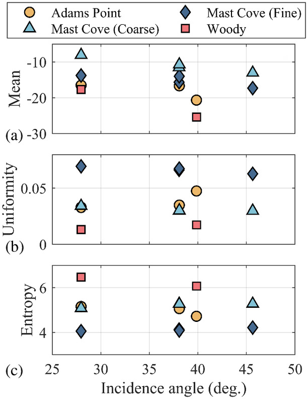
To check whether the incidence angle at which the image was collected influenced the backscatter histograms, the three metrics that exhibited distinct trends for the different sites were plotted against the incidence angle (Fig. 9). With regard to the mean backscatter [Fig. 9(a)], the coarse region of Mast Cove exhibited the highest mean backscatter across all angles, followed by the finer region of Mast Cove, Adams Point, and Woody. Similarly, for the three finer regions (Adams Point, Woody, and the finer region of Mast Cove), the uniformity [Fig. 9(b)] was the highest for the finer region of Mast Cove across all incidence angles, followed by Adams Point, with the lowest values observed at Woody across all incidence angles. Reverse trends were observed for the entropy [Fig. 9(c)], with consistently higher values of entropy for Woody observed across all incidence angles, followed by Adams Point and the finer region of Mast Cove. Finally, in general, consistent trends in the metrics were observed for a given site at a single incidence angle. For example, similar values of entropy (4.09 and 4.13) and uniformity (0.067 and 0.066) were observed for the images from August 6 and 7, 2021, which had the same incidence angle (38.1°) but were from two separate CSK satellites (CSK4 and CSK2, respectively; Table 1). However, slight variations in the mean backscatter were observed (−14 dB and −15.6 dB for the images from August 6 and 7, respectively). This is likely a result of differences in the water levels at the time of imaging (−0.5 m and 0.3 m, respectively; WillyWeather 2023), leading to a different amount of Mast Cove being exposed. Further investigation is required to validate these results.
To distinguish between sites composed of soils of different USCS classifications, the values of entropy and uniformity from each image are plotted against the mean backscatter in Figs. 10(a and b), respectively. These plots clearly show distinct differences between the entropy/uniformity for Adams Point, Woody, and the finer zone of Mast Cove. In both plots, a qualitative boundary between the finer and coarser tidal flats can be drawn at a mean backscatter coefficient of −13.5 dB (solid black line) following the observed trends. While this boundary is lower than the average value observed for beach sands by Dehouck et al. (2011), it is dictated by the mean backscatter from the image from August 8, 2021. The image on this date was collected at a higher incidence angle than the images collected by Dehouck et al. (2011) [45.7° in the present study versus 32°–33° in Dehouck et al. (2011)]. In the three remaining images, the coarse region of Mast Cove exhibited higher backscatter values at Mast Cove than the average values observed by Dehouck et al. (2011); the significant gravel content of the coarser region of Mast Cove likely increased both the surface roughness and the resulting backscatter. For entropy, boundaries can be drawn at 6 to divide Woody and Adams Point and at 4.5 to divide Adams Point and the finer zone of Mast Cove (dashed lines) using the trends observed from Fig. 8(f) to classify the flats according to their USCS classification. A similar process can be repeated for uniformity, with boundaries drawn at 0.055 to separate the finer zone at Mast Cove and Adams Point and at 0.025 to separate Woody and Adams Point, again using the trends observed in Fig. 8(e).

Discussion
The differences in fines content, water content, and USCS classification/index properties between the three sites are likely governed by differences in tidal energy and flow velocity. The lower Piscataqua River portion of the Great Bay [Fig. 1(a)] is a highly dissipative region that behaves like a partially progressive wave, while the Little Bay/Great Bay (inner estuary) section behaves like a standing wave with a lower dissipative regime (Cook et al. 2019; Swift and Brown 1983). Nearly half of the tidal energy at the mouth of the estuary system is lost as the tides travel through the lower Piscataqua River, turn at Dover Point, and move into the inner estuary. In the lower Piscataqua River, the channel depth ranges between 13 m and 26 m and features coarse sediment at the bottom of the deep channels (Cook et al. 2019). The strong maximum tidal currents of up to 2.0 m/s in the lower Piscataqua River prevent most fine sediments from being deposited on flats such as those found at Mast Cove, leading to a higher percentage of coarser sediments.
From sediment sampling, Mast Cove exhibited a high percentage of coarse material (>50%) for both the coarse and fine regions, resulting in all samples being classified as sand (Table 3). The fine region, which occurred closer to the water line at the time of measurements, exhibited moisture contents of 18.1%–48.3%, with fines contents ranging from 14.1% to 44.3%. Conversely, samples from the coarser region exhibited moisture contents of 17.1%–41.4%, with fines contents of 4.1%–43.7%. Five samples from the coarser region of Mast Cove exhibited higher moisture contents (40.0%–41.4%) and fines contents (25.1%–43.7%) than the typical values for this region. These samples were collected near and within the drainage channel (that exhibited active flow during measurements). While it is anticipated that the moisture content would be influenced by proximity to the water line, these results suggest that, for mixed sand flats [sand contents between 30% and 70%, Choi et al. (2011)], proximity to water also strongly influences the fines content.
On the other hand, fine sediments, such as silts and clays, typically settle at very low currents in estuaries (Dronkers 1986). In the main channels of the inner estuary, currents reach a maximum of 0.5 m/s (Ertürk et al. 2002; Swift and Brown 1983) with a maximum channel depth of 10 m (Ertürk et al. 2002). In both the lower Piscataqua River and the inner estuary, the tidal current speeds decrease away from the center of the channel and reach a minimum along the edges of the estuary, leading to the deposition of finer sediments onto the tidal flats such as those found at Adams Point and Woody. While both sites exhibited a high percentage of fines (on average, 89.4% and 98.3% for Adams Point and Woody, respectively) and both classified as fine-grained, silty soils, Atterberg limit testing indicated different USCS classifications with different plasticity characteristics (ML for Adams Point and MH for Woody). This suggests that factors beyond tidal currents may be influencing the type of sediment found at the sites. This may include factors such as benthic biological activity or the presence of vegetation. For example, salt marshes are located near the Woody sample collection sites [Fig. 11(a)], while there are no salt marshes near Adams Point. Thus, the proximity of Woody to salt marshes may impact the sediment type found at the site due to the decomposition of vegetation.

The sediment samples collected represent point measurements and, therefore, small regions of the tidal flats. Conversely, remote sensing can be used to improve the classification of the entire flat. Previous studies primarily focused on identifying the variability of sediments within a single tidal flat (Choe and Kim 2011; Deroin 2012; Gade et al. 2008; Lee et al. 2012; van der Wal et al. 2005; van der Wal and Herman 2007) and did not follow geotechnical sediment classification schemes such as the USCS. These frameworks have applied regression techniques (van der Wal et al. 2005; van der Wal and Herman 2007), backscatter modeling utilizing multipolarized or multifrequency data (Choe and Kim 2011; Deroin 2012; Gade et al. 2008), and decision tree analysis (Lee et al. 2012). However, due to the spatial homogeneity and the relatively small area of the flats investigated in the present study, it is instead of interest to develop a classification scheme where the general soil type of the entire flat can be identified, primarily following the USCS classification and percentages of gravels, sands, and fines using X-band SAR. Of the aforementioned studies, only two applied X-band data: Lee et al. (2012) utilized horizontally co-polarized, vertically co-polarized, and cross-polarized X-band (TerraSAR-X) following a decision tree analysis, while Choe and Kim (2011) only used vertically co-polarized TerraSAR-X data to derive surface parameters. Statistical properties of backscatter for tidal flats environments have only been minimally investigated (Adolph et al. 2018) and have not been widely applied.
Previous work has demonstrated that in intertidal flat environments, the surface roughness and soil texture (i.e., composition) can be derived from SAR images (van der Wal et al. 2005), and along with moisture content, represent the important soil characteristics impacting backscatter (Ulaby et al. 1986). The relationship between water content and fines content presented in Fig. 5 demonstrates that different soil types (sands versus silts) will exhibit different characteristic water contents. While the time of exposure to air of the tidal flat impacts the moisture content and, in turn, affects the backscatter (Lee et al. 2011), the impact in the present study is likely minimal due to the short exposure time for Great Bay sediments (<4 h). Previous studies (Bousbih et al. 2019; Gorrab et al. 2015; Zribi et al. 2012) have demonstrated that soil texture significantly impacts the backscatter, primarily due to the ability of soil to retain water. Fine-grained soils, such as clays, exhibit good water retention capacity and cannot dry as fast as sands (which freely drain). At saturation, clean sands (i.e., limited fines) exhibit moisture contents of approximately 25% (Sherman 1990), while clays can exceed 700%, depending on the mineralogy (Lambe and Whitman 1969); in this study, it was assumed that the sediments were saturated or nearly saturated throughout their entire exposure. Accordingly, sands should exhibit higher backscatter coefficients than muds (Hallikainen et al. 1985), which is consistent with the results presented here. Regression equations from van der Wal et al. (2005) for mud content and backscatter also express this relationship.
The lower mean backscatter values of Adams Point, Woody, and the finer region of Mast Cove are consistent with the higher water contents found at these sites (water contents of 83.2%–119.5%, 105.7%–172.7%, and 18.1%–48.3%, for the three respective sites), especially in comparison with those found in that coarse region of Mast Cove (moisture contents of 17.1%–41.4% and 17.1%–33.6% when excluding the samples collected near and within the drainage channel). Lee et al. (2012) observed slightly higher backscatter values for mud flats (−14.7 dB) than those observed in the present study. This higher backscatter was influenced by site topography and a higher density of tidal channels than that observed in the present study (Choi et al. 2011; Lee et al. 2012). However, Dehouck et al. (2011) observed a mean backscatter of −15.6 dB to −15.5 dB; these values represent the higher end of the backscatter observed (Table 2; Fig. 8). In the present study, the scattering behavior is likely strongly influenced by water ponding within pillow-hollow structures [Fig. 11(b)] where water ponds during ebb tide, representing roughness elements on the order of tens of centimeters horizontally (van der Wal et al. 2005). The impact of ponded water on the backscatter response of muddy tidal flats has been previously observed (Adolph et al. 2018; Kim et al. 2011), with a reduction in the backscatter of 3–7 dB compared to the backscatter response of tidal flats without ponded water (Kim et al. 2011). These bed morphology features have previously been documented at Adams Point (Anderson 1983) and are potentially influenced by rainfall (Anderson 1983) or biological activity (Whitehouse et al. 2000).
In the finer region of Mast Cove, surface water and similar bed morphology features were observed; however, they were less pronounced than those at Adams Point and Woody. The coarser region of Mast Cove did not exhibit noticeable bed morphology features or a significant amount of standing water at the time of measurements and exhibited higher mean backscatter coefficients. The lower percentage of fines likely allows for increased drainage in the coarser region of Mast Cove and limited standing water during low tide. Lee et al. (2012) observed a backscatter of −16.6 dB for mixed flats (sand contents between 30% and 70%; Choi et al. 2011), in line with the mean backscatter values observed for the finer zone of Mast Cove (Table 2). The finer region of Mast Cove would classify as a mixed flat following Choi et al. (2011), indicating that the mean backscatter observed in the present study for the finer zone of Mast Cove is in line with the expected results.
Beyond the mean value of the backscatter, other characteristics of the backscatter histogram, such as uniformity and entropy, as shown in Fig. 8 and Table 2, may be able to provide insight into differentiating between sandy sites with a high fines content (such as the finer region of Mast Cove) and sites that classify as fine-grained (such as Woody and Adams Point). The differences in the trends for these two parameters for the three different finer sites (Figs. 8 and 10) are likely due to variations in the bed morphological features and surface roughness observed at the sites, which is known to impact the backscatter (Ulaby et al. 1986; van der Wal et al. 2005). The high entropy and low uniformity for Woody are likely a result of the sporadic drainage channels found on the site, which result in a more random (higher entropy) and less uniform (low uniformity) backscatter histogram. At Adams Point, where bed features were the most prevalent, intermediate values of uniformity and entropy were observed. These pillow-hollow features occur consistently across the site and appear less random than drainage paths. Both types of surface features typically occur on mudflats and are less common on sandy flats (Dyer 1998; Whitehouse et al. 2000). The low entropy and high uniformity at the finer region of Mast Cove may be due to the limited bed morphology features. Thus, backscatter response histograms with high entropy and low uniformity may aid in identifying muddy environments versus sandy environments with high fines contents. However, it should be noted that whether the differences in entropy and uniformity between Woody (MH with little coarse material) and Adams Point (ML with approximately 10.6% coarse materials) are due to differences in soil classification or bed features is unknown at this time and warrants further investigation.
There are two major shortcomings associated with the use of SAR for the identification of soil types on tidal flats that should be addressed when interpreting results. First, SAR is unable to image through water, meaning that information cannot be collected during flood conditions or times of high water. A second issue with the use of SAR arises from imaging geometry. The landward side of the flats is rimmed by trees that are significantly higher than the mudflats (Fig. 1). Since SAR systems are active sensors, trees will appear to overlay the mudflat, and information related to the soil type cannot be obtained if the incident radar energy images the trees first. This can lead to loss of information in tree-shadow regions of the mudflat for a specific image.
Conclusions
The sediment fines content, moisture content, plasticity, and variability in X-band SAR signals from three distinct intertidal flats in the Great Bay Estuary are investigated. Two sites primarily consist of fine-grained soils (Adams Point, Woody) but with different USCS classifications (ML and MH for Adams Point and Woody, respectively), and one mostly consists of coarse-grained soils of a wide range of grain sizes, fines content, and water contents (Mast Cove; Table 3). Using grain-size analysis, USCS classifications, and the moisture contents, Mast Cove is determined to contain two distinct regions: one comprises a higher percentage of coarse material with lower moisture contents and a range of USCS classifications and one comprises a higher percentage of finer material, higher moisture contents, and a consistent USCS classification of SM. As a complement to in situ sampling, X-band SAR is also explored for characterizing intertidal flats. The percentage of fines impacts the SAR backscatter signals, as previously observed by van der Wal et al. (2005). Tidal flats with higher percentages of fines (Adams Point, Woody) and, therefore, with higher moisture contents generally exhibit lower mean backscatter coefficients compared to a sandier flat with lower moisture contents (coarser region of Mast Cove). The finer region of Mast Cove also generally exhibits lower backscatter coefficients (similar to those found for Adams Point and Woody) compared to the coarser region, which may be a result of the high fines content and moisture content found within this region of Mast Cove. The three finer locations are clearly distinct in terms of the SAR backscatter entropy and uniformity, with Adams Point and Woody exhibiting higher and lower values of entropy and uniformity, respectively, than the finer region of Mast Cove. Geomorphological surface features such as small-scale (tens of centimeters) pillow-hollows or drainage channels, which are common in muddy but not sandy environments, likely impact the histograms of the backscatter coefficient, suggesting that uniformity and entropy can be used to distinguish between sites composed of fine soils (e.g., silts and clays) and coarse sandy soils with a high fines content. These metrics (mean backscatter, uniformity, and entropy) are consistent for a given image incidence angle (Fig. 9) and sensors from the same satellite constellation (Table 1), demonstrating that high-resolution X-band SAR can provide information related to soil classification, fines contents, and general ranges of moisture contents for a given site.
Data Availability Statement
Some or all data, models, or codes generated or used during the study are proprietary or confidential and may only be provided with restrictions. Licensing for satellite images was provided through Grant N00014-18-1-2435 and cannot be shared.
Acknowledgments
The authors thank the Office of Naval Research for funding this work through Grant N00014-18-1-2435. The authors also thank Jon Hunt (UNH) and Liz Smith (VT) for assistance with fieldwork, Majid Ghayoomi (UNH) and Bernardo Castellanos (VT) for assistance with laboratory testing, the Center for Southeastern Tropical Advanced Remote Sensing (CSTARS) for satellite image access, and Albin Rosado (VT) for his contributions to data collection and laboratory testing. Finally, the authors thank the two anonymous reviewers and the associate editor for their input that helped improve the quality of this manuscript.
References
Adolph, W., H. Farke, S. Lehner, and M. Ehlers. 2018. “Remote sensing intertidal flats with TerraSAR-X. A SAR perspective of the structural elements of a tidal basin for monitoring the wadden sea.” Remote Sens. 10 (7): 1085. https://doi.org/10.3390/rs10071085.
Anderson, F. E. 1983. “The northern muddy intertidal: Seasonal factors controlling erosion and deposition—A review.” Can. J. Fish. Aquat. Sci. 40 (S1): s143–s159. https://doi.org/10.1139/f83-277.
ASTM. 2005. Standard test methods for liquid limit, plastic limit, and plasticity index of soils. ASTM D4318-17e1. West Conshohocken, PA: ASTM.
ASTM. 2017a. Standard test methods for particle-size distribution (gradation) of soils using sieve analysis. ASTM D6913. (Reapproved 2009): 1–35. West Conshohocken, PA: ASTM.
ASTM. 2017b. Standard practice for classification of soils for engineering purposes (unified soil classification system). ASTM D2487-17. West Conshohocken, PA: ASTM.
ASTM. 2017c. Standard test methods for amount of material in soils finer than the No. 200 (75-µm). ASTM D1140-17. West Conshohocken, PA: ASTM.
Baghdadi, N., M. Zribi, C. Loumagne, P. Ansart, and T. P. Anguela. 2008. “Analysis of TerraSAR-X data and their sensitivity to soil surface parameters over bare agricultural fields.” Remote Sens. Environ. 112 (12): 4370–4379. https://doi.org/10.1016/j.rse.2008.08.004.
Bilgili, A., J. A. Proehl, D. R. Lynch, K. W. Smith, and M. R. Swift. 2005. “Estuary/ocean exchange and tidal mixing in a Gulf of Maine Estuary: A Lagrangian modeling study.” Estuarine Coastal Shelf Sci. 65 (4): 607–624. https://doi.org/10.1016/j.ecss.2005.06.027.
Bilgili, A., M. R. Swift, D. R. Lynch, and J. T. C. Ip. 2003. “Modeling bed-load transport of coarse sediments in the Great Bay Estuary, New Hampshire.” Estuarine Coastal Shelf Sci. 58 (4): 937–950. https://doi.org/10.1016/j.ecss.2003.07.007.
Boumboulis, V., D. Apostolopoulos, N. Depountis, and K. Nikolakopoulos. 2021. “The importance of geotechnical evaluation and shoreline evolution in coastal vulnerability index calculations.” J. Mar. Sci. Eng. 9 (4): 423. https://doi.org/10.3390/jmse9040423.
Bousbih, S., M. Zribi, C. Pelletier, A. Gorrab, Z. Lili-Chabaane, N. Baghdadi, N. Ben Aissa, and B. Mougenot. 2019. “Soil texture estimation using radar and optical data from Sentinel-1 and Sentinel-2.” Remote Sens. 11 (13): 1520. https://doi.org/10.3390/rs11131520.
Choe, B.-H., and D.-J. Kim. 2011. “Retrieval of surface parameters in tidal flats using radar backscattering model and multi-frequency SAR data.” Korean J. Remote Sens. 27: 225–234. https://doi.org/10.7780/kjrs.2011.27.3.225.
Choi, J.-K., J. Eom, and J.-H. Ryu. 2011. “Spatial relationships between surface sedimentary facies distribution and topography using remotely sensed data: Example from the Ganghwa tidal flat, Korea.” Mar. Geol. 280 (1–4): 205–211. https://doi.org/10.1016/j.margeo.2010.10.022.
Cook, S. E., T. C. Lippmann, and J. D. Irish. 2019. “Modeling nonlinear tidal evolution in an energetic estuary.” Ocean Modell. 136: 13–27. https://doi.org/10.1016/j.ocemod.2019.02.009.
Dehouck, A., V. Lafon, N. Baghdadi, A. Roubache, and T. Rabaute. 2011. “Potential of TerraSAR-X imagery for mapping intertidal coastal wetlands.” In Proc., 4th TerraSAR-X Science Team Meeting. Oberpfaffenhofen, Germany: German Aerospace Center.
Deroin, J.-P. 2012. “Combining ALOS and ERS-2 SAR data for the characterization of tidal flats. Case study from the Baie des Veys, Normandy, France.” Int. J. Appl. Earth Obs. Geoinf. 18: 183–194. https://doi.org/10.1016/j.jag.2012.01.019.
Domenech, M. B., N. M. Amiotti, J. L. Costa, and M. Castro-Franco. 2020. “Prediction of topsoil properties at field-scale by using C-band SAR data.” Int. J. Appl. Earth Obs. Geoinf. 93: 102197. https://doi.org/10.1016/j.jag.2020.102197.
Dronkers, J. 1986. “Tidal asymmetry and estuarine morphology.” Netherlands J. Sea Res. 20 (2–3): 117–131. https://doi.org/10.1016/0077-7579(86)90036-0.
Dunn, I. S. 1959. “Tractive resistance of cohesive channels.” J. Soil Mech. Found. Div. 85 (3): 1–24. https://doi.org/10.1061/JSFEAQ.0000195.
Dyer, K. R. 1998. “The typology of intertidal mudflats.” Geol. Soc. London Spec. Publ. 139: 11–24. https://doi.org/10.1144/GSL.SP.1998.139.01.02.
Ertürk, Ş. N., A. Bilgili, M. R. Swift, W. S. Brown, B. Çelikkol, J. T. C. Ip, and D. R. Lynch. 2002. “Simulation of the Great Bay Estuarine System: Tides with tidal flats wetting and drying.” J. Geophy. Res. 107 (C5): 3038. https://doi.org/10.1029/2001JC000883.
Fagherazzi, S., T. Viggato, A. M. Vieillard, G. Mariotti, and R. W. Fulweiler. 2017. “The effect of evaporation on the erodibility of mudflats in a mesotidal estuary.” Estuarine Coastal Shelf Sci. 194: 118–127. https://doi.org/10.1016/j.ecss.2017.06.011.
Gade, M., W. Alpers, C. Melsheimer, and G. Tanck. 2008. “Classification of sediments on exposed tidal flats in the German Bight using multi-frequency radar data.” Remote Sens. Environ. 112 (4): 1603–1613. https://doi.org/10.1016/j.rse.2007.08.015.
Gorrab, A., M. Zribi, N. Baghdadi, B. Mougenot, P. Fanise, and Z. Chabaane. 2015. “Retrieval of both soil moisture and texture using TerraSAR-X images.” Remote Sens. 7 (8): 10098–10116. https://doi.org/10.3390/rs70810098.
Hallikainen, M., F. Ulabz, M. Dobson, M. El-Rayes, and L.-k. Wu. 1985. “Microwave dielectric behavior of wet soil—Part 1: Empirical models and experimental observations.” IEEE Trans. Geosci. Remote Sens. GE-23 (1): 25–34. https://doi.org/10.1109/TGRS.1985.289497.
Han, D., F. Vahedifard, and J. V. Aanstoos. 2017. “Investigating the correlation between radar backscatter and in situ soil property measurements.” Int. J. Appl. Earth Obs. Geoinf. 57: 136–144. https://doi.org/10.1016/j.jag.2016.12.018.
Kim, D.-j., W. M. Moon, G. Kim, S.-E. Park, and H. Lee. 2011. “Submarine groundwater discharge in tidal flats revealed by space-borne synthetic aperture radar.” Remote Sens. Environ. 115 (2): 793–800. https://doi.org/10.1016/j.rse.2010.11.009.
Lambe, T. W., and R. V. Whitman. 1969. Soil mechanics. Hoboken, NJ: Wiley.
Lee, H., H. Chae, and S.-J. Cho. 2011. “Radar backscattering of intertidal mudflats observed by radarsat-1 SAR images and ground-based scatterometer experiments.” IEEE Trans. Geosci. Remote Sens. 49 (5): 1701–1711. https://doi.org/10.1109/TGRS.2010.2084094.
Lee, Y.-K., J.-W. Park, J.-K. Choi, Y. Oh, and J.-S. Won. 2012. “Potential uses of TerraSAR-X for mapping herbaceous halophytes over salt marsh and tidal flats.” Estuarine Coastal Shelf Sci. 115: 366–376. https://doi.org/10.1016/j.ecss.2012.10.003.
Marzahn, P., and S. Meyer. 2020. “Utilization of multi-temporal microwave remote sensing data within a geostatistical regionalization approach for the derivation of soil texture.” Remote Sens. 12 (16): 2660. https://doi.org/10.3390/RS12162660.
Sabins, F. F. 2007. Remote sensing: Principles and interpretation. Long Grove, IL: Waveland Press.
Sherman, D. J. 1990. “Evaluation of aeolian sand transport equations using intertidal-zone measurements, Saunton Sands, England.” Sedimentology 37 (2): 385–392. https://doi.org/10.1111/j.1365-3091.1990.tb00967.x.
Swift, M. R., and W. S. Brown. 1983. “Distribution of bottom stress and tidal energy dissipation in a well-mixed estuary.” Estuarine Coastal Shelf Sci. 17 (3): 297–317. https://doi.org/10.1016/0272-7714(83)90024-0.
Ulaby, F. T., R. K. Moore, and A. K. Fung. 1986. Microwave remote sensing: Active and passive, volume 3 volume scattering and emission theory, advanced systems and applications. Reading, MA: Addison-Wesley.
van der Wal, D., and P. M. J. Herman. 2007. “Regression-based synergy of optical, shortwave infrared and microwave remote sensing for monitoring the grain-size of intertidal sediments.” Remote Sens. Environ. 111 (1): 89–106. https://doi.org/10.1016/j.rse.2007.03.019.
van der Wal, D., P. M. J. Herman, and A. Wielemaker-van den Dool. 2005. “Characterisation of surface roughness and sediment texture of intertidal flats using ERS SAR imagery.” Remote Sens. Environ. 98 (1): 96–109. https://doi.org/10.1016/j.rse.2005.06.004.
Veci, L. 2019. SENTINEL-1 toolbox SAR basics tutorial. Paris, France: ARRAY Systems Computing, Inc. and European Space Agency.
Wengrove, M. E., D. L. Foster, L. H. Kalnejais, V. Percuoco, and T. C. Lippmann. 2015. “Field and laboratory observations of bed stress and associated nutrient release in a tidal estuary.” Estuarine Coastal Shelf Sci. 161: 11–24. https://doi.org/10.1016/j.ecss.2015.04.005.
Whitehouse, R. J. S., P. Bassoullet, K. R. Dyer, H. J. Mitchener, and W. Roberts. 2000. “The influence of bedforms on flow and sediment transport over intertidal mudflats.” Cont. Shelf Res. 20 (10–11): 1099–1124. https://doi.org/10.1016/S0278-4343(00)00014-5.
WillyWeather. 2023. “Piscataqua river-mast cove.” WillyWeather. Accessed November 10, 2023. https://tides.willyweather.com/me/york-county/piscataqua-river-mast-cove.html.
Winterwerp, J. C., W. G. M. van Kesteren, B. van Prooijen, and W. Jacobs. 2012. “A conceptual framework for shear flow–induced erosion of soft cohesive sediment beds.” J. Geophys. Res.: Oceans 117: 1–17. https://doi.org/10.1029/2012JC008072.
Zribi, M., F. Kotti, Z. Lili-Chabaane, N. Baghdadi, N. Ben Issa, R. Amri, B. Amri, and A. Chehbouni. 2012. “Soil texture estimation over a semiarid area using TerraSAR-X radar data.” IEEE Geosci. Remote Sens. Lett. 9 (3): 353–357. https://doi.org/10.1109/LGRS.2011.2168379.
Information & Authors
Information
Published In

Journal of Waterway, Port, Coastal, and Ocean Engineering
Volume 150 • Issue 4 • July 2024
Copyright
This work is made available under the terms of the Creative Commons Attribution 4.0 International license, https://creativecommons.org/licenses/by/4.0/.
History
Received: Aug 4, 2023
Accepted: Mar 11, 2024
Published online: Apr 4, 2024
Published in print: Jul 1, 2024
Discussion open until: Sep 4, 2024
ASCE Technical Topics:
- Coastal engineering
- Coasts, oceans, ports, and waterways engineering
- Engineering fundamentals
- Estuaries
- Field tests
- Geomechanics
- Geotechnical engineering
- Hydrologic engineering
- Hydrologic properties
- Hydrology
- River engineering
- Sediment
- Silt
- Soil classification
- Soil mechanics
- Soil properties
- Soil water
- Soils (by type)
- Tests (by type)
- Water and water resources
- Water content
Authors
Metrics & Citations
Metrics
Citations
Download citation
If you have the appropriate software installed, you can download article citation data to the citation manager of your choice. Simply select your manager software from the list below and click Download.