Combining Socioeconomic, Demographic, and Zoning Data to Explore Urban Inequality in Pittsburgh
Publication: Journal of Urban Planning and Development
Volume 150, Issue 1
Abstract
Historic injustices due to racial discrimination, redlining, and inequitable zoning practices have contributed to urban inequalities in the United States. These inequalities have been compounded by a lack of consideration for how infrastructure, industrial projects, and zoning impact nearby low-income and minority populations. To promote an equitable future, this paper investigates whether there are spatial patterns based on zoning variance data in the city of Pittsburgh. The authors used principal component analysis and regression analysis to study statistical correlations between socioeconomic and demographic characteristics and zoning variance application data. Several relationships reflect statistical significance, such as the average income of the residents and the percentage over the age of 25 who are college-educated, while the overall results highlight potential future research areas. Our work combining data sets with spatially explicit statistical analysis has the potential to equip decision makers with future tools necessary to account for inequalities and assess communities that may be unaware of the opportunities that variances present.
Introduction
Redlining and zoning practices have historically divided urban areas by race and class, resulting in significant neighborhood disparities that exist today. Numerous studies have explored these inequalities through the specified lens of redlining and exclusionary zoning (Moga 2017; Pendall 2000; Shertzer et al. 2021; Whittemore 2017b; Woods 2012; Young 2005). These historical practices have resulted in a wide array of adverse health, economic, and quality of life implications for marginalized residents (Farber 1998; Hughey et al. 2016; Martenies et al. 2017; Moreno et al. 2004; Patterson and Harley 2019; Rothwell and Massey 2009; Sabrin et al. 2020; Sallis et al. 2012; Voelkel et al. 2018). To address these inequalities, it is critical to find ways to understand, quantify, and map them to provide tools for community action.
While historical records clearly show patterns of exclusionary zoning and redlining practices that marginalized certain communities (Shertzer et al. 2016; Whittemore 2017b), further research is necessary to understand the subtleties of current behavior and practices. Previous work that examined the potential to map urban diversity and various socioeconomic variables across census tract groups sought to equip planners with information that could promote diversity (Talen 2005). This approach promoted providing urban planners with data that could help enable more equitable practices, including support for zoning reforms (Talen 2005). Researchers have also considered how zoning practices have allowed the siting of noxious facilities to inequitably burden already marginalized communities (Lejano and Iseki 2001; Whittemore 2017a). These facilities can pose health risks and lower the quality of life for these communities, creating inequitable environmental and health burdens. In addition to understanding historical behaviors, understanding how these practices might occur in the present or evolve in the future can contribute new knowledge in this landscape. Furthermore, zoning practices can differ widely between regions and even within the same city, making it imperative to have localized studies that reflect these nuances.
A less examined area in the literature is the impact of zoning variances and how these exceptions to a zoning code may be advantageous or disadvantageous to specific population groups. A variance is a form of zoning relief, a permitted violation of the zoning code that residents or local actors may apply for through a quasi-judicial Zoning Board of Adjustments (ZBA) or similarly named body to circumvent zoning ordinances (Shapiro 1969). Variance decisions are historically made with little juridical oversight and generally high approval rates (Fischer et al. 2018). As locals, communities, or developers must seek out these variances, they introduce an area of development that is largely motivated or stagnant, depending on these individuals. Variance applications of local members or communities may improve residential homes or local businesses, while others, potentially made by outside developers, commercial actors, or absentee owners, may inadvertently hinder the local population. Fischer et al. (2018) examined zoning variances in New York City over nearly 20 years, concluding that the zoning relief process produces unequal outcomes playing upon already present inequalities, and they urged further focus from planners concerning this zoning method.
Social vulnerability measures combined with zoning variance data have the potential to unlock new insights into present-day zoning practices. An urban region's social vulnerability can be quantified through tools such as index-based measures of various socioeconomic and demographic indicators. Cutter et al. (2003) created a social vulnerability index (SVI) with a wide array of indicators based on various fields of application (Comfort et al. 1999). These indices are often mapped to specific block or tract groups to show spatially how vulnerability levels are dispersed across a larger region of interest (Brunetta and Salata 2019; Garbutt et al. 2015; Nelson et al. 2015). By using mapping tools, complex data can be related to space in a succinct and comprehensible way, providing planners the opportunity to integrate the data into their development processes (Carmona 2014).
Building upon these literature gaps, this case study examines the integration of zoning variance data from the city of Pittsburgh with social vulnerability using mapping tools and regression analysis. We propose a new social vulnerability index that leverages existing methods and expands them to include specific socioeconomic indicators revolving around housing and development data. This paper illustrates the connection between zoning variance data and social vulnerability in such a way that has the potential to inform urban planners. This methodology, promoting equity in urban development, could be applicable in various urban settings.
Methods
Site Description
This research focuses on the city of Pittsburgh. Pittsburgh is located in Allegheny County, just west of the Allegheny Mountain range (Fig. 1). The population of the city of Pittsburgh itself is about 303,000 people over a land area of 143.5 square kilometers. When originally appraised by the Home Owners' Loan Corporation (HOLC) in the 1930s, a segregated housing market divided the city extensively, with 70% of the black residents living in just three of the city's neighborhoods (Rutan and Glass 2018). The redlined maps resulting from this appraisal only prolonged the economic divisions, which depended so much upon regional demographics (Fig. 2). Rutan and Glass (2018) specifically show that in Pittsburgh, the initially deemed hazardous regions from the HOLC map still correlate today to persistently black populations, while the initially deemed best regions continue to correlate to the wealthiest tracts. These findings display how these past investment assessments based upon racial biases have led to lingering inequalities in Pittsburgh. Similarly, researchers have shown that these historic appraisals from the HOLC and zoning decisions that exacerbated racial segregation have resulted in continued disadvantaged regions throughout many US cities, including Pittsburgh, today (Whittemore 2017b; Young 2005).
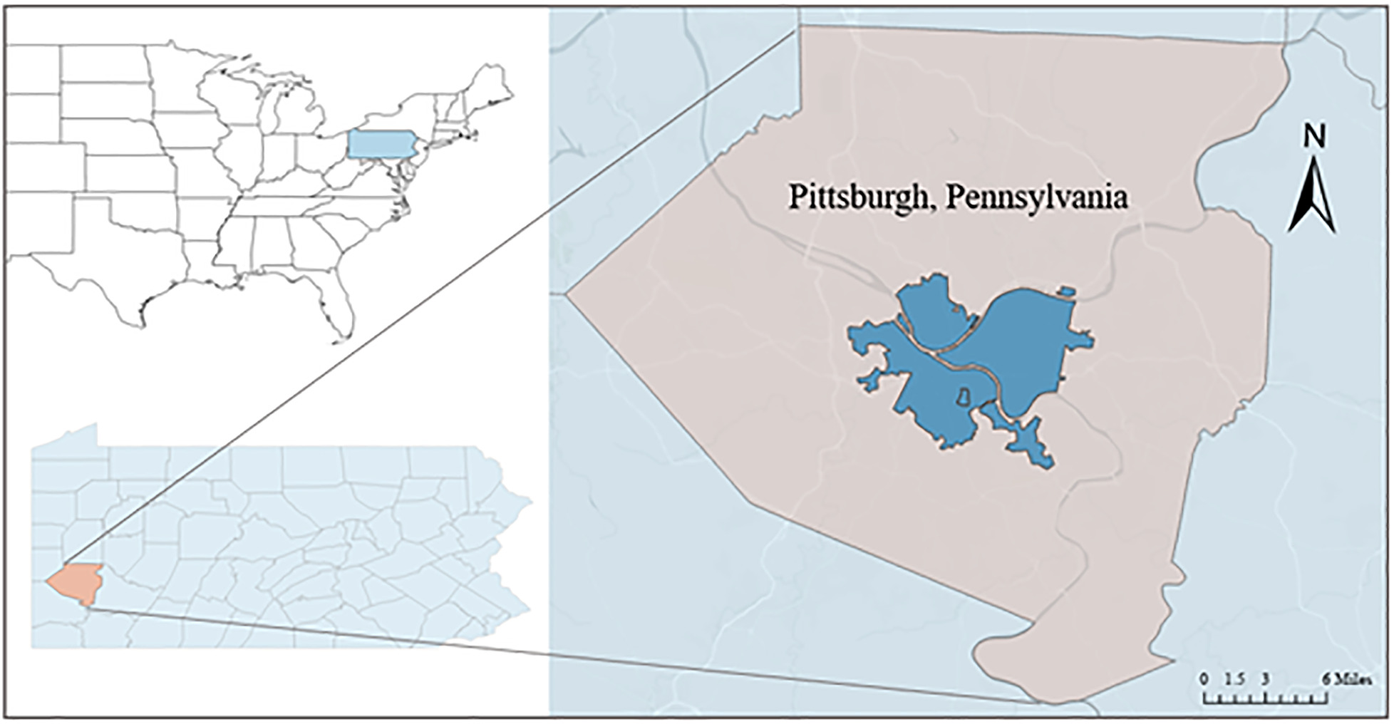
Fig. 1. Pittsburgh, located in Allegheny County in the United States.
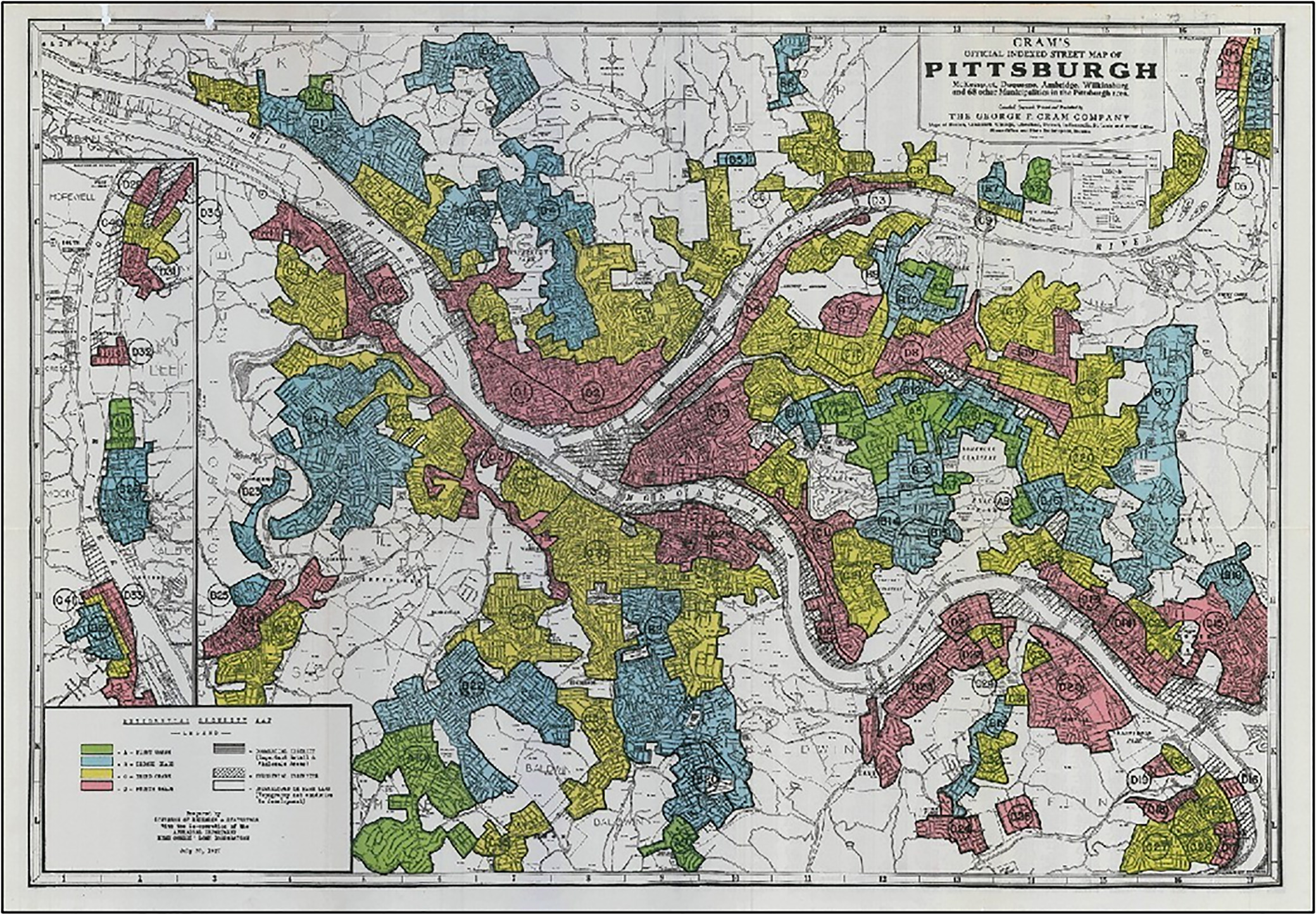
Fig. 2. Residential Security Map of Pittsburgh.
[Reprinted from Nelson et al. (2022), under Creative Commons-BY-4.0 license (https://creativecommons.org/licenses/by/4.0/).]
Pittsburgh is an apt location for this study as historical inequalities are known to exist, and the industrial foundation of the city makes the region especially intriguing to modern urban planners and engineers (Rutan and Glass 2018). Further, the ZBA of Pittsburgh, an adjudicative body within the department of city planning that reviews and decides upon zoning variance applications, is active and transparent. This case study combines multidimensional socioeconomic and demographic census data with Pittsburgh's available zoning exemption data to discover potential relationships.
Zoning Variance Data
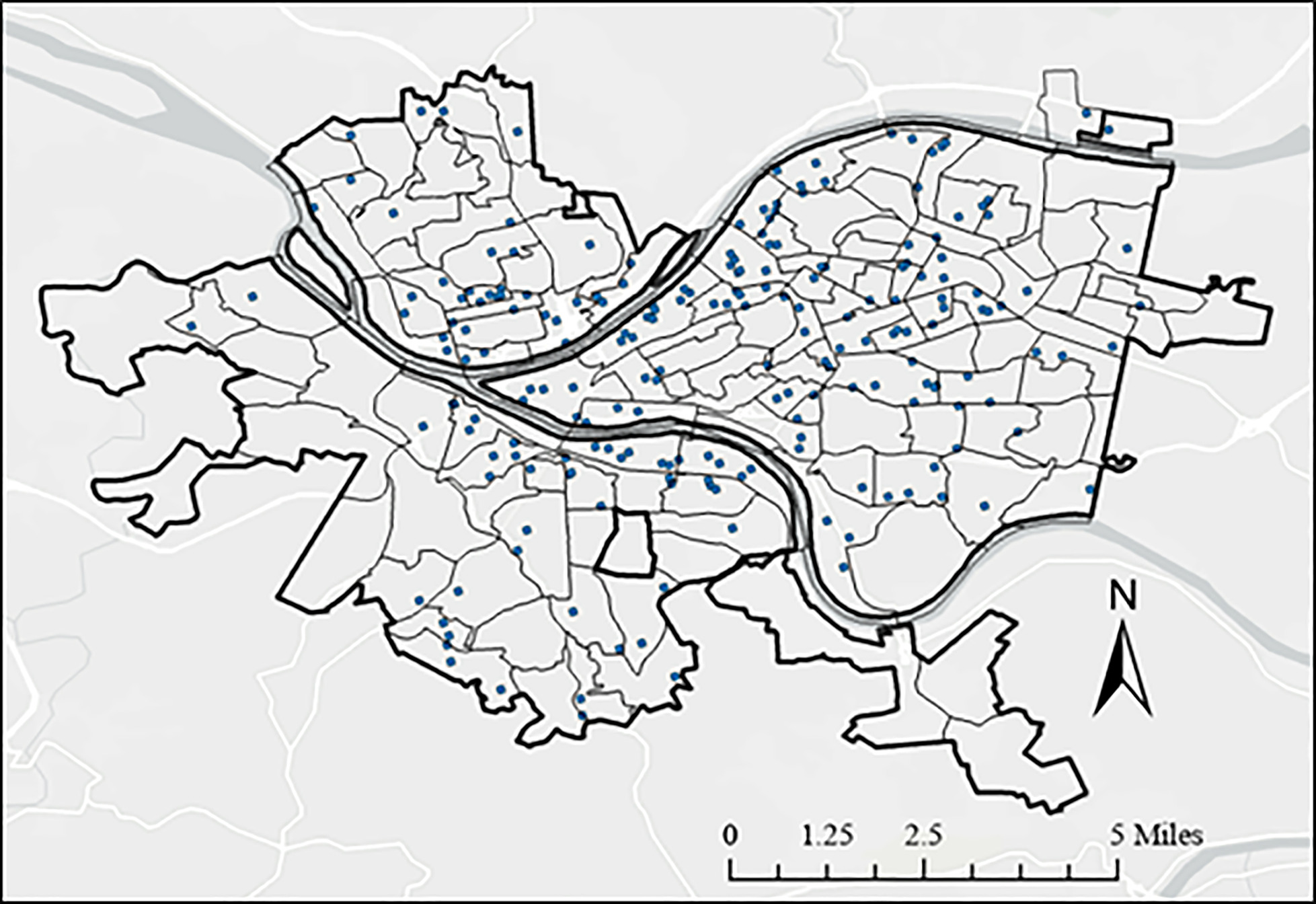
This study utilized variance data for the City of Pittsburgh, which contains information on 210 ZBA applications from 2020 (Supplemental Material Section 2.1 ). Details within the application include the address of the appeal, the applicable zoning code section, the type of appeal, and the result of the case. Appeal types range from a new single-family dwelling to parking space changes or new buildings to new generators or signs. All appeals request an exemption from the zoning code, given the desired changes do not meet the current zoning code and, as such, require special permission from the ZBA before further action. The variance application data were geocoded in ArcGIS Pro Version 2.8.0 (Fig. 3).
Zoning Social Vulnerability Index
To consider the regional demographics surrounding these zoning variances, we utilized an SVI to quantify vulnerability. SVIs are widely utilized metrics that policymakers, designers, and other decision makers can use to propose tailored solutions for higher-risk communities (Brunetta and Salata 2019; Comfort et al. 1999; Cutter et al. 2013; Garbutt et al. 2015; Nelson et al. 2015; Sabrin et al. 2020). Based on similar vulnerability studies, we selected 12 variables at the census tract level from the 2019 US Census Bureau American Community Survey (ACS) to quantify vulnerability. The SVI was created using principal component analysis (PCA), which reduces the dimensionality of the data following the SoVI methodological approach developed by Cutter et al. (2003) and USC (2022). We employed a PCA with a varimax rotation and Kaiser criterion for component selection (Supplemental Material Section 3.1 ).
The PCA resulted in four principal components (PCs) accounting for 74.13% of the variability in the data. Each PC was defined based on its makeup of factors and assigned influence of cardinality on the SVI. A zoning-specific SVI (zSVI) was computed by combining the scores based on their directional adjustments in an additive model. Once calculated, the zSVI results by census tracts were spatially mapped in ArcGIS Pro Version 2.8.0.
Regression Analysis
To study the relationship between the number of variance applications and the tract-level social vulnerability, we performed a series of simple and multiple linear regressions. Regression analyses were performed in Python Version 3.8.6 using the statsmodels package (Seabold and Perktold 2010). The coefficient of determination (R2) value and p-values determined the quality of the model's overall fit and the significance of the relationship between predictor and response variables, respectively.
We used simple linear regressions to examine the relationships between zoning variances and census data. The first regression considered the zSVI as the dependent variable and the number of applied-for zoning variances as the independent variable. This relationship was examined continuously and categorically: first without binning the levels of vulnerability and by simply taking the number of applied-for variances per tract, and then by binning the levels of vulnerability and considering the number of applied-for variances per bin. The study applied three different binning methods: binning by standard deviation, geometric intervals, and quantile distribution, all prioritizing a consistent frequency of variance data points per bin, to compare results between the different ways of grouping the data set.
Further, we conducted multiple linear regressions to examine the relationship between the number of variances per tract and, first, the individual PCs and then, second, the census variables originally considered in the PCA. By doing so, the study examined progressively more detailed relationships. The zSVI simplified the multidimensional sociodemographic data into one vulnerability indicator. The individual PCs reflected 4 different dimensions of vulnerability, and the original 12 census variables displayed the fullness of the data directly. By conducting regression analyses with each of these levels of greater dimensions, the authors hoped to learn more about possible relationships in the data. In this case, the dependent variable is that of the number of zoning variances per tract, and it is tested with the individual PCs and then also the original suite of independent socioeconomic and demographic census variables.
Results
The PCA resulted in a zSVI that characterized Pittsburgh's social vulnerability in relation to zoning. The regression analyses provided statistical insight into the potential relationships between the zoning variances and the census data that comprised the zSVI. Although the zSVI did capture the majority of the variability of the census data, the study found that it was necessary to examine the census data more granularly to determine statistically significant relationships with the zoning variance applications. Several individual census variables displayed a statistically significant relationship with the variance applications in Pittsburgh.
Principal Component Analysis Results
Our PCA resulted in four principal components that all correspond to an increase in vulnerability and, when summed, result in an overall index that increases with higher levels of vulnerability: the higher the index value, the higher the region's zoning vulnerability (Table 1).
| PC # | Name | % variance explained | Factors (weight) | Cardinality |
|---|---|---|---|---|
| 1 | Race, education, and income | 29.45 | % Black (0.82) % Educated (−0.82) Poverty rate (0.71) Vacancy rate (0.70) Average income (−0.57) | + |
| 2 | Housing | 20.51 | % multifamily housing units (0.92) Rental rate (0.91) Black homeownership rate (−0.62) | + |
| 3 | Old units | 12.41 | % Old units (0.92) | + |
| 4 | Ethnic minorities | 11.75 | % Hispanic/Latino (0.84) % American Indian or Alaskan Native (0.80) | + |
Figs. 4(a–d) show each of the individual PCs mapped out. These different maps reflect how each component displays a different aspect of the final index. Figs. 4(a and b) show an increase in vulnerability concentrated at the center of the city, depicting the PCs that deal with race, education, income, and housing. These PCs also display tracts with the highest standard deviation values northeast of the river intersection [Figs. 4(a and b)], while Figs. 4(c and d) show more dispersed vulnerabilities depicting old housing units and ethnic minorities, specifically Hispanic/Latino and American Indian/Alaskan native populations. These results seem to show less vulnerable populations with regard to old units on the outskirts of the city limits with fairly average vulnerability levels across most of the city [Fig. 4(c)]. Additionally, it seems there are low levels of vulnerability dependent upon the ethnic minorities of PC 4, with hotspots in four specific tracts [Fig. 4(d)]. Fig. 4(e) shows the finalized zSVI and the location of the applied-for zoning variances. The gray tracts are those that did not have demographic data available due to a lack of residential areas.
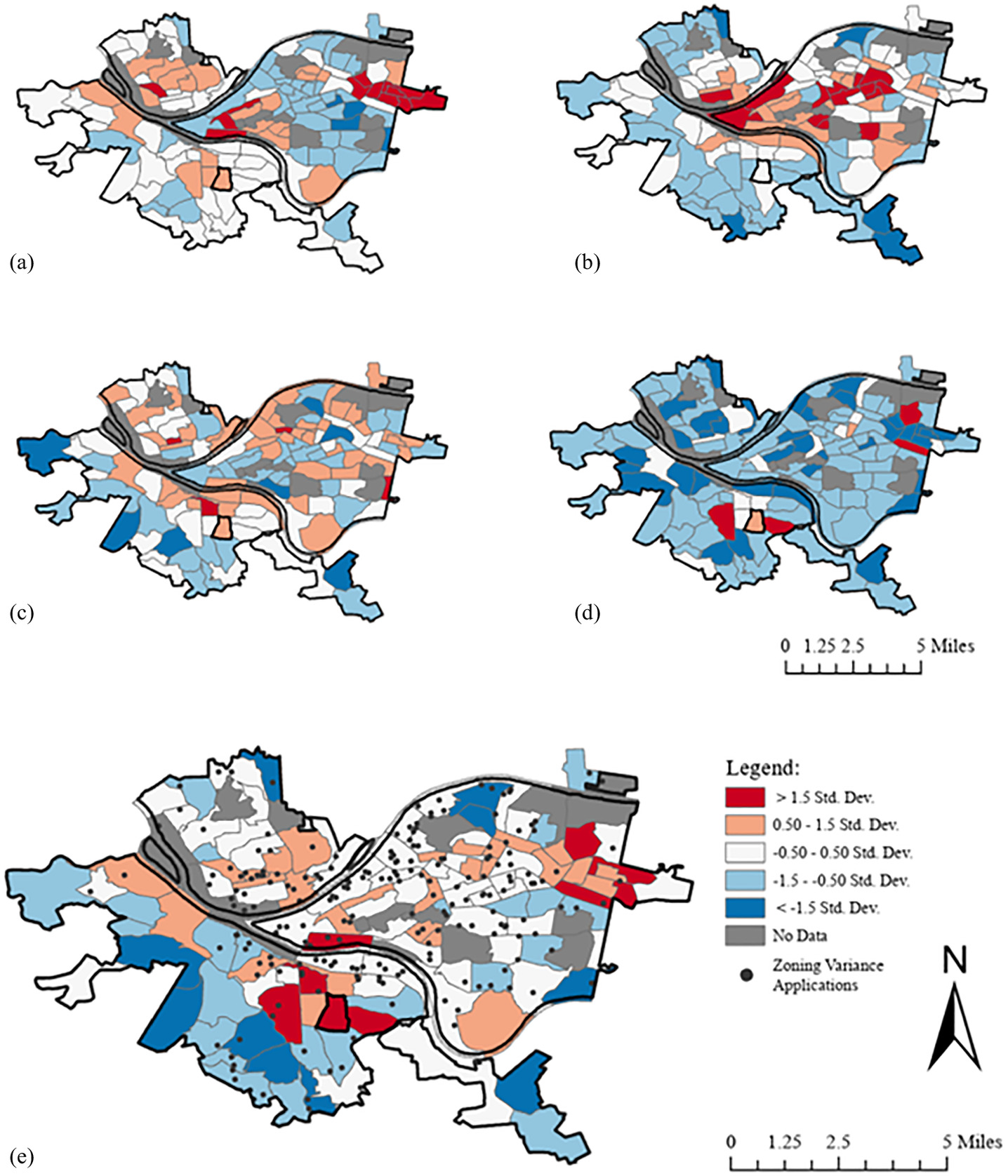
We can compare these five maps shown in Figs. 2–4, the Residential Security Map of Pittsburgh. It is notable that Components 1 and 2 both show similarities to the HOLC map, and it seems reasonable that Component 2 appears to be most similar as it is the Housing component. The overall zSVI map is comparable to the original Residential Security Map as the originally poorer graded regions reflect index scores that are persistently higher than the mean. By understanding regional vulnerability, engineers, designers, and decision makers can more aptly implement solutions to address community needs.
While it is helpful to visualize the location of applied-for variances in the context of the zSVI, these maps alone do not indicate whether a relationship exists between the two. As such, the regression analyses supply statistical insight.
Regression Analysis Results
Simple Linear Regression
To study the relationship between social vulnerability and zoning variance applications in Pittsburgh, we utilized a simple linear regression model where the zSVI is the dependent variable, and the number of applied-for variances per tract is the independent variable. Our analysis found no significant relationship between the zoning vulnerability index and the number of applied-for variances per tract (see details in Supplemental Material Section 3.4 ). Interestingly, the number of applied-for variances is concentrated about a zSVI of 0 with a lower number of applied-for variances in the low and high ends of the zSVI. However, it is noted that tracts with higher vulnerability levels show a slightly greater number of zoning variance applications.
Binned Simple Linear Regressions
With the distribution and lack of relationship observed from the continuous simple regression, we then binned the zSVI to see a distinct distribution of the data and conduct further regressions. The regressions displayed that none of the three binning methods resulted in statistically significant relationships at the 95% confidence level between the zSVI and the number of variance applications per tract; thus, we cannot conclude that there is a statistically significant relationship between the zSVI and the number of applied variances per tract.
After conducting these simple linear regressions and finding a lack of statistically significant relationships, it was deemed necessary to consider the components of the zSVI to observe if any statistical relationships exist at a more granular level. Multiple linear regressions served to examine more complex models of fit.
Multiple Linear Regressions with Individual Principal Components
Examining the number of zoning variance applications against the four individual PCs expands the analysis to a multiple linear regression with the statistical summary in Table 2. As this study is not looking to predict future behavior, our focus is not on the magnitude of the R2 term but on the coefficients and p-values of the independent variables. As such, the analysis reflects a statistically significant relationship between the number of variance applications per tract and that tract's second and third PCs.
| Variables | Coefficients |
|---|---|
| Principal component 1 | −0.4574 |
| Principal component 2 | 0.6730** |
| Principal component 3 | 0.5784* |
| Principal component 4 | −0.1227 |
| R2 | 0.131 |
| Adjusted R2 | 0.101 |
| F-statistic | 4.440 |
Note: *p < 0.05; and **p < 0.01.
PC 2 is termed the housing component as it includes the factors of multifamily housing units, rental rate, and black homeownership rate. A positive cardinality associated with this PC indicates that an increase in value corresponds to an increase in social vulnerability, as found in the PCA. Here, the positive regression coefficient and statistically significant relationship of the variable based on the p-value communicate that with an increase in this PC, an increase in the number of zoning variance applications in the region is expected. This finding agrees with our initial hypothesis that vulnerable neighborhoods, lower income, higher rental rates, and higher minority ownership would correspond to more variance applications, as in these areas, more outside actors have the means to make zoning changes. Owners of rental units and commercial actors have the financial means and political know-how to apply for variances to potentially introduce changes that may not meet the strict zoning code standards.
PC 3 corresponds to the percentage of old units, which is the percentage of housing units built before 1940. Like PC 2, this component has a positive cardinality and relates to a statistically significant positive regression coefficient. Considering that older housing units may have been built initially under different zoning requirements and may more frequently require updates and modifications, it is unsurprising that there is a positive relationship here with the number of applied-for zoning variances.
PC 1 has a p-value of 0.053, making it very nearly significant based on our decided probability value of 95%. This weak significance implies that the factors included in PC 1, having to do with race, education, and income, may have relationships with the number of zoning variances in a region. In contrast, PC 4 has a very high p-value, signifying no significant relationship to the number of zoning variance applications per tract.
Multiple Linear Regressions with Sociodemographic Variables
While the previous multiple linear regression was insightful into the impact of the individual PCs, the data could still be analyzed at a more granular level to examine the individual socioeconomic and demographic indicators. The original 12 variables were the independent variables of the final regression of this study. Table 3 shows the statistical summary of this regression, revealing statistically significant relationships between the indicator variables and the number of applied-for variances in Pittsburgh. The R2 term was the highest yet because each of the variables allowed a degree of freedom for the coefficients to tweak the equation of fit.
| Variables | Model |
|---|---|
| Percent Black | −0.0218* |
| Percent Hispanic/Latino | −0.2512* |
| Percent American Indian/Alaskan Native | −0.0599 |
| Percent immigrant | −0.0663 |
| Average income (density function) | −12.156** |
| Poverty rate | −0.0329* |
| Black homeownership rate | −0.0006 |
| Percent old units | 0.0225* |
| Rental rate | 0.0429* |
| Vacancy rate | 0.0391 |
| Percent multifamily housing units | 0.0008 |
| Percent over 25 educated | 0.0362** |
| R2 | 0.646 |
| Adjusted R2 | 0.607 |
| F-statistic | 16.71 |
Note: *p < 0.05; and **p < 0.01. Income is not a percentage like other variables but a density function, making its magnitude smaller and coefficient value significantly higher.
First, considering the variables that show themselves to be statistically significant, both percent Black and percent Hispanic/Latino are negatively correlated (p < 0.05) with the number of variance applications. This inverse relationship suggests that the regions with higher percentages of minorities have fewer zoning variance applications. Similarly, the region's average income and poverty rate are also significantly and negatively related to the number of variance applications. This relationship seems to suggest that the number of variance applications is lower in poorer communities, which corresponds to historically observed trends that less affluent populations, such as minority populations, are potentially unable to advocate for themselves to the same extent that other neighborhoods may be able to, resulting in fewer variance applications. Although such reasoning may explain this inverse relationship, this result seemingly contradicts the positive relationship between the number of variance applications and the second PC.
Another sociodemographic indicator, the rental rate, is significantly and positively correlated with the number of variance applications. Generally, a higher rental rate corresponds to a lower average income and a higher percentage of minority residents. Hence, the authors expected these indicators to behave similarly to the number of variance applications, but this is not the case. Further, the positive relationship with higher rental rates indicates that larger actors, apartment building owners, and commercial owners proximate to less well-off neighborhoods with higher rental rates would have the political know-how and financial means to apply for more variances.
The percentage of old units and individuals over 25 years old with a bachelor's degree or higher are positively and significantly related to the number of zoning variance applications. This relationship corresponds to what the authors would expect as the previous multiple regression analysis identified PC 3 (percent old units) with greater variances as old units require renovations and changes more so than newer units. Further, older educated individuals likely have the community and political knowledge and the funds to navigate the ZBA's application process.
These various statistical results do not make clear who is mostly taking advantage of these variances. The positive relationship between PC 2 and the zSVI, and the strong positive relationship between rental rate and the number of applied-for variances seem to suggest that families, homeowners, and rental property owners are taking greater advantage of variances in Pittsburgh. While alternatively, the negative relationship between minority populations and the positive relationship between the percentage of old units and individuals over 25 and the number of variance applications seems to suggest that more affluent white local populations are taking great advantage of zoning variances. Further, while there seem to be statistically significant relationships between the applied-for variances and various population groups, the results may indicate less about who may be taking advantage of these variance requests and more about where building activity and development are occurring. Additionally, due to the various levels of granularity required to draw statistical outcomes from these data, further investigation is required to pinpoint more definitive conclusions.
Limitations
Given the variance data were extracted amid the 2020 COVID-19 pandemic, this is believed to influence these data. To form a complete picture of zoning variance data in Pittsburgh and other urban areas, it is recommended to collect multiple years of data that could normalize sociopolitical impacts, which cause fluctuations in community behavior. Additionally, the data could reveal more conclusive statistical trends with thousands of variance requests rather than hundreds.
Also, when examining the sociodemographic census data, the check for multicollinearity presented a challenge. As the variables all have to do with zoning and housing impacts, many were highly correlated. For future studies, and when applying this method to other urban areas, it is recommended to find a more extensive set of variables to consider. The collinearity matrix was initially recreated after removing the most highly correlated variable. However, after several removals, it became clear that the process was more effective when the two highest correlated variables, which were correlated with more than one other variable, were removed simultaneously. In future research, this process of variable removal could be refined further with a greater set of initial variables to potentially create an index with PCs that more fully define the variance in the data set.
Conclusion
It remains clear that disparities among population groups in various locations still exist based on historical discrimination (Downey 2016; Fischer et al. 2018; Pendall 2000; Rutan and Glass 2018; Shertzer et al. 2016; Woods 2012). As such, it remains important to study how present behavior and practices might present under-realized disparities in order to address further inequalities in urban settings. Engineers, urban designers, and planners have a responsibility to hold paramount the welfare of people. As such, spatial maps that analyze data complexities could support them in this effort (American Society of Civil Engineers 2020). PCA and other similar tools that can reduce large data sets’ dimensionality may prove useful when decision makers must consider many factors concerning one another. Given the many dimensions that contribute to various forms of vulnerability, it is a challenging social aspect to quantify in a singular index. This paper displays a new zoning social vulnerability indicator produced in the context of the city of Pittsburgh, which can easily identify regions of vulnerability based on various socioeconomic indicators relating to zoning.
Although the original hypothesis that there would be a statistically significant relationship between the zSVI and the number of zoning variance applications per tract was proven not true, this does not necessarily mean that there is no relationship. As some of the included indicators revealed correlated relationships, it may be possible that a different array of included variables in a combined index would reveal statistically significant relationships. These relationships demonstrate the need for further investigation to understand the population groups that may not be presently equipped to take advantage of the opportunity zoning variances present. One reason the authors suspect the hypothesis was not proven true is that the study analyzed 1 year of variance data for one city. Future research can apply these methods to examine zoning variance data from a more extended period for other cities and consider creating an even more robust SVI to quantify social vulnerability as it exists in the realm of zoning.
While the indicator created in this paper is beneficial for quickly recognizing more vulnerable regions, it is evident that statistically finer data are necessary to identify significant relationships between variables and associated occurrences. The case study found several statistically significant relationships between various sociodemographic indicators and the location of zoning variance applications in Pittsburgh relating to race, income, and education. It would be interesting to examine similar possible relationships in other geographic regions. These specific relationships concerning zoning variance application data may highlight how underrepresented and socioeconomically disadvantaged groups may not adequately be aware of the opportunities variances supply to have a voice in their region's development. Understanding these statistical trends may be useful when considering long-term impacts and future development decisions as they provide a new sense of awareness of which groups’ voices may be missing in this area of urban development. Additionally, future research to examine locations of approved versus denied applications rather than the total applied-for variances to examine potential bias among decision makers could add to these understandings. With zoning variance data being just the beginning, there seems to be significant space to move into considering sociodemographic vulnerability in further contexts of industrial, engineering, and planning and development data, specifically in urban environments.
Supplemental Materials
File (supplemental materials_jupddm.upeng-4474_lenze.zip)
- Download
- 318.49 KB
Data Availability Statement
The ZBA department of Pittsburgh makes meetings and recordings available through Zoom and YouTube, respectively, and applications and decisions are public records. The authors received the 2020 zoning records by sending an email request to the staff person listed as a point of contact on the City of Pittsburg Zoning and Development Review Website. The census and ZBA data used from the city of Pittsburgh are available for download along with the Python SVI code (see Supplemental Material Section for file names and information and Supplemental Material files ).
Acknowledgments
This work was partially supported by The Pennsylvania State University, The George Washington University, and the NSF under Grant Nos. 1941657 and 2244715. Authors Caitlin Grady and Selena Hinojos were partially supported by the NSF under Grant Nos. 1941657 and 2244715. Author Victoria Lenze also received funding from the Schreyer Honors College at The Pennsylvania State University.
References
AC (Allegheny County). 2021. “Allegheny county GIS open data.” Accessed June 2, 2021. https://openac-alcogis.opendata.arcgis.com/.
ASCE. 2020. ASCE code of ethics. Reston, VA: ASCE.
Brunetta, G., and S. Salata. 2019. “Mapping urban resilience for spatial planning—A first attempt to measure the vulnerability of the system.” Sustainability 11 (8): 2331. https://doi.org/10.3390/su11082331.
Carmona, M. 2014. “The place-shaping continuum: A theory of urban design process.” J. Urban Des. 19 (1): 2–36. https://doi.org/10.1080/13574809.2013.854695.
Comfort, L., B. Wisner, S. Cutter, R. Pulwarty, K. Hewitt, A. Oliver-Smith, J. Wiener, M. Fordham, W. Peacock, and F. Krimgold. 1999. “Reframing disaster policy: The global evolution of vulnerable communities.” Global Environ. Change Part B: Environ. Hazards 1 (1): 36–44. https://doi.org/10.1016/S1464-2867(99)00005-4.
Cutter, S. L., B. J. Boruff, and W. L. Shirley. 2003. “Social vulnerability to environmental hazards.” Social Sci. Q. 84 (2): 242–261. https://doi.org/10.1111/1540-6237.8402002.
Cutter, S. L., C. T. Emrich, D. P. Morath, and C. M. Dunning. 2013. “Integrating social vulnerability into federal flood risk management planning.” J. Flood Risk Manage. 6 (4): 332–344. https://doi.org/10.1111/jfr3.12018.
Downey, D. C. 2016. “Disaster recovery in black and white: A comparison of New Orleans and Gulfport.” Am. Rev. Public Adm. 46 (1): 51–74. https://doi.org/10.1177/0275074014532708.
Farber, S. 1998. “Undesirable facilities and property values: A summary of empirical studies.” Ecol. Econ. 24 (1): 1–14. https://doi.org/10.1016/S0921-8009(97)00038-4.
Fischer, L. A., V. E. Stahl, and B. Baird-Zars. 2018. “Unequal exceptions: Zoning relief in New York city, 1998–2017.” J. Plann. Educ. Res. 42 (2): 162–175. https://doi.org/10.1177/0739456X18811532.
Garbutt, K., C. Ellul, and T. Fujiyama. 2015. “Mapping social vulnerability to flood hazard in Norfolk, England.” Accessed March 5, 2021. https://doi.org/10.1080/17477891.2015.1028018.
Hughey, S. M., K. M. Walsemann, S. Child, A. Powers, J. A. Reed, and A. T. Kaczynski. 2016. “Using an environmental justice approach to examine the relationships between park availability and quality indicators, neighborhood disadvantage, and racial/ethnic composition.” Landscape Urban Plann. 148: 159–169. https://doi.org/10.1016/j.landurbplan.2015.12.016.
Lejano, R., and H. Iseki. 2001. “Environmental justice: Spatial distribution of hazardous waste treatment, storage and disposal facilities in Los Angeles.” J. Urban Plan. Dev. 127 (2): 51–62. https://doi.org/10.1061/(ASCE)0733-9488(2001)127:2(51).
Martenies, S. E., C. W. Milando, G. O. Williams, and S. A. Batterman. 2017. “Disease and health inequalities attributable to air pollutant exposure in Detroit, Michigan.” Int. J. Environ. Res. Public Health 14 (10): 1243. https://doi.org/10.3390/ijerph14101243.
Moga, S. T. 2017. “The zoning map and American city form.” J. Plann. Educ. Res. 37 (3): 271–285. https://doi.org/10.1177/0739456X16654277.
Moreno, T., T. P. Jones, and R. J. Richards. 2004. “Characterisation of aerosol particulate matter from urban and industrial environments: Examples from Cardiff and Port Talbot, South Wales, UK.” Sci. Total Environ. 334–335: 337–346. https://doi.org/10.1016/j.scitotenv.2004.04.074.
Nelson, K. S., M. D. Abkowitz, and J. V. Camp. 2015. “A method for creating high resolution maps of social vulnerability in the context of environmental hazards.” Appl. Geogr. 63: 89–100. https://doi.org/10.1016/j.apgeog.2015.06.011.
Nelson, R. K., L. Winling, R. Marciano, and N. Connolly. 2022. “Mapping inequality: Redlining in new deal America.” Accessed March 14, 2022. https://dsl.richmond.edu/panorama/redlining/. https://creativecommons.org/licenses/by-nc-sa/4.0/.
Patterson, R. F., and R. A. Harley. 2019. “Effects of freeway rerouting and boulevard replacement on air pollution exposure and neighborhood attributes.” Int. J. Environ. Res. Public Health 16 (21): 4072. https://doi.org/10.3390/ijerph16214072.
Pendall, R. 2000. “Local land use regulation and the chain of exclusion.” J. Am. Plann. Assoc. 66 (2): 125–142. https://doi.org/10.1080/01944360008976094.
Rothwell, J., and D. S. Massey. 2009. “The effect of density zoning on racial segregation in U.S. urban areas.” Urban Aff. Rev. 44 (6): 779–806. https://doi.org/10.1177/1078087409334163.
Rutan, D. Q., and M. R. Glass. 2018. “The lingering effects of neighborhood appraisal: Evaluating redlining’s legacy in Pittsburgh.” Prof. Geogr. 70 (3): 339–349. https://doi.org/10.1080/00330124.2017.1371610.
Sabrin, S., M. Karimi, M. G. R. Fahad, and R. Nazari. 2020. “Quantifying environmental and social vulnerability: Role of urban heat island and air quality, a case study of Camden, NJ.” Urban Clim. 34: 100699. https://doi.org/10.1016/j.uclim.2020.100699.
Sallis, J., M. Floyd, D. Rodríguez, and B. Saelens. 2012. “Role of built environments in physical activity, obesity, and cardiovascular disease.” Circulation 125 (5): 729–737. https://doi.org/10.1161/CIRCULATIONAHA.110.969022.
Seabold, S., and J. Perktold. 2010. “statsmodels: Econometric and statistical modeling with python.” In Proc. of 9th Python in Science Conf. https://conference.scipy.org/proceedings/scipy2010/pdfs/seabold.pdf.
Shapiro, R. M. 1969. “The zoning variance power—Constructive in theory, destructive in practice.” Maryland Law Rev. 29 (1): 3–9.
Shertzer, A., T. Twinam, and R. P. Walsh. 2016. “Race, ethnicity, and discriminatory zoning.” Appl. Econ. 8 (3): 217–246. https://doi.org/10.1257/app.20140430.
Shertzer, A., T. Twinam, and R. P. Walsh. 2021. “Zoning and segregation in urban economic history.” Reg. Sci. Urban Econ. 94: 103652. https://doi.org/10.1016/j.regsciurbeco.2021.103652.
Talen, E. 2005. “Land use zoning and human diversity: Exploring the connection.” J. Urban Plann. Dev. 131 (4): 214–232. https://doi.org/10.1061/(ASCE)0733-9488(2005)131:4(214).
USC (University of South Carolina). 2022. “The SoVI® recipe.” College of Arts and Sciences, Academics. Accessed January 20, 2022. https://www.sc.edu/study/colleges_schools/artsandsciences/centers_and_institutes/hvri/data_and_resources/sovi/sovi_recipe/index.php.
USCB (US Census Bureau). 2021. “TIGER/line shapefiles.” Accessed May 24, 2021. https://www.census.gov/geographies/mapping-files/time-series/geo/tiger-line-file.html.
Voelkel, J., D. Hellman, R. Sakuma, and V. Shandas. 2018. “Assessing vulnerability to urban heat: A study of disproportionate heat exposure and access to refuge by socio-demographic status in Portland, Oregon.” Int. J. Environ. Res. Public Health 15 (4): 640. https://doi.org/10.3390/ijerph15040640.
Whittemore, A. H. 2017a. “Racial and class bias in zoning: Rezonings involving heavy commercial and industrial land use in Durham (NC), 1945–2014.” J. Am. Plann. Assoc. 83 (3): 235–248. https://doi.org/10.1080/01944363.2017.1320949.
Whittemore, A. H. 2017b. “The experience of racial and ethnic minorities with zoning in the United States.” J. Plann. Lit. 32 (1): 16–27. https://doi.org/10.1177/0885412216683671.
Woods, L. L. 2012. “The Federal Home Loan Bank Board, redlining, and the national proliferation of racial lending discrimination, 1921–1950.” J. Urban Hist. 38 (6): 1036–1059. https://doi.org/10.1177/0096144211435126.
Young, L. 2005. “Breaking the color line: Zoning and opportunity in America’s metropolitan areas.” J. Gender Race Justice 8 (3): 667.
Information & Authors
Information
Published In

Journal of Urban Planning and Development
Volume 150 • Issue 1 • March 2024
Copyright
This work is made available under the terms of the Creative Commons Attribution 4.0 International license, https://creativecommons.org/licenses/by/4.0/.
History
Received: Dec 22, 2022
Accepted: Aug 17, 2023
Published online: Oct 31, 2023
Published in print: Mar 1, 2024
Discussion open until: Mar 31, 2024
Authors
Metrics & Citations
Metrics
Citations
Download citation
If you have the appropriate software installed, you can download article citation data to the citation manager of your choice. Simply select your manager software from the list below and click Download.